A New Coding Scheme for Discrete Memoryless MACs with Common Rate-Limited Feedback

Abstract

We propose a new coding scheme for the discrete memoryless two-user multi-access channel (MAC) with rate-limited feedback. Our scheme combines ideas from the Venkataramanan-Pradhan scheme for perfect feedback with ideas from the Shaviv-Steinberg scheme for rate-limited feedback.

Our achievable region includes the Shaviv-Steinberg achievable region and this inclusion can be strict. For general MACs and for sufficiently large feedback rates, our scheme outperforms the Shaviv-Steinberg scheme as it achieves the same rate region as the Venkataramanan-Pradhan scheme for perfect feedback (which cannot be achieved by the Shaviv-Steinberg scheme). Furthermore, we numerically evaluate our achievable region with a specific (Gaussian) choice of random variables for the memoryless two-user Gaussian MAC. Our simulation results show that for some parameters of the Gaussian MAC and the feedback rate, our scheme achieves a strictly larger sum-rate than the Shaviv-Steinberg scheme.

I Introduction

Gaarder & Wolf [1] showed that perfect instantaneous output-feedback can increase the capacity of the two-user memoryless multiple-access channel (MAC) by enabling cooperation between the transmitters. The capacity region for general MACs with feedback is still unknown even for only two users. (A notable exception being Ozarow’s capacity result for the two-user Gaussian MAC with perfect feedback [2].)

The Gaarder-Wolf scheme has been extended by Cover & Leung [3] who introduced the ideas of block-Markov coding and superposition coding. Specifically, in the Cover-Leung scheme, in each block $b$, the transmitters send independent fresh data superposed on common update information belonging to the previous block $(b-1)$. After observing the outputs in block $b$, the receiver creates a list of all possible pairs of block-$b$ fresh data that is compatible (jointly typical) with these outputs. It also decodes the common update information. This common update information describes resolution information that allows the receiver to resolve its block-$(b-1)$ list, and thus to identify the fresh data that was sent in block $(b-1)$. In order to be able to compute and send the block-$b$ common update information, the transmitters have to decode each other’s fresh data sent in block $(b-1)$ and calculate the receiver’s block-$(b-1)$ list. They perform these tasks using their block-$(b-1)$ input signals and the block-$(b-1)$ feedback signals. (In case of perfect feedback, the latters correspond to the receiver’s channel outputs.) For some MACs with perfect feedback the presented Cover-Leung scheme is optimal and achieves capacity [4]. For others, for example for the Gaussian MAC [2], it is strictly suboptimal [2, 5, 6].

The Cover-Leung scheme has been improved by relaxing the requirement that after the transmission of each block, the transmitters have to decode each other’s fresh data sent in this block [5, 6]. Instead, the decoding at the transmitters (and also at the receivers) is delayed, allowing the transmitters to gain more information about each other’s message before decoding. This results in less stringent rate-constraints as compared to the original Cover-Leung scheme. To implement this idea, Bross & Lapidoth [5] proposed to append to each block a two-way transmitters-exchange phase and to delay the transmitters’ decoding thereafter. Venkataramanan & Pradhan [6] suggested to delay the transmitters decoding of the fresh data by an entire block. In their scheme, in each block $b$ the transmitters send two sorts of resolution information, common receiver-side resolution information to resolve the receiver’s uncertainty about the block-$(b-1)$ fresh data, and correlated transmitters-side resolution information to resolve each transmitter’s uncertainty about the other transmitter’s block-$(b-1)$ fresh data.

Coding schemes were also presented for the MAC with generalized, noisy, or rate-limited feedback. Carleial [7] proposed a coding scheme for general discrete memoryless MACs with generalized feedback, which combines the Cover-Leung scheme with an optimal nofeedback scheme through rate-splitting. Lapidoth & Wigger [8] proposed a scheme for the two-user Gaussian MAC with noisy feedback. Their scheme can be viewed as a robustification of Ozarow’s capacity-achieving perfect-feedback scheme [2] to noisy feedback.

The main focus of this paper is on rate-limited feedback. For this model, Shaviv & Steinberg [9] proposed a coding scheme based on Carleial’s extension of the Cover-Leung scheme and on Heegard-Berger source coding [10] to communicate over the feedback links. For sufficiently large feedback rates their scheme achieves Cover & Leung’s achievable region for perfect feedback [3] (which in this case coincides with Carleial’s achievable region).

In this paper, we propose a coding scheme for the two-user discrete memoryless MAC with common rate-limited feedback. Our coding scheme is based on the Venkataramanan-Pradhan scheme and on Heegard-Berger source coding  [10] over the feedback links. Our new region includes the Shaviv-Steinberg achievable region and this inclusion can be strict. For sufficiently large feedback rates, our achievable region coincides with the Venkataramanan-Pradhan achievable region.

II Channel Model

We consider the two-user discrete memoryless MAC with rate-limited feedback. The setup is characterized by the triple of finite alphabets $(\mathcal{X}_{1},\mathcal{X}_{2},\mathcal{Y})$, the conditional probability distribution $P_{Y|X_{1}X_{2}}$, and a nonnegative feedback rate $R_{\textnormal{fb}}$. At each time $t\in\mathbb{N}$, if $x_{1,t}\in\mathcal{X}_{1}$ and $x_{2,t}\in\mathcal{X}_{2}$ denote the signals sent by Transmitters 1 and 2, the receiver observes the channel output $y_{t}\in\mathcal{Y}$ with probability $P_{Y|X_{1}X_{2}}(y_{t}|x_{1,t},x_{2,t})$.

The goal of communication is that Transmitters 1 and 2 convey the independent messages $M_{1}$ and $M_{2}$ to the common receiver. The messages $M_{1}$ and $M_{2}$ are uniformly distributed over $\mathcal{M}_{1}=\{1,\dots,\lfloor 2^{nR_{1}}\rfloor\}$ and $\mathcal{M}_{2}=\{1,\dots,\lfloor 2^{nR_{2}}\rfloor\}$, where $R_{1}$ and $R_{2}$ are the rates of transmission and $n$ is the blocklength.

We assume common rate-limited feedback from the receiver to both transmitters. Specifically, upon observing $Y_{t}$, the receiver can send a feedback signal $F_{t}\in\mathcal{F}_{t}$ to both transmitters where $\mathcal{F}_{t}$ denotes the finite alphabet of $F_{t}$. The feedback signals $F_{1},\ldots,F_{n}$ are of the form

$$F_{t} = \psi_{t}^{(n)}\left(Y_{1},\dots,Y_{t}\right),\quad i\in\{1,2\},\quad t\in\{1,\dots,n\},$$ (1)

for some feedback-encoding functions $\psi_{t}^{(n)}\colon\mathcal{Y}^{t}\to\mathcal{F}_{t}$. It is assumed that both transmitters receive the feedback signals perfectly whenever the former satisfy the rate constraint on the feedback links:

$$|\mathcal{F}_{1}|\times\ldots\times|\mathcal{F}_{n}| \leq 2^{nR_{\textnormal{fb}}}.$$ (2)

(The present feedback rate constraint is rather weak. One could imagine a stronger constraint where each sample $F_{t}$ has to satisfy $H(F_{t})\leq R_{\textnormal{fb}}$. It can be easily shown that the two definitions are equivalent in terms of achievable rates.) Notice that here the alphabets $\mathcal{F}_{1},\ldots,\mathcal{F}_{n}$ are design parameters of the coding scheme.

Transmitter $i$’s channel input at time $t$, $X_{i,t},$ for $i\in\{1,2\}$, can depend on Message $M_{i}$ and the prior feedback signals $F_{1},\dots,F_{t-1}$:

$$X_{i,t}=\varphi_{i,t}^{(n)}(M_{i},F_{1},\dots,F_{t-1}),\quad t\in\{1,\dots,n\},$$ (3)

for some encoding functions of the form $\varphi_{i,t}^{(n)}:\mathcal{M}_{i}\times\mathcal{F}_{1}\times\dots\times\mathcal{F}_{t-1}\to\mathcal{X}_{i}.$

The receiver bases its guess of its desired messages on the output sequence $Y_{1},\ldots,Y_{n}$. That is, it produces

$$(\hat{M}_{1},\hat{M}_{2})=\phi^{(n)}(Y_{1},\ldots,Y_{n}),$$

for a decoding function ${\phi^{(n)}\colon\mathcal{Y}^{n}\to\mathcal{M}_{1}\times\mathcal{M}_{2}}$. There is an error in the communication whenever $(\hat{M}_{1},\hat{M}_{2})\neq(M_{1},M_{2})$. The average probability of error is thus

$$P_{\textnormal{e}}^{(n)}\triangleq\textnormal{Pr}\big{[}(\hat{M}_{1},\hat{M}_{2})\neq(M_{1},M_{2})\big{]}.$$ (4)

We say that a rate pair $(R_{1},R_{2})$ is achievable over the MAC with common rate-limited feedback if there exists a sequence of encoding and decoding functions $\{\{\varphi_{1,t}^{(n)}\}_{t=1}^{n},\{\varphi_{2,t}^{(n)}\}_{t=1}^{n},\phi^{(n)}\}_{n=1}^{\infty}$ as described above, a sequence of feedback alphabets $\{\mathcal{F}_{t}\}_{t=1}^{n}$ satisfying (2), and feedback-encoding functions of the form (1) such that $P_{\textnormal{e}}^{(n)}$ tends to zero as the blocklength $n$ tends to infinity.

When $R_{\textnormal{fb}}=0$, the feedback signals have to be deterministic and the setup is equivalent to a setup without feedback. When $R_{\textnormal{fb}}\geq\log_{2}|\mathcal{Y}|$, the setup is equivalent to perfect-feedback.

III Achievable Region

Theorem 1 (Achievable Region).

Let $\mathcal{W}$, $\mathcal{U}_{1}$, $\mathcal{U}_{2}$, $\mathcal{V}_{1}$, $\mathcal{V}_{2}$, $\mathcal{Y}_{12}$, $\mathcal{Y}_{1}$, and $\mathcal{Y}_{2}$ be arbitrary finite sets. Also, let $(W,V_{1},V_{2},U_{1},U_{2},X_{1},X_{2},Y,Y_{12},Y_{1},Y_{2})$ and $(\tilde{W},\tilde{V}_{1},\tilde{V}_{2},\tilde{U}_{1},\tilde{U}_{2},\tilde{X}_{1},\tilde{X}_{2},\tilde{Y},\tilde{Y}_{12},\tilde{Y}_{1},\tilde{Y}_{2})$ be two correlated random tuples over the product alphabets $\mathcal{W}\times\mathcal{U}_{1}\times\mathcal{U}_{2}\times\mathcal{V}_{1}\times\mathcal{V}_{2}\times\mathcal{X}_{1}\times\mathcal{X}_{2}\times\mathcal{Y}\times\mathcal{Y}_{12}\times\mathcal{Y}_{1}\times\mathcal{Y}_{2}$ satisfying the following two conditions:

1. The joint distributions of the two tuples coincide:

   $$P_{WU_{1}U_{2}V_{1}V_{2}X_{1}X_{2}YY_{12}Y_{1}Y_{2}}=P_{\tilde{W}\tilde{U}_{1}\tilde{U}_{2}\tilde{V}_{1}\tilde{V}_{2}\tilde{X}_{1}\tilde{X}_{2}\tilde{Y}\tilde{Y}_{12}\tilde{Y}_{1}\tilde{Y}_{2}},$$ (5)

   and each of them factors as

   $$P_{WU_{1}U_{2}V_{1}V_{2}X_{1}X_{2}YY_{12}Y_{1}Y_{2}}$$ (6)

   $$= P_{W}P_{V_{1}V_{2}}P_{U_{1}|WV_{1}}P_{U_{2}|WV_{2}}$$

   $$\hskip 14.22636pt\cdot P_{X_{1}|WU_{1}V_{1}}P_{X_{2}|WU_{2}V_{2}}P_{Y|X_{1}X_{2}}$$

   $$\hskip 28.45274pt\cdot P_{Y_{12}|YW}P_{Y_{2}|WYY_{12}}P_{Y_{1}|WYY_{12}}$$

   where $P_{Y|X_{1}X_{2}}$ describes the channel law of our MAC.

2. Defining $\tilde{S}\triangleq(\tilde{W},\tilde{V}_{1},\tilde{V}_{2},\tilde{Y}_{12})$, the joint distribution over both tuples factors as

   $$P_{WU_{1}U_{2}V_{1}V_{2}X_{1}X_{2}YY_{12}Y_{1}Y_{2}\tilde{S}\tilde{U}_{1}\tilde{U}_{2}\tilde{X}_{1}\tilde{X}_{2}\tilde{Y}\tilde{Y}_{1}\tilde{Y}_{2}}$$ (7)

   $$= P_{\tilde{S}\tilde{U}_{1}\tilde{U}_{2}\tilde{X}_{1}\tilde{X}_{2}\tilde{Y}\tilde{Y}_{1}\tilde{Y}_{2}}P_{V_{1}|\tilde{S}\tilde{U}_{1}}P_{V_{2}|\tilde{S}\tilde{U}_{2}}$$

   $$\hskip 28.45274pt\cdot P_{WU_{1}U_{2}X_{1}X_{2}Y_{12}Y_{1}Y_{2}Y|V_{1}V_{2}}.$$

All nonnegative rate pairs $(R_{1},R_{2})$ satisfying Constraints (8) on top of next page are achievable.

$$R_{\textnormal{fb}} \geq \max\bigr{\{}I(Y_{12};Y|WX_{1}),I(Y_{12};Y|WX_{2})\bigr{\}}+I(Y;Y_{1}|Y_{12}X_{1}W)+I(Y;Y_{2}|Y_{12}X_{2}W)$$ (8a)

$$R_{1} \leq I(X_{1};Y|SU_{1}U_{2}X_{2})$$ (8b)

$$+\min\{I(U_{1};Y_{2}Y_{12}|\tilde{S}\tilde{Y}_{2}\tilde{U}_{2}\tilde{X}_{2}WV_{2}U_{2}X_{2}),I(W;Y|\tilde{W}\tilde{Y})+I(U_{1};Y|WV_{1}V_{2}U_{2})+I(V_{1};Y|\tilde{Y}\tilde{S}\tilde{Y}_{1}\tilde{Y}_{2}\tilde{U}_{2}WV_{2})\}$$

$$R_{2} \leq I(X_{2};Y|SU_{1}U_{2}X_{1})$$ (8c)

$$+\min\{I(U_{2};Y_{1}Y_{12}|\tilde{S}\tilde{Y}_{1}\tilde{U}_{1}\tilde{X}_{1}WV_{1}U_{1}X_{1}),I(W;Y|\tilde{W}\tilde{Y})+I(U_{2};Y|WV_{1}V_{2}U_{1})+I(V_{2};Y|\tilde{Y}\tilde{S}\tilde{Y}_{1}\tilde{Y}_{2}\tilde{U}_{1}WV_{1})\}$$

$$R_{1}+R_{2} \leq I(X_{1}X_{2};Y|SU_{1}U_{2})+I(W;Y|\tilde{W}\tilde{Y})+I(U_{1}U_{2};Y|WV_{1}V_{2})+I(V_{1}V_{2};Y|\tilde{Y}\tilde{S}\tilde{Y}_{1}\tilde{Y}_{2}W)$$ (8d)

$$R_{1}+R_{2} \leq I(X_{1}X_{2};Y|SU_{1}U_{2})$$ (8e)

$$+\min\{I(U_{2};Y_{1}Y_{12}|\tilde{S}\tilde{Y}_{1}\tilde{U}_{1}\tilde{X}_{1}WV_{1}U_{1}X_{1}),I(W;Y|\tilde{W}\tilde{Y})+I(U_{2};Y|WV_{1}V_{2}U_{1})+I(V_{2};Y|\tilde{Y}\tilde{S}\tilde{Y}_{1}\tilde{Y}_{2}\tilde{U}_{1}WV_{1})\}$$

$$+\min\{I(U_{1};Y_{2}Y_{12}|\tilde{S}\tilde{Y}_{2}\tilde{U}_{2}\tilde{X}_{2}WV_{2}U_{2}X_{2}),I(W;Y|\tilde{W}\tilde{Y})+I(U_{1};Y|WV_{1}V_{2}U_{2})+I(V_{1};Y|\tilde{Y}\tilde{S}\tilde{Y}_{1}\tilde{Y}_{2}\tilde{U}_{2}WV_{2})\}\vspace*{-1mm}$$

 

Remark 1.

Using time-sharing, it can be shown that also the convex hull of the region described in Theorem 1 is achievable.

Remark 2.

When choosing $V_{1}=V_{2}=Y_{12}=Y_{1}=Y_{2}=W=\emptyset$, $U_{1}=X_{1}$, and $U_{2}=X_{2}$, the achievable region in Theorem 1 reduces to the nofeedback capacity region.

When $R_{fb}\geq\log_{2}|\mathcal{Y}|$, Constraint (8a) is always satisfied. In this case, we can choose $Y=Y_{12}$ and $Y_{1}=Y_{2}=\emptyset$ to mimic the setup with perfect feedback. If now we specialize the achievable region in Theorem 1 to the choices $U_{1}=X_{1}$ and $U_{2}=X_{2}$, we recover the achievable region of Venkataramanan & Pradhan for perfect feedback [6].

Finally, when choosing $V_{1}=V_{2}=\emptyset$, the tilded and the non-tilded tuples become independent and the achievable region in Theorem 1 specializes to the set of all rate pairs $(R_{1},R_{2})$ satisfying

$$R_{\textnormal{fb}} \geq \max_{i\in\{1,2\}}\bigr{\{}I(Y_{12};Y|WX_{i})\bigr{\}}$$ (9a)

$$+I(Y;Y_{1}|Y_{12}X_{1}W)+I(Y;Y_{2}|Y_{12}X_{2}W)$$

$$R_{1} \leq I(X_{1};Y|WU_{1}X_{2})+\min\{I(U_{1};Y|WU_{2})$$ (9b)

$$+I(W;Y),I(U_{1};Y_{2}Y_{12}|WX_{2})\}$$

$$R_{2} \leq I(X_{2};Y|WU_{2}X_{1})+\min\{I(U_{2};Y|WU_{1})$$ (9c)

$$+I(W;Y),I(U_{2};Y_{1}Y_{12}|WX_{1})\}$$

$$R_{1}+R_{2} \leq I(X_{1}X_{2};Y|WU_{1}U_{2})+\min\{I(U_{2};Y|WU_{1})$$ (9d)

$$+I(W;Y),I(U_{2};Y_{1}Y_{12}|WX_{1})\}$$

$$+\min\{I(U_{1};Y|WU_{2})+I(W;Y),$$

$$I(U_{1};Y_{2}Y_{12}|WX_{2})\}$$

$$R_{1}+R_{2} \leq I(X_{1}X_{2};Y)$$ (9e)

where now $P_{WU_{1}U_{2}X_{1}X_{2}YY_{12}Y_{1}Y_{2}}$ factors as

$$P_{WU_{1}U_{2}X_{1}X_{2}YY_{12}Y_{1}Y_{2}}$$ (10)

$$= P_{W}P_{U_{1}|W}P_{U_{2}|W}P_{X_{1}|U_{1}W}P_{X_{2}|U_{2}W}P_{Y|X_{1}X_{2}}$$

$$\hskip 28.45274pt\cdot P_{Y_{12}|YW}P_{Y_{1}|YWY_{12}}P_{Y_{2}|YWY_{12}}.$$

This region contains the achievable region by Shaviv & Steinberg [9].

IV Outline of Coding Scheme

Let $W,U_{1},U_{2},V_{1},V_{2},X_{1},X_{2},Y,Y_{12},Y_{1},Y_{2},\tilde{W},\tilde{U}_{1},\tilde{U}_{2},\tilde{V}_{1},\break\tilde{V}_{2},\tilde{X}_{1},\tilde{X}_{2},\tilde{Y},\tilde{Y}_{12},\tilde{Y}_{1},\tilde{Y}_{2}$ be as defined in Theorem 1 so that they satisfy (5)–(7). Fix a nonnegative rate pair $(R_{1},R_{2})$ that satisfies rate constraints (8) with strict inequalities. Using for example Fourier-Motzkin Elimination, it can be shown that there must exist rates $R_{1}^{\prime}>0,R_{2}^{\prime}>0$ so that they satisfy $R_{1}>R_{1}^{\prime}$ and $R_{2}>R_{2}^{\prime}$ and the following nine conditions

$$R_{\textnormal{fb}} > \max\bigr{\{}I(Y_{12};Y|WX_{1}),I(Y_{12};Y|WX_{2})\bigr{\}}$$ (11a)

$$+\sum_{i\in\{1,2\}}I(Y;Y_{i}|Y_{12}X_{i}W),$$

$$R_{1}-R^{\prime}_{1} < I(X_{1};Y|SU_{1}U_{2}X_{2})$$ (11b)

$$R_{2}-R^{\prime}_{2} < I(X_{2};Y|SU_{1}U_{2}X_{1})$$ (11c)

$$R_{1}-R^{\prime}_{1}+R_{2}-R^{\prime}_{2} < I(X_{1}X_{2};Y|SU_{1}U_{2})$$ (11d)

$$R^{\prime}_{1} < I(U_{1};Y_{2}Y_{12}|\tilde{S}\tilde{Y}_{2}\tilde{U}_{2}\tilde{X}_{2}WV_{2}U_{2}X_{2})$$ (11e)

$$R^{\prime}_{2} < I(U_{2};Y_{1}Y_{12}|\tilde{S}\tilde{Y}_{1}\tilde{U}_{1}\tilde{X}_{1}WV_{1}U_{1}X_{1})$$ (11f)

$$R^{\prime}_{1} < I(W;Y|\tilde{W}\tilde{Y})+I(U_{1};Y|WV_{1}V_{2}U_{2})$$ (11g)

$$+I(V_{1};Y|\tilde{Y}\tilde{S}\tilde{Y}_{1}\tilde{Y}_{2}\tilde{U}_{2}WV_{2})$$

$$R^{\prime}_{2} < I(W;Y|\tilde{W}\tilde{Y})+I(U_{2};Y|WV_{1}V_{2}U_{1})$$ (11h)

$$+I(V_{2};Y|\tilde{Y}\tilde{S}\tilde{Y}_{1}\tilde{Y}_{2}\tilde{U}_{1}WV_{1})$$

$$R^{\prime}_{1}+R^{\prime}_{2} < I(W;Y|\tilde{W}\tilde{Y})+I(U_{1}U_{2};Y|WV_{1}V_{2})$$ (11i)

$$+I(V_{1}V_{2};Y|\tilde{Y}\tilde{S}\tilde{Y}_{1}\tilde{Y}_{2}W).$$

Fix also a constant $R_{0}$ satisfying:

$$R_{0} < I(W;Y|\tilde{W},\tilde{Y}).$$ (12)

We briefly describe a random code construction for which the average probability of error (averaged over codebooks, messages, and channel realizations) can be shown to tend to 0. A deterministic coding scheme achieving the same rates can then be obtained via standard arguments.

Our coding scheme is based on block-Markov and superposition coding, rate-splitting, sliding-window decoding, and Heegard-Berger coding on the feedback links. It extends over $B+2$ blocks. For each $i\in\{1,2\}$, split Message $M_{i}$ into $B$ submessages $(m_{i}^{(1)},\ldots,m_{i}^{(B)})$ each of rate $R_{i}/B$. For $b\in\{1,\dots,B\}$, split each of these submessages into a pair $(j_{i}^{(b)},k_{i}^{(b)})$ of rates $R_{i}^{\prime}/B$ and $(R_{i}-R_{i}^{\prime})/B$, respectively. For blocks $b\in\{B+1,B+2\}$, set $j_{1}^{(b)}=k_{1}^{(b)}=j_{2}^{(b)}=k_{2}^{(b)}=1$.

For each block $b\in\{1,\dots,B+2\}$, at Transmitter $i$, for $i\in\{1,2\}$, the $j$-message $(j_{i}^{(b)})$ is transmitted using a feedback scheme and is going to be decoded at the other transmitter and the $k$-message $(k_{i}^{(b)})$ is transmitted without using the feedback and is decoded only at the receiver.

For each block $b\in\{1,\dots,B+2\}$, Transmitter $i$, for $i\in\{1,2\},$ sends $\mathbf{x}_{i}^{(b)}(k_{i}^{(b)}|\mathbf{u}_{i}^{(b)}(j_{i}^{(b)}|\mathbf{v}_{i}^{(b)},\mathbf{w}^{(b)}))$. The choice of the sequences $\mathbf{u}_{i}^{(b)}$, $\mathbf{v}_{i}^{(b)}$, and $\mathbf{w}^{(b)}$ is explained next.

After each block $b$, the receiver compresses the channel outputs $\mathbf{y}^{(b)}$ it observed for this block into $(\mathbf{y}_{12}^{(b)},\mathbf{y}_{1}^{(b)},\mathbf{y}_{2}^{(b)})$ using Heegard-Berger coding [10]. The receiver uses the feedback links only once to send the same message $M_{\textnormal{fb}}^{(b)}$ which—as shortly explained ahead at the end of this section—is the triple $(r_{12}^{(b)},r_{1}^{(b)},r_{2}^{(b)})$, indices of bins containing the quantized output sequences $\mathbf{y}_{12}^{(b)}$, $\mathbf{y}_{1}^{(b)}$, and $\mathbf{y}_{2}^{(b)}$. Upon receiving $M_{\textnormal{fb}}^{(b)}$, Transmitter $i$, for $i\in\{1,2\}$, reconstructs the sequence $\mathbf{y}_{12}^{(b)}$ by looking for a codeword $\mathbf{y}_{12}^{(b)}$ in bin $r_{12}^{(b)}$ jointly typical with $(\mathbf{w}^{(b)},\mathbf{x}_{i}^{(b)})$. Then, it looks for a codeword $\mathbf{y}_{i}^{(b)}$ in bin $r_{i}^{(b)}$ jointly typical with $(\mathbf{w}^{(b)},\mathbf{x}_{i}^{(b)},\mathbf{y}_{12}^{(b)})$.

For a given block $b$, the messages $j_{1}^{(b)}$ and $j_{2}^{(b)}$ are at first transmitted using the $\mathbf{u}_{1}^{(b)}$- and $\mathbf{u}_{2}^{(b)}$-codewords of this block $b$. In contrast to the schemes by Cover & Leung [3] or by Carleial [7], the transmitters do not immediately decode each-other submessages $j_{1}^{(b)}$ or $j_{2}^{(b)}$ after learning the $(\mathbf{y}_{12}^{(b)},\mathbf{y}_{1}^{(b)},\mathbf{y}_{2}^{(b)})$ signals of block $b$. Instead, they wait for another block, where they exchange information helping them in the decoding. Specifically, at the end of each block $b\in\{1,\dots,B+1\}$, each Transmitter $i$ computes transmitter-side resolution information $\mathbf{v}_{i}^{(b+1)}$ as a (randomized) function of its block-$b$ codeword $\mathbf{u}_{i}^{(b)}$ and some common information $\mathbf{s}^{(b)}$ which is known to both transmitters. (The common information $\mathbf{s}^{(b)}$ consists of the $\mathbf{w}^{(b)},\mathbf{v}_{1}^{(b)},\mathbf{v}_{2}^{(b)},\mathbf{y}_{12}^{(b)}$ sequences; the former three are explained in the sequel.) The resolution information $\mathbf{v}_{i}^{(b+1)}$ is then sent in block $b+1$. The initial sequences $(\mathbf{v}_{1}^{(1)},\mathbf{v}_{2}^{(1)})$ are drawn i.i.d. according to $P_{V_{1}V_{2}}$ and are known to everyone. In each block $b\in\{1,\dots,B+2\}$, the sequences $(\mathbf{v}_{1}^{(b)},\mathbf{v}_{2}^{(b)})$ are correlated, which makes that sending them can be more efficient than sending independent data. (In particular, Condition (7) ensures that they have i.i.d. joint distribution $P_{V_{1}V_{2}}$.)

After reception of $\mathbf{y}^{(b+1)}$, the receiver creates a list of the most likely $(j_{1}^{(b)},j_{2}^{(b)})$ message pairs based on $\mathbf{y}^{(b)}$ and $\mathbf{y}^{(b+1)}$ (and all the information that it has for blocks $b$ and $b+1$).

Upon observing the feedback outputs in block ${b+1}$, Transmitter $i$, for $\in\{1,2\}$, uses the sequences $\mathbf{y}_{12}^{(b)}$, $\mathbf{y}_{i}^{(b)}$, $\mathbf{y}_{12}^{(b+1)}$, and $\mathbf{y}_{i}^{(b+1)})$ (and all the information that it has for blocks $b$ and $b+1$) to estimate the decoder’s list of highly-likely message-pairs $(j_{1}^{(b)},j_{2}^{(b)})$. At the same time, it also estimates the other transmitter’s $\mathbf{v}^{(b+1)}$-sequence and decodes the other transmitter’s message $j^{(b)}$. (Notice that at this point, the receiver is hindered compared to the transmitters as it does know any of the $\mathbf{v}^{(b+1)}$-sequences.) Conditions (11e) and (11f) ensure that each transmitter decodes the other transmitter’s $\mathbf{v}^{(b+1)}$-sequences correctly with high probability. Therefore, besides having an estimate of the decoder’s list, Transmitter $i$ also has an estimate of the position of the correct message pair therein. Let the index $\lambda_{i}^{(b+2)}$ describe this position. If there is no such index or if it exceeds $\lfloor 2^{nR_{0}}\rfloor$, then the index $\lambda_{i}^{(b+2)}$ is chosen uniformly at random from the set $\{1,\dots,\lfloor 2^{nR_{0}}\rfloor\}$. If the feedback information and the $j$-messages were decoded correctly, with high probability we have $\lambda_{1}^{(b+2)}=\lambda_{2}^{(b+2)}$. We abuse notation and call this index $\lambda^{(b+2)}$. The two transmitters send this index jointly in block $b+2$ using a cooperation sequence $\mathbf{w}^{(b+2)}$ that plays the role of receiver-side resolution information. For blocks $b\in\{1,2\}$, it is fixed and known to everyone.

Upon receiving $\mathbf{y}^{(b+2)}$, the receiver decodes the $\mathbf{w}^{(b+2)}$ codeword and the index $\lambda^{(b+2)}$ based on $\mathbf{w}^{(b+1)}$, $\mathbf{y}^{(b+1)}$, and $\mathbf{y}^{(b+2)}$, and uses $\lambda^{(b+2)}$ to identify the correct message-pair $(j_{1}^{(b)},j_{2}^{(b)})$ within its list. Condition (12) ensures that $\mathbf{w}^{(b+2)}$ can be correctly decoded at the receiver. The receiver’s list for block $b$ can be resolved by $\mathbf{w}^{(b+2)}$ with high probability if Conditions (11g)-(11i) are satisfied. Thereafter, the receiver also decodes with high probability the messages $k_{1}^{(b)}$ and $k_{2}^{(b)}$, encoded in the $\mathbf{x}_{1}^{(b)}$- and $\mathbf{x}_{2}^{(b)}$-codewords, based on $\mathbf{y}^{(b)}$ if Conditions (11b)-(11d) are true.

To compress $\mathbf{y}^{(b)}$ at the end of block $b\in\{1,\ldots,B+1\}$, the receiver looks for a sequence $\mathbf{y}_{12}^{(b)}$ jointly typical with $\mathbf{y}^{(b)}$ and the decoded sequence $\mathbf{w}^{(b)}$. Then, for $i\in\{1,2\}$, it looks for a sequence $\mathbf{y}_{i}^{(b)}$ jointly typical with $(\mathbf{y}_{12}^{(b)},\mathbf{y}^{(b)},\mathbf{w}^{(b)})$. Let $r_{12}^{(b)}$, $r_{1}^{(b)}$, $r_{2}^{(b)}$ denote the indices of the bins containing $\mathbf{y}_{12}^{(b)}$, $\mathbf{y}_{1}^{(b)}$, and $\mathbf{y}_{2}^{(b)}$, respectively. The Heegard-Berger coding [10] and Constraint (11a) ensure that with high probability, Transmitter $i$ can reconstruct $(\mathbf{y}_{12}^{(b)},\mathbf{y}_{i}^{(b)})$, for $i\in\{1,2\}$.

V Example: the Gaussian MAC

$$R_{f} \geq C\left(\frac{\sigma^{2}}{\sigma_{12}^{2}}+\frac{P}{\sigma_{12}^{2}}-\frac{P\theta}{\sigma_{12}^{2}}\left(1-\alpha-\beta+\frac{\beta^{2}\theta\lambda^{2}}{(1-(1-\alpha-\beta)\theta)}\right)\right)$$ (25a)

$$+\sum_{i=1}^{2}C\left(\frac{\sigma_{12}^{2}}{\sigma_{i}^{2}}\frac{\sigma^{2}\left(1-(1-\alpha-\beta)\theta\right)+P\left((1-(1-\alpha-\beta)\theta)^{2}-\beta^{2}\theta^{2}\lambda^{2}\right)}{(\sigma^{2}+\sigma^{2}_{12})\left(1-(1-\alpha-\beta)\theta\right)+P\left((1-(1-\alpha-\beta)\theta)^{2}-\beta^{2}\theta^{2}\lambda^{2}\right)}\right)$$

$$R_{1} \leq C\left(\frac{P(1-\theta)}{\sigma^{2}}\right)+\min\biggr{\{}C\left(\frac{P\theta\alpha}{\sigma^{2}+\frac{\sigma_{12}^{2}\sigma_{2}^{2}}{\sigma_{12}^{2}+\sigma_{2}^{2}}+P(1-\theta)}+\frac{P\theta\beta(1+\lambda)}{\frac{\sigma^{2}_{12}\sigma^{2}_{2}}{\sigma^{2}_{12}+\sigma^{2}_{2}}+\sigma^{2}+P(1-\theta)+P\alpha\theta}\right),C\left(\frac{\alpha P\theta}{2P(1-\theta)+\sigma^{2}}\right)$$ (25b)

$$+C\left(\frac{4P\theta(1-\alpha-\beta)}{\sigma^{2}+2P(1-\theta)+2P\theta(\alpha+\beta(1+\lambda))}\right)+C\left(\frac{\beta P\theta(2P(1-\theta)+\sigma^{2})(1+\lambda)}{(2\alpha P\theta+2P(1-\theta)+\sigma^{2})(\sigma^{2}+2P(1-\theta)+\alpha P\theta)}\right)\biggr{\}},$$

$$R_{2} \leq C\left(\frac{P(1-\theta)}{\sigma^{2}}\right)+\min\biggr{\{}C\left(\frac{P\theta\alpha}{\sigma^{2}+\frac{\sigma_{12}^{2}\sigma_{1}^{2}}{\sigma_{12}^{2}+\sigma_{1}^{2}}+P(1-\theta)}+\frac{P\theta\beta(1+\lambda)}{\frac{\sigma^{2}_{12}\sigma^{2}_{1}}{\sigma^{2}_{12}+\sigma^{2}_{1}}+\sigma^{2}+P(1-\theta)+P\alpha\theta}\right),C\left(\frac{\alpha P\theta}{2P(1-\theta)+\sigma^{2}}\right)$$ (25c)

$$+C\left(\frac{4P\theta(1-\alpha-\beta)}{\sigma^{2}+2P(1-\theta)+2P\theta(\alpha+\beta(1+\lambda))}\right)+C\left(\frac{\beta P\theta(2P(1-\theta)+\sigma^{2})(1+\lambda)}{(2\alpha P\theta+2P(1-\theta)+\sigma^{2})(\sigma^{2}+2P(1-\theta)+\alpha P\theta)}\right)\biggr{\}},$$

$$R_{1}+R_{2} \leq C\left(\frac{2P(1-\theta)}{\sigma^{2}}\right)+C\left(\frac{2P\theta(2-\alpha-\beta(1-\lambda))}{2P(1-\theta)+\sigma^{2}}\right),$$ (25d)

$$R_{1}+R_{2} \leq C\left(\frac{2P(1-\theta)}{\sigma^{2}}\right)+\sum_{i=1}^{2}\min\biggr{\{}C\left(\frac{P\theta\alpha}{\sigma^{2}+\frac{\sigma_{12}^{2}\sigma_{i}^{2}}{\sigma_{12}^{2}+\sigma_{i}^{2}}+P(1-\theta)}+\frac{P\theta\beta(1+\lambda)}{\frac{\sigma^{2}_{12}\sigma^{2}_{i}}{\sigma^{2}_{12}+\sigma^{2}_{i}}+\sigma^{2}+P(1-\theta)+P\alpha\theta}\right),C\left(\frac{\alpha\theta P}{2P(1-\theta)+\sigma^{2}}\right)$$ (25e)

$$+C\left(\frac{4P\theta(1-\alpha-\beta)}{\sigma^{2}+2P(1-\theta)+2P\theta(\alpha+\beta(1+\lambda))}\right)+C\left(\frac{\beta P\theta(2P(1-\theta)+\sigma^{2})(1+\lambda)}{(2\alpha P\theta+2P(1-\theta)+\sigma^{2})(\sigma^{2}+2P(1-\theta)+\alpha P\theta)}\right)\biggr{\}},$$

 

Consider a memoryless Gaussian MAC with symmetric input-power constraint $P$. The channel output is $Y=X_{1}+X_{2}+Z$, where $Z$ is zero-mean Gaussian with variance $\sigma^{2}>0$. It can be shown that our coding scheme in Section IV and Theorem 1 in Section III hold also for this Gaussian MAC.

Inspired by [6], we propose the following choices. Let $\alpha,\beta>0$ such that $\alpha+\beta<1$, $\theta\in[0,1]$, and $\sigma_{12},\sigma_{1},\sigma_{2}>0$. Also, let $\lambda\in[-1,1]$ so that

$$\lambda\leq\frac{P\theta\alpha}{\sigma^{2}+\sigma_{12}^{2}+P\alpha\theta+2P(1-\theta)}.\vspace*{-1mm}$$ (13)

Now, let $W$, $A_{1}$, $A_{2}$, $I_{X_{1}}$, $I_{X_{2}}$, $\tilde{W}$, $\tilde{A}_{1}$, $\tilde{A}_{2}$, $\tilde{I}_{X_{1}}$, and $\tilde{I}_{X_{2}}$ be independent zero-mean standard Gaussians, and independent thereof and independent of each other, let $Z_{12},\tilde{Z}_{12}$ be zero-mean Gaussians of same variance $\sigma_{12}^{2}$, $Z_{1},\tilde{Z}_{1}$ be zero-mean Gaussians of same variance $\sigma_{1}^{2}$, and $Z_{2},\tilde{Z}_{2}$ be zero-mean Gaussians of same variance $\sigma_{2}^{2}$, and let $(\tilde{V}_{1},\tilde{V}_{2})$ be a centered bivariate Gaussian of covariance matrix $\begin{pmatrix}1&\lambda\\ \lambda&1\end{pmatrix}$.
Define for $i\in\{1,2\}$,

$$\tilde{U}_{i} \triangleq \sqrt{\alpha}\tilde{A}_{i}+\sqrt{\beta}\tilde{V}_{i}+\sqrt{1-\alpha-\beta}\tilde{W},$$ (14)

$$\tilde{X}_{i} \triangleq \sqrt{P(1-\theta)}\tilde{I}_{X_{i}}+\sqrt{P\theta}\tilde{U}_{i},$$ (15)

$$\tilde{Y}_{i} \triangleq \tilde{Y}+\tilde{Z}_{i},$$ (16)

$$\tilde{Y}_{12} \triangleq \tilde{Y}+\tilde{Z}_{12}.$$ (17)

Furthermore, define

$$V_{1} \triangleq \xi_{1}\left(\tilde{U}_{1}-\sqrt{\beta}\tilde{V}_{1}-\sqrt{(1-\alpha-\beta)}\tilde{W}\right)/\sqrt{\alpha}+\xi_{2}f(\tilde{S})$$ (18a)

$$V_{2} \triangleq -\xi_{1}\left(\tilde{U}_{2}-\sqrt{\beta}\tilde{V}_{2}-\sqrt{(1-\alpha-\beta)}\tilde{W}\right)/\sqrt{\alpha}-\xi_{2}f(\tilde{S})\vspace*{-1mm}$$ (18b)

where the function $f$ is chosen as

$$f(\tilde{S}) = f(\tilde{W},\tilde{V}_{1},\tilde{V}_{2},\tilde{Y}_{12})$$ (19)

$$\triangleq \frac{\tilde{Y}_{12}-\sqrt{\beta\theta P}(\tilde{V}_{1}+\tilde{V}_{2})-2\sqrt{(1-\alpha-\beta)\theta P}\tilde{W}}{\sqrt{\sigma^{2}+\sigma_{12}^{2}+2P\alpha\theta+2P(1-\theta)}}$$

and where $\xi_{1},\xi_{2}\in\mathbb{R}$ are chosen to satisfy

$$1 = \xi_{1}^{2}+\xi_{2}^{2}+2\xi_{1}\xi_{2}\sqrt{\frac{P\theta\alpha}{\sigma^{2}+\sigma_{12}^{2}+2P\alpha\theta+2P(1-\theta)}},$$ (20a)

$$\lambda = -2\xi_{1}\xi_{2}\sqrt{\frac{P\theta\alpha}{\sigma^{2}+\sigma_{12}^{2}+2P\alpha\theta+2P(1-\theta)}}-\xi_{2}^{2}.$$ (20b)

(Condition (13) ensures that such real $\xi_{1}$ and $\xi_{2}$ exist. In general, there are four possible choices for $\xi_{1},\xi_{2}$. The specific choice of $\xi_{1},\xi_{2}$ does not show up in the rate-constraints (25) and does not change the set of achievable rates.)

For these choices define for $i\in\{1,2\}$,

$$U_{i} \triangleq \sqrt{\alpha}A_{i}+\sqrt{\beta}V_{i}+\sqrt{1-\alpha-\beta}W,$$ (21)

$$X_{i} \triangleq \sqrt{P(1-\theta)}I_{X_{i}}+\sqrt{P\theta}U_{i},$$ (22)

$$Y_{i} \triangleq Y+Z_{i},$$ (23)

$$Y_{12} \triangleq Y+Z_{12}.\vspace*{-1mm}$$ (24)

Substituting the above choice into the rate-constraints of Theorem 1, we obtain that all nonnegative rate pairs $(R_{1},R_{2})$ satisfying Constraints (25) on top of this page are achievable. In (25) we use the notation $C(x)\triangleq\frac{1}{2}\log(1+x)$.

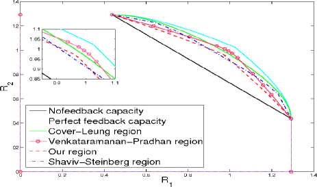
Figure 1: Achievable regions for the Gaussian MAC for $P/\sigma^{2}=5$ and $R_{\textnormal{fb}}=2$

Figure 1 compares the achievable region in (25), to the nofeedback capacity region, the perfect feedback capacity region [2], the Cover-Leung [3] and Venkataramanan-Pradhan [6] regions for perfect feedback, and to the Shaviv-Steinberg region with rate-limited feedback [9].

For the sake of simplicity we restrict to the case where only common feedback is present ($Y_{1}=Y_{2}=\emptyset,\sigma_{1}^{2},\sigma_{2}^{2}\to\infty$) which reduces to Wyner-Ziv coding [11] over the feedback links. In this case, we need to have $\sigma_{12}^{2}\geq\frac{\sigma^{2}+P}{2^{2R_{\textnormal{fb}}}-1}$ and we see that our scheme is strictly better in terms of sum-rate than the Shaviv-Steinberg scheme. In fact, based on extensive simulations, we conjecture that this is the case whenever $\frac{P}{\sigma^{2}}<2^{2R_{\textnormal{fb}}}-2$, which is equivalent to $\sigma_{12}^{2}<\sigma^{2}$.

References

• [1] N. T. Gaarder and J. K. Wolf, “The capacity region of a multiple-access channel can increase with feedback,” IEEE Trans. Inf. Theory, vol. IT-21, no. 1, pp. 100–102, 1975.
• [2] L. Ozarow, “The capacity of the white Gaussian multiple access channel with feedback,” IEEE Trans. Inf. Th., vol. 30, no. 4, pp. 623–629, 1984.
• [3] T. M. Cover and C. S. K. Leung, “An achievable rate region for the multiple-access channel with feedback,” IEEE Trans. Inf. Theory, vol. 27, pp. 292–298, 1981.
• [4] F. M. J. Willems, “The feedback capacity region of a class of discrete memoryless multiple-access channels,” IEEE Trans. Inf. Theory, vol. IT-28, no. 1, pp. 93–95, 1982.
• [5] S. I. Bross and A. Lapidoth, “An improved achievable region for the discrete memoryless two-user multiple-access channel with noiseless feedback,” IEEE Trans. Inf. Theory, vol. 51, no. 3, pp. 811–833, 2005.
• [6] R. Venkataramanan and S. S. Pradhan, “A new achievable rate region for the multiple-access channel with noiseless feedback”, IEEE Trans. Inf. Theory, vol. 57, no. 12, pp. 8038–8054, 2011.
• [7] A. B. Carleial, “Multiple-access channels with different generalized feedback signals,” IEEE Trans. Inf. Theory, vol. 28, pp. 841–850, 1982.
• [8] A. Lapidoth and M. Wigger, “On the AWGN MAC with imperfect feedback,” IEEE Trans. Inf. Theory, vol. 56, no. 11, pp. 5432–5476, 2010.
• [9] D. Shaviv and Y. Steinberg, “On the multiple-access channel with common rate-limited feedback,” IEEE Trans. Inf. Theory, vol. 59, no. 6, pp. 3780–3795, 2013.
• [10] C. Heegard and T. Berger, “Rate-distorsion when side-information may be absent,” IEEE Trans. Inf. Theory, vol. 31, no. 6, pp. 727–734, 1985.
• [11] A. D. Wyner and J. Ziv, “The rate-distortion function for source coding with side information at the decoder,” IEEE Trans. Inf. Theory, vol. 22, pp. 1–10, 1976.