Complex synchronization patterns in the human connectome network

Abstract

A major challenge in neuroscience is posed by the need for relating the emerging dynamical features of brain activity with the underlying modular structure of neural connections, hierarchically organized throughout several scales. The spontaneous emergence of coherence and synchronization across such scales is crucial to neural function, while its anomalies often relate to pathological conditions. Here we provide a numerical study of synchronization dynamics in the human connectome network. Our purpose is to provide a detailed characterization of the recently uncovered broad dynamic regime, interposed between order and disorder, which stems from the hierarchical modular organization of the human connectome. In this regime –similar in essence to a Griffiths phase– synchronization dynamics are trapped within metastable attractors of local coherence. Here we explore the role of noise, as an effective description of external perturbations, and discuss how its presence accounts for the ability of the system to escape intermittently from such attractors and explore complex dynamic repertoires of locally coherent states, in analogy with experimentally recorded patterns of cerebral activity.

1 Introduction

The current mapping of neural connectivity patterns relies on advanced neuro-imaging techniques, which have recently allowed for the reconstruction of structural human brain networks, establishing at an individual-based level which brain regions are mutually connected, as well as the strength of pairwise connections. The resulting “human connectome network” [1, 2] has been found to be structured in moduli or compartments –characterized by a much larger intra than inter connectivity– organized in a hierarchical fractal-like fashion across diverse scales [3, 4, 5, 6, 7, 8]. On the other hand, functional connections between different brain regions can be inferred e.g. from correlations in neural activity as detected in EEG or fMRI time series. Unveiling the relation between structural and functional networks is a current challenge in modern neuroscience. In this context, a few pioneering works found that the hierarchical-modular organization of structural brain networks has remarkable implications for neural dynamics [7, 9, 10, 11]. As opposed to the case of simpler network structures, neural activity propagates in hierarchical networks in a peculiar way. For example, models of neural activity propagation usually exhibit two familiar phases –percolating and non-percolating, respectively– but it has been recently found [12] that when such models operate on top of the “human connectome” structural network a novel intermediate regime, named a “Griffiths phase” [13, 14] emerges. This novel phase originates from the highly-diverse and relatively isolated structural moduli where dynamical activity may remain mostly localized for long time periods [12, 14].

Given that the correct brain functioning requires coherent neural activity at a wide range of scales [15, 16], the study of synchronization among neural populations is one of the central ideas in computational neuroscience [17, 18].

In a recent work [19], some of us scrutinized the special features of synchronization dynamics [20] using the canonical Kuramoto model for phase synchronization [21, 22, 23], in the actual human connectome (HC) network [1, 2, 24]. In analogy to what described above for activity propagation, we uncovered the existence of a novel intermediate phase for synchronization dynamics, stemming from the hierarchical modular organization of the HC. Furthermore, we found that the dynamics in such a region presented a plethora of complex and interesting dynamical features [19].

Our goal here is to describe in more detail the complex behavior within such an intermediate regime, both in individual moduli and at a global brain level. We measure the fluctuations of the global order parameter as a function of the overall coupling strength, and we show that there is a broad region (rather than a unique “critical” point) with huge variability and response. Finally, we assess the role of noise and perturbations in the robustness of the metastable stated arising in the intermediate regime, and we show that adding intrinsic fluctuations to the picture of synchronization dynamics in hierarchical modular networks accounts for the ability of the brain to explore different attractors, giving access to the varied functional configurations recorded in experiments [25, 26, 27].

2 Kuramoto model in the Human-Connectome network

The HC network we employ consists of a set of $N=998$ nodes, each of them representing a population of neurons producing self-sustained oscillations [28], connected pairwise through a precise pattern of symmetric weighted edges, altogether determining a connectivity matrix $\mathbf{W}$ [1, 2].

On top of such a HC network, we implement a noisy Kuramoto dynamics, defined by the set of differential equations [21, 22, 23]:

$${\dot{\theta}}_{i}(t)=\alpha\eta_{i}(t)+\omega_{i}+k\sum_{j=1}^{N}W_{ij}\sin\left[\theta_{j}(t)-\theta_{i}(t)\right],$$ (1)

where ${\theta}_{i}(t)$ is the phase at node $i$ at time $t$, the intrinsic frequencies $\omega_{i}$ –accounting for region heterogeneity– are extracted from some probability distribution function $g(w)$, $W_{ij}$ are the elements of the $N\times N$ weighted connectivity matrix $\mathbf{W}$, $k$ is an overall coupling parameter and $\eta_{i}(t)$ is a zero-mean delta-correlated Gaussian noise, tuned by the real-valued amplitude $\alpha$.

The Kuramoto complex order parameter is defined by $Z(t)=R(t)e^{i\psi(t)}=\langle e^{i\theta_{k}(t)}\rangle_{k}$, where $0\leq R\leq 1$ gauges the overall coherence and $\psi(t)$ is the average phase. It is common wisdom that for an (infinitely) large population of oscillators interacting in a fully connected network, the model exhibits a phase transition at some value of $k$, separating a coherent steady state ($R>0$) from an incoherent one ($R=0$, plus $1/\sqrt{N}$ finite-size corrections) [21, 22, 23]. On the other hand, in the absence of frequency heterogeneity the system always reaches a coherent state. Thus, frequency heterogeneity is responsible for frustrating synchronization if the coupling strength is weak. Similarly, in our recent work [19] we argued that the combined effect of frequency heterogeneity and network heterogeneity (in particular, a hierarchical modular structure) can lead to much richer and interesting ways of ordering frustration. Here we explore that phenomenology in much deeper detail, introducing external stochastic fluctuations (i.e. noise) as the mechanism accounting for the ability of the system to explore metastable configurations.

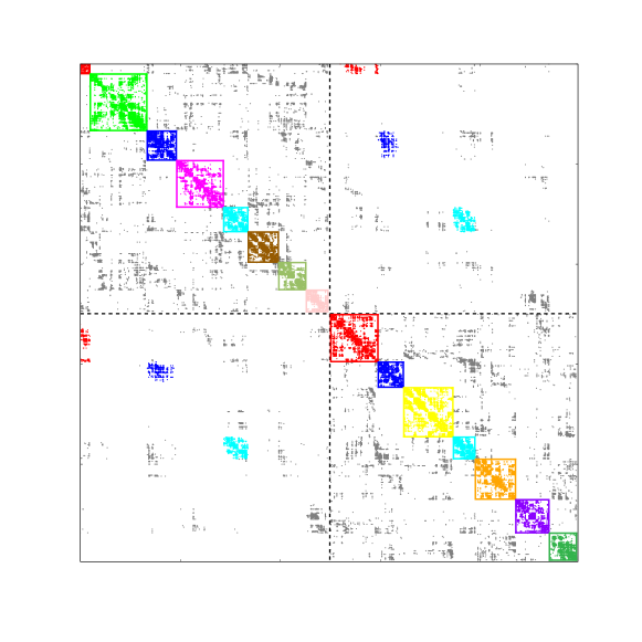
Figure 1: Adjacency matrix of the HC network with nodes ordered to emphasize its modular structure as highlighted by a community detection algorithm (see main text), showing also the partition into the $2$ hemispheres (dashed lines). $12$ moduli can be distinguished (each plotted with a different color); $4$ of them correspond to one of the two hemispheres, $5$ to the other, and only $3$ moduli overlap with both hemispheres (cyan, blue and red moduli). Inter-modular connections (grey) are limited to small subsets, acting as interfaces or connectors between moduli.

3 Results

We considered the HC network [1, 2] and employed standard community detection algorithms [29, 8] to identify the underlying modular structure. The optimal partition into communities –i.e. the one maximizing the modularity parameter [30]– turns out to correspond to a division in $12$ moduli [19]. At a higher hierarchical level, a separation into just $2$ moduli (roughly corresponding to the $2$ cerebral hemispheres) also provides a quite high modularity value. As illustrated in Fig. 1, $4$ (out of the $12$) moduli belong to one of the two hemispheres, $5$ to the other, while $3$ moduli (cyan, blue and red) overlap with both hemispheres. We label these two hierarchical levels as $l=2$ ($2$ large moduli) and $l=1$ ($12$ smaller moduli), respectively.

We have conducted computational analyses of the noisy Kuramoto model on top of the HC network and performed a number of new computational experiments complementing the analyses in our previous work [19].

Figure 2: (Main) Time-averaged value of the order parameter for the noisy Kuramoto dynamics running upon the Human Connectome network ($998$ nodes) with a Gaussian distribution of frequencies. Three different regimes emerge: an incoherent phase ($k<1.6$), a synchronous one ($k>3.3$), and an intermediate irregular one. In this last, much larger averaging times would be required to obtain reliable mean values and these would depend upon initial conditions, reflecting metastability. We have chosen not so large measuring times ($t=100$ for all values of $k$) to illustrate the variability in the intermediate region. (Inset) Time-series for $4$ different $k$ values, indicated by arrows in the x-axis (from left to right: $k=0.5,2.7,3.0$ and $4.0$).

As illustrated in Fig. 2, beside the aforementioned coherent and incoherent phases (usually encountered in synchronizing systems) there is an intermediate regime between them exhibiting a large variability. Individual trajectories are depicted in the inset, for different values of the coupling strength $k$; observe in particular the irregular oscillations obtained for intermediate values of $k$.

The reported values of $\langle R\rangle_{t}$ in the main plot of Fig. 2 correspond to the time-averaged value for a single realization in its steady state, considering up to a fixed maximum time $T$. The observed variability in the central region means either that (i) larger time windows would be required for the system to self-average or (ii) that ergodicity is broken and for each parameter value the realization ends up in a different type of (stable or metastable) steady state, depending on the initial condition. This last possibility implies that the system may remain trapped in some sort of metastable states, from which it can escape away only after very rare and large fluctuations.

These observations are robust against changes in the frequency distribution, connectivity matrix normalization, and other details, whereas the location and width of the intermediate phase are not universal. For example, Fig. 2 has been obtained for a Gaussian frequency distribution but similar curves are obtained for, usually employed, Lorentzian or uniform distributions.

As this robust intermediate regime is reminiscent of Griffiths phases in networks –posed in between order and disorder and emerging from rare-region effects [13, 14, 12]– it is natural to wonder how the structural network modularity affects synchronization dynamics in general. As a matter of fact, it is straightforward to convince oneself that any network consisting of perfectly isolated moduli, each of them synchronized at different intrinsic frequencies and phases, should exhibit oscillations of the collective order parameter, $R$, and these oscillations are preserved when the moduli are weakly interconnected [19]. Thus, in large networks without delays or other additional ingredients, time oscillations in the global coherence are the trademark of an underlying modular structure.

To illustrate the role played by internal network modularity on global synchronization, Fig. 3 portraits the trajectories of the parameter $Z(t)$ in the complex plane for different values of the control parameter $k$, measured at different hierarchical levels: two (out of the existing $12$) different small moduli (violet and orange curves), the two hemispheres (red and green), and the overall brain (blue). In the incoherent phase (panel a), the real and imaginary parts of $Z$ fluctuate around zero at all scales in the hierarchy. On the other hand, in the coherent phase (panel d), all nodes are synchronized, and trajectories are circles with radii close to unity at all hierarchical levels

A much richer behavior is found in the intermediate region: panel b (left) illustrates a situation in which one modulus (orange) is mostly coherent, while the other (violet) is not; however, hemispheres and global dynamics remain mostly unsynchronized (panel b (right)). In panel c (left), we have slightly increased the control parameter with respect to panel b, with a subsequent increase of the coherence for all hierarchical levels. Interestingly, as not all moduli exhibit the same state of coherence, chaotic-like oscillations of the order parameter are observed at the global scale.

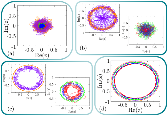
Figure 3: Phase portraits of the complex order parameter $Z(t)$, measured at different scales in the hierarchy for a Gaussian $g(w)$ (different realizations from those in Fig. 2): two of the existing moduli are plotted in violet and orange, respectively, the two hemispheres in red and green, and the global scale in blue. Panels (a)-(d) correspond to values of the control parameter $k=1,3,5$ and $8$, respectively (panels (b) and (c) have been split into two to enhance clarity). (a) In the non-ordered phase, the real and imaginary components of $Z$ fluctuate around zero, not exhibiting synchronization at any scale. (b) In the early region of the intermediate phase, a few moduli are coherent (as the one in orange) but most of them remain unsynchronized (violet), and the system does not present coherence for upper scales in the hierarchy. (c) Increasing $k$, more heterogeneity of synchronization among moduli is found, and the system exhibits complex trajectories for the intermediate (hemispheres) and global scale. (d) In the coherent phase, all moduli are synchronized, and trajectories are concentric circles.

We are interested in quantifying the observed variability of $R$ in the intermediate phase. To this end, we take a particular realization of frequencies (extracted from a Gaussian $g(w)$) and, starting from an initial –uniformly distributed– random configuration of individual phases, $\{\theta_{i}(t=0)\}_{i=1}^{N}$, we measure the temporal standard deviation of the global coherence parameter $R$ (after the transient) up to a maximum time $T=10^{4}$,

$$\sigma=\left(\langle\left(R-\langle R\rangle_{t}\right)^{2}\rangle_{t}\right)^{1/2}$$ (2)

as a function of the coupling strength $k$.

As ergodicity may be broken, different initial conditions may lead to different attractors of the dynamics, therefore we also average $\sigma$ over $100$ different independent realizations of the dynamical process. Results are illustrated in Fig. 4, in which we also have plotted the diagram of the order parameter obtained for this particular realization of $g(\omega)$ averaged over the $100$ realizations. Let us stress the following salient aspects: i) averaged time variabilities are small in the non-coherent ($k\lesssim 1$) as well as in the coherent ($k\gtrsim 5$) phases, whereas much larger variabilities are found in the intermediate region ($1\lesssim k\lesssim 5$); ii) the curve of time variabilities presents several peaks for the intermediate region, lying in the vicinity of values of the control parameter at which the system experiences a change in its level of coherence (see the corresponding jumps in the derivative of the order parameter); and finally, iii) error bars are also larger in the intermediate phase; this variability of time variabilities means that different initial conditions can lead to different types of time-series, suggesting a large degree of metastability in the intermediate regime.

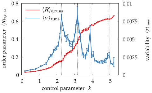
Figure 4: Time-averaged order parameter $R=\langle R(t)\rangle$ and standard deviation of time-series, averaged over realizations with different –uniformly distributed– initial conditions. Maximal variability is found in the intermediate phase, where the system is neither too unsynchronized nor too coherent. Several peaks in the variability can be distinguished (dashed lines), which appear at values of the control parameter $k$ for which the system experiments a fast increase in global synchronization. Statistical sampling of different realizations indicate that errorbars are larger in the intermediate region, suggesting the existence of several attractors depending on the initial conditions. We have averaged $100$ different realizations, each one integrated for $10^{4}$ time steps.

3.1 Metastability in HMNs

Our previous results vividly illustrate the existence of an intermediate region in which the HC exhibits maximal dynamical variability at the global scale, suggesting metastable behavior. In order to explore more directly whether metastable states exist, we now assess if the dynamics may present different attractors and, for some values of the control parameter $k$ and noise amplitudes, if the system may switch between different global attractors with different levels of coherence.

Fig. 5 (a) shows a time series of the global parameter, for a fixed realization of internal frequencies and initial phases. It clearly illustrates how the HC spontaneously switches between two different attractors. These type of events, however, are not easy to observe in the HC network. Due to the coarse-grained nature of the HC mapping, different attractors may actually have comparable average values of the coherence $R$, which makes their discrimination especially difficult at the global scale.

Instead, such events are easier to spot in synthetic hierarchical modular networks (HMN), such as proposed to model brain networks in an efficient way (see [12] and references therein). In such hierarchical networks, the effects of modularity and hierarchy are much enhanced, as they develop across a larger number of hierarchical levels than the one allowed by current imaging techniques for empirically obtained connectomes.

All the previously reported phenomenology is still present in such HMNs (see [19]); in particular, the phase diagram of the synchronization order parameter exhibits a phase transition with an intermediate region, where variability is much enhanced [19]. Fig. 5 (b) illustrates the bi-stable nature of the global parameter in the intermediate phase for a HMN, in which metastability can be very well appreciated. This switching behavior closely resembles “up and down” states, which are well known to appear in certain phases of sleep or under anaesthesia (see [32] and refs. therein).

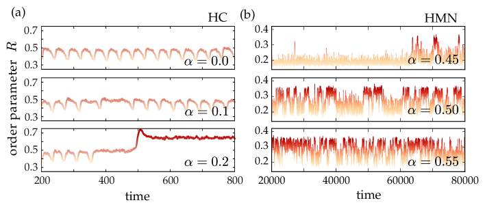
Figure 5: Time series exhibit metastability of the global synchronization in the Human Connectome and in HMNs, in the intermediate region. (a) Times series of the noisy Kuramoto dynamics in the HC with Gaussian $g(w)$ in the intermediate region: for low noise amplitudes ($\alpha=0$ and $0.1$), the system stays stable in the same attractor. But, for sufficiently large values, such as $\alpha=0.2$, the system is able to “jump” to another more coherent attractor, where it settles. (b) In HMNs (size $N=1024$, $9$ hierarchical levels), we observe the same phenomenology, but much enhanced: when noise is very low ($\alpha\leq 0.45$), the system tends to remain stable in a certain attractor (with a few exceptions after very large waiting times). Choosing a higher $\alpha$ ($\alpha\geq 0.5$), the system exhibits bi-stable behavior, switching intermittently between two different attractors. For large enough $\alpha$ ($\alpha\geq 0.55$), the dynamics becomes too erratic to appreciate metastability. Here, frequencies were extracted from a Lorentz distribution.

We hypothesize that hierarchical modular networks in general (and the HC in particular) enable the possibility of a large repertoire of attractors, with different degrees of coherence and stability. Such metastability can be made evident and quantified by performing the following type of numerical test. Starting from a fixed random initial condition and considering a vanishing noise amplitude (i.e. $\alpha=0$), the system might deterministically fall into a number of different attractors, each of them with an associated value of the global coherence depending on the initial conditions, the network structure, and the choice of natural frequencies. Once this attractor A is reached, the system is perturbed by switching on a non-vanishing noise amplitude ($\alpha>0$) during a finite time window. The system may remain stable in the same attractor A if the noise is weak enough ($\alpha\ll 1$). However, if larger values of the noise amplitude are chosen, the system may jump into another close, more stable, attractor. If the noise amplitude is very large ($\alpha\gg 1$), the system can in principle jump to any attractor, but, very likely, will also escape from it, wandering around a large fraction of the configuration space. After the perturbation time-window is over, we let the system relax once again, and check if the new resulting steady steady state B has changed with respect to A. In that case, we can conclude that the systems was in a metastable state A before the perturbation, and has reached another state B after it – potentially a metastable state itself.

We have carried out this type of test using an artificial HMN (see Fig. 6) for a specific value of the control parameter, $k$, belonging in the intermediate region. Natural frequencies are sampled from the a Lorentzian distribution $g(\omega)$ (as above, our main results are not sensible to this choice). Starting from a random initial configuration of phases, we integrate Eq. 1 up to time $500$ with $\alpha=0$. After this, we introduce the external perturbation by switching the noise coefficient $\alpha$ to a certain non-zero value during a time window of duration $100$. Finally we revert to $\alpha=0$ and continue the integration up to time $t=1000$. The last steady state value is averaged over $10^{4}$ realizations of initial conditions, networks, and intrinsic frequencies.

As illustrated in Fig. 6, for low as well as for high values of the noise amplitude, the system has the same average order parameter close to $\langle R\rangle_{t,\mathrm{runs}}\simeq 0.2$, as could have been anticipated. However, a resonant peak emerges for intermediate values of the noise, where the system switches to states with different levels of coherence. This plot explicitly illustrates the existence of metastability and noise-induced jumps between attractors. As noise is enhanced, progressively more stable states are found, but above some noise threshold, the system does not remain trapped in a single attractor but jumps among many, resulting in a progressive decrease of the overall coherence.

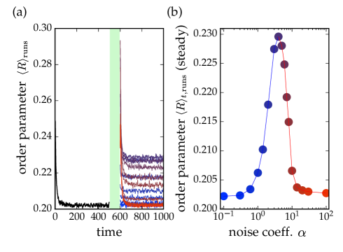
Figure 6: Perturbations can lead the system to more coherent attractors in the intermediate non-coherent phase. (a) Order parameter $R$ averaged in time over $10^{4}$ realizations. A noise pulse of amplitude $\alpha$ is applied during the green interval. This same protocol is repeated for different values of $\alpha$. (b) Average order parameter in the final steady state (after the noise pulse) as a function of $\alpha$. For intermediate values of $\alpha$, a resonant peak emerges for $1<\alpha<10$, illustrating that the system can jump to a close, more coherent on-average attractor. Simulations are run on HMN networks of size $N=1024$, with $9$ hierarchical levels.

4 Discussion

It is well established that in the absence of frequency dispersion, the Kuramoto dynamics leads to a perfectly coherent state, which is progressively achieved in time by following a bottom-up ordering dynamics in which increasingly larger communities become synchronized [33].

If a hierarchical modular networks is loosely connected, this type of “matryovska-doll” synchronization process is constrained at all levels by structural bottlenecks, bringing about anomalously-slow synchronization dynamics as recently reported [19].

In the presence of intrinsic frequency dispersion the above slow ordering process is further frustrated [19]. For small values of $k$ the system may remain trapped into metastable states in which the loose connectivity between some moduli does not allow them to overcome intrinsic-frequency differences and achieve coherence. While persistence in metastable states may extend indefinitely, experimental evidence suggests that the brain is able to switch between a rich repertoire of attractors [25, 26, 27]. We have shown that a simple description of neural coherence dynamics based on the noisy Kuramoto model may suffice to reproduce a very rich phenomenology, in hierarchical modular networks and in particular in the human connectome. The introduction of small fluctuations (exemplifying external perturbations, stimuli, or intrinsic stochasticity) allow the system to escape from metastable states and sample the configuration space, proving a paradigmatic modeling tool for the attractor surfing behavior suggested by experiments. Additional ingredients, such as explicit phase frustration [31] or time delays [28, 34], should only add complexity to the structural frustration effect reported here, providing a finer description of brain activity.

References

- [1] Hagmann, P., Cammoun, L., Gigandet, X., Meuli, R., Honey, C.J., Wedeen, V.J., Sporns, O.: Mapping the structural core of human cerebral cortex. PLoS Biol. 6(7), e159 (2008)
- [2] Honey, C.J., Sporns, O., Cammoun, L., Gigandet, X., Thiran, J.P., Meuli, R., Hagmann, P.: Predicting human resting-state functional connectivity from structural connectivity. Proc. Natl. Acad. Sci. 106(6), 2035–2040 (2009)
- [3] Bullmore, E., Sporns, O.: Complex brain networks: graph theoretical analysis of structural and functional systems. Nat. Rev. Neurosci. 10, 186–98 (2009)
- [4] Sporns, O.: Networks of the Brain. MIT Press, Cambridge (2010)
- [5] Kaiser, M.: A tutorial in connectome analysis: topological and spatial features of brain networks. NeuroImage 57(3), 892–907 (2011)
- [6] Meunier, D., Lambiotte, R., Bullmore, E.: Modular and hierarchically modular organization of brain networks. Front. Neurosci. 4, 200 (2010)
- [7] Zhou, C., Zemanova, L., Zamora-López, G., Hilgetag, C.C., Kurths, J.: Hierarchical Organization Unveiled by Functional Connectivity in Complex Brain Networks. Phys. Rev. Lett. 97(23) (2006)
- [8] Ivković, M., Amy, K., Ashish, R.: Statistics of Weighted Brain Networks Reveal Hierarchical Organization and Gaussian Degree Distribution. PLoS ONE 7(6), e35029 (2012)
- [9] Zhou, C., Zemanova, L., Zamora-López, G., Hilgetag, C.C., Kurths, J.: Structure–function relationship in complex brain networks expressed by hierarchical synchronization. New J. Phys. 9(6), 178–178 (2007)
- [10] Kaiser, M., Goerner, M., Hilgetag, C.: Criticality of spreading dynamics in hierarchical cluster networks without inhibition. New J. Phys. 9, 110 (2007)
- [11] M. Kaiser, C.H.: Optimal Hierarchical Modular Topologies for Producing Limited Sustained Activation of Neural Networks. Front. in Neuroinform. 4, 8 (2010)
- [12] Moretti, P., Muñoz, M.A.: Griffiths phases and the stretching of criticality in brain networks. Nat. Commun. 4, 2521 (2013)
- [13] Vojta, T.: Rare region effects at classical, quantum and nonequilibrium phase transitions. J. Phys. A 39(22), R143–R205 (2006)
- [14] Muñoz, M.A., Juhász, R., Castellano, C., Ódor, G.: Griffiths Phases on Complex Networks. Phys. Rev. Lett. 105, 128701 (Sep 2010)
- [15] Steinmetz, P.N., Roy, A., Fitzgerald, P.J., Hsiao, S.S., Johnson, K.O., Niebur, E.: Attention modulates synchronized neuronal firing in primate somatosensory cortex. Nature 404(6774), 187–190 (2000)
- [16] Kandel, E.R., Schwartz, J.H., Jessell, T.M.: Principles of Neural Science. McGraw-Hill, New York (2000)
- [17] Buzsáki, G.: Rhythms of the Brain. Oxford University Press, NY (2006)
- [18] Breakspear, M., Stam, C.J.: Dynamics of a neural system with a multiscale architecture. Phil. Trans. R. Soc. Lond. B 360(1457), 1051–1074 (2005)
- [19] Villegas, P., Moretti, P., Muñoz, M.A.: Frustrated hierarchical synchronization and emergent complexity in the human connectome network. Sci. Rep. 4, 5990 (2014)
- [20] Rosenblum, M.G., Pikovsky, A., Kurths, J.: Synchronization – A universal concept in nonlinear sciences. Cambridge University Press, Cambridge (2001)
- [21] Kuramoto, Y.: Self-entrainment of a population of coupled nonlinear oscillators. Lect. Not. in Phys. 39, 420–422 (1975)
- [22] Strogatz, S.H.: From kuramoto to crawford: exploring the onset of synchronization in populations of coupled oscillators. Physica D: 143(1), 1–20 (2000)
- [23] Acebrón, J.A., Bonilla, L.L., Pérez-Vicente, C.J., Ritort, F., Spigler, R.: The Kuramoto model: A simple paradigm for synchronization phenomena. Rev. Mod. Phys. 77, 137–185 (2005)
- [24] Arenas, A., Díaz-Guilera, A., Kurths, J., Y. Moreno, Y., Zhou, C.: Synchronization in complex networks. Phys. Rep. 469(3), 93–153 (2008)
- [25] Chialvo, D.R.: Emergent complex neural dynamics. Nature Phys. 6, 744–750 (2010)
- [26] Deco, G., Jirsa, V.K.: Ongoing Cortical Activity at Rest: Criticality, Multistability, and Ghost Attractors. Jour. of Neurosci. 32(10), 3366–3375 (2012)
- [27] Haimovici, A., Tagliazucchi, E., Balenzuela, P., Chialvo, D.R.: Brain Organization into Resting State Networks Emerges at Criticality on a Model of the Human Connectome. Phys. Rev. Lett. 110, 178101 (2013)
- [28] Cabral, J., Hugues, E., Sporns, O., Deco, G.: Role of local network oscillations in resting-state functional connectivity. NeuroImage 57(1), 130–139 (2011)
- [29] Duch, J., Arenas, A.: Community detection in complex networks using extremal optimization. Phys. Rev. E 72, 027104 (2005)
- [30] Newman, M.: The Structure and Function of Complex Networks. SIAM Review 45(2), 167–256 (2003)
- [31] Shanahan, M.: Metastable chimera states in community-structured oscillator networks. Chaos 20(1), 013108 (2010)
- [32] Eckmann, J.P., Feinerman, O., Gruendlinger, L., Moses, E., Soriano, J., Tlusty, T.: The physics of living neural networks. Phys. Rep. 449(1-3), 54–76 (2007)
- [33] Arenas, A., Díaz-Guilera, A., Pérez-Vicente, C.: Synchronization reveals topological scales in complex networks. Phys. Rev. Lett. 96, 114102 (2006)
- [34] Wildie, M., Shanahan, M.: Metastability and chimera states in modular delay and pulse-coupled oscillator networks. Chaos 22(4), 043131+ (2012)