Study of vorticity in an exact rotating hydro model

Abstract

We study a semianalytic exact solution of the fluid dynamical model of heavy ion reactions, and evaluate some observable signs of the rotation.

1 Introduction

In peripheral heavy ion collisions the system has angular momentum.[1] It has been shown in hydrodynamical computations that the angular momentum leads to a large shear and vorticity [2]. Furthermore when the Quark-Gluon Plasma (QGP) is formed with low viscosity [3], interesting new phenomena may occur like rotation [4], or turbulence, which shows up in form of a starting Kelvin-Helmholtz instability (KHI) [5, 6]. The deceleration of interpenetrating nuclei was observed and analyzed early in Ref. [7]. This leads to a rapid initial equilibration and to the development of a compact initial system. In peripheral collision this leads to considerable initial shear and vorticity, as well as to an almost complete conservation of the initial pre-collision angular momentum for the participants.

Based on Refs. [2, 5] we can extract some basic parameters of the rotation obtained with numerical fluid dynamical model PICR. These parameters are extracted from model calculation of a Pb+Pb collision at $\sqrt{s_{NN}}=2.76$ TeV/nucl. and impact parameter $b=0.7b_{max}$, with high resolution and thus small numerical viscosity. Thus, in this collision the KHI occurs and enhances rotation at intermediate times, because the turbulent rotation gains energy from the original shear flow. The turbulent rotations leads to a rotation profile where the rotation of the external regions lags behind the rotation of the internal zones. This is a typical growth of the KHI.

The time dependence of some characteristic parameters of the fluid dynamical calculation [5] were analysed in Ref. [8]. It was observed that R, the average transverse radius, Y, the longitudinal (rotation axis directed) length of the participant system, $\theta$, the polar angle of the rotation of the interior region of the system, are increasing with time. $\dot{R}$ and $\dot{Y}$ the speeds of expansion in transverse and axis directions are also increasing with time, while $\omega$ the angular velocity of the internal region of the matter during the collision is decreasing.

The initial angular momentum of the system is large, $L_{y}=-1.05\times 10^{4}\hbar$. As this is arising from the $z$ directed beam velocity, initially at the vertical, $x$, edges the velocity difference is large, while horizontally the rotation starts up delayed, because this is not a solid body rotation. Here we considered the rotation measure versus the horizontal, $z$ axis which starts up slower and reaches a maximum around 5 fm/c after the start of the fluid dynamical evolution, i.e. around 8 fm/c after the initial touch of the nuclear surfaces.

Exact models, see e.g. Ref. [9], provide good insight into physical phenomena. We want to use the above mentioned fluid dynamical calculations to test a new family of exact rotation solutions of fireball hydrodynamics [2, 10]. This model offers a few possible variations, here we chose the version 1A to test. We use the axis labeling of Refs. [2, 10], so that the the axis of the rotation is $y$ while the transverse plane of the rotation is the $[x,z]$ plane. Thus the values extracted from the results of the fluid dynamical model [5], should take this into account. The initial radius parameter, $R$, corresponds to the $x$ axis in hydro, and we assume an $x,z$ symmetry in the exact model, The rotation axis is the $y$ axis in hydro. The exact model assumes cylindrical symmetry, so it cannot describe the beam directed elongation of the system, but this is arising from the initial beam momentum, and we intend to describe the rotation of the interior part of the reaction plane and the rotation there.

For simplicity we also assume that the Equation of State (EoS) is

$$\epsilon=\kappa p\ \ \ {\rm and}\ \ \ p=nT\ ,$$ (1)

with a constant $\kappa$.

2 From the Euler Equation to Scaling

Now we calculate the equation of motion, (15) in Ref.[10], and its solution

$$n\,m\,(\partial_{t}+\mbox{\boldmath$v$}\cdot\nabla)\mbox{\boldmath$v$}=-\nabla p$$ (2)

For the variables of this equation we have:

$$T = T_{0}\left(\frac{V_{0}}{V}\right)^{1/\kappa}\mathcal{T}(s)\ ,$$

$$n = n_{0}\frac{V_{0}}{V}\nu(s),$$

$$\nu(s) = \frac{1}{\mathcal{T}(s)}e^{-\frac{1}{2}\int_{0}^{s}\frac{du}{\mathcal{T}(u)}},$$ (3)

and in addition in Ref. [10] it is assumed that the temperature and the density have time independent distributions with respect to a scaling variable:

$$s=r_{x}^{2}/R^{2}+r_{y}^{2}/Y^{2}+r_{z}^{2}/R^{2}\ .$$

If we asume cylindrical symmetry and use the coresponding cylindrical coordinates instead of $(x,y,z)$, we can use the coordinates of length dimension, $(r_{\rho},r_{\varphi},r_{y})$, so that

$$r_{\rho}=\rho,\ \ r_{\varphi}=r_{\rho}\varphi,\ \ r_{y}=y\ .$$

These are the ”out, side, long” directions. The characteristic values of these coordinates are then $(R,S,Y)$. Then the scaling variables are introduced as

$$s_{\rho}=r_{\rho}^{2}/R^{2},\ \ s_{\varphi}=r_{\varphi}^{2}/S^{2}\ \ s_{y}=r_{y}^{2}/Y^{2}\ ,$$

where $S$ is the roll-length on the outside circumference, starting from $\varphi_{0}=0$ and $S_{0}=0$ at $t_{0}$,   $S=R\varphi$ and $\dot{\varphi}~{}=~{}\omega$ and this displacement is orthogonal to the longitudinal and transverse displacements. The internal roll-length $r_{\varphi}=\varphi\,r_{\rho}$, the corresponding velocity is $v_{\varphi}=\omega\,r_{\rho}$, and so $v_{\varphi}^{2}=\omega^{2}\,r_{\rho}^{2}$. On the other hand from the scaling of $r_{\rho}$, it follows that $r_{\rho}^{2}=R^{2}\,s_{\rho}$.

In case of these scaling variables the distributions of density and temperature, $n(s)$ and $T(t,s)$ should not depend on $s_{\varphi}$ or $r_{\varphi}$, just on the radius and the longitudinal coordinates. Therefore just as in Ref. [8] we introduce another scaling variable:

$$s\equiv s_{\rho}+s_{y}\ .$$

Our reference frame is then spanned by the directions $(r_{\rho},r_{\varphi},r_{y})$. In this case due to the cylindrical symmetry the derivatives, $\partial s/\partial r_{\varphi}$ vanish. In this coordinate system the volume is $V=\pi R^{2}Y$.

Now following Ref. [8], for the right hand side of Eq. (2): For the r.h.s. of this equation we have:

$$-\nabla p = -\nabla nT$$ (4)

$$= -n_{0}\frac{V_{0}}{V}T_{0}\left(\frac{V_{0}}{V}\right)^{1/\kappa}\nabla e^{-\frac{1}{2}\int_{0}^{s}\frac{du}{\mathcal{T}(u)}}$$

$$= -n_{0}\frac{V_{0}}{V}T_{0}\left(\frac{V_{0}}{V}\right)^{1/\kappa}e^{-\frac{1}{2}\int_{0}^{s}\frac{du}{\mathcal{T}(u)}}(-\frac{1}{2})\frac{1}{\mathcal{T}(s)}\nabla s$$

$$= nmQ/V^{\gamma}\left(\frac{r_{\rho}}{R^{2}}\mbox{\boldmath$e$}_{\rho}{+}\frac{r_{z}}{Y^{2}}\mbox{\boldmath$e$}_{z}\right)$$

where $\gamma=1/\kappa$ and $Q\equiv\frac{T_{0}V_{0}^{\gamma}}{m}$.

Using the $\rho,\varphi,y$ coordinates, the rotation would show up as an independent orthogonal term. However, (as discussed in the Appendix) the closed system has no external torque, and the internal force from the gradient of the pressure is radial, which does not contribute to tangential acceleration. The change of the angular velocity arises from the angular momentum conservation in the closed system as a constraint, so we do not have to derive additional dynamical equations to describe the evolution of the rotation.

Now for the left hand side of Eq. (2), the velocity field scales as

$$\mbox{\boldmath$v$}=v_{\rho}\mbox{\boldmath$e$}_{\rho}{-}v_{\varphi}\mbox{\boldmath$e$}_{\varphi}{+}v_{z}\mbox{\boldmath$e$}_{z}=\frac{\dot{R}}{R}r_{\rho}\mbox{\boldmath$e$}_{\rho}{-}\omega r_{\rho}\mbox{\boldmath$e$}_{\varphi}{+}\frac{\dot{Y}}{Y}r_{y}\mbox{\boldmath$e$}_{y}\ .$$ (5)

We first calculate the time derivatives for the components. (See e.g. [11]):

$$\partial_{t}v_{\rho} = \left[\left(\frac{\ddot{R}}{R}{-}\frac{\dot{R}^{2}}{R^{2}}\right)-\omega^{2}\right]r_{\rho},$$

$$\partial_{t}v_{\varphi} = -\omega\frac{\dot{R}}{R}r_{\rho},\ \ \ \partial_{t}v_{z}=\left[\frac{\ddot{Y}}{Y}{-}\frac{\dot{Y}^{2}}{Y^{2}}\right]r_{y}.$$ (6)

The other term of the comoving derivative includes

$$\mbox{\boldmath$v$}\cdot\nabla=v_{\rho}\frac{\partial}{\partial r_{\rho}}+v_{\varphi}\frac{\partial}{\partial r_{\varphi}}+v_{y}\frac{\partial}{\partial r_{y}}$$ (7)

and this term gives:

$$(\mbox{\boldmath$v$}\cdot\nabla)\mbox{\boldmath$v$}=\frac{\dot{R}^{2}}{R^{2}}r_{\rho}\mbox{\boldmath$e$}_{\rho}+\omega\frac{\dot{R}}{R}r_{\rho}\mbox{\boldmath$e$}_{\varphi}+\frac{\dot{Y}^{2}}{Y^{2}}r_{y}\mbox{\boldmath$e$}_{y}$$ (8)

By adding Eq. (6) and (8) we get:

$$mn(\partial_{t}{+}\mbox{\boldmath$v$}\cdot\nabla)v_{\rho} = mn\left[\left(\ddot{R}/R\right)-\omega^{2}\right]r_{\rho}\ ,$$

$$mn(\partial_{t}{+}\mbox{\boldmath$v$}\cdot\nabla)v_{y} = mn\left(\ddot{Y}/Y\right)r_{y}\ .$$ (9)

As a consequence the equality of the right hand side and left hand side of the Euler equation (2) leads to the ordinary differential equations. Multiplying the two non-vanishing equations with $R^{2}$ and $Y^{2}$ respectively yields:

$$R\ddot{R}-W/R^{2} = Y\ddot{Y}=\frac{Q}{(\pi R^{2}Y)^{\gamma}}\ ,$$ (10)

where $W~{}\equiv~{}\omega_{0}^{2}~{}R_{0}^{4}$. From the angular momentum conservation $\omega=\omega_{0}R_{0}^{2}/R^{2}$, and the rotational term, $R^{2}\omega^{2}$ that appears in the equation, takes the form $W/R^{2}$.

Due to the EoS the pressure is proportional to the baryon density $n$, just as the r.h.s. of the Euler equation, therefore the equation of motion does not depend on $n$ or $n_{0}$.

3 Conservation Laws

Following Ref. [8], we want to calculate the total energy of the whole system, then we should integrate it for the whole volume, $V$. Thus, not only the scaling of $\mbox{\boldmath$v$}=(v_{\rho},v_{\varphi},v_{z})$ but also the particle density distribution, $n(s)$ will be considered.

At the surface the rotational energy is $\mathcal{E}_{Side}\equiv\frac{1}{2}m\dot{S}^{2}=\frac{1}{2}mR^{2}\omega^{2}$, and if we express $\omega$ via $\omega_{0}$ by the relation $\omega=\omega_{0}R_{0}^{2}/R^{2}$, then $\mathcal{E}_{Side}=W/R^{2}$, as before. The expansion energy at the surface is $\mathcal{E}_{Out}\equiv\frac{1}{2}m\dot{R}^{2}$, and for the longitudinal direction we have, $\mathcal{E}_{Long}\equiv\frac{1}{2}m\dot{Y}^{2}$.

We can calculate the radial and longitudinal expansion velocities and the corresponding kinetic energies, and also the kinetic energy of the rotation. In the evaluation of the internal and kinetic energies, the radial and longitudinal density profiles of the system are taken into account.

Let us assume that the temperature profile is flat, and thus that the density profiles are Gaussian and separable. Further if we assume that the system size is finite, then the scaling variables, $s_{\rho}$ and $s_{Y}$, may extend from 0 to 1. In this case at the external boundary we have to apply the necessary boundary conditions so that the solution of the Euler equation (2) remains valid. With this approximation we calculated the different integrated energies (and shown in Appendices 8-11).

Summing up the kinetic energies yields

$$E_{kin}=\frac{1}{2}mN_{B}\left(\alpha^{2}\dot{R}^{2}+\alpha^{2}R^{2}\omega^{2}+\beta^{2}\dot{Y}^{2}\right)\ ,$$ (11)

where in case of finite extent of the system
$\alpha^{2}\!\equiv\!4\sqrt{2}\,C_{n}I_{B}({\small\frac{1}{2}}s_{yM})I_{C}({\small\frac{1}{2}}s_{\rho M})\,{\rm and}\,$
$\beta^{2}\!\equiv\!4\sqrt{2}\,C_{n}I_{A}({\small\frac{1}{2}}s_{\rho M})I_{D}({\small\frac{1}{2}}s_{yM})$ where
$C_{n}=1\left/\left[2\sqrt{2}\,I_{A}(s_{\rho M}/2)\,I_{B}(s_{yM}/2)\right]\right.$, see Ref. [12] (in terms of the integrals evaluated in Appendices 8-11 ).

Here with $(s_{\rho M}=(s_{yM}=1$, $\alpha^{2}$ and $\beta^{2}$ are clearly time independent, because they depend on the scaling variable only, and we get the values $\alpha^{2}=0.4585$ and $\beta^{2}=0.2911$.

Alternatively one can assume that the system size is infinite so that the scaling variables range from 0 to $\infty$. In this case the Radius, and Length parameters, $R$ and $Y$, are considered as the width of the Gaussian scaling distribution. Thus the parameters will be

$$I_{A}=I_{B}=1,\ I_{C}=2I_{D}=\sqrt{\pi}$$ (12)

and consequently $\alpha^{2}=2.0$ and $\beta^{2}=1.0$. In the present case we follow this configuration.

If we divide this result by the conserved baryon charge, $N_{B}$, we will get

$$\frac{E_{kin}}{N_{B}}=\frac{1}{2}m\left[\alpha^{2}\left(\dot{R}^{2}{+}R^{2}\omega^{2}\right)+\beta^{2}\,\dot{Y}^{2}\right]\ ,$$ (13)

Based on the EoS, $\epsilon=\kappa p=\kappa nT$, we can calculate the compression energy based on the density profiles of $n(s)$ and $\epsilon(s)=\kappa\,n(s)T(s)$.

Let us make the same simplifying assumptions on the density profiles as we did earlier. Now we will have the same density profile, normalized to $N_{B}$, for the volume integrated internal energy and the net baryon charge:

$$E_{int} = \kappa\int pdV=\kappa\int nTdV$$ (14)

$$= \kappa N_{B}T_{0}(V_{0}/V)^{\gamma}\,C_{n}\,\frac{1}{V}\ \pi R^{2}\!\!\int_{0}^{1}Y\!\!\int_{0}^{1}\!\!\!\nu(s)\ ds_{\rho}\,\frac{ds_{z}}{\sqrt{s_{z}}}$$

$$= \kappa N_{B}T_{0}(V_{0}/V)^{\gamma}\ =\ \kappa mQ\frac{1}{(\pi R^{2}Y)^{\gamma}}\ ,$$

where $C_{n}$ is the normalization constant.

4 Reduction to a Single Differential Equation

Following the method of Ref. [13] , we study the following combination of variables:

$${\cal F} = {\small\frac{1}{2}}\partial_{t}^{2}\left(\alpha^{2}R^{2}+\beta^{2}Y^{2}\right)$$ (15)

$$= \partial_{t}\left(\alpha^{2}R\dot{R}+\beta^{2}Y\dot{Y}\right)$$

$$= \alpha^{2}\dot{R}^{2}+\beta^{2}\dot{Y}^{2}+\alpha^{2}R\ddot{R}+\beta^{2}Y\ddot{Y},$$

where we used the notation $\partial_{t}=\frac{\partial}{\partial t}\ \ {\rm and}\ \ \partial_{t}^{2}=\frac{\partial^{2}}{\partial t^{2}}.$ We can replace the last two terms, $\alpha^{2}R\ddot{R},\ \beta^{2}Y\ddot{Y}$, by using Eqs. (10), i.e. we use the Euler Eq. (2). Then we obtain:

$${\cal F}=\alpha^{2}\dot{R}^{2}+\beta^{2}\dot{Y}^{2}+\alpha^{2}\frac{W}{R^{2}}+(\alpha^{2}{+}\beta^{2})\frac{Q}{(\pi R^{2}Y)^{\gamma}},$$ (16)

At the same time from the energy conservation, $E_{tot}=E_{kin}+E_{int}$, we get that

$$\frac{E_{tot}}{N_{B}\,m}=\frac{1}{2}\left[\alpha^{2}\dot{R}^{2}{+}\beta^{2}\dot{Y}^{2}{+}\alpha^{2}\frac{W}{R^{2}}{+}\frac{2\kappa Q}{(\pi R^{2}Y)^{\gamma}}\right],$$ (17)

where we used the EoS and the parameter $\kappa$ now appears in the expression of the energy. If our EoS is such that

$$\kappa=\frac{1}{2}(\alpha^{2}{+}\beta^{2})=\frac{3}{2},$$ (18)

then ${\cal F}=2E_{tot}/(N_{B}\,m)=$ const., and in the same type of calculation as in Ref. [13], we can introduce

$$U^{2}(t)\equiv\alpha^{2}R^{2}(t)+\beta^{2}Y^{2}(t),$$ (19)

which satisfies

$$\partial_{t}^{2}\left(\alpha^{2}R^{2}+\beta^{2}Y^{2}\right)=\partial_{t}^{2}U^{2}(t)=2{\cal F}\ .$$ (20)

Thus, the solution of Eq. (20), we can be parameterized as:

$$U^{2}(t)=A(t-t_{0})^{2}+B(t-t_{0})+C\ ,$$ (21)

where

$$A = \alpha^{2}\dot{R}_{0}^{2}+\beta^{2}\dot{Y}_{0}^{2}+\alpha^{2}W/R_{0}^{2}+(\alpha^{2}{+}\beta^{2})\frac{T_{0}}{m}$$

$$B = 2\alpha^{2}R_{0}\dot{R}_{0}+2\beta^{2}Y_{0}\dot{Y}_{0}\phantom{\frac{T_{0}}{m}}$$

$$C = \alpha^{2}R_{0}^{2}+\beta^{2}Y_{0}^{2}\phantom{\frac{T_{0}}{m}}\ .$$ (22)

Due to the difficulties described in Appendix 12, we cannot use the method described in [13]. Instead let us take one of the Euler equations from Eq. (10),

$$\ddot{Y}=\frac{Q}{Y(\pi R^{2}Y)^{\gamma}}\ ,$$ (23)

and express $R^{2}$ in terms of $U^{2}(t)$ which is known based on the energy conservation:

$$R^{2}(t)=(U^{2}(t)-\beta^{2}Y^{2})/\alpha^{2}\ ,$$ (24)

and this will lead to the second order differential equation for $Y(t)$:

$$\ddot{Y}=\frac{\alpha^{2\gamma}\,Q}{Y\left[\pi Y(U^{2}(t){-}\beta^{2}Y^{2})\right]^{\gamma}}=f(Y,t)\ ,$$ (25)

which can be solved
Then $R(t)$ and $\dot{R}(t)$ are given by Eqs. (24) and (16) respectively.

${}^{|}_{|}$ $t$	$Y$	$\dot{Y}$	$R$	$\dot{R}$	$\omega$
(fm/c)	(fm)	(c)	(fm)	(c)	(c/fm)
0.0	4.000	0.400	2.500	0.250	0.150
1.0	4.440	0.469	2.859	0.704	0.115
2.0	4.922	0.490	3.405	0.834	0.081
3.0	5.415	0.495	4.079	0.877	0.056
4.0	5.912	0.497	4.833	0.894	0.040
5.0	6.409	0.497	5.636	0.902	0.030
6.0	6.906	0.498	6.469	0.906	0.022
7.0	7.404	0.498	7.322	0.909	0.017
8.0	7.901	0.498	8.190	0.911	0.014

Table 1: Time dependence of characteristic parameters of the exact fluid dynamical model [8]. R is the transverse radius, Y is the (rotation axis directed) length of the system, $\dot{R},\ \dot{Y}$ are the speed of expansion in transverse and axis directions, and $\omega$ is the angular velocity of the matter.

The derivatives, $\dot{R}(t_{0})$ and $\dot{Y}(t_{0})$ in this exact model do not equal the ones obtained from the fluid dynamical model, because in the more realistic fluid dynamical model the density and velocity profiles do not agree with the exact model’s assumptions. Also initially in the realistic fluid dynamical model the angular momentum increases in the region due to the developing turbulence, while in the exact model the angular velocity is monotonously decreasing due to the scaling expansion.

Figure 1: (Color online) The time dependence of the kinetic energy of the expansion, $E_{kin}$, the internal energy, $E_{int}$, the rotational energy, $E_{rot}$, and the total energy, $E_{tot}$ per nucleon in the exact model with the initial conditions $R_{0}$ = 3.5 fm, $Y_{0}$ = 5.0 fm, $\dot{R}_{0}$ = 0.25 c, $\dot{Y}_{0}$ = 0.30 c, $\omega_{0}$ = 0.1 c/fm, $\kappa=3/2$, $T_{0}$ = 400 MeV. For this configuration $E_{tot}=816$ MeV/nucl. The kinetic energy of the expansion is increasing, at the cost of the decreasing internal energy and the slower decreasing rotational energy. The rotational energy is decreasing to the half of the initial one in 3.3 fm/c.

The Runge Kutta [14] method was used to solve this differential equation. We chose the constants, $Q$ and $W$, as well as the initial conditions for $R$ and $Y$.

Based on the fluid dynamical model calculation results we chose the parameters: $T_{0}=250\ {\rm MeV},\ m=939.57{\rm MeV}\ \omega_{0}=0.15$ c/fm. For the internal region we take the initial radius parameters as $R_{0}=2.5{\rm fm\ and\ }\dot{R}=0.25{\rm c}$, and we disregard the larger extension in the beam direction, because our model is cylindrically symmetric and because the beam directed large elongation is a consequence of the initial beam directed momentum excess. In this exact model the rotation axis, denoted by $Y$, corresponds to the out of plane, $y$ direction in the fluid dynamical model (and not to the beam direction!). Due to the eccentricity at finite impact parameters, with an almond shape profile, the initial out of plane size is larger the in plane transverse size, so we chose initially $Y_{0}=4.0{\rm fm\ and\ }\dot{Y}=0.4{\rm c}$ just as in Ref. [8]. (Table 1)

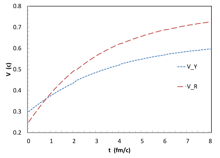
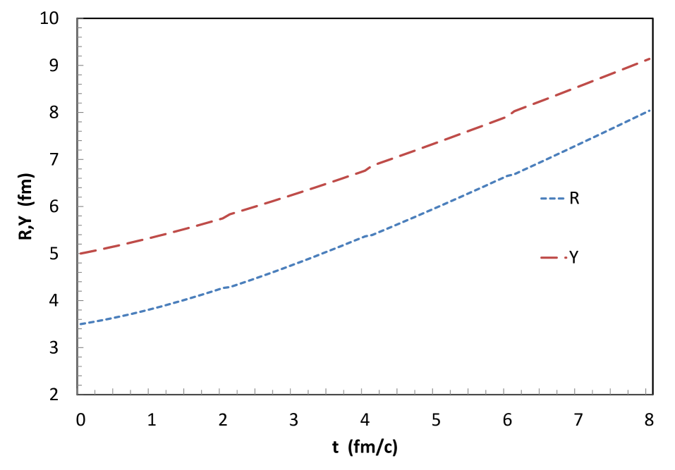
Figure 2: (Color online) Left: The time dependence of the velocity of expansion in the transverse radial direction, $v_{R}$ and in the direction of the axis of the rotation, $v_{Y}$ for the configuration shown in Fig. 1. The expansion velocity is increasing in both directions. While in the axis direction the velocity increases from 0.3 c to 0.6 c in 8 fm/c time, the radial expansion increases faster, in part due to the centrifugal force from the rotation. Right: The time dependence of the Radial, $R$, and axis directed, $Y$, size of the expanding system. As the $Y$ directed velocity is initially larger its change is relatively smaller.

As the exact solution is able to describe the monotonic expansion, and so the steady decrease of the rotation, we start from a higher initial angular velocity than shown by the fluid dynamical model, PICR, as the angular velocity, measured versus the horizontal plane, starts from zero.

Applying these initial parameters the exact model yields a dynamical development shown in Table 1. According to expectations the radius, $R$, and the axis directed size, $Y$, are increasing, the angular velocity, $\omega$ decreases, The total energy is conserved, while the kinetic energy of expansion is increasing, and that of the rotation and internal energy are decreasing. See Fig. 1.

The change of the expansion velocity, $v_{R}=\dot{R}$, is shown in Fig. 2 left. The more rapid velocity change arises partly from the centrifugal acceleration of the rotation, but also from the fact that the initially smaller transverse size increases faster in the direction of equal sizes in both directions. See Fig. 2 right.

The study of the rotation in an infinite system is. on the other hand, problematic as we assume solid body rotation (i.e. the angular momentum applies to the whole infinite system). So the applicability of this infinite model to a heavy ion reaction is highly approximate, and the external tails should be disregarded.

Other finite scaling expansion profiles can also be studied, based on the given examples, and these may fit more detailed fluid dynamical models better.

5 The vorticity

In the usual convention in heavy ion physics, the beam axis is the $z$ axis, the impact parameter vector, $b$, points in the $x$ direction, and the projectile is at positive $x$ and moves in the positive $z$ direction. Thus the rotation axis is the $y$ axis, this is the axis of the cylindrical symmetry of the rotating exact model system we discussed above. The reaction plane $x,z$ is spanned by the cylindrical coordinates $r,\varphi$ in the discussion above.

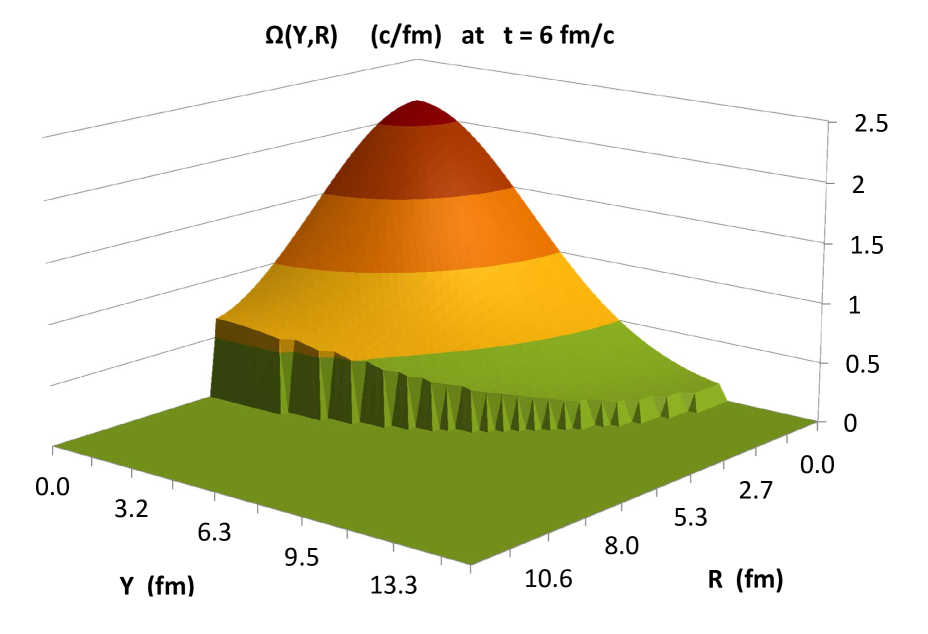
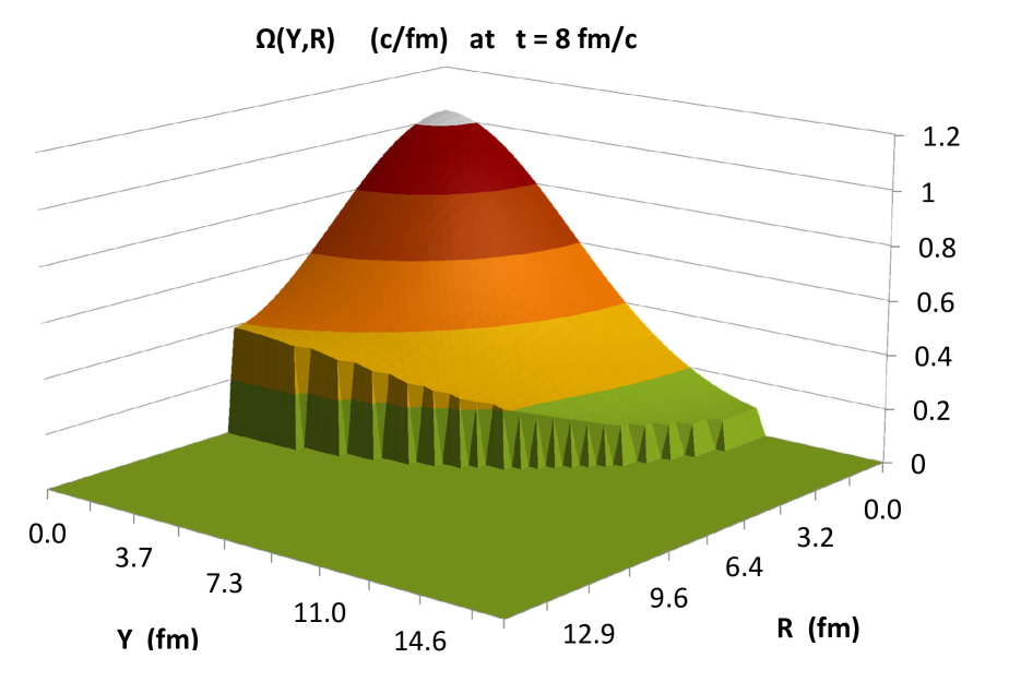
Figure 3: (Color online) The energy weighted vorticity in the classical rotating exact model with Gaussian density profiles, with an EoS of $\kappa=3/2$, and with initial parameters: 3.5 fm mean radius, 5.0 fm mean length, 0.1 c/fm angular velocity, 0.25 c radial velocity, 0.3 c axis directed velocity ($v_{y}$). The initial temperature of the matter is $T=400$ MeV. The figures show the configuration at different times. At $t=2$ fm/c, the mean radial (longitudinal) sizes and speeds are 4.27 fm (5.75 fm) and 0.494 c (0.437 c), and the angular velocity is 0.07 c/fm. The $v=c$-boundary is at $Y_{max}=11.0$ fm and $R_{max}=6.3$ fm. At $t=4$ fm/c, the mean radial (longitudinal) sizes and speeds are 5.67 fm (6.76 fm) and 0.62 c (0.52 c), and $\omega=0.04$ c/fm. The $v=c$-boundary is at $Y_{max}=7.1$ fm and $R_{max}=11.1$ fm. At $t=6$ fm/c, the mean radial (longitudinal) sizes and speeds are 6.65 fm (7.91 fm) and 0.69 c (0.57 c), and $\omega=0.0$ c/fm. The $v=c$-boundary is at $Y_{max}=12.0$ fm and $R_{max}=7.98$ fm. At $t=8$ fm/c, the mean radial (longitudinal) sizes and speeds are 8.04 fm (9.14 fm) and 0.73 c (0.60 c), and $\omega=0.02$ c/fm. The $v=c$-boundary is at $Y_{max}=13.16$ fm and $R_{max}=9.32$ fm.

For rotation around the y-axis the vorticity is defined in terms of the velocity field as $\omega_{y}=(\partial_{z}v_{x}-\partial_{x}v_{z})/2$. We use the conventions of the exact model here, so that we chose the rotation axis to be the $y$ axis and the plane of the rotation is the $x,z$ plane, which corresponds to the reaction plane. We assume that the rotating system is symmetric, so we introduce cylindrical coordinates around the rotation axis.

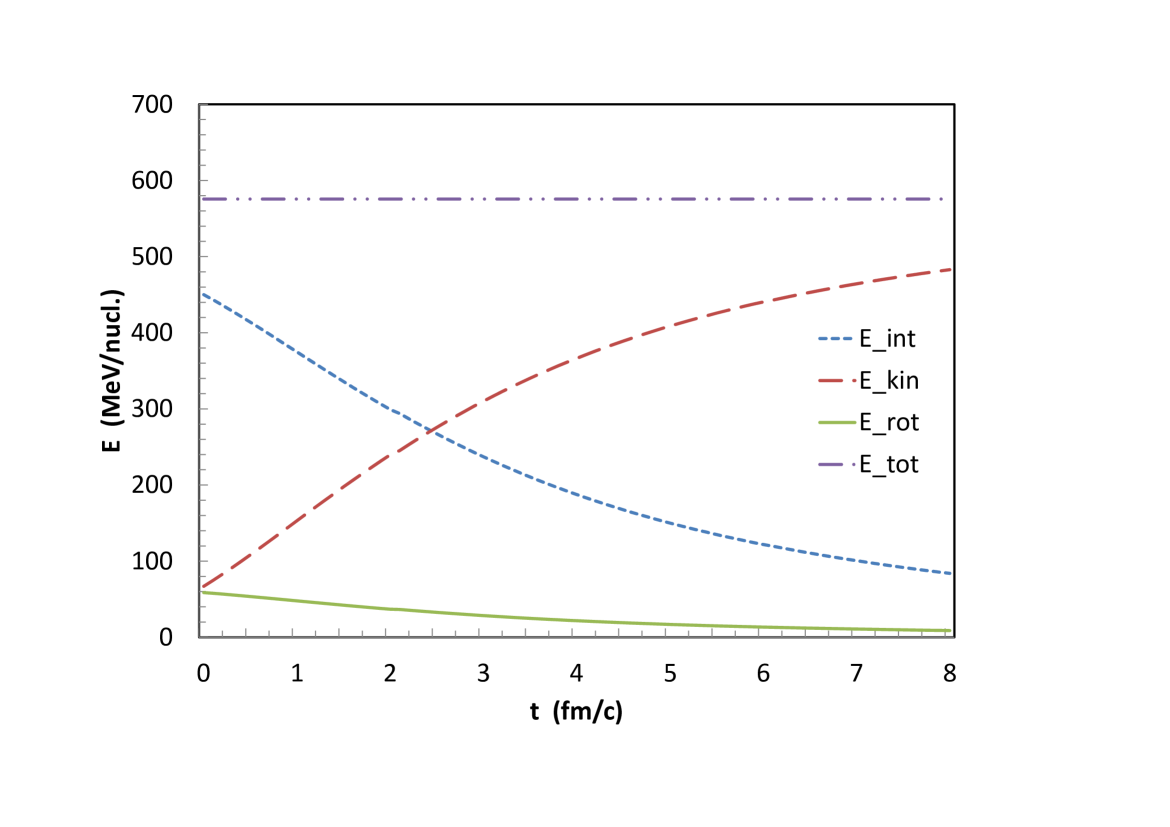
Figure 4: (Color online) The time dependence of the kinetic energy of the expansion, $E_{kin}$, the internal energy, $E_{int}$, the rotational energy, $E_{rot}$, and the total energy, $E_{tot}$ per nucleon in the exact model with the initial conditions $R_{0}$ = 2.5 fm, $Y_{0}$ = 4.0 fm, $\dot{R}_{0}$ = 0.20 c, $\dot{Y}_{0}$ = 0.25 c, $\omega_{0}$ = 0.1 c/fm, $\kappa=3/2$, $T_{0}$ = 300 MeV. For this configuration $E_{tot}=576$ MeV/nucl. The kinetic energy of the expansion is increasing, at the cost of the decreasing internal energy and the slower decreasing rotational energy. The rotational energy is decreasing to the half of the initial one in 2.9 fm/c.

For this configuration in cylindrical coordinates the vorticity is .

$$\omega \equiv {\rm rot}\mbox{\boldmath$v$}$$ (26)

$$= \left(\frac{1}{\rho}\frac{\partial v_{y}}{\partial\varphi}-\frac{\partial v_{\varphi}}{\partial y}\right)\mbox{\boldmath$e$}_{\rho}+\left(\frac{\partial v_{\rho}}{\partial y}-\frac{\partial v_{y}}{\partial\rho}\right)\mbox{\boldmath$e$}_{\varphi}+\left(\frac{1}{\rho}\frac{\partial(\rho v_{\varphi})}{\partial\rho}-\frac{1}{\rho}\frac{\partial v_{\rho}}{\partial\varphi}\right)\mbox{\boldmath$e$}_{y}$$

$$= -2\omega\mbox{\boldmath$e$}_{y}\,.$$

At the last step we use Eq. (5), where $v_{y}$ does not depend on $\varphi$, $v_{\varphi}$ does not depend on $y$, $v_{\rho}$ does not depend on $y$, $v_{y}$ does not depend on $\rho$ and $v_{\rho}$ does not depend on $\varphi$, thus only one term contributes to the vorticity, which is directed in the direction of $\mbox{\boldmath$e$}_{y}$.

Thus the vorticity in this model is spatially homogeneous, and depends on the time only, $\omega=\omega(t)$. However, from the point of view of observations, it is important what amount of energy or mass is representing a given fluid element with the given vorticity. In the solution we presented here we assumed a uniform temperature, which led to a gaussian density and energy profile, $\epsilon(\rho)=\kappa Tn(\rho)$.

Following reference [2], we define an energy-density-weighted, average vorticity as

$$\Omega_{zx}\equiv w(r_{\rho},r_{\phi},r_{y})\,\omega$$ (27)

so that this weighting does not change the average circulation of the layer, i.e., the sum of the average of the weights over all fluid elements is unity, $\langle w(z,x)\rangle=1$. This weighting does not change the average vorticity value of the set; just the cells will have larger weight with more energy content.

Let us fist calculate the internal energy for a finite system:

$$E_{int}=\int_{-aY}^{+aY}\int_{0}^{bR}\epsilon(r_{\rho},r_{y})\ 2\pi r_{\rho}dr_{\rho}dr_{y}\ ,\\$$

while the the energy at a given radius (at a given time) is $\epsilon(r_{\rho},r_{y})$. Thus the weight density will be

$$w(r_{\rho},r_{\phi},r_{y})=\frac{T^{00}(r_{\rho},r_{y})}{E_{tot}/V}\ ,$$ (28)

where

$$T^{00}=\epsilon\left[(1+1/\kappa)\ \gamma^{2}-1/\kappa\right]\ \ \ \ {\rm and}$$

$$\epsilon(r_{\rho},r_{y}) = \kappa n_{0}\frac{V_{0}}{V}T_{0}\left(\frac{V_{0}}{V}\right)^{1/\kappa}\mathcal{T}(s)e^{-\frac{1}{2}\int_{0}^{s}\frac{du}{\mathcal{T}(u)}}$$ (29)

$$= \kappa T_{0}n_{0}\left(\frac{V_{0}}{V}\right)^{1+1/\kappa}e^{-s_{y}/2}e^{-s_{\rho}/2},$$

while $\gamma^{2}=\left[1-\left(\frac{\dot{R}}{R}r_{\rho}\right)^{2}-\left(\omega r_{\rho}\right)^{2}-\left(\frac{\dot{Y}}{Y}r_{y}\right)^{2}\right]^{-1}$. Here we assumed that $\mathcal{T}(s)=1$ and let $C=\kappa n_{0}\frac{V_{0}}{V}T_{0}\left(\frac{V_{0}}{V}\right)^{1/\kappa}$ to get $\epsilon(r_{\rho},r_{y})=Ce^{-s/2}$. With $s=s_{\rho}+s_{y}$ where $s_{\rho}=r_{\rho}^{2}/R^{2}$ and $s_{y}=r_{y}^{2}/Y^{2}$.

We also get that

$$E_{int}=C\int_{-aY}^{+aY}e^{-\frac{r_{y}^{2}}{2Y^{2}}}dr_{y}\int_{0}^{bR}e^{-\frac{r_{\rho}^{2}}{2R^{2}}}2\pi r_{\rho}dr_{\rho}\ .$$

Using a change of variables to $s_{y}$ and $s_{\rho}$, so that $dr_{y}=\frac{Y}{2\sqrt{s_{y}}}ds_{y}$ and $2\pi r_{\rho}\,dr_{\rho}=R^{2}\pi ds_{\rho}$, the scaling integration boundaries will be $S_{yM}=a^{2},\ \$ $S_{\rho M}=b^{2}$ and we find

$$E_{int}=C\pi R^{2}Y\int_{-a^{2}}^{+a^{2}}e^{-s_{y}/2}\frac{ds_{y}}{\sqrt{s_{y}}}\int_{0}^{b^{2}}e^{-s_{\rho}/2}\,ds_{\rho}\ .$$

We can express the integrals as follows

$$2\,I_{A}(b^{2}/2)\equiv\int_{0}^{b^{2}}e^{-s_{\rho}/2}ds_{\rho}=2\int_{0}^{b^{2}/2}e^{-u}du$$

and

$$2\sqrt{2}\,I_{B}(a^{2}/2)\equiv\int_{-a^{2}}^{a^{2}}e^{-s_{y}/2}\frac{ds_{y}}{\sqrt{s_{y}}}=2\int_{0}^{a^{2}}e^{-s_{y}/2}\frac{ds_{y}}{\sqrt{s_{y}}}=2\sqrt{2}\int_{0}^{a^{2}/2}e^{-u}\frac{du}{\sqrt{u}}\ ,$$

where

$$I_{A}(u)=1-e^{-u},\ \ \ {\rm and}\ \ \ I_{B}(u)=\sqrt{\pi}\Phi(\sqrt{u})\ .$$

Thus

$$E_{int} = C\pi R^{2}Y2I_{A}(b^{2}/2)2\sqrt{2}I_{B}(a^{2}/2)$$ (30)

$$= C\pi R^{2}Y4\sqrt{2}\left(1{-}e^{-b^{2}/2}\right)\sqrt{\pi}\ \Phi\left(a/\sqrt{2}\right).\$$

Similarly we can calculate the Kinetic energies, $E_{kin}$, for the rotation and radial and longitudinal expansions as in [8] (and see the Appendix). Then, using Eq. (11) or (17), the total energy of the system is

$$E_{tot}=E_{int}+E_{kin}\ ,$$ (31)

which we can use in the calculation of the weighted vorticity.

In the present study we assumed an infinite system with scaling gaussian density profile, Eq. (12), so that the integrals are evaluated up to infinity.

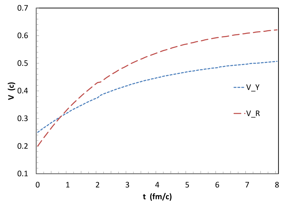
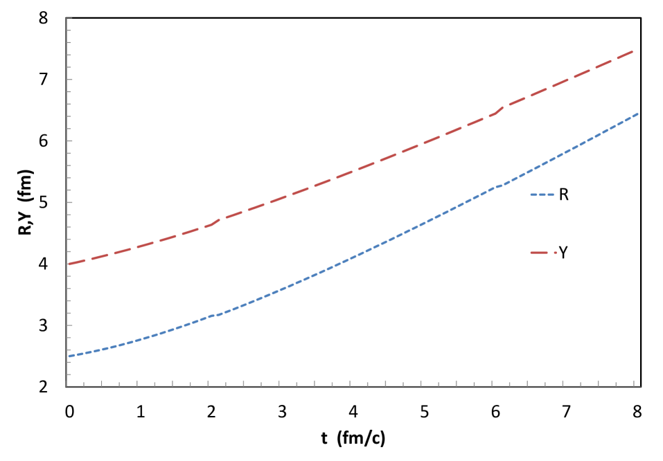
Figure 5: (Color online) Left: The time dependence of the velocity of expansion in the transverse radial direction, $v_{R}$ and in the direction of the axis of the rotation, $v_{Y}$, for the configuration presented in Fig. 4. The expansion velocity is increasing in both directions. While in the axis direction the velocity increases from 0.25 c to 0.5 c in 8 fm/c time, the radial expansion increases faster. Right: The time dependence of the Radial, $R$, and axis directed, $Y$, size of the expanding system.

6 Results and Discussion

We performed a set of calculations to study the applicability of the model to heavy ion reactions. This presented non-relativistic model leads to super-luminous velocities at late times and at the external surface of the system. We used a parametrization where the peripheral energy density is cut off exponentially, and took initial conditions such that the vast majority of the system is in the non-relativistic applicable domain of the model.

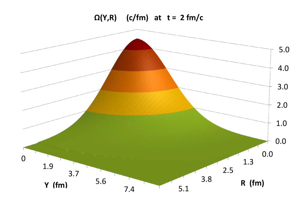
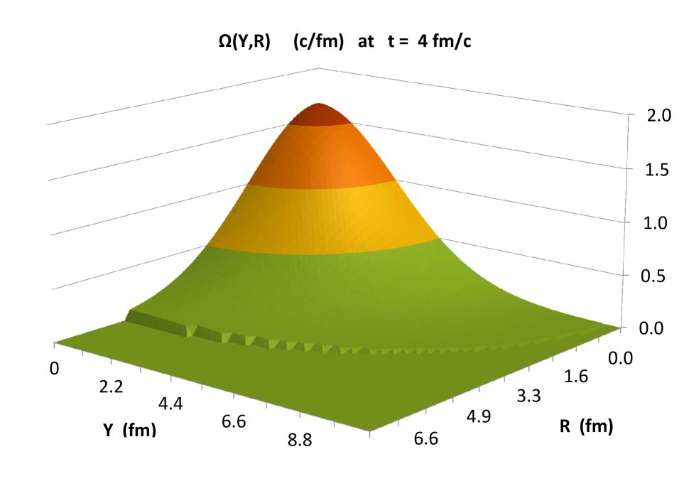
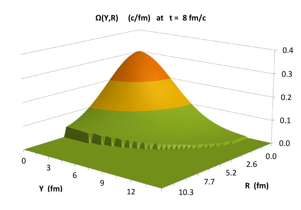
Figure 6: (Color online) The energy weighted vorticity in the classical rotating exact model with Gaussian density profiles, with initial parameters as given in Fig. 4. The figure shows the configuration at $t=2$ fm/c, when the mean radial (longitudinal) sizes and speeds are 3.16 fm (4.64 fm) and 0.43 c (0.38 c), and the angular velocity is 0.06 c/fm. The boundary is at the position where the velocity of matter reaches the speed of light, c. This happens at $Y_{max}>9.0$ fm and $R_{max}=5.68$ fm. At $t=4$ fm/c, the mean radial (longitudinal) sizes and speeds are 4.11 fm (5.51 fm) and 0.54 c (0.45 c), and $\omega=0.04$ c/fm. The $v=c$-boundary is at $Y_{max}=10.58$ fm and $R_{max}=6.24$ fm. At $t=6$ fm/c, the mean radial (longitudinal) sizes and speeds are 5.25 fm (6.45 fm) and 0.59 c (0.48 c), and $\omega=0.02$ c/fm. The $v=c$-boundary is at $Y_{max}=11.34$ fm and $R_{max}=7.56$ fm. At $t=8$ fm/c, the mean radial (longitudinal) sizes and speeds are 6.44 fm (7.49 fm) and 0.62 c (0.51 c), and $\omega=0.02$ c/fm. The $v=c$-boundary is at $Y_{max}=12.58$ fm and $R_{max}=8.75$ fm.

A first series of calculations is presented in Figs. 3.

With the parameters as defined in Figs. 3 when we reach $t=8$ fm/c the surface speed reaches the speed of light already when the Energy weighted vorticity drops to 40% of the top central value. Thus, a substantial amount of matter is outside the range of physical applicability of the model. The evaluation of polarization would not be realistic with these sets of parameters. Therefore we modified our initial conditions such that the applicability of the non-relativistic model holds up to the final, freeze out time of about 8 fm/c.

The time development of the change of the different forms of energy are presented in Fig. 4, for the modified initial state, While the sizes $R$ and $Y$, and the expansion velocities in these directions are shown in Fig. 5.

Now the total energy of the system is about 70% of the previous example, and the initial rotational energy is 60% of the previous one.

We also performed another test series with this more compressed initial state configuration 6. While up to $t=6$ fm/c the majority of the energy weighted vorticity is in the applicable domain (where the velocity does not exceed the velocity of light), at $t=8$ fm/c roughly 95% of the energy content is still in the applicability domain of the non-relativistic exact model (see Fig. 6). We may estimate that about 50-70% of the initial energy of a peripheral collision will contribute to the expansion of an symmetric solution of our participant system. Thus the model is applicable at lower energies, FAIR and NICA, energies, while at the top energies of RHIC or LHC the reliability of this model is qualitative, and may provide estimates with 15 - 20 % accuracy.

7 Conclusions

The effect of QGP formation on the directed flow and the arising 3rd flow component or antiflow was first observed in fluid dynamical calculation at energies above 10 GeV per nucleon in Ref. [15]. The nuclear EoS has to satisfy strong constraints from the observed Neutron and Hybrid Star masses [16] Spin-orbit interaction and the momentum dependence of the nuclear interaction [17], influence the nuclear EoS and developing rotation and polarization of the participant matter. The nuclear EoS has a strong effect on the collective motion. Transverse flow and collectivity was observed early both in fluid dynamical, nuclear cascade and molecular dynamics models [18].

In conclusion, the exact model can be well realized with parameters extracted from detailed, high resolution, 3+1D relativistic fluid dynamical model calculations with the PICR code. It provides an estimate of the rate of decrease of angular speed and rotational energy due to the expansion in an explosively expanding system. This indicates that the effects of rotation can be observable in case of rapid freeze out and hadronization, although the Kelvin Helmholtz Instability is not present in this model and this reduces the rotation at later times.

This indicates that the presence of the KHI is essential for an observable effect of the rotation, and thus the observation of the rotation is strongly connected to the evolving turbulent instability in low viscosity Quark-gluon plasma.

References

8 Appendix - Scaling of density distributions

Let us evaluate the baryon density, $n(s)$, and for simplicity let us assume that in case 1A of Ref. [10] the temperature is constant, $\mathcal{T}(s)=1$, then it follows that, $\nu(s)=(N_{B}/V)\exp(-s/2)$, where $N_{B}=n_{0}\,V_{0}$. Due to the exponential density profile, if $s$ is a sum of the coordinates in two orthogonal directions, as $s=s_{\rho}=s_{z}$, then n(s) separates into two multiplicative terms: $n_{\rho}(s_{\rho})$ and $n_{z}(s_{z})$. For further simplifying the formalism, we can introduce a coordinate change $s=2u$ for integrals of type $\int_{0}^{U/2}f(u/2)\,du$. Then $ds=2\,du$ and $2\int_{0}^{U/2}f(u/2)\,du=\int_{0}^{S}f(s)\,ds$. This change will thus modify the upper limits of integration, and the normalization by a factor of two. These adjustments are included in the final expressions in Appendices 8-11.

The baryon density distribution is then

$$n(r_{\rho},r_{y})=N_{B}\frac{C_{n}}{V}e^{-r_{\rho}^{2}/R^{2}}e^{-r_{y}^{2}/Y^{2}}$$

where $C_{n}$ is a normalization constant, which will be determined later. The normalization can be performed up to a finite size, $R$ and $Y$, or up to infinity.

$$\int\!\!\!\int\!n(r_{\rho},r_{y}) = N_{B}\frac{C_{n}}{V}$$

$$2\pi \times \int_{0}^{R/\infty}e^{-r_{\rho}^{2}/R^{2}}r_{\rho}dr_{\rho}$$ (32)

$$\times \int_{-Y/\infty}^{Y/\infty}e^{-r_{y}^{2}/Y^{2}}dr_{y}\ ,$$

here the first integral up to infinity gives $\Gamma(1)R^{2}/2$, while the second one $\Gamma(0.5)Y=\sqrt{\pi}Y$. In $x,\,y,\,z$ coordinates this is:

$$N_{B}\frac{C_{n}}{V} \times \left(\int_{-\infty}^{\infty}e^{-r_{x}^{2}/\dot{R}^{2}}dr_{x}\right)^{3}=$$

$$N_{B}\frac{C_{n}}{V}\left(\sqrt{\pi}\dot{R}\right)^{3} = N_{B}\times{\rm const.}$$ (33)

Or in cylindrical coordinates

$$N_{B}\frac{C_{n}}{V} \times \pi\Gamma(1)R^{2}\times\sqrt{\pi}Y=N_{B}\frac{C_{n}}{V}\pi^{3/2}R^{2}Y\ ,$$ (34)

which is the same. The integrals were evaluated up to limits in infinity. If we perform the definite integrals up to a finite limit, we get similar scaling behaviour. Let us now change the variables to scaling variables introduced in Ref. [10], but in cylindrical coordinates.

$$n(s_{\rho},s_{y})=N_{B}\frac{C_{n}}{V}\,e^{-s_{\rho}/2}\,e^{-s_{y}/2}.$$

Now using the relations $2\pi r_{\rho}dr_{\rho}=\pi R^{2}ds_{\rho}$ and $dr_{y}=\frac{Y}{2\sqrt{s_{y}}}ds_{y}$ we get

$$\int\!\!\!\int\!n(s_{\rho},s_{y}) = N_{B}\frac{C_{n}}{V}$$

$$\times \pi R^{2}\!\!\int_{0}^{1}\!\!e^{-s_{\rho}/2}\,ds_{\rho}\times Y\!\!\int_{0}^{1}\!\!e^{-s_{y}/2}\,\frac{ds_{y}}{\sqrt{s_{y}}}=$$

$$N_{B}{C_{n}}\frac{\pi R^{2}Y}{V} \times 2\!\!\int_{0}^{0.5}\!\!e^{-u}\,du\times\sqrt{2}\!\!\int_{0}^{0.5}\!\!e^{-u}\,\frac{du}{\sqrt{u}}$$ (35)

$$= N_{B}C_{n}\frac{\pi R^{2}Y}{V}\ 2\,I_{A}(0.5)\ \sqrt{2}\,I_{B}(0.5)$$

This should be equal to $N_{B}$ thus the normalization constant is

$$C_{n}=1\left/\left[2\sqrt{2}\,I_{A}(0.5)\,I_{B}(0.5)\right]\right..$$

Here $I_{A}(0.5)$ and $I_{B}(0.5)$ are constants, which do not change during the scaling evolution, when the density profile remains the same. At infinity $I_{A}(\infty)=\Gamma(1)$ while $I_{B}(\infty)=\Gamma(0.5)=\sqrt{\pi}$, but at different integration limits the ratio of the two integrals will be different [12]:

$$I_{A}(u) = 1-\exp(-u)$$

$$I_{B}(u) = \sqrt{\pi}\,\Phi(\sqrt{u}\,)\ ,$$ (36)

where

$$\Phi(u)={\rm erf}(u)\equiv\frac{2}{\sqrt{\pi}}\int_{0}^{u}\exp(-x^{2})\,dx\ .$$ (37)

9 Appendix - The Moment of Inertia

Consider a body with scaling expansion, and with solid body rotation (i.e. the angular velocity is uniform for the whole body, $\omega=\omega(t)$ but it does not depend on the spatial coordinates. Let us denote the moment of inertia with $\Theta$,

$$\Theta=\int m\,n(r)\,r^{2}\,d^{3}r\ .$$ (38)

Then the angular momentum and the rotational energy are

$$L=\Theta\omega\ \ \ {\rm and}\ \ \ E=\frac{1}{2}\Theta\omega^{2}\ .$$ (39)

Now we assume that our system has no external torque, and all internal forces are radial, so the angular momentum must be conserved, during the scaling expansion driven by the pressure gradient which is radial in a cylindrically symmetric system. Thus, the angular velocity is not directly influenced by the dynamics, just via the angular momentum conservation. From $\dot{L}=0\ ,$ it follows that

$$\dot{\Theta}\omega=-\Theta\dot{\omega}\ \ \ {\rm or}\ \ \ \dot{\omega}=-\omega\frac{\dot{\Theta}}{\Theta}\ .$$

Thus the change of the angular velocity is a direct consequence of the change of the moment of inertia $\Theta$, while $\Theta$ is proportional with the square of the radius of the system in a scaling expansion where the density profile remains the same during the expansion. Consequently

$$\dot{\omega}\ =\ -\omega\frac{\dot{\Theta}}{\Theta}\ =\ -\omega\frac{\dot{R}^{2}}{R^{2}}\ \ \ {\rm and}\ \ \ \omega\ =\ \omega_{0}\frac{R_{0}}{R}\ .$$

We still have to evaluate the moment of inertia accurately to provide precisely the energy of rotation. Thus, using the scaling variables

$$\Theta = mN_{B}\frac{\pi R^{2}\,Y}{V}R^{2}C_{n}\!\!\int_{0}^{1}\!\!e^{-s_{\rho}/2}s_{\rho}ds_{\rho}\times\!\!\int_{0}^{1}\!\!e^{-s_{y}/2}\frac{ds_{y}}{\sqrt{s_{y}}}$$ (40)

$$= m\,N_{B}\,R^{2}\ C_{n}\ 4\,I_{C}(0.5)\,\sqrt{2}\,I_{B}(0.5)\ ,$$

where $I_{C}(u)=1-(1+u)\exp(-u)\ .$

As before these integrals do not change during the scaling expansion, on the other hand the volume and the moment of inertia have different coefficients in the energy expression. As a consequence the kinetic energy of the rotation is

$$E_{kin} = \frac{1}{2}\Theta\omega^{2}=\frac{1}{2}m\,N_{B}\ C_{n}4\sqrt{2}\,I_{C}(0.5)\,I_{B}(0.5)\,R^{2}\omega^{2}$$ (41)

$$= \frac{1}{2}\alpha^{2}\,m\,N_{B}\ R^{2}\omega^{2}\ .$$

Here we have introduced the constant

$$\alpha^{2}\equiv 4\sqrt{2}\,C_{n}I_{B}({\small\frac{1}{2}})I_{C}({\small\frac{1}{2}}),$$ (42)

that can be used in the main course of the work.

10 Appendix - Kinetic energy of radial expansion

The radial velocity is given by $v_{\rho}=(\dot{R}/R)r_{\rho}$ and consequently $v_{\rho}^{2}=\dot{R}^{2}s_{\rho}$. Thus the kinetic energy of radial expansion is

$$E_{kin} = \frac{mN_{B}}{2}\frac{\pi R^{2}Y}{V}\dot{R}^{2}C_{n}\int_{0}^{1}\!\!\!e^{-s_{\rho}/2}s_{\rho}ds_{\rho}\int_{0}^{1}\!\!\!e^{-s_{y}/2}\frac{ds_{y}}{\sqrt{s_{y}}}$$ (43)

$$= \frac{mN_{B}}{2}C_{n}4\sqrt{2}\,I_{C}(0.5)\,I_{B}(0.5)\ \dot{R}^{2}$$

$$= \frac{mN_{B}}{2}\,\alpha^{2}\ \dot{R}^{2}$$

11 Appendix - Kinetic energy of longitudinal expansion

The longitudinal velocity is given by $v_{y}=(\dot{Y}/Y)r_{y}$ and consequently $v_{y}^{2}=\dot{Y}^{2}s_{y}$. Thus the kinetic energy of longitudinal expansion is

$$E_{kin} = \frac{mN_{B}}{2}\frac{\pi R^{2}Y}{V}\dot{Y}^{2}C_{n}\!\!\int_{0}^{1}\!\!\!e^{-s_{\rho}/2}ds_{\rho}\int_{0}^{1}\!\!\!e^{-s_{y}/2}\sqrt{s_{y}}ds_{y}$$ (44)

$$= \frac{mN_{B}}{2}C_{n}\ 4\sqrt{2}\,I_{A}(0.5)\,I_{D}(0.5)\ \dot{Y}^{2}\ ,$$

where $I_{D}(u)=\frac{\sqrt{\pi}}{2}\Phi(\sqrt{u})-\sqrt{u}e^{-u}.$ Here we can introduce the constant

$$\beta^{2}\equiv 4\sqrt{2}\,C_{n}I_{A}({\small\frac{1}{2}})I_{D}({\small\frac{1}{2}}),$$ (45)

which will be used in the calculation.

12 Appendix - Not realizable analytic solution.

One may find a solution for the dynamical evolution of $R(t)$ and $Y(t)$ based on Eq. 16, with simplifying the problem to a singe, first order differential equation in a similar way as it is done in Ref. [13]. Let us introduce a parametric function, $\phi(t)$,

$$\alpha R(t) = U(t)\sin\phi(t)$$

$$\beta Y(t) = U(t)\cos\phi(t)\ ,$$ (46)

satisfying Eq. (19). Now inserting Eqs. (46) into Eq. (16), and noticing that $\alpha^{2}\dot{R}^{2}+\beta^{2}\dot{Y}^{2}=\dot{U}^{2}+U^{2}\dot{\phi}^{2}$ we get the following first order differential equation for $\phi$:

$$\dot{\phi}^{2}=\frac{1}{U^{2}(t)}\!\!\!\left[\ {\cal F}-\,\dot{U}^{2}(t)-\,\frac{\alpha^{4}W}{U^{2}(t)\sin^{2}\phi}-\,\frac{(\alpha^{2}+\beta^{2})(\alpha^{2}\,\beta)^{\gamma}Q}{(\pi U^{3}(t)\sin^{2}\phi\cos\phi)^{\gamma}}\ \right].$$ (47)

The initial value of the variable $\phi$ is chosen such that Eq. (46) is satisfied for $U(t_{0}),\ \phi(t_{0})$.

The problem with this solution is that Eq. (47) describes the square of $\dot{\phi}$ and in a realistic situation it is not trivial to find the sign of the r.h.s. of the dynamical equation for $\dot{\phi}$. This sign alternates.

References

[1]
J. H. Gao, Z. T. Liang, S. Pu, Q. Wang
and X. N. Wang, Phys. Rev. Lett. 109, 232301 (2012).
[2]
L.P. Csernai, V.K. Magas, D.J. Wang, Phys. Rev. C 87,
034906 (2013).
[4]
L.P. Csernai, V.K. Magas, H. Stöcker, and D.D. Strottman,
Phys. Rev. C 84, 024914 (2011).
[5]
L.P. Csernai, D.D. Strottman and Cs. Anderlik,
Phys. Rev. C 85, 054901 (2012).
[6]
D.J. Wang, Z. Néda, and L.P. Csernai,
Phys. Rev. C 87, 024908 (2013)
[7]
L.P. Csernai, and J.I. Kapusta,
Phys. Rev. D 31, 2795 (1985).
[8]
L.P. Csernai, D.J. Wang and T. Csörgő,
Phys. Rev. C 90, 024901 (2014).
[9]
Y. Hatta, J. Noronha, Bo-Wen Xiao,
Phys. Rev. D 89, 051702 (2014).
[10]
T. Csörgő and M.I. Nagy,
Phys. Rev. C 89, 044901 (2014).
[11]
Horst Stöcker: Taschenbuch Der Physik,
(Harri Deutsch, 2000), 1.3.2/6d.
[12]
M. Abramowitz, and I.A. Stegun: Handbook of mathematical functions
(Dover, New York, 1965) 6.5.2;
I.S. Gradstein, and I.M. Ryzhik: Table of Integrals …,
(Academic Press, 1994)
3.321/2., 3.361/1., 3.381/1., 8.250/1., 8.251/1., 8.350/1., 8.354/1.
[13]
S.V. Akkelin, T. Csörgő, B. Lukács, Yu. M. Sinyukov, and
M. Weiner, Phys. Lett. B 505 (2001) 64-70.
[14] W.E. Boyce and R.C. DiParma: Elementary Differential Equations and Boundary Value Problems,
(Wiley, 1997).
[15]
L.V. Bravina, N.S. Amelin, L.P. Csernai, P. Lévai, and D. Strottman,
Nuclear Physics A 566, 461-464 (1994).
[16]
A. Rosenhauer, E.F. Staubo, L.P. Csernai, T. Overgard, and E. Ostgaard,
Nucl. Phys. A 540, 630 (1992).
[17]
L.P. Csernai, G. Fai, C. Gale, and E. Osnes,
Phys. Rev. C 46, 736 (1992).
[18]
N.S. Amelin, E.F. Staubo, L.P. Csernai, V.D. Toneev, K.K. Gudima, and
D. Strottman,
Phys. Rev. Lett. 67, 1523 (1991).