Local principle satisfying high order total variation diminishing approximation for non-sonic data extrema

Abstract

The main contribution of this work is to construct higher than second order accurate total variation diminishing (TVD) schemes which can preserve high accuracy at non-sonic extrema with out induced local oscillations. It is done in the framework of local maximum principle (LMP) and non-conservative formulation. The representative uniformly second order accurate schemes are converted in to their non-conservative form using the ratio of consecutive gradient. These resulting schemes are analyzed for their non-linear LMP/TVD stability bounds using the local maximum principle. Based on the bounds, second order accurate hybrid numerical schemes are constructed using a shock detector. Numerical results are presented to show that such hybrid schemes yield TVD approximation with second or higher order convergence rate for smooth solution with extrema.

keyword Hyperbolic conservation laws;Smoothness parameter; Non-sonic critical point, Total variation stability, Finite difference schemes.
AMS Classification: 65M12, 35L65,35L67,35L50,65M06,65M15 65M22.

1 Introduction

We consider the 1D scalar conservation law associated to the conserved variable $u(x,t)$,

$$\displaystyle\frac{\partial}{\partial t}u(x,t)+\frac{\partial}{\partial x}f(u(x,t))=0,\;\;(x,\,t)\in\mathbb{R}\times\,\mathbb{R}^{+}$$ (1)

$$u(x,0)=u_{0}(x)$$

where $f(u)$ is a non-linear flux function. The numerical approximation for the solution of (1) is done by the discretization of the spatial and temporal space into $N$ equispaced cells $I_{i}=[x_{i-\frac{1}{2}},x_{i+\frac{1}{2}}],\;i=0,1,\dots N$ of length $\Delta x$ and $M$ equispaced intervals $[t^{n},t^{n+1}],\;n=0,1,\dots,M$ of length $\Delta t$ respectively. Let $x_{i}=i\Delta x$ and $t^{n}=n\Delta t$ denote the cell center of cell $I_{i}$ and the $n^{th}$ time level respectively then a conservative numerical approximation for (1) can be defined by

$${u}^{n+1}_{i}={u}_{i}^{n}-\lambda\left(\mathcal{F}^{n}_{i+\frac{1}{2}}-\mathcal{F}^{n}_{i-\frac{1}{2}}\right),\;\;\lambda=\frac{\Delta t}{\Delta x}.$$ (2)

where ${u^{n}_{i}=u(x_{i},t^{n})}$ and $\mathcal{F}^{n}_{i\pm\frac{1}{2}}$ is the numerical flux function defined at the cell interface $x_{i\pm\frac{1}{2}}$ at time level $n$. The characteristics speed $a(u)=\frac{\partial f(u)}{\partial u}$ associated with (1) can be approximated as,

$$a^{n}_{i+\frac{1}{2}}=\left\{\begin{array}[]{clc}\displaystyle\frac{F^{n}_{i+1}-F^{n}_{i}}{{u}^{n}_{i+1}-{u}^{n}_{i}}&\mbox{if}&{u}^{n}_{i+1}\neq{u}^{n}_{i},\\ &&\\ \displaystyle\left.\frac{\partial f}{\partial u}\right|_{{u}^{n}_{i}}&\mbox{if}&{u}^{n}_{i+1}={u}^{n}_{i}\end{array}\right.,$$ (3)

where $F_{i}=f(u^{n}_{i})$. In general due to non-linearity of (1), beyond a small finite time, even for a smooth initial data the evolution of discontinuities in the solution $u(x,t)$ is inevitable. Therefore, it is required to have a conservative approximation of the solution with high accuracy and crisp resolution of such discontinuities with out numerical oscillations. Contrary to this need, most classical high order schemes despite of being linearly Von-Neumann stable give oscillatory approximation for discontinuities even for the trivial case of transport equation i.e., $f(u)=au,\,0\neq a\in R$. Such oscillatory approximation can not be considered as admissible solution since it violets the following global maximum principle satisfied by the physically correct solution $u(x,t)$ of (1) i.e.,

$$\min(u_{0}(x))\leq u(x,t)\leq\max(u_{0}(x)),\forall(x,\;t)\in\mathbb{R}\times\,\mathbb{R}^{+}.$$ (4)

In order to overcome these undesired numerical instabilities, various notion of non-linear stability are developed in the light of maximum principle (4). Examples of Maximum principle satisfying schemes are monotone schemes [42, 4], total variation diminishing (TVD) schemes [13, 38, 45, 34, 5, 10, 16, 47]. Some uniformly high order maximum-principle satisfying and positivity preserving schemes are [21, 48, 46]. There are other non-oscillatory schemes which do not strictly follow maximum principle but practically give excellent numerical results e.g., Essentially non-oscillatory (ENO) and weighted ENO schemes see [35] and references therein. It is known that among global maximum principle satisfying schemes, the monotone and total variation diminishing (TVD) schemes experience difficulties at data extrema. On the one hand, such high order schemes locally degenerate to first order accuracy at non-sonic data extrema and on the other hand, even such a uniformly first order accurate schemes may exhibit induced local oscillations at data extrema. In this work the focus is on the construction of improved TVD schemes at smooth data extrema.

2 Global maximum principle and data extrema

The above global maximum principle (4) satisfying monotone and TVD schemes have been of great interest mainly due to excellent convergence proofs for entropy solution [33, 22] and [28, 44] respectively. The key idea is, any maximum principle satisfying scheme produce a bounded solution sequence and convergence follows due to compactness of solution sequence space [24]. It can be shown that monotone stable scheme $\Rightarrow$ TVD scheme $\Rightarrow$ monotonicity preserving scheme (or Local extremum diminishing (LED)) scheme [11, 2]. Unfortunately, monotone as well TVD schemes experience difficulty at data extrema. The monotone stability relies on monotone data and therefore a monotone scheme preserves the monotonicity of a data set by mapping it to a new monotone data set but fails to preserve the non-monotone solution region i.e., at data extrema. These monotone schemes are criticized mainly due to barrier theorem which state that a ’linear’ three point monotone scheme can be at most first order accurate [9]. Later, second order ’non-linear’ conservative monotone schemes are constructed using limiters but again by compromising on second order accuracy at extrema, e.g. [42]. The TVD stability mimics the maximum principle as it relies on the condition that global extremum values of solution must remain be bounded by global extremum values of initial solution. In [11], Harten gave the concept of total variation diminishing scheme by measuring the variation of the grid values as follows

Definition 2.1.

Conservative scheme (2) is called total variation diminishing if

$$\sum_{i=-\infty}^{\infty}\left|\Delta_{-}u_{i}^{n+1}\right|\leq\sum_{i=-\infty}^{\infty}\left|\Delta_{-}u_{i}^{n}\right|$$ (5)

where $\Delta_{+}{u}_{i}=\Delta_{-}{u}_{i+1}={u}_{i+1}-{u}_{i}$.

Note that that the definition 2.1 is global as it is defined on the whole computational domain and ensures that global maxima or minima of initial solution $u_{0}(x)$ will not increase or decrease respectively. Such conservative TVD schemes are heavily criticized because, even if they are higher order accurate in most solution region, they give up second order of accuracy at non-sonic critical values of the solution [29, 28]. We emphasize that these depressing results on degeneracy of accuracy of TVD method are given for conservative schemes and in the above global sense. More precisely the global nature of TVD definition (5) allows shift in indices technique in $\sum$ sign and is extensively used in different terms of the infinite sums in the TVD proofs of various schemes and results in the literature including the following one due to Harten [11].

Lemma 2.2.

A conservative scheme in Incremental form (I-form)

$${u}_{i}^{n+1}=u_{i}^{n}+\alpha_{i+\frac{1}{2}}({u}^{n}_{i+1}-{u}^{n}_{i})-\beta_{i-\frac{1}{2}}({u}^{n}_{i}-{u}^{n}_{i-1})$$ (6)

is TVD iff $\alpha_{i+\frac{1}{2}}\geq 0,\beta_{i+\frac{1}{2}}\geq 0\;\mbox{and}\;\alpha_{i+\frac{1}{2}}+\beta_{i+\frac{1}{2}}\leq 1,\;\forall i$. [39]

2.1 Degenerate accuracy at extrema:

In [28], proof for degeneracy to first order accuracy at non-sonic critical points of solution i.e., points $u^{*}(x,t)$ s.t. $f^{{}^{\prime}}(u^{*}(x,t))\neq 0=u^{*}_{x}(x,t)$ is mainly based on modified equation analysis and a conservative semi-discrete version of Lemma 2.2. In [29], using a trade off between second order accuracy and TVD requirement along with shift in indices technique, it is shown that second order accuracy must be given up by a conservative TVD scheme at non sonic critical values $u_{i}=u^{*}(x_{i},t)$ which corresponds to extreme values i.e., $[u(x_{i}+\Delta\,x,t)-u(x_{i},t)].[u(x_{i},t)-u(x_{i}-\Delta\,x,t)]<0\neq f^{{}^{\prime}}(u_{i})$. It is also worthy to note that problem of degenerate accuracy by modern high resolution TVD schemes is also due to their construction procedure. For example, the numerical flux function of flux limiters or slope limiters based TVD schemes is essentially design in such a way that it reduces to first order accuracy at extrema and high gradient region by forcing limiter function to be zero see [30, 8] and references therein. This makes it impossible for a limiter based TVD schemes to achieve higher than first order accuracy at solution extrema as well at steep gradient region [24]. Thus every high order TVD (in global sense (5) ) scheme suffers from clipping error and cause flatten approximation for smooth extrema though they sharply capture discontinuities[20].

2.2 Induced local oscillations:

Apart from compromise in uniform high accuracy, it is notable that global maximum principle satisfying monotone and TVD schemes do not necessarily ensure preservation of non-monotone data set i.e., for a data set with extrema as demonstrated in Figure 1(b). In particular first order monotone and TVD schemes with large coefficient of numerical viscosity can allow the occurrence of induced oscillations at data extrema and formation of new local extremum values as shown in Figure 2(a). This phenomena of generation of local oscillations at extrema is reported and analyzed for well known monotone and TVD three point Lax-Friedrichs scheme in [1, 26, 25] similar to Figure 2(a).

(a)	(b)

Figure 1: Induced oscillations may occur for non-monotone data extrema. (a) Monotone stability rely on monotone data sequence. (b) For non-monotone data set TVD definition (5) is satisfied though updated approximation is oscillatory.

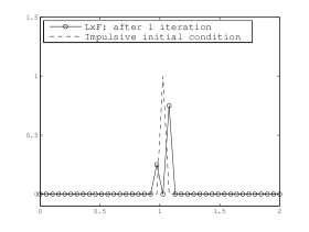
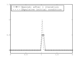
(a)	(b)

Figure 2: Numerical approximation of Linear transport equation (35) with impulsive initial data. (a) By monotone and TVD Lax-Friedrichs scheme: Induced oscillations (b) First order two point upwind scheme: Absence of induced oscillations.

It is interesting to note that two point monotone and TVD upwind scheme does not exhibit induced oscillations in Figure 2(b).

The main aim of this work is to construct uniformly non-oscillatory shock capturing monotone and TVD methods with high accuracy for non-sonic smooth extrema. In order to achieve it, a non-conservative formulation is done using framework of local maximum principle (LMP) with the help of gradient ratio parameter. The rest of paper is organized as: For completeness, in section 3, local maximum principle (LMP) stability is defined for two points schemes. It is shown in Lemma 3.2, that away from sonic point LMP stability implies global monotone and TVD stability. In section 4, we analyze representative uniformly second order schemes in non-sonic region for their TVD (or LMP) stability by converting them into two point schemes. This yields computable bounds for the stability of these scheme and are presented as main results in Theorems 4.1-4.7. These obtained TVD bounds ensure for second rrder TV stable approximation for smooth solution with non-sonic critical point of extreme nature. In section 5, hybrid schemes are designed using the TVD bounds and a shock detector technique. Numerical results are given to support the theoretical results and claim. Conclusion and future work is discussed in section 6.

3 Local maximum principle (LMP) stability

It is clear from the above discussion that the global maximum principle (4) satisfying monotone or TVD stability experience difficulty in the presence of non-monotone data with extrema. These two local phenomena i.e, induced oscillations and degeneracy in accuracy at non-sonic extrema by monotone and TVD schemes motivate us to look for their non-linear stability locally at non-sonic extrema. Consider the following local maximum principle (LMP) for scalar conservation law (1),

$$\min_{x_{i-1}\leq x\leq x_{i}}u(x,t^{n})\leq u(x,t^{n+1})\leq\max_{x_{i-1}\leq x\leq x_{i}}u(x,t^{n}) \;\;\mbox{if}\;f^{{}^{\prime}}(u)>0,$$ (7a)

$$\min_{x_{i}\leq x\leq x_{i+1}}u(x,t^{n})\leq u(x,t^{n+1})\leq\max_{x_{i}\leq x\leq x_{i+1}}u(x,t^{n}) \;\;\mbox{if}\;f^{{}^{\prime}}(u)<0.$$ (7b)

In case of two point schemes, initial solution data will always be monotone as either $u(x_{a},t)\leq u(x_{b},t),\;x_{a}\neq x_{b}$ or vice verse thus the LMP condition (7) reduces to

$$\min(u_{i-1}^{n},u_{i}^{n})\leq u_{i}^{n+1}\leq\max(u_{i-1}^{n},u_{i}^{n}) \;\;\mbox{if}f^{{}^{\prime}}(u)>0,$$ (8a)

$$\min(u_{i}^{n},u_{i+1}^{n})\leq u_{i}^{n+1}\leq\max(u_{i}^{n},u_{i+1}^{n}) \;\;\mbox{if}\;f^{{}^{\prime}}(u)<0.$$ (8b)

Thus away from sonic point $u_{i}^{*}$ i.e., $a_{i+\frac{1}{2}}=f^{{}^{\prime}}(u_{i}^{*})\neq 0$ define,

Definition 3.1.

A numerical scheme is LMP stable (8) if it can be written as

$$u_{i}^{n+1}=\left\{\begin{array}[]{ll}\mathcal{C}u_{i}^{n}+\mathcal{D}u_{i-1}^{n}&\;\;\mbox{if}\;\;\;\;\;\;\;\;\;0<\lambda a^{n}_{i+\frac{1}{2}}\leq 1,\\ \mathcal{C}u_{i}^{n}+\mathcal{D}u_{i+1}^{n}&\;\;\mbox{if}\;\;\;\;\;-1\leq\lambda a^{n}_{i+\frac{1}{2}}<0,\end{array}\right.$$ (9)

where coefficients $\mathcal{C}$and $\mathcal{D}$ are real functions such that $\mathcal{C}\geq 0,\mathcal{D}\geq 0$, $\mathcal{C}+\mathcal{D}=1$.

Scheme (9) is essentially a convex combination of two point values of $u(:,t^{n})$ thus ensures that the updated solution value of $u(x_{i},t^{n+1})$ will remain be bounded by both point values without introducing of new local maxima-minima. Note that two point first order upwind scheme is a natural example of LMP stable scheme with coefficients

$$\mathcal{C}=1-\lambda a_{i-\frac{1}{2}},\mathcal{D}=\lambda a_{i-\frac{1}{2}} \;\;\mbox{if}\;\;\;\;\;0<\lambda f^{{}^{\prime}}(u_{i}^{n})\leq 1$$ (10a)

$$\mathcal{C}=1-\lambda a_{i+\frac{1}{2}},\mathcal{D}=\lambda a_{i+\frac{1}{2}} \;\;\mbox{if}\;\;\;\;\;-1\leq\lambda f^{{}^{\prime}}(u_{i}^{n})<0.$$ (10b)

This justifies the non-occurrence of local oscillation by first order upwind scheme in Figure 2(b). From definition 3.1 it follows,

Lemma 3.2.

Local maximum principle stable scheme (9) is global total variation diminishing stable.

Proof.

Using relation $\mathcal{C}=1-\mathcal{D}$, rewrite (9) in the non-conservative half incremental form as,

$$u_{i}^{n+1}=\left\{\begin{array}[]{ll}u_{i}^{n}-\mathcal{D}(u_{i}^{n}-u_{i-1}^{n})&\;\;\mbox{if}\;\;\;\;\;\;\;\;\;0<\lambda a^{n}_{i+\frac{1}{2}}\leq 1,\\ u_{i}^{n}+\mathcal{D}(u_{i+1}^{n}-u_{i}^{n})&\;\;\mbox{if}\;\;\;\;\;-1\leq\lambda a^{n}_{i+\frac{1}{2}}<0,\end{array}\right.$$ (11)

where from Definition 3.1, $0\leq\mathcal{C}\leq 1$ and $0\leq\mathcal{D}\leq 1$. On appropriately choosing one of the coefficients $\alpha$ or $\beta$ zero in I-form (6), the Lemma 2.2 shows approximation by half I-form (11) is global TVD. ∎

Remark 1.

The LMP stability is defined only in non-sonic region therefore by Lemma 3.2, LMP stability implies TVD stability in non-sonic region i.e., away from sonic point $f^{{}^{\prime}}(u^{*})\neq 0$. In this setting, from next section onward until stated the term LMP/TVD stability implies global TVD stability (5) away from sonic point.

4 Bounds on high order TVD accuracy

In this section using definition 3.1, it is shown that second order total variation diminishing approximation is possible for the solution with non-sonic extreme critical points. It follows from the LMP stability bounds given for the representative second order accurate Lax-Wendroff (LxW), Beam-Warming (BW) and Fromm schemes respectively for scalar problem (1). Let the stencil $[x_{i-s},x_{i+r}]$ of $r+s+1$ point scheme locally does not contain sonic point $u^{*}(x,t)$ i.e., $f^{{}^{\prime}}(u^{*})\neq 0$ and characteristics speed at local cell interfaces is non-zero. Note that the case of degenerate characteristic speed i.e., $a_{i+\frac{1}{2}}=0$ or/and $a_{i-\frac{1}{2}}=0$ are not interesting as these schemes do not necessarily preserve their uniform order of accuracy. We also consider the wave speed slpit $a^{+}_{i+\frac{1}{2}}+a^{-}_{i+\frac{1}{2}}=a_{i+\frac{1}{2}}$ such that $a^{+}_{i+\frac{1}{2}}\geq 0$ and $a^{-}_{i+\frac{1}{2}}\leq 0$. Note that for $a_{i+\frac{1}{2}}>0\Rightarrow a_{i+\frac{1}{2}}=a^{+}_{i+\frac{1}{2}}>0,a^{-}_{i+\frac{1}{2}}=0$ whereas $a_{i+\frac{1}{2}}<0\Rightarrow a_{i+\frac{1}{2}}=a^{-}_{i+\frac{1}{2}}<0,a^{+}_{i+\frac{1}{2}}=0,$. After dropping the superscript for time level $n$, following function definitions and notations are used in the rest of the presentation. Define the smoothness parameter as

$$r^{\pm}_{i}=r^{\pm}(F_{i})=\frac{\left(1\mp\lambda a^{\pm}_{i\mp\frac{1}{2}}\right)\Delta_{\mp}F^{\pm}_{i}}{\left(1\mp\lambda a^{\pm}_{i\pm\frac{1}{2}}\right)\Delta_{\pm}F^{\pm}_{i}},$$ (12)

where the flux split $F^{+}_{i}+F^{-}_{i}=F_{i}$ is consistent with wave split and given by

$$F^{\pm}_{i+1}-F^{\pm}_{i}=a^{\pm}_{i+\frac{1}{2}}(u_{i+1}-u_{i}).$$ (13)

Here the superscript $\pm$ sign of $r_{i}$ denotes the positive/negative sign of wave speed. Also define the signum function

$$\sigma(x)=sgn(x)=\left\{\begin{array}[]{ll}+1&\;if\;x\geq 0,\\ -1&\;if\;x<0.\end{array}\right.$$ (14)

In order to analyze the local non-linear stability of considered schemes we choose practically viable CFL like condition

$$0<\lambda\max_{u}|f^{{}^{\prime}}(u)|<1$$ (15)

Note that the choice $\displaystyle\lambda\max_{u}|f^{{}^{\prime}}(u)|=0\Rightarrow f^{{}^{\prime}}(u)$ corresponds to the case of degenerate characteristic speed or steady state case.

4.1 Centered Lax-Wendroff scheme

Theorem 4.1.

Away from sonic point and under CFL condition (15), the second order accurate Lax-Wendroff scheme for scalar conservation law (1) is TVD in the solution region where

$$r^{\pm}_{i}\in\left(-\infty,\,\kappa_{1}\left(\lambda a^{\pm}_{i\mp\frac{1}{2}}\right)\right)\cup\left(\gamma_{1}\left(\lambda a^{\pm}_{i\mp\frac{1}{2}}\right),\,\infty\right)$$

where numbers $\kappa_{1}<0$, $\gamma_{1}>0$ depends on CFL number for linear stability given by

$$\kappa_{1}(x)=-\frac{1-x\sigma(x)}{1+x\sigma(x))},$$ (16)

$$\gamma_{1}(x)=\frac{x\sigma(x)}{2+x\sigma(x)}.$$ (17)

Proof.

Consider the numerical flux function of Lax-Wendroff (LxW) scheme

$$F^{n,LxW}_{i+\frac{1}{2}}=\frac{1}{2}\left(F_{i+1}+F_{i}\right)-\frac{\lambda\,a^{2}_{i+\frac{1}{2}}}{2}\Delta_{+}{u}_{i}.$$ (18)

In order to ensure non sonic region, let the characteristics speed is locally non-zero. Since LxW uses three point centred stencil $[x_{i-s},x_{i+r}],r=s=1$, it suffice to assume $a_{i+\frac{1}{2}}\times a_{i-\frac{1}{2}}>0.$

• Case $f^{{}^{\prime}}({u})>0$: Let $a_{i\pm\frac{1}{2}}>0$, then the conservative approximation using (18) can be written as

  $${u}^{n+1}_{i}={u}_{i}-\left[\frac{\lambda a_{i+\frac{1}{2}}}{2}\left(1-\lambda\,a_{i+\frac{1}{2}}\right)\Delta_{+}{u}_{i}+\frac{\lambda\,a_{i-\frac{1}{2}}}{2}\left(1+\lambda\,a_{i-\frac{1}{2}}\right)\Delta_{-}{u}_{i}\right],$$ (19)

  which can be written in the following non-conservative half Incremental form (11),

  $${u}^{n+1}_{i}={u}_{i}-\left[\frac{\lambda a_{i+\frac{1}{2}}}{2}\left(1-\lambda\,a_{i+\frac{1}{2}}\right)\frac{\Delta_{+}{u}_{i}}{\Delta_{-}{u}_{i}}+\frac{\lambda\,a_{i-\frac{1}{2}}}{2}\left(1+\lambda\,a_{i-\frac{1}{2}}\right)\right]\Delta_{-}{u}_{i}.$$ (20)

  From Lemma 3.2, half I-from (20) will be TVD if,

  $$0\leq\left[\lambda a_{i+\frac{1}{2}}\left(1-\lambda\,a_{i+\frac{1}{2}}\right)\frac{\Delta_{+}{u}_{i}}{\Delta_{-}{u}_{i}}+\lambda\,a_{i-\frac{1}{2}}\left(1+\lambda\,a_{i-\frac{1}{2}}\right)\right]\leq 2,$$ (21)

  which reduces to,

  $$-\lambda\,a_{i-\frac{1}{2}}\left(1+\lambda\,a_{i-\frac{1}{2}}\right)\leq\lambda\,a_{i+\frac{1}{2}}\left(1-\lambda\,a_{i+\frac{1}{2}}\right)\frac{\Delta_{+}{u}_{i}}{\Delta_{-}{u}_{i}}\leq 2-\lambda\,a_{i-\frac{1}{2}}\left(1+\lambda\,a_{i-\frac{1}{2}}\right)$$ (22)

  Note that $\lambda a_{i-\frac{1}{2}}(1-\lambda\,a_{i-\frac{1}{2}})>0$ under discrete CFL condition,

  $$0<\lambda\,\max_{i}{a_{i+\frac{1}{2}}}<1,$$ (23)

  Hence inequality (22) can be written as

  $$-\frac{(1+\lambda\,a_{i-\frac{1}{2}})}{(1-\lambda\,a_{i-\frac{1}{2}})}\leq\frac{a_{i+\frac{1}{2}}(1-\lambda\,a_{i+\frac{1}{2}})}{a_{i-\frac{1}{2}}(1-\lambda\,a_{i-\frac{1}{2}})}\frac{\Delta_{+}{u}_{i}}{\Delta_{-}{u}_{i}}\leq\frac{2-\lambda a_{i-\frac{1}{2}}(1+\lambda\,a_{i-\frac{1}{2}})}{\lambda\,a_{i-\frac{1}{2}}(1-\lambda\,a_{i-\frac{1}{2}})}$$ (24)

  or

  $$-\frac{(1+\lambda\,a_{i-\frac{1}{2}})}{(1-\lambda\,a_{i-\frac{1}{2}})}\leq\frac{a_{i+\frac{1}{2}}(1-\lambda\,a_{i+\frac{1}{2}})}{a_{i-\frac{1}{2}}(1-\lambda\,a_{i-\frac{1}{2}})}\frac{\Delta_{+}{u}_{i}}{\Delta_{-}{u}_{i}}\leq\frac{2+\lambda\,a_{i-\frac{1}{2}}}{\lambda a_{i-\frac{1}{2}}},$$ (25)

  Using definition (3) and flux wave split (13), Inequality (25) becomes

  $$-\frac{(1+\lambda\,a^{+}_{i-\frac{1}{2}})}{(1-\lambda\,a^{+}_{i-\frac{1}{2}})}\leq\frac{(1-\lambda\,a^{+}_{i+\frac{1}{2}})}{(1-\lambda\,a^{+}_{i-\frac{1}{2}})}\frac{\Delta^{+}_{+}{F^{+}}_{i}}{\Delta^{+}_{-}{F^{+}}_{i}}\leq\frac{2+\lambda\,a^{+}_{i-\frac{1}{2}}}{\lambda a^{+}_{i-\frac{1}{2}}}.$$ (26)

  Inequality (26) on inversion yields,

  $$r^{+}_{i}<\kappa^{+}_{1}(\lambda\,a^{+}_{i-\frac{1}{2}})\;\mbox{OR}\;r^{+}_{i}>\gamma^{+}_{1}(\lambda a^{+}_{i-\frac{1}{2}}),$$ (27)

  where

  $$r^{+}_{i}=\frac{(1-\lambda\,a^{+}_{i-\frac{1}{2}})\Delta^{+}_{-}{F}_{i}}{(1-\lambda\,a^{+}_{i+\frac{1}{2}})\Delta^{+}_{+}{F}_{i}},\;\kappa^{+}_{1}(\lambda a^{+}_{i-\frac{1}{2}})=-\frac{(1-\lambda\,a^{+}_{i-\frac{1}{2}})}{(1+\lambda\,a^{+}_{i-\frac{1}{2}})}\;\mbox{and}\;\displaystyle\gamma^{+}_{1}(\lambda a^{+}_{i-\frac{1}{2}})=\frac{\lambda\,a^{+}_{i-\frac{1}{2}}}{2+\lambda a^{+}_{i-\frac{1}{2}}}.$$

  
  

• Case ${f^{{}^{\prime}}(u)<0}$: Let $a_{i\pm\frac{1}{2}}<0$, then the non-conservative I-form can be written as

  $${u}^{n}_{i}={u}_{i}-\left[\frac{\lambda\,a_{i+\frac{1}{2}}}{2}\left(1-\lambda\,a_{i+\frac{1}{2}}\right)+\frac{\lambda\,a_{i-\frac{1}{2}}}{2}\left(1+\lambda\,a_{i-\frac{1}{2}}\right)\frac{\Delta_{-}{u}_{i}}{\Delta_{+}{u}_{i}}\right]\Delta_{+}{u}_{i}.$$ (28)

  Using Lemma 3.2, half I-from (28) will be TVD if,

  $$0\leq-\frac{\lambda\,a_{i+\frac{1}{2}}}{2}\left(1-\lambda\,a_{i+\frac{1}{2}}\right)-\frac{\lambda\,a_{i-\frac{1}{2}}}{2}\left(1+\lambda\,a_{i-\frac{1}{2}}\right)\frac{\Delta_{-}{u}_{i}}{\Delta_{+}{u}_{i}}\leq 1$$ (29)

  which can be written as

  $$\lambda\,a_{i+\frac{1}{2}}\left(1-\lambda\,a_{i+\frac{1}{2}}\right)\leq-\lambda\,a_{i-\frac{1}{2}}\left(1+\lambda\,a_{i-\frac{1}{2}}\right)\frac{\Delta_{-}{u}_{i}}{\Delta_{+}{u}_{i}}\leq 2+\lambda\,a_{i+\frac{1}{2}}\left(1-\lambda\,a_{i+\frac{1}{2}}\right).$$ (30)

  The discrete CFL condition for $a(u)<0$ is,

  $$-1<\lambda a_{i+\frac{1}{2}}<0,\,\forall i.$$ (31)

  Therefore the quantity $-\lambda a_{i+\frac{1}{2}}(1+\lambda a_{i+\frac{1}{2}})>0.$ Divide Inequality (30) by it and using (3) yields,

  $$-\frac{\left(1-\lambda\,a_{i+\frac{1}{2}}\right)}{\left(1+\lambda a_{i+\frac{1}{2}}\right)}\leq\frac{\left(1+\lambda\,a_{i-\frac{1}{2}}\right)}{\left(1+\lambda a_{i+\frac{1}{2}}\right)}\frac{\Delta_{-}F_{i}}{\Delta_{+}F_{i}}\leq-\frac{2+\lambda\,a_{i+\frac{1}{2}}\left(1-\lambda\,a_{i+\frac{1}{2}}\right)}{\lambda a_{i+\frac{1}{2}}\left(1+\lambda a_{i+\frac{1}{2}}\right)}$$ (32)

  or using flux wave split (13)

  $$-\frac{\left(1-\lambda\,a^{-}_{i+\frac{1}{2}}\right)}{\left(1+\lambda a^{-}_{i+\frac{1}{2}}\right)}\leq\frac{\left(1+\lambda\,a^{-}_{i-\frac{1}{2}}\right)}{\left(1+\lambda a^{-}_{i+\frac{1}{2}}\right)}\frac{\Delta_{-}F^{-}_{i}}{\Delta_{+}F^{-}_{i}}\leq\frac{\lambda\,a^{-}_{i+\frac{1}{2}}-2}{\lambda\;a^{-}_{i+\frac{1}{2}}}$$ (33)

  Inequality (33) on inversion yields,

  $$r^{-}_{i}<\kappa_{1}\left(\lambda a^{-}_{i+\frac{1}{2}}\right)\;\mbox{OR}\;r^{-}_{i}>\gamma_{1}\left(\lambda a^{-}_{i+\frac{1}{2}}\right).$$ (34)

  where $\displaystyle r_{i}^{-}=\frac{\left(1+\lambda a^{-}_{i+\frac{1}{2}}\right)\Delta_{+}F^{-}_{i}}{\left(1+\lambda\,a^{-}_{i-\frac{1}{2}}\right)\Delta_{-}F^{-}_{i}},\;\kappa_{1}\left(\lambda a^{-}_{i+\frac{1}{2}}\right)=\frac{-\left(1+\lambda a^{-}_{i+\frac{1}{2}}\right)}{\left(1-\lambda a^{-}_{i+\frac{1}{2}}\right)}$ and $\displaystyle\gamma_{1}\left(\lambda a^{-}_{i+\frac{1}{2}}\right)=\frac{-\lambda a^{-}_{i+\frac{1}{2}}}{2-\lambda\,a^{-}_{i+\frac{1}{2}}}$.
  Condition (27) and (34) completes the proof.

∎

4.1.1 LxW on Linear problem: Every extrema is non-sonic.

In order to see the improvement in the TVD approximation at non-sonic extrema, consider the linear transport equation

$$\frac{\partial}{\partial t}u(x,t)+a\frac{\partial}{\partial u}(\,u(x,t))=0,\;a\neq 0$$ (35)

In this case the smoothness parameter (12) reduces to $r^{\pm}_{i}=\displaystyle\frac{\Delta_{\mp}u_{i}}{\Delta_{\pm}u_{i}}$. Note that at point of extrema the measure of smoothness is negative i.e, for transport equation (35), every $r^{\pm}_{i}<0$ implies a non-sonic extreme critical point. Following result follows from Theorem 4.1

Corollary 4.2.

Under the linear stability condition $0<\lambda|a|\leq 1$, the second order accurate Lax-Wendroff scheme for (35) is total variation diminishing where $r_{i}\in(\infty,\,\kappa_{1}(a\lambda))\cup(\gamma_{1}(a\lambda),\,\infty)$.

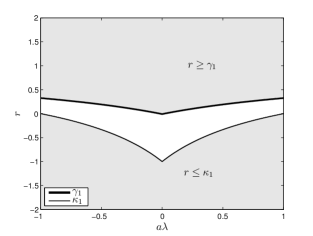
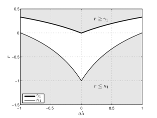
(a)	(b)

Figure 3: (a) : LMP/TVD stability region (shaded) for Lax-Wendroff scheme (b): Zoomed view.

In Figure 3, the behavior of CFL number $a\lambda$ on dependent parameters $\kappa_{1}$ and $\gamma_{1}$ is shown. Note that when $\lambda a\rightarrow 0^{+}$ the parameter $\gamma_{1}\rightarrow 0^{+}$ whilst when $\lambda a\rightarrow 1^{-}$ the parameter $\kappa_{1}\rightarrow 0^{-}$. In particular, for $a|\lambda|=1$, definitions (16), (17) yield non-TVD interval $[\kappa_{1}=0,\gamma_{1}=\frac{1}{3}]$. Note that under linear CFL condition $0<\lambda a\leq 1$, $\kappa_{1}(\lambda\,a)\in(-1,0]$ and $\gamma_{1}(\lambda\,a)\in(0,1/3)$. The following result give CFL independent TVD bounds for LxW scheme [7].

Corollary 4.3.

The Lax-Wendroff scheme for (35) is total variation diminishing under the linear stability condition $0<\lambda|a|\leq 1,$ if $r_{i}=\in(\infty,\,-1)\cup(\frac{1}{3},\,\infty)$

Thus it, can also be concluded from corollary 4.2 and shaded TVD region for LxW scheme in Figure 3 that except for $r_{i}\in[\kappa_{1},\gamma_{1}]$ the second order accurate LxW scheme yields TVD approximation for all solution region including extreme points with $r_{i}<0$. More precisely,

4.2 Upwind Beam-Warming scheme

Theorem 4.4.

Away from sonic point and under CFL condition (15), second order accurate Beam-Warming scheme is TVD for scalar conservation law (1) in the solution region where

$$r^{\pm}_{i\mp 1}\in\left[\kappa_{2}\left(\lambda a^{\pm}_{i\mp\frac{1}{2}}\right),\gamma_{2}\left(\lambda a^{\pm}_{i\mp\frac{1}{2}}\right)\right],$$

where parameter $\gamma_{2}$ and $\kappa_{2}$ defined as,

$$\kappa_{2}(x)=\displaystyle\frac{-(2-x\sigma(x))}{x\sigma(x)}$$ (36)

$$\gamma_{2}(x)=\displaystyle\frac{3-x\sigma(x)}{1-x\sigma(x)}$$ (37)

Proof.

• Case $f^{{}^{\prime}}(u)>0$: In this case, BW stencil use grid points $[x_{i-s},x_{i+r}],s=2,r=0$ thus to ensure locally non-sonic region it suffice to let $a_{i-\frac{k}{2}}>0,k=-1,1,3$. The numerical flux of Beam-Warming scheme is,

  $$F^{n,BW}_{i+\frac{1}{2}}=F_{i}+\frac{a_{i-\frac{1}{2}}}{2}\left(1-\lambda\,a_{i-\frac{1}{2}}\right)\Delta_{-}{u}_{i},\;\;a_{i+\frac{1}{2}}>0.$$ (38)

  Resulting non-conservative half I-form can be written as

  $${u}^{n+1}_{i}={u}_{i}-\left[\frac{\lambda\,a_{i-\frac{1}{2}}}{2}\left(3-\lambda\,a_{i-\frac{1}{2}}\right)-\frac{\lambda\,a_{i-\frac{3}{2}}}{2}\left(1-\lambda\,a_{i-\frac{3}{2}}\right)\frac{\Delta_{-}{u}_{i-1}}{\Delta_{-}{u}_{i}}\right]\Delta_{-}{u}_{i}$$ (39)

  For half I-from (39) to be TVD, from Lemma 3.2

  $$0\leq\frac{\lambda\,a_{i-\frac{1}{2}}}{2}\left(3-\lambda\,a_{i-\frac{1}{2}}\right)-\frac{\lambda\,a_{i-\frac{3}{2}}}{2}\left(1-\lambda\,a_{i-\frac{3}{2}}\right)\frac{\Delta_{-}{u}_{i-1}}{\Delta_{-}{u}_{i}}\leq 1.$$ (40)

  Compound Inequality (40) can be written as,

  $$\lambda a_{i-\frac{1}{2}}(3-\lambda a_{i-\frac{1}{2}})-2\leq\lambda a_{i-\frac{3}{2}}(1-\lambda a_{i-\frac{3}{2}})\frac{\Delta_{-}{u}_{i-1}}{\Delta_{-}{u}_{i}}\leq\lambda a_{i-\frac{1}{2}}(3-\lambda a_{i-\frac{1}{2}})$$ (41)

  Under CFL condition (23), i.e., $0<\lambda a_{i+\frac{1}{2}}<1,\;\forall i$ quantity $\lambda a_{i-\frac{1}{2}}(1-\lambda a_{i-\frac{1}{2}})$ is positive, hence (40) can be written as,

  $$\frac{\lambda a_{i-\frac{1}{2}}(3-\lambda a_{i-\frac{1}{2}})-2}{\lambda a_{i-\frac{1}{2}}(1-\lambda a_{i-\frac{1}{2}})}\leq\frac{a_{i-\frac{3}{2}}(1-\lambda a_{i-\frac{3}{2}})}{a_{i-\frac{1}{2}}(1-\lambda a_{i-\frac{1}{2}})}\frac{\Delta_{-}{u}_{i-1}}{\Delta_{-}{u}_{i}}\leq\frac{(3-\lambda a_{i-\frac{1}{2}})}{(1-\lambda a_{i-\frac{1}{2}})}$$

  or

  $$\frac{\lambda a_{i-\frac{1}{2}}-2}{\lambda a_{i-\frac{1}{2}}}\leq\frac{a_{i-\frac{3}{2}}(1-\lambda a_{i-\frac{3}{2}})}{a_{i-\frac{1}{2}}(1-\lambda a_{i-\frac{1}{2}})}\frac{\Delta_{-}{u}_{i-1}}{\Delta_{-}{u}_{i}}\leq\frac{(3-\lambda a_{i-\frac{1}{2}})}{(1-\lambda a_{i-\frac{1}{2}})}$$

  On using flux wave split (13) we get

  $$\frac{\lambda a^{+}_{i-\frac{1}{2}}-2}{\lambda a^{+}_{i-\frac{1}{2}}}\leq\frac{(1-\lambda a_{i-\frac{3}{2}})}{(1-\lambda a_{i-\frac{1}{2}})}\frac{\Delta_{-}F^{+}_{i-1}}{\Delta_{-}F^{+}_{i}}\leq\frac{(3-\lambda a^{+}_{i-\frac{1}{2}})}{(1-\lambda a^{+}_{i-\frac{1}{2}})}$$

  Which, using (12) can be written as,

  $$\kappa_{2}\left(\lambda\,a^{+}_{i-\frac{1}{2}}\right)\leq r^{+}_{i-1}\leq\gamma_{2}\left(\lambda\,a^{+}_{i-\frac{1}{2}}\right)$$ (42)

  where $\kappa_{2}$ and $\gamma_{2}$ are defined in (36) and (37).
  

• Case $f^{{}^{\prime}}(u)<0$: In case of negative characteristics speed, BW use stencil $[x_{i-s},x_{i+r}],s=0,r=2]$ thus to ensure locally non-sonic region it suffice to let $a_{i+\frac{k}{2}}>0,k=-1,1,3$. In case of negative wave speed the Beam-Warming flux is given by,

  $$F^{n,BW}_{i+\frac{1}{2}}=F_{i+1}-\frac{a_{i+\frac{3}{2}}}{2}\left(1+\lambda\,a_{i+\frac{3}{2}}\right)\Delta_{+}{u}_{i+1},\;\;a_{i+\frac{1}{2}}>0.$$ (43)

  Resulting non-conservative half I-form is,

  $${u}^{n+1}_{i}={u}_{i}+\left[\frac{\lambda\,a_{i+\frac{3}{2}}}{2}\left(1+\lambda\,a_{i+\frac{3}{2}}\right)\frac{\Delta_{+}{u}_{i+1}}{\Delta_{+}{u}_{i}}-\frac{\lambda\,a_{i+\frac{1}{2}}}{2}\left(3+\lambda\,a_{i+\frac{1}{2}}\right)\right]\Delta_{+}{u}_{i}.$$ (44)

  Condition for (44) to be TVD is

  $$0\leq\lambda\,a_{i+\frac{3}{2}}\left(1+\lambda\,a_{i+\frac{3}{2}}\right)\frac{\Delta_{+}{u}_{i+1}}{\Delta_{+}{u}_{i}}-\lambda\,a_{i+\frac{1}{2}}\left(3+\lambda\,a_{i+\frac{1}{2}}\right)\leq 2$$ (45)

  $$\lambda\,a_{i+\frac{1}{2}}\left(3+\lambda\,a_{i+\frac{1}{2}}\right)\leq\lambda\,a_{i+\frac{3}{2}}\left(1+\lambda\,a_{i+\frac{3}{2}}\right)\frac{\Delta_{+}{u}_{i+1}}{\Delta_{+}{u}_{i}}\leq 2+\lambda\,a_{i+\frac{1}{2}}\left(3+\lambda\,a_{i+\frac{1}{2}}\right)$$ (46)

  Note under CFL condition (31) $-1\leq\lambda\,a_{i+\frac{1}{2}}<0,\,\forall i$, $\lambda\,a_{i+\frac{1}{2}}\left(1+\lambda\,a_{i+\frac{1}{2}}\right)$ is negative. Compound Inequality (46) reduced to

  $$\frac{2+\lambda\,a_{i+\frac{1}{2}}\left(3+\lambda\,a_{i+\frac{1}{2}}\right)}{\lambda\,a_{i+\frac{1}{2}}\left(1+\lambda\,a_{i+\frac{1}{2}}\right)}\leq\frac{a_{i+\frac{3}{2}}\left(1+\lambda\,a_{i+\frac{3}{2}}\right)}{a_{i+\frac{1}{2}}\left(1+\lambda\,a_{i+\frac{1}{2}}\right)}\frac{\Delta_{+}{u}_{i+1}}{\Delta_{+}{u}_{i}}\leq\frac{\left(3+\lambda\,a_{i+\frac{1}{2}}\right)}{\left(1+\lambda\,a_{i+\frac{1}{2}}\right)}$$ (47)

  or

  $$\frac{\lambda\,a_{i+\frac{1}{2}}+2}{\lambda\,a_{i+\frac{1}{2}}}\leq\frac{a_{i+\frac{3}{2}}\left(1+\lambda\,a_{i+\frac{3}{2}}\right)}{a_{i+\frac{1}{2}}\left(1+\lambda\,a_{i+\frac{1}{2}}\right)}\frac{\Delta_{+}{u}_{i+1}}{\Delta_{+}{u}_{i}}\leq\frac{\left(3+\lambda\,a_{i+\frac{1}{2}}\right)}{\left(1+\lambda\,a_{i+\frac{1}{2}}\right)}$$ (48)

  on using (13)

  $$\frac{\lambda\,a^{-}_{i+\frac{1}{2}}+2}{\lambda\,a^{-}_{i+\frac{1}{2}}}\leq\frac{\left(1+\lambda\,a^{-}_{i+\frac{3}{2}}\right)}{\left(1+\lambda\,a_{i+\frac{1}{2}}\right)}\frac{\Delta_{+}F^{-}_{i+1}}{\Delta_{+}F^{-}_{i}}\leq\frac{\left(3+\lambda\,a^{-}_{i+\frac{1}{2}}\right)}{\left(1+\lambda\,a^{-}_{i+\frac{1}{2}}\right)}$$ (49)

  Using (12), (36) and (37) Inequality (49) can be written as,

  $$\kappa_{2}\left(\lambda\,a^{-}_{i+\frac{1}{2}}\right)\leq r^{-}_{i+1}\leq\gamma_{2}\left(\lambda\,a^{-}_{i+\frac{1}{2}}\right)$$ (50)

∎

4.2.1 BW on Linear problem

Corollary 4.5.

Beam-Warming scheme for (35) is total variation diminishing under the linear stability condition $0<\lambda|a|\leq 1$, if the smoothness parameter $r^{\pm}_{i\mp 1}\in[\kappa_{2}(\lambda a),\gamma_{2}(\lambda a)]$

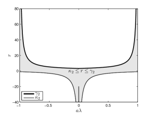
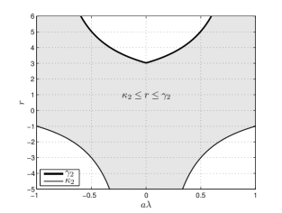
(a)	(b)

Figure 4: (a) : LMP/TVD stability region (shaded) for Beam-Warming scheme (b): Zoomed view.

In Figure 4, TVD region for Beam-Warming scheme is shown as shaded region. It can be deduced that

1. $\lambda a\rightarrow 0^{+}$ Beam-Warming scheme yield TVD approximation for $r_{i-\sigma(a)}\in(-\infty,3]$.

2. $\lambda a\rightarrow 1^{-}$ Beam-Warming scheme yield TVD approximation for $r_{i-\sigma(a)}\in[-1,\infty)$.

Note that for $\lambda|a|\in(0,1]$ parameters $\kappa_{2}\in(-\infty,-1]$ and $\gamma_{2}\in[3,\infty)$. Following CFL number independent weaker TVD bounds can be concluded

Corollary 4.6.

The Beam-Warming scheme for (35) is total variation diminishing under the linear stability condition $0<\lambda|a|<1,$ if $r^{\pm}_{i\mp 1}=[-1,3]$.

4.3 Fromm’s scheme

A less ocsillatory and second order accurate scheme is obtained by using a simple average of LxW and BW flux i.e.,

$$F^{n,FROMM}_{i+\frac{1}{2}}=\frac{1}{2}\left(F^{n,LxW}_{i+\frac{1}{2}}+F^{n,BW}_{i+\frac{1}{2}}\right)$$ (51)

From Theorem 4.1 and Theorem 4.4 following result can be proved,

Theorem 4.7.

Away from sonic point and CFL condition (15), the Fromm’s scheme corresponding to flux (51) for scalar conservation law (1) is TVD in the solution region where

$$r^{\pm}_{i}\in\left(-\infty,\,\kappa_{1}\left(\lambda a^{\pm}_{i\mp\frac{1}{2}}\right)\right)\cup\left(\gamma_{1}\left(\lambda a^{\pm}_{i\mp\frac{1}{2}}\right),\,\infty\right)$$

and

$$r^{\pm}_{i\mp 1}\in\left[\kappa_{2}\left(\lambda a^{\pm}_{i\mp\frac{1}{2}}\right),\gamma_{2}\left(\lambda a^{\pm}_{i\mp\frac{1}{2}}\right)\right].$$

where parameter $\kappa_{1},\gamma_{1},\kappa_{2}$ and $\gamma_{2}$ are defined in (16), (17), (36) and (37) respectively.

5 Hybrid high order LMP/TVD stable schemes

It follows from the Theorem 4.1, 4.4 and Theorem 4.7 that it is possible to achieve second or higher order TVD approximation for most solution region including non-sonic exterma where $r_{i}<0$. In order to demonstrate it numerically, we construct hybrid schemes using a monotone/TVD scheme as complementary conservative scheme (CCS). The following hybrid schemes are the natural choice which satisfies the LMP/TVD bounds obtained in previous section and thus ensures a LMP/TVD approximation. The second order accurate LMP/TVD schemes use second order LxW and BW schemes in the region of their LMP/TVD stability using bounds on smoothness parameter in Theorem 4.1 and 4.4 respectively, otherwise use a conservative conservative scheme (CCS).

5.1 Centered scheme: LW-CCS

1:  if $r^{\pm}_{i}\leq\kappa_{1}$ OR $r^{\pm}_{i}\geq\gamma_{1}$ then

2:     Update $u_{i}^{n+1}\leftarrow$ LxW scheme

3:  else

4:     Update $u_{i}^{n+1}\leftarrow$ CCS.

5:  end if

5.2 Upwind Scheme: BW-CCS

1:  if ($r^{\pm}_{i\mp 1}\geq\kappa_{2}$ AND $r^{\pm}_{i\mp 1}\leq\gamma_{2}$) then

2:     Update $u_{i}^{n+1}\leftarrow$ BW scheme

3:  else

4:     Update $u_{i}^{n+1}\leftarrow$ CCS.

5:  end if

5.3 Centred-Upwind scheme: FLWBW-CCS approximation

This LMP/TVD stable scheme can be obtained using Fromm scheme in its region of LMP/TVD stability using bounds in 4.7 along with schemes 5.1 and 5.2 as follows

1:  if ($r^{\pm}_{i}\leq\kappa_{1}$ OR $r^{\pm}_{i}\geq\gamma_{1}$) AND ($r^{\pm}_{i\mp 1}\geq\kappa_{2}$ AND $r^{\pm}_{i\mp 1}\leq\gamma_{2}$) then

2:     Update $u_{i}^{n+1}\leftarrow$ Fromm’s scheme

3:  else if $r^{\pm}_{i}\leq\kappa_{1}$ OR $r^{\pm}_{i}\geq\gamma_{1}$ then

4:     Update $u_{i}^{n+1}\leftarrow$ LxW scheme

5:  else if ($r^{\pm}_{i\mp 1}\geq\kappa_{2}$ AND $r^{\pm}_{i\mp 1}\leq\gamma_{2}$) then

6:     Update $u_{i}^{n+1}\leftarrow$ BW scheme

7:  else

8:     Update $u_{i}^{n+1}\leftarrow$ CCS.

9:  end if

Note that the scheme 5.1-5.3 are non-conservative as they are based on TVD conditions on the smoothness parameter dedced from the non-conservative form of studied schemes. Therefore they capture the steady shock accurately but may produce moving shock at wrong location see results in Figure 9(a). Note that incorrect shock location by scheme 5.1 is legging whereas by scheme 5.2 it is leading to the exact shock location in Figure 9(a). It is interesting to see the scheme 5.3 cancels the leading and legging errors and gives exact shock location in Figure 10(a). This phenomena of yielding wrong moving shock location by non-conservative schemes along with the shock correction criteria is well explained in [14]. The idea for shock correction is to apply locally a shock capturing conservative scheme in the vicinity of discontinuity using a shock detector. It is therefore, to capture the moving shock correctly, the following hybrid approach can be used,

5.4 Shock Correction: SC-LW-CCS, SC-BW-CCS, SC-FLWBW-CCS hybrid schemes

1:  if Shock region then

2:     Update $u_{i}^{n+1}\leftarrow$ use CCS,

3:  else

4:     Update $u_{i}^{n+1}\leftarrow$ with either of algorithm 5.1-5.3.

5:  end if

5.5 Extension to system of hyperbolic conservation laws

Consider the hyperbolic systems of conservation law in one dimensions,

$$\frac{\partial}{\partial t}\textbf{u}+\frac{\partial}{\partial x}\textbf{F(u)}=0,$$ (52)

where u is vector of conserved quantities $u^{j},\,i=1,2,\dots l$ and F is the vector flux function. The above proposed schemes for scalar case are extended to non-linear systems (52) in the natural manner using flux vector splitting and average flux Jacobian matrix $A=\textbf{F}^{{}^{\prime}}\textbf{(u)}$ of the flux function. In particular for the numerical results presented in next section, the Steger-Warming flux vector splitting is used for 1D and 2D systems. The average Jacobian matrix is computed as follows,

$$A^{n}_{i+\frac{1}{2}}=A\left(\frac{\textbf{u}^{n}_{i+1}+\textbf{u}^{n}_{i}}{2}\right).$$

In order to compute the TVD bounds, the $n-$characteristic speeds associated with system 52)

$$a^{j}_{i+\frac{1}{2}}=\left\{\begin{array}[]{cc}\frac{F^{j}_{i+1}-F^{j}_{i}}{u^{j}_{i+1}-u^{j}_{i}}&{u^{j}_{i+1}-u^{j}_{i}}\neq 0\\ \sigma(A_{i+\frac{1}{2}})&else,\end{array}\right.j=1,2\dots l,$$ (53)

where $\sigma_{i+\frac{1}{2}}$ is the spectrum of eigen values of $A_{i+\frac{1}{2}}$. In above computation (53) the nonphysical discrete wave speed caused by numerical overflow in case of $u^{j}_{i+1}\approx u^{j}_{i}$ are corrected using following way which is similar to the wave speed correction technique proposed in [15]. It is done as,

$$a^{j}_{i+\frac{1}{2}}=\sigma_{max}\;\mbox{if}\;|a^{j}_{i+\frac{1}{2}}|\geq\sigma_{max},$$ (54)

$$a^{j}_{i+\frac{1}{2}}=\sigma_{min}\;\mbox{if}\;|a^{j}_{i+\frac{1}{2}}|\leq\sigma_{min},$$ (55)

where $\sigma_{max}$ and $\sigma_{min}$ refer to the local maxima and minima of the magnitudes of characteristic speeds associated with system (52). For example, the one dimensional Euler equations has the eigenvalues $u,\;u\pm c$ where $u$ and $c$ denotes fluid velocity and the speed of sound respectively. In this case, we define

$$\,\sigma_{\max} = \max{(\max{(|u|,|u-c|,|u+c|)_{i}},\max{(|u|,|u-c|,|u+c|)_{i+1})}},$$ (56)

$$\sigma_{\min} = \max{(\min{(|u|,|u-c|,|u+c|)_{i}},\min{(|u|,|u-c|,|u+c|)_{i+1})}}.$$ (57)

5.6 Shock Sensor

In order to locate the presence of discontinuities, a shock detector proposed in [27] with some modification is used. A brief detail on the shock switch is given below for the sake of completeness of the discussion on numerical implementation.

• Check multigrid ratio check

  $$MR(i,h)=\frac{T_{C}(i,h)}{T_{F}(i,h)+\epsilon}$$

  where $T_{C}(i,2h)$ and $T_{F}(i,h)$ are the $(4^{th},5^{th}\;\mbox{and}\;6^{th})$ order truncation error sum on a coarse (with N/2 grid points) and fine grid (with N points) respectively. The derivatives in this step are calculated by by sixth order compact scheme proposed in [23]. The small parameter $0<\epsilon<<1$ is used to avoid division by zero.

• Calculate the local ratio check at the grid point $x_{i}$ which has multigrid ratio $MR(i,h)\leq 4$,

  $$LR(i)=\left|\frac{\left(u^{{}^{\prime}}_{R}\right)^{2}-\left(u^{{}^{\prime}}_{L}\right)^{2}}{\left(u^{{}^{\prime}}_{R}\right)^{2}+\left(u^{{}^{\prime}}_{R}\right)^{2}+\epsilon}\right|$$

  where $u^{{}^{\prime}}_{L}=3u_{i}-4u_{i-1}+u_{i-2}$ and $u^{{}^{\prime}}_{R}=3u_{i}-4u_{i+1}+u_{i+2}$ left and right slope respectively at grid point $x_{i}$.

• Use a cutoff value $\delta\in(0,1]$ to create a shock switch (SS) on the result of step 2. i.e.,

  $$SS(i)=\left\{\begin{array}[]{ll}0,&\mbox{if}\;LR(i)<\delta\;\mbox{i.e., data is locally smooth around grid point}\;x_{i},\\ 1,&\mbox{if}\;LR(i)\geq\delta\;\mbox{i.e., data is discontinuous around grid point}\;x_{i}.\end{array}\right.$$

Note that the above shock detector has parameters $\epsilon$ and $\delta$ which governs the sensitivity of shock switch. It is observed in numerical computations that for larger value of parameters e.g., $\epsilon=1\times 10^{-2},\delta=0.8$ above shock switch is less sensitive for mild shock or sharp turns and detects only strong shocks whereas $\epsilon=1\times 10^{-8},\delta=0.2$ detect corners and mild shock along with the strong shock. Also in case of non-linear systems, it is observed that small oscillations may arise in the vicinity of shock depending on the choice of shock parameters $\epsilon,\delta$. It is therefore, to make it robust and less prone to parameters $\epsilon,\delta$ a slight modification is done as follows,

• Treat neighbouring grid point $x_{i\pm 1}$ in discontinuity region if $SS(i)=1$ i.e., use $SS(i\pm 1)=1$ if $SS(i)=1$.

6 Numerical Results

In this section numerical results are presented for various benchmark scalar and system test problems in both one and two dimensions. Different smooth as well discontinuous initial conditions are taken to show the performance of schemes in section 5 in terms of accuracy and discontinuity capturing respectively. Numerical results show that the proposed hybrid scheme, due to improved accuracy at extrema and steep gradient region, nicely approximates the smooth region of solution with crisp resolution for rarefaction, contact and shock discontinuities. Moreover it produces the total variation diminishing numerical approximation.

6.1 Linear transport equation: every extrema is non-sonic

Consider the linear transport equation

$$u_{t}+u_{x}=0,\;u(x,0)=u_{0}(x)$$ (58)

with periodic boundary condition. The exact solution of (58) equation convects with out changing the initial shape of $u_{0}(x)$ and is given by $u(x,t)=u_{0}(x-t)$. Note that in general number of extrema are finite and clipping error due to degenerate accuracy at smooth extrema by existing high order monotone and TVD method is visible only after a long period of time in form of approximation of smooth extrema with corners or flatten profile see Figure 5(a). Also due to degenerate accuracy at extrema and steep gradient region their erratic convergence rate can be seen only after a long time see Table 3. It is therefore, probably the transport equation (58) the only test which can be used to check the large time performance of any method. Since the problem (58) is linear thus discontinuities present in the solution does not represents shock or rarefaction therefore scheme 5.3 can be directly applied for this test problem with out shock switch. The numerical computation for problem (58) is done by using the first order upwind scheme as complementary conservative scheme (CCS) in hybrid scheme 5.3 and results are shown by legend method.

6.1.1 Accuracy check: smooth initial condition

Consider 58) along with the the following three different initial conditions which comprises of smooth extrema, monotone region with mild as well sharp turn.

1. Smooth extrema

   $$u(x,0)=\sin(\pi x),\;x\in[-1,\;1].$$ (59)

   The initial profile consists smooth extreme points at $x=\pm\frac{1}{2}$ which preservingly convects to the right direction.

2. Smooth extrema with monotone data region

   $$u(x,0)=\sin^{4}(\pi x),\;x\in[0,\;1].$$ (60)

   This initial condition is taken from [47] and has a smooth extrema at $x=0.5$ with monotone solution regions with mild turn towards the bottom.

3. Smooth extrema with steep gradient region

   $$u(x,0)=\left\{\begin{array}[]{ll}e^{\frac{-1}{1-x^{2}}}&x\in[-1:1]\\ 0&else\end{array}\right.$$ (61)

   This initial condition has a smooth extrema at $x=0$. Compared to initial condition (60) it has high gradient monotone region with sharp turns towards the bottom where $r\rightarrow 0+$ or $r>>1$ respectively. This is a good test to see the degenerate convergence rate for any limiter based TVD scheme.

For smooth initial data numerical solution plots are given at large time level $\bf T_{s}$. The convergence rate of scheme 5.4 is given at various time instance with varying $CFL$ number to show the robust and higher than second order convergence rate of the method 5.3. In Figure 5(a), numerical solution obtained by method corresponding to IC (59) is compared with high order TVD Lax-Wendroff flux limited method (LxWFLM) [31] with compressive Superbee limiter [32]. In Figure 6 and Figure 7 approximate solution is given for transport problem corresponding to initial conditions (60) and (61) respectively. The total variation of the computed solution obtained by method is compared with uniformly second order LxW, BW and Fromm schemes respectively for all three IC’s in Figure 5(b), 6(b) and 7(c).

From the numerical results in it is evident that problem of flattening of smooth round shaped solution profile is removed due to improved approximation of extreme points. Moreover it can be observed and Figure 6(a) that this improvement more visible as $\lambda a\rightarrow 1$ which support the improved TVD region for extrema of LxW as discussed in the Corollary 4.2. Total variation plots show that total variation for designed scheme 5.3 is decreasing whilst uniformly second order LxW and BW schemes do not produce TVD solution though it remain total variation bounded (TVB).

In Table 1, discrete maximum $L^{\infty}$ error convergence rate is given for scheme 5.3 as $L^{\infty}$ error is the best indicator for checking the performance of any scheme in terms of clipping error due to drop in accuracy at smooth extrema. In Table 2 and Table 4, error convergence rates are given in terms of $L^{1}$ and $L^{\infty}$ error for method with different choice of $CFL$ and time for linear test corresponding to initial conditions (60) and (61) respectively. The numerical results show that the designed scheme 5.3 shows higher than second order convergence rate independently of the choice of $CFL$ number or final time $T$. Also due to improved approximation of extrema and steep gradient region, the used method yields smooth approximation with out clipping error which support the Corollary 4.2 and 4.3.

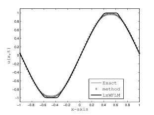
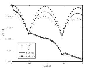
(a) at $T=30$.	(b) at $T=2$ with $CFL=0.95$.

Figure 5: Solution of (58) with IC (59) using $N=80$: (a) Flatten approximation for smooth extrema by LxWFLM whereas proposed scheme 5.4 preserve solution with smooth extrema with out introducing corners. (b) Comparison of total variation.

T=2	T=30
CFL=0.5 CFL=0.95 N $L^{\infty}$ error Rate 20 9.1927e-03 … 40 1.9456e-03 2.240 80 3.7656e-04 2.369 160 7.0744e-05 2.412 320 1.2599e-05 2.489 640 3.2485e-06 1.955 $L^{\infty}$ error Rate 1.4026e-03 … 2.6640e-04 2.396 5.6365e-05 2.241 1.1332e-05 2.314 2.6879e-06 2.076 3.1057e-07 3.113	CFL=0.5 CFL=0.95 $L^{\infty}$ error Rate 6.3628e-02 … 1.0892e-02 2.546 1.8543e-03 2.554 3.3400e-04 2.473 4.1812e-05 2.998 3.5142e-06 3.573 $L^{\infty}$ error Rate 1.1716e-02 … 2.2095e-03 2.407 4.4726e-04 2.305 8.6187e-05 2.376 1.4613e-05 2.560 4.5598e-07 5.002

Table 1: Consistent higher than second order $L^{\infty}$ convergence rate with the mesh refinement corresponding to initial condition (59).

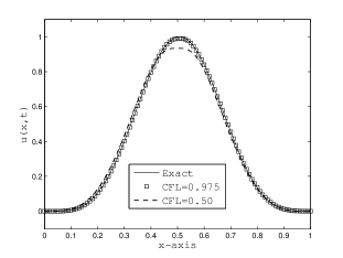
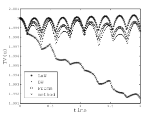
(a)	(b)

Figure 6: Solution for linear equation (35) with IC (60) (a) at time $T=20,\;N=100$, Smooth approximation of extrema with reduced clipping error: (b) TV plot up to $T=2$ using $N=80,CFL=0.95$.

CFL=0.5	CFL=0.95
N $L^{1}$ Error Rate $L^{\infty}$ error Rate 40 7.6962e-02 … 6.1348e-03 … 80 1.7350e-02 2.149 1.1039e-03 2.474 160 3.8066e-03 2.188 1.9596e-04 2.494 320 7.3723e-04 2.368 2.4368e-05 3.008 640 1.1693e-04 2.656 4.3613e-07 5.804 1280 2.8601e-05 2.031 5.4189e-08 3.009 2560 7.0685e-06 2.017 6.6891e-09 3.018	$L^{1}$ Error Rate $L^{\infty}$ error Rate 1.3179e-02 … 1.4315e-03 … 3.4723e-03 1.924 2.7228e-04 2.394 8.7436e-04 1.990 5.2159e-05 2.384 2.0210e-04 2.113 8.6669e-06 2.589 3.2508e-05 2.636 1.1141e-07 6.282 8.0887e-06 2.007 1.3877e-08 3.005 2.0182e-06 2.003 1.7315e-09 3.003

Table 2: Order of convergence with the mesh refinement at $T=20$ corresponding to initial condition (60).

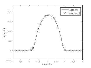
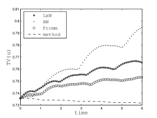
(a)	(b)

Figure 7: Solution for linear equation (35) with IC (61) at time $T=6$ and $N=100,\;CFL=0.95$. (a) Smooth approximation of extrema with no clipping error by Scheme 5.1. (b) Comparison of total variation.

I-Order Upwind	Second order TVD scheme
N $L^{1}$ Error Rate $L^{\infty}$ error Rate 80 2.5248e-01 0.583 1.6091e-02 1.482 160 1.6210e-01 0.639 5.8392e-03 1.462 320 9.7673e-02 0.731 2.2646e-03 1.367 640 5.6346e-02 0.794 8.2206e-04 1.462 1280 3.1355e-02 0.846 2.8328e-04 1.537 2560 1.6889e-02 0.893 9.2241e-05 1.619	$L^{1}$ Error Rate $L^{\infty}$ error Rate 2.2319e-02 1.314 2.4725e-03 2.294 1.6468e-02 0.439 1.3464e-03 0.877 5.2704e-03 1.644 2.0531e-04 2.713 2.3125e-03 1.188 8.7812e-05 1.225 1.0757e-03 1.104 4.1735e-05 1.073 4.1654e-04 1.369 1.0950e-05 1.930

Table 3: Order of convergence using I order upwind and LxW flux limited TVD method with Superbee limiter at $T=6,CFL=0.5$ corresponding to initial condition (61).

CFL=0.5	CFL=0.95
N $L^{1}$ Error Rate $L^{\infty}$ error Rate 80 4.3378e-02 1.654 4.9870e-03 2.139 160 1.2992e-02 1.739 1.3187e-03 1.919 320 3.2156e-03 2.014 2.6333e-04 2.324 640 6.1867e-04 2.378 3.8218e-05 2.785 1280 1.1353e-04 2.446 4.1315e-06 3.210 2560 1.7115e-05 2.730 3.6114e-07 3.516	$L^{1}$ Error Rate $L^{\infty}$ error Rate 1.1681e-02 1.646 2.2055e-03 2.239 3.2801e-03 1.832 5.0305e-04 2.132 8.1011e-04 2.018 8.1325e-05 2.629 1.7801e-04 2.186 1.3173e-05 2.626 4.5829e-05 1.958 1.8927e-06 2.799 1.2376e-05 1.889 2.5213e-07 2.908

Table 4: Consistent higher than second order of convergence with the mesh refinement at $T=6$ corresponding to initial condition (61)

6.1.2 Discontinuous initial condition

In this test is taken from [6] originally used by Harten in [12]. Initial solution is complex in nature which contains parts of smooth solution, mix discontinuities, discontinuities of derivative in the interval $[-1,1]$. In Figure 8(a), numerical results is given by proposed method and in Figure 8(b) the total variation plot of the computed solution by method is given.

$$u_{0}(x)=\left\{\begin{array}[]{lcl}2x+2-sin(3\pi(x-0.5))/6&\mbox{if}&-1\leq x\leq 0.5,\\ (0.5-x)sin(1.5\pi(x-0.5)^{2})&\mbox{if}&-0.5<x<1/6,\\ |sin(2\pi(x-0.5))|&\mbox{if}&1/6<x<=5/6,\\ 2x-2-sin(3\pi(x-0.5))/6&\mbox{if}&5/6<x<=1.\\ \end{array}\right.\\$$ (62)

It can be seen in Figure 8 that the proposed scheme 5.3 yields TVD solution with crisp capturing of the discontinuities with out clipping error at smooth extrema. The error convergence rate is not shown for this discontinuous test problem as discontinuities can only be approximated with at most first order of accuracy [36]

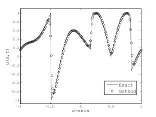
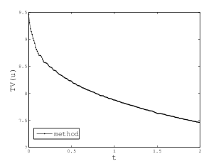
(a)	(b)

Figure 8: (a) High resolution oscillation free solution for test problem 62 by scheme 5.4 for data $CFL=0.95,\,N=160,\,T=2.0$. (b) Total variation decreasing plot of method

6.2 Non-linear case: Burgers equation

Consider the Burgers equation

$$u_{t}+\left(\frac{u^{2}}{2}\right)_{x}=0,-a\leq x\leq b$$ (63)

with initial condition $u_{0}(x)$ and periodic boundary conditions. It is the non-linear nature of the equation (63) that even for smooth initial condition, the solution of (63) eventually develops discontinuities like rarefaction and shocks after breaking time $T_{b}$ given by

$$T_{b}=\frac{-1}{\min_{x}(u^{{}^{\prime}}_{0}(x))}$$ (64)

Also the unique sonic point for Burgers equation (63) is $u^{*}=0$. It is therefore, Burgers equation is a good test to check the performance of any scheme for smooth as well discontinuous solutions profile at pre and post-shock time $T_{b}$ respectively. In the numerical computation FORCE scheme is used as CCS in schemes 5.1 to 5.3 and their respective hybrid shock corrected analog in scheme 5.4.

6.2.1 Shock correction moving shock

We first consider the following discontinuous initial condition to show the non-conservative nature of schemes 5.1, 5.2 and 5.3 as they yield solution with wrong location of moving shock.

$$u(x,0)=\left\{\begin{array}[]{cc}1,&|x|\leq\frac{1}{3},\\ 0,&else.\end{array}\right.$$ (65)

The solution corresponding to IC (65), develops a rarefaction wave and a moving shock which corresponds to initial discontinuities at $x=-1/3$ and $x=1/3$ respectively. In Figure 9(a) results obtained by second order Lax-Wendroff (LW-FORCE) and Beam-Warming (BW-FORCE) schemes 5.1 and 5.2 respectively are given. It is clear that shock location given by LW-FORCE is legging behind whereas by BW-FORCE it is leading ahead of exact shock location. Results by shock corrected schemes SC-LW-FORCE and SC-BW-FORCE as described in 5.4 are given in 9(b) which show correct location of shock is recovered with out loosing crisp resolution of left rarefaction. Numerical results in Figure 10(a), obtained by scheme 5.3 (FLWBW-FORCE) shows that shock is crisply captured at right location with high resolution for bottom and top of left rarefaction. In Figure 10(b), results by SC-FLWBW-FORCE are given which show little dissipative resolution for shock which is due to approximation by dissipative FORCE scheme in the vicinity of shock.

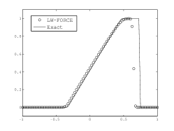
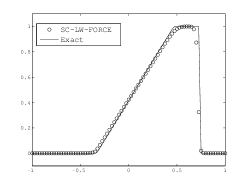
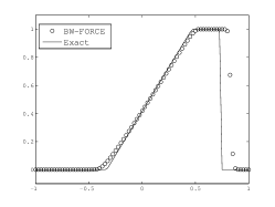
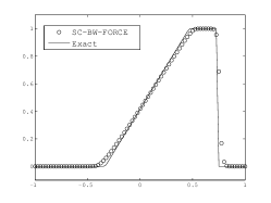
(a)	(b)

Figure 9: Solution at $T=0.8$ using $CFL=0.8,\;N=80$, (a) Wrong location of moving shock using Scheme 5.1 and 5.2 (b) Shock correction using shock switch.

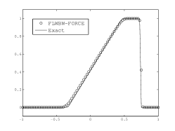
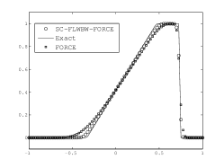
(a)	(b)

Figure 10: Solution at $T=0.8$ using $CFL=0.8,\;N=80$, (a) Scheme 5.3 give correct shock location high resolution for left rarefaction and crisp capturing for the moving shock, (b) Solution by Scheme 5.4.

6.2.2 Accuracy Check: Smooth Initial conditions

Consider three different smooth initial conditions (IC) along with corresponding breaking time $T_{b}$

$$u(x,0)=0.1+sin^{4}(\pi x),\,x\in[0,\,1],\;T_{b}=0.27803225$$ (66)

$$u(x,0)=0.1+\exp^{-x^{4}},\,x\in[-2:3],\;T_{b}=0.65669683.$$ (67)

$$u(x,0)=\frac{1}{4}(1+sin(\pi x)),\,x\in[-1:1],\;T_{b}=\frac{4}{\pi}.$$ (68)

IC (66) and (67) does not contain any sonic point whereas IC (68) has a sonic point at $x=-0.5$ since $u(-0.5,0)=0$. The solution corresponding to IC (66) and (67) develop a moving shock followed by a rarefaction fan whereas the moving shock corresponding to IC (68) is separated by two rarefaction fans. In Figure 11, 12 and 13 the pre and post-shock solution of Burgers equation obtained by the shock corrected hybrid Scheme 5.4 (SC-FLWBW-FORCE) corresponding to IC (66), (67) and (68) respectively are given. The total variation plots are also given for different choices of CFL number $\lambda\max_{u}|f^{{}^{\prime}}(u)|$. In Table 5 to Table 7, $L^{1}$ and $L^{\infty}$ errors are shown at pre-shock time $\displaystyle T_{b}$ using different CFL number. Results show that the hybrid scheme nicely approximated pre-shock solution with out clipping error and does not introduce induced oscillations near shock in the post-shock solution. Moreover purposed method yields a total variation diminishing solution and shows a consistent convergence rate between second and third order in both the norms.

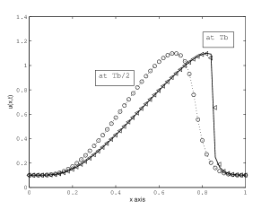
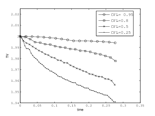
(a)	(b)

Figure 11: Burgers equation solution using SC-FLWBW-FORCE corresponding to IC (66): (a) No clipping error for smooth extrema as well near shock zone $CFL=0.95,N=50$, (b) Effect of CFL on total variation of computed solution

N	CFL=0.6	CFL=0.9
10 20 40 80 160 320 640	$L^{1}$ error Rate $L^{\infty}$ error Rate 3.1074e-02 … 1.2720e-02 … 1.3874e-02 1.1634 4.6798e-03 1.4426 2.0530e-03 2.7566 3.9157e-04 3.5791e 4.0690e-04 2.3350 6.9600e-05 2.4921e 8.6630e-05 2.2317 1.2510e-05 2.4760e 1.4700e-05 2.5591 1.2000e-06 3.3820e 2.4800e-06 2.5674 5.0000e-08 4.5850e	$L^{1}$ Error Rate $L^{\infty}$ error Rate 2.7767e-02 … 1.0627e-02 … 5.8287e-03 2.2521 2.5638e-03 2.0514 1.0398e-03 2.4868 2.2157e-04 3.5324 2.3176e-04 2.1657 3.1460e-05 2.8162 5.2120e-05 2.1527 3.9000e-06 3.0120 1.0380e-05 2.3280 4.1000e-07 3.2498 2.4200e-06 2.1007 5.0000e-08 3.0356

Table 5: Convergence rate corresponding to IC (66) at time $T=T_{b}/2$

CFL=0.45	CFL=0.95
N $L^{1}error$ Rate $L^{\infty}error$ Rate 10 3.1120e-01 … 1.0335e-01 … 20 6.4051e-02 2.2805 2.7574e-02 1.9061 40 8.7373e-03 2.8740 2.9299e-03 3.2344 80 1.9428e-03 2.1690 4.6987e-04 2.6405 160 4.1491e-04 2.2273 6.1350e-05 2.9371 320 9.0750e-05 2.1928 6.7500e-06 3.1841 640 2.0870e-05 2.1205 7.3000e-07 3.2089	$L^{1}error$ Rate $L^{\infty}error$ Rate 2.5190e-01 … 9.7632e-02 … 4.7036e-02 2.4210 2.2831e-02 2.0964 1.2098e-02 1.9590 5.2950e-03 2.1083 2.3084e-03 2.3899 5.5543e-04 3.2530 4.2048e-04 2.4568 5.5800e-05 3.3153 8.6830e-05 2.2758 5.3900e-06 3.3719 1.9470e-05 2.1569 5.6000e-07 3.2668

Table 6: Third order $L^{\infty}$ convergence rate corresponding to IC (67) at pre-Shock time Tb/2, $Tb=0.65669683$

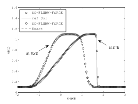
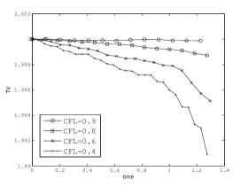
(a)	(b)

Figure 12: Solution corresponding to IC (67): (a) No clipping error for smooth extrema as well near shock zone $CFL=0.8,N=80$, (b) Effect of CFL on total variation diminishing plot of computed solution.

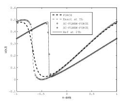
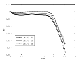
(a)	(b)

Figure 13: (a) Comparison of computed solution of corresponding to IC (68) at $Tb=1/4\pi$ $CFL=0.6,N=80$ (b) Total variation diminishing plot up to $t=2Tb$

		CFL=0.45				CFL=0.9
N	$L^{1}$ error	Rate	$L^{\infty}$ error	Rate	$L^{1}$ error	Rate	$L^{\infty}$ error	Rate
10	3.9495e-02	0.0000	1.0467e-02	0.0000	1.9593e-02	0.0000	4.7957e-03	0.0000
20	7.2108e-03	2.4534	1.8537e-03	2.4974	4.6493e-03	2.0753	1.1326e-03	2.0821
40	2.1212e-03	1.7653	3.7326e-04	2.3122	1.0845e-03	2.1000	2.4774e-04	2.1927
80	4.9995e-04	2.0850	7.0710e-05	2.4002	2.7441e-04	1.9826	4.2200e-05	2.5535
160	9.2620e-05	2.4324	1.7250e-05	2.0353	6.6870e-05	2.0369	8.3800e-06	2.3322
320	2.2230e-05	2.0588	4.1900e-06	2.0416	1.6580e-05	2.0119	1.7400e-06	2.2679
640	5.5900e-06	1.9916	1.0400e-06	2.0104	4.1900e-06	1.9844	3.6000e-07	2.2730

Table 7: Convergence rate for test case corresponding to IC (68) at pre-shock time $t=2/\pi$ $CFL=0.8$

6.3 Buckley Leverett Equation

Consider Buckley-Leverett equation which has convex-concave flux. This equation physically represents the flow of a mixture of oil and water through a porous medium.

$$\frac{\partial u}{\partial t}+\frac{\partial f(u)}{\partial x}=0$$ (69)

The flux function is given by,

$$f(u)=\frac{u^{2}}{u^{2}+\alpha(1-u)^{2}}.$$ (70)

Here $\alpha$ is viscosity ratio and $u$ represents the saturation of water and lies between $0$ and $1.$

6.3.1 One moving shock

Consider equation (69) with $\alpha=\frac{1}{2}$ and initial condition

$$u(x,\,0)=\left\{\begin{array}[]{ll}1,&x<0,\\ 0,&x>0.\end{array}\right.$$ (71)

The solution involves one single moving shock followed by an rarefaction wave.

6.3.2 Two moving shock

Consider equation (69) with $\alpha=\frac{1}{4}$ and subject to initial condition

$$u(x,\,0)=\left\{\begin{array}[]{ll}1,&-0.5\leq x\leq 0,\\ 0,&elsewhere.\end{array}\right.$$ (72)

The solution involves two moving shocks, each followed by an rarefaction wave. In numerical simulation flux limited high resolution LxW TVD scheme [31] is used in hybrid scheme 5.4 as CCS. The results corresponding IC (71) and (72) are given in Figure 14(a) and 14(b) respectively. Results show that the proposed scheme sharply captures both the fast and slow shocks. The rarefaction waves are also approximated with high resolution.

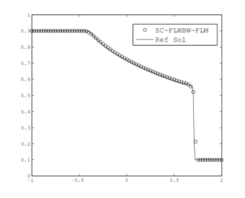
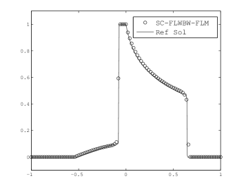
(a)	(b)

Figure 14: Numerical solution using $CFL=0.8$ (a) $N=80$ at time $t=0.75$ (b) $N=100$ at time $t=0.4$: Sharp resolution for rarefaction fans and slow and fast moving shocks.

6.4 1D Euler Equation

The 1D Euler equations of the Gas dynamics is given by

$$\frac{\partial}{\partial t}\textbf{u}+\frac{\partial}{\partial x}\textbf{F(u)}=0,$$ (73)

where $\textbf{u}=\left(\begin{array}[]{c}\rho\\ \rho u\\ E\end{array}\right)$ and $\textbf{F(u)}=\left(\begin{array}[]{c}\rho u\\ \rho u^{2}+p\\ (E+p)u\end{array}\right)$ denotes vector of conservative variables and conservative fluxes respectively. Variables $\rho,u$ and $p$ represents density, velocity and pressure respectively . The total energy $e$ is defined by,

$$e=\frac{p}{\gamma-1}+\frac{\rho u^{2}}{2}$$ (74)

where $\gamma$ is the ratio of specific heat coefficients. We consider the four shock tube problems modeled by (73) to check the robustness of proposed scheme in section 5.5. These shock tube tests check any method in capturing the contact and shock discontinuity along with non-oscillatory high resolution approximation for smooth extrema. In all the numerical test a simple high resolution TVD flux limited centered (FLIC) [40, 41] scheme with MINBEE limiter is used as CCS in 5.4. We denote results by this scheme by FLWBW-FLIC instead SC-FLWBW-FLIC. Numerical results are compared with FLIC to see the improvement in capturing the solution profile by FLWBW-FLIC. Note that, the MINBEE limiter satisfies the universal TVD stability region given in [8] and therefore robustly works for both positive and negative characteristics speed associated with system (73)

6.4.1 Shu-Osher shock tube test [3]

$$(\rho,u,p)=\begin{array}[]{ll}(3.857143,2.629369,10.3333)&x<-4.0,\\ (1+0.2\sin(5x),0,1)&x\geq-4.0.\end{array}$$ (75)

This test depicts shock interaction with a sine wave in density. The main challenge in this case is to capture both the complex small-scale smooth flow and shocks. In Figure 15 results are presented an compared with FLIC scheme. It is evident from zoomed figure 15(b) that the FLWBW-FLIC yields oscillation free approximation for shock with higher resolution compared to FLIC for complex oscillatory solution region about $[0.5,2.5]$. It also capture the smooth region in around $[-3,0.5]$ with out clipping or flattening error which is due to improved approximation of smooth extrema and steep gradient region.

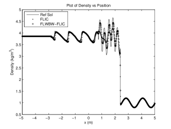
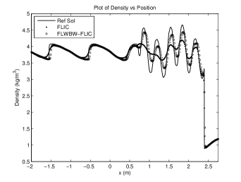
(a)	(b)

Figure 15: Numerical solution of shock entropy wave interaction $CFL=0.8,N=800$ using shock switch parameters $\epsilon=1\times 10^{-8},\delta=0.8$: high resolution of smooth extrema and steep gradient region.

6.4.2 Sod test tube

$$(\rho,u,p)=\begin{array}[]{ll}(1\;kg/m^{3},0\;m/s,100,000\;N/m^{2})&x<0\\ (0.125\;kg/m^{3},0\;m/s,10,000\;N/m^{2})&x\geq 0;\end{array},x\in[-10,10].$$ (76)

This test problem has no sonic point but the contact and shock are very close which cause a smeared approximation to the middle contact discontinuity. In Figure 16, numerical results are given and for different choice of shock switch parameters and compared with FLIC. Results show that proposed FLWBW-FLIC crisply captures the smooth rarefaction and contact discontinuity and shock more accurately than high order TVD scheme FLIC with Minbee limiter.

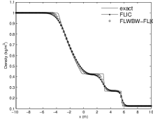
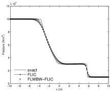
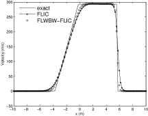
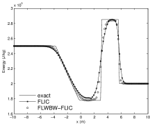
(a)	(b)

Figure 16: Solution Sod shock tube, $N=100,CFL=0.5$ after $67$ time steps at $T=0.01$ second with shock switch parameters $\epsilon=1\times 10^{-8}$, (a) $\delta=0.4$, (b) $\delta=0.9$

6.4.3 Lax Tube

$$(\rho,u,p)=\begin{array}[]{ll}(0.445\;kg/m^{3},0.698\;m/s,3.528\;N/m^{2})&x<1,\\ (0.5\;kg/m^{3},0\;m/s,0.571\;N/m^{2})&x\geq 1;\end{array}x\in[0,2].$$ (77)

Compared to Sod tube the shock in this case is very strong and mostly use to check the robustness of any schemes. In Figure 17 numerical results obtained by FLWBW-FLIC are given. It can be seen that that the method capture the contact and the rarefaction wave with higher resolution shock compared to FLIC for various choices of shock parameters.

(a)
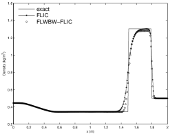
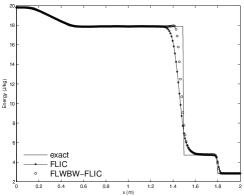
(b)
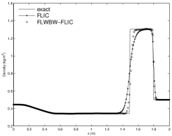
(c)
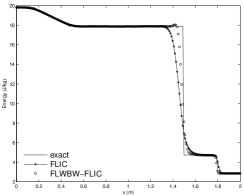
(d)

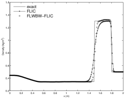
Figure 17: Density and energy plots Lax Shock tube case 2, $N=200,CFL=0.8$ after $187$ time steps at $T=0.32$ second with shock switch parameters in row (a) $\epsilon=1\times 10^{-2},\delta=0.2$, (b) $\epsilon=1\times 10^{-2},\delta=0.8$, (c) $\epsilon=1\times 10^{-4},\delta=0.4$ and (d) $\epsilon=1\times 10^{-8},\delta=0.8$.

6.4.4 Laney Test [20]

$$(\rho,u,p)=\begin{array}[]{ll}(1\;kg/m^{3},0\;m/s,100,000\;N/m^{2})&x<0,\\ (0.01\;kg/m^{3},0\;m/s,1,000\;N/m^{2})&x\geq 0;\end{array}x\in[-10,15].$$ (78)

In this test the density and pressure state on the right side of initial discontinuity is much smaller compared to the left state. Therefore computationally, even small oscillations can lead to negative density or pressure which results in to non-physical imaginary speed of sound $c=\sqrt{\frac{\gamma p}{\rho}}$. This makes it an important test to check the non-oscillatory nature of any numerical scheme. In Figure 18, the density and pressure plots obtained by FLWBW-FLIC are given and compared for shock switch parameters $\epsilon,\delta$.

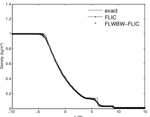
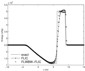
(a)	(b)

Figure 18: Solution Laney test, $N=200,CFL=0.8$ after $111$ time steps at $T=0.01$ second with shock switch parameters $\epsilon=1e-8$ (a) $\delta=0.6$ (b) $\delta=0.9$

Numerical results for 1D shock tube test problems show that the corners of rarefaction and contact discontinuities are better resolved by FLWBW-FLIC compared to centred flux limiter shock capturing TVD scheme FLIC. The shock is also crisply captured compared to to FLIC with Minbee limiter. The hybrid scheme presented in section 5.5 is robust and works for different choices of shock parameters $\epsilon,\;\delta$.

6.5 2D Euler Equation

Consider the two-dimensional Euler equations for compressible gas dynamics defined by the system

$$U_{t}+F(U)_{x}+G(U)_{y}=0,$$ (79)

where

$$U=\left(\begin{array}[]{cccc}\rho\\ \rho u\\ \rho v\\ e\end{array}\right),~{}F=\left(\begin{array}[]{cccc}\rho u\\ \rho u^{2}+p\\ \rho uv\\ u(e+p)\end{array}\right),~{}G=\left(\begin{array}[]{cccc}\rho v\\ \rho uv\\ \rho v^{2}+p\\ v(e+p)\end{array}\right)$$ (80)

Here $\rho$ is the density, $u$ and $v$ are velocity components in $x$ and $y$ direction respectively, $p$ is the pressure and $e$ is the energy defined by,

$$e=\frac{p}{\gamma-1}+\frac{\rho(u^{2}+v^{2})}{2}.$$ (81)

The Riemann problem for Euler equation (79) can be defined by considering the constant initial data in each quadrant of unit square $[0,1]\times[0,1]$ with center at $(0.5,0.5)$. More precisely consider (79) with initial data

$$(p,\rho,u,v)(x,y,t=0)=\left\{\begin{array}[]{cc}(p_{1},\rho_{1},u_{1},v_{1})&\mbox{if}\;x>0.5,y>0.5\\ (p_{2},\rho_{2},u_{2},v_{2})&\mbox{if}\;x<0.5,y>0.5\\ (p_{3},\rho_{3},u_{3},v_{3})&\mbox{if}\;x<0.5,y<0.5\\ (p_{4},\rho_{4},u_{4},v_{4})&\mbox{if}\;x>0.5,y<0.5\\ \end{array}\right.$$ (82)

In the 2D Riemann problems due to complex geometric wave pattern most high resolution schemes experience problems in yielding oscillations free crisp resolution to solution profile. Such 2D Riemann problem are numerically solved by using positive scheme and Riemann solvers free central schemes in [21] and [19] respectively. Recently some of the these Riemann problems are considered to see the performance of a new finite volume adaptive artificial viscosity method in [18] and (with slight changed geometry) a HLL Riemann solver in [43] respectively. In this section numerical results are given for twelve configurations. The one dimensional scheme presented in section 5.5 is extended to two dimensional Euler equation using the Strang dimension by dimension splitting technique. In Figure 19 to Figure 30 the contour plot of density are given and compared with FORCE scheme for different test cases. In all the figures contour plot by FORCE is given in column (a), and by FLWBW-FORCE in column (b) with shock parameters $\epsilon=1\times 10^{-8},\delta=0.6$. It is observed that small oscillations can occur with if a flux limited TVD scheme is used in hybrid scheme in section 5.5 (Results are not shown here). Note that it is in agreement with the comments in [19], that a over compressive Minmod type limiter can lead to spurious oscillations for the schemes proposed therein.

1. Configuration 1

   $$\begin{array}[]{llll}p_{1}=1&p_{2}=0.4&p_{3}=0.0439&p4=0.15\\ \rho_{1}=1&\rho_{2}=0.5197&\rho_{3}=0.1072&\rho_{4}=0.2579\\ u_{1}=0&u_{2}=-0.7259&u_{3}=-0.7259&u_{4}=0.0\\ v_{1}=0&v_{2}=0&v_{3}=-1.4045&v_{4}=-1.4045\\ \end{array}$$ (83)

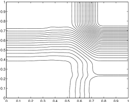
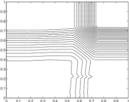
   (a)	(b)

   Figure 19: Configuration 1: Density contour plot (30 lines) at $T=0.2$, sharp resolution for rarefaction and ripple in lower rarefaction are sharply resolved in (b) compared to FORCE (a).

2. Configuration 2

   $$\begin{array}[]{llll}p_{1}=1&p_{2}=0.4&p_{3}=1&p_{4}=0.4\\ \rho_{1}=1&\rho_{2}=0.5197&\rho_{3}=1&\rho_{4}=0.5197\\ u_{1}=0&u_{2}=-0.7259&u_{3}=-0.7259&u_{4}=0\\ v_{1}=0&v_{2}=0&v_{3}=-0.7259&v_{4}=-0.7259\end{array}$$ (84)

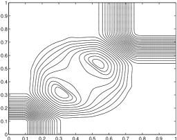
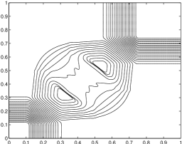
   (a)	(b)

   Figure 20: Configuration 2: Density contour plot (30 lines) at $T=0.25$ non-oscillatory sharp resolution for rarefaction waves and corners in (b) compared to FORCE in (a)

3. Configuration 3

   $$\begin{array}[]{llll}p_{1}=1.5&p_{2}=0.3&p_{3}=0.029&p_{4}=0.3\\ \rho_{1}=1.5&\rho 2=0.5323&\rho_{3}=0.138&\rho 4=0.5323\\ u_{1}=0&u_{2}=1.206&u_{3}=1.206&u_{4}=0\\ v_{1}=0&v_{2}=0&v_{3}=1.206&v_{4}=1.206\end{array}$$ (85)

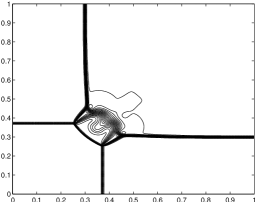
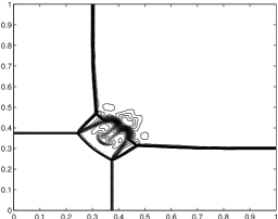
   (a)	(b)

   Figure 21: Configuration 3: Density contour plot (32 lines), All four shocks are sharply resolved with out induced oscillations in FLWBW-FORCE in (b) compared to FORCE in (a).

4. Configuration 4

   $$\begin{array}[]{llll}p_{1}=1.1&p_{2}=0.35&p_{3}=1.1&p_{4}=0.35\\ \rho_{1}=1.1&\rho_{2}=0.5065&\rho_{3}=1.1&\rho_{4}=0.5065\\ u_{1}=0&u_{2}=0.8939&u_{3}=0.8939&u_{4}=0\\ v_{1}=0&v_{2}=0&v_{3}=0.8939&v_{4}=0.8939\end{array}$$ (86)

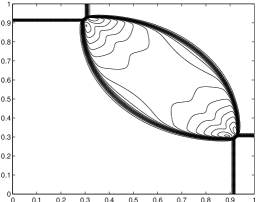
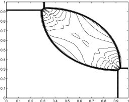
   (a)	(b)

   Figure 22: Configuration 4: Density contour plot (30 lines) non-oscillatory, FLWBW-FORCE yield sharp resolution for shocks in (b) compared to FORCE in (a)

5. Configuration 5

   $$\begin{array}[]{llll}p_{1}=1&p_{2}=1&p_{3}=1&p_{4}=1\\ \rho_{1}=1&\rho_{2}=2&\rho_{3}=1&\rho_{4}=3\\ u_{1}=-0.75&u_{2}=-0.75&u_{3}=0.75&u_{4}=0.75\\ v_{1}=-0.5&v_{2}=0.5&v_{3}=0.5&v_{4}=-0.5\end{array}$$ (87)

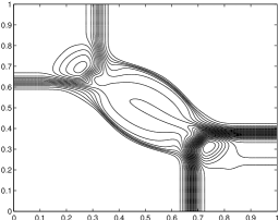
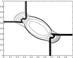
   (a)	(b)

   Figure 23: Configuration 5: Density plot (30 Lines) all four contacts are poorly resolved by FORCE (a), though FLWBW-FORCE yield sharp resolution to contacts with out oscillations in (b).

6. Configuration 6

   $$\begin{array}[]{llll}p_{1}=1&p_{2}=1&p_{3}=1&p_{4}=1\\ \rho_{1}=1&\rho_{2}=2&\rho_{3}=1&\rho_{4}=3\\ u_{1}=0.75&u_{2}=0.75&u_{3}=-0.75&u_{4}=-0.75\\ v_{1}=-0.5&v_{2}=0.5&v_{3}=0.5&v_{4}=-0.5\end{array}$$ (88)

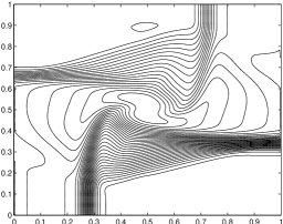
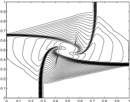
   (a)	(b)

   Figure 24: Configuration 6: The ripples in NE and SW quadrants are captured with comparable resolution with the one in [19] using FLWBW-FORCE (b) though the resolution for contacts is little diffusive but much sharper compared to FORCE (a).

7. Configuration 7

   $$\begin{array}[]{llll}p_{1}=1&p_{2}=0.4&p_{3}=0.4&p_{4}=0.4\\ \rho_{1}=1&\rho_{2}=0.5197&\rho_{3}=0.8&\rho_{4}=0.5197\\ u_{1}=0.1&u_{2}=-0.6259&u_{3}=0.1&u_{4}=0.1\\ v_{1}=0.1&v_{2}=0.1&v_{3}=0.1&v_{4}=-0.6259\\ \end{array}$$ (89)

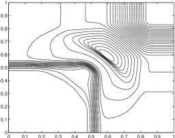
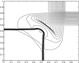
   (a)	(b)

   Figure 25: Configuration 7: The contacts in South and West are crisply resolved by FLWBW-FORCE (b). Moreover the rarefaction corners in NE quadrants are significantly sharper than FORCE (a).

8. Configuration 8

   $$\begin{array}[]{llll}p_{1}=0.4&p_{2}=1&p_{3}=1&p_{4}=1\\ \rho_{1}=0.5197&\rho_{2}=1&\rho_{3}=0.8&\rho_{4}=1\\ u_{1}=0.1&u_{2}=-0.6259&u_{3}=0.1&u_{4}=0.1\\ v_{1}=0.1&v_{2}=0.1&v_{3}=0.1&v_{4}=-0.6259\end{array}$$ (90)

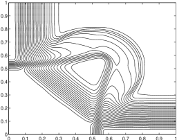
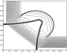
   (a)	(b)

   Figure 26: Configuration 8: The semi-circular wave front in NE is sharply resolved and resolution for contacts are comparable with the one in [19].

9. Configuration 9

   $$\begin{array}[]{llll}p_{1}=1&p_{2}=1&p_{3}=0.4&p_{4}=0.4\\ \rho 1=1&\rho 2=2&\rho 3=1.039&\rho 4=0.5197\\ u_{1}=0&u_{2}=0.0&u_{3}=0&u_{4}=0.0\\ v_{1}=0.3&v_{2}=-0.3&v_{3}=-0.8133&v_{4}=-0.4259\\ \end{array}$$ (91)

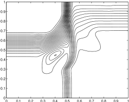
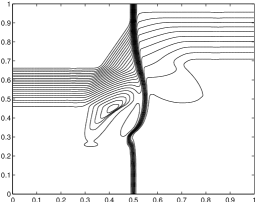
   (a)	(b)

   Figure 27: Configuration 9: Again rarefaction and corners are resolved sharper than FORCE (a). The vertical contact is crisply captured by FLWBW-FORCE.

10. Configuration 10

    $$\begin{array}[]{llll}p_{1}=1&p_{2}=1&p_{3}=0.3333&p_{4}=0.3333\\ \rho_{1}=1&\rho_{2}=0.5&\rho_{3}=0.2281&\rho_{4}=0.4562\\ u_{1}=0&u_{2}=0&u_{3}=0&u_{4}=0\\ v_{1}=0.4297&v_{2}=0.6076&v_{3}=-0.6076&v_{4}=-0.4297\end{array}$$ (92)

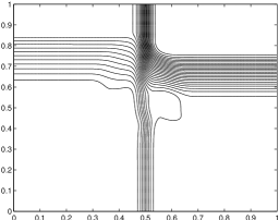
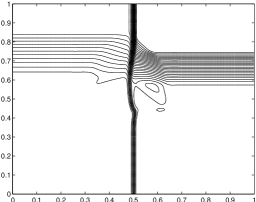
    (a)	(b)

    Figure 28: Configuration 10: Resolution of contacts by FLWBW-FORCE is comparable with the one in [19].

11. Configuration 11

    $$\begin{array}[]{llll}p_{1}=1&p_{2}=0.4&p_{3}=0.4&p_{4}=0.4\\ \rho_{1}=1&\rho_{2}=0.5313&\rho_{3}=0.8&\rho_{4}=0.5313\\ u_{1}=0.1&u_{2}=0.8276&u_{3}=0.1&u_{4}=0.1\\ v_{1}=0.0&v_{2}=0.0&v_{3}=0.0&v_{4}=0.7276\end{array}$$ (93)

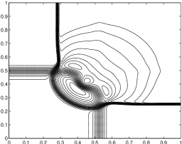
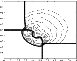
    (a)	(b)

    Figure 29: Configuration 11: Resolution of contact is SW quadrant, Shocks in SE and NW quadrants by FLWBW-FORCE (b) is better than that of the one in [19, 21].

12. Configuration 12

    $$\begin{array}[]{llll}p_{1}=0.4&p_{2}=1&p_{3}=1.0&p_{4}=1.0\\ \rho 1=0.5313&\rho 2=1.0222&\rho 3=0.8&\rho 4=1.0\\ u_{1}=0.1&u_{2}=-0.6179&u_{3}=0.1&u_{4}=0.1\\ v_{1}=0.1&v_{2}=0.1&v_{3}=0.1&v_{4}=0.8276\end{array}$$ (94)

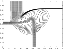
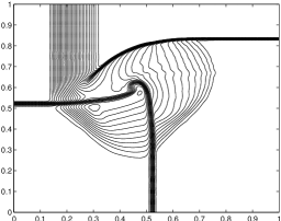
    (a)	(b)

    Figure 30: Configuration 12: FLWBW-FORCE recovers the ripples between NE shock and contact waves. The resolution for shock and contacts are comparable with the second order scheme results in [19].

Comments

7 Conclusion and Future work

In this work LMP/TVD bounds are obtained for uniformly second order accurate schemes in non-conservative form. These bound show that higher than second order TVD accuracy can be achieved at extrema and steep gradient region in limiting sense i.e., when $r\rightarrow 0^{-}$. Based on the LMP/TVD bounds hybrid local maximum principle satisfying schemes are constructed and applied on various benchmark test problems. Numerical results show improvement in TVD approximation of solution region with extreme points, smooth rarefaction as well contact discontinuity compared to existing higher order TVD method. For a separate work, the focus is on TVD bounds for multi-step methods and efficient use of a shock detector. As, the algorithm 5.4 recovered the shock at right location for scalar case, it would be interesting to devise a hybrid scheme for system by modifying the wave speed choice in section 5.5, with out a shock detector.

References

- [1] Michael Breuss. An analysis of the influence of data extrema on some first and second order central approximations of hyperbolic conservation laws. ESAIM: Mathematical Modelling and Numerical Analysis, 39(5):965–993, 3 2010.
- [2] Jameson, Antony. Positive schemes and shock modelling for compressible flows. International Journal for Numerical Methods in Fluids,20:743-776, 1995.
- [3] Shu Chi-Wang and Stanley Osher. Efficient implementation of essentially non-oscillatory shock-capturing schemes, ii. Journal of Computational Physics, 83:32–78, 1989.
- [4] Michael G. Crandall and Andrew Majda. Monotone difference approximations for scalar conservation laws. Mathematics of Computation, 34(149):1–21, jan 1980.
- [5] S. F. Davis. A simplified tvd finite difference scheme via artificial viscosity. SIAM J. Sci. and Stat. Comput., 8(1):pp. 1–18, 1987.
- [6] Bruno Després and Frédéric Lagoutière. Contact discontinuity capturing schemes for linear advection and compressible gas dynamics. Journal of Scientific Computing, 16(4):479–524, 2001.
- [7] Ritesh Kumar Dubey. Total variation stability and second-order accuracy at extrema. In Goddard Jerome and Zhu Jianping, editors, Ninth MSU-UAB Conference on Differential Equations and Computational Simulations, Electron. J. Diff. Eqns. Conf., pages 53–63, sept 2012.
- [8] Ritesh Kumar Dubey. Flux limited schemes: Their classification and accuracy based on total variation stability regions. Applied Mathematics and Computation, 224(0):325 – 336, 2013.
- [9] S. K. Godunov. A difference scheme for numerical solution of discontinuous solution of hydrodynamic equations, translated us joint publ. res. service, jprs 7225 nov. 29, 1960. Math. Sbornik, 47:271–306, 1959.
- [10] Jonathan B. Goodman and Randall J. LeVeque. A geometric approach to high resolution tvd schemes. SIAM J. Numer. Anal., 25:268–284, April 1988.
- [11] Ami Harten. High resolution schemes for hyperbolic conservation laws,. Journal of Computational Physics, 49(3):357 – 393, 1983.
- [12] Ami Harten. Eno schemes with subcell resolution. Journal of Computational Physics, 83(1):148 – 184, 1989.
- [13] Ami Harten and Peter D. Lax. On a class of high resolution total-variation-stable finite-difference schemes. SIAM Journal on Numerical Analysis, 21(1):pp. 1–23, 1984.
- [14] Thomas Y. Hou and Philippe G. Lefloch. Why nonconservative schemes converge to wrong weak solutions: Error analysis. Mathematics of Computation, 62(206), 1994.
- [15] S. Jaisankar and S.V. Raghurama Rao. A central rankine–hugoniot solver for hyperbolic conservation laws. Journal of Computational Physics, 228(3):770 – 798, 2009.
- [16] M.K. Kadalbajoo and Ritesh Kumar. A high resolution total variation diminishing scheme for hyperbolic conservation law and related problems. Applied Mathematics and Computation, 175(2):1556 – 1573, 2006.
- [17] Ritesh Kumar Dubey. A hybrid semi-primitive shock capturing scheme for conservation laws. Electron. J. Diff. Eqns., Eighth Mississippi State - UAB Conference on Differential Equations and Computational Simulations. Conference 19 (2010), pp. 65-73.
- [18] Alexander Kurganov and Yu Liu. New adaptive artificial viscosity method for hyperbolic systems of conservation laws. Journal of Computational Physics, 231(24):8114 – 8132, 2012.
- [19] Alexander Kurganov and Eitan Tadmor. Solution of two-dimensional riemann problems for gas dynamics without riemann problem solvers. Numerical Methods for Partial Differential Equations, 18(5):584–608, 2002.
- [20] Culbert B. Laney. Computational gasdynamics. Cambridge University Press, 1998.
- [21] Peter D. Lax and Xu-Dong Liu. Solution of two-dimensional riemann problems of gas dynamics by positive schemes. SIAM J. Sci. Comput., 19(2):319–340, March 1998.
- [22] Philippe G. Lefloch and Jian Guo Liu. Generalized monotone schemes, discrete paths of extrema, and discrete entropy conditions. Mathematics of Computation, 68:1025–1055, 1999.
- [23] Sanjiva K. Lele. Compact finite difference schemes with spectral-like resolution. Journal of Computational Physics, 103(1):16–42, November 1992.
- [24] Randall J. LeVeque. Numerical Methods for Conservation Laws. Lectures in mathematics ETH Zürich. Birkhäuser Basel, 2nd edition, February 1992.
- [25] J. Li and Z. Yang. Heuristic modified equation analysis on oscillations in numerical solutions of conservation laws. SIAM Journal on Numerical Analysis, 49(6):2386–2406, 2011.
- [26] Jiequan Li, Huazhong Tang, Gerald Warnecke, and Lumei Zhang. Local oscillations in finite difference solutions of hyperbolic conservation laws. Math. Comput., 78(268):1997–2018, 2009.
- [27] M. Oliveira, P. Lu, X. Liu, and C. Liu. A new shock/discontinuity detector. International Journal of Computer Mathematics, 87(13):3063–3078, 2010.
- [28] S. Osher and S. Chakravarthy. High resolution schemes and entropy condition. SIAM J. Numer. Anal., 21:955–984, 1984.
- [29] Stanley Osher and Eitan Tadmor. On the convergence of difference approximations to scalar conservation laws. Mathematics of Computation, 50(181):pp. 19–51, 1988.
- [30] Serge Piperno and Sophie Depeyre. Criteria for the design of limiters yielding efficient high resolution tvd schemes. Computers & Fluids, 27(2):183 – 197, 1998.
- [31] William J. Rider. A comparison of tvd lax-wendroff methods. Communications in Numerical Methods in Engineering, 9(2):147–155, 1993.
- [32] Philip L Roe. Some contributions to the modelling of discontinuous flows. In Large-scale computations in fluid mechanics, volume 1, pages 163–193, 1985.
- [33] Richard Sanders. On convergence of monotone finite difference schemes with variable spatial differencing. Mathematics of Computation, 40(161):91–106, Jan 1983.
- [34] Richard Sanders. A third-order accurate variation nonexpansive difference scheme for single nonlinear conservation laws. Mathematics of Computation, 51(184):pp. 535–558, 1988.
- [35] Chi-Wang Shu. High order eno and weno schemes for computational fluid dynamics. In TimothyJ. Barth and Herman Deconinck, editors, High-Order Methods for Computational Physics, volume 9 of Lecture Notes in Computational Science and Engineering, pages 439–582. Springer Berlin Heidelberg, 1999.
- [36] Chi-Wang Shu. Efficient algorithms for solving partial differential equations with discontinuous solutions. Notices of the AMS, 59(5), 2012.
- [37] G.A. Sod. Survey of several finite difference methods for systems of nonlinear hyperbolic conservation laws. Journal of Computational Physics, Apr 1978.
- [38] P. K. Sweby. High resolution schemes using flux limiters for hyperbolic conservation laws. Siam Journal on Numerical Analysis, 21(5):995–1011, 1984.
- [39] J W. Thomas. Numerical partial differential equations- conservation laws and elliptic equations. Texts in Applied Mathematics 33. Springer-Verlag, 1999.
- [40] EF Toro and SJ Billett. Centred tvd schemes for hyperbolic conservation laws. IMA Journal of Numerical Analysis, 20(1):47–79, 2000.
- [41] Eleuterio F. Toro. Riemann Solvers and Numerical Methods for Fluid Dynamics: A Practical Introduction. Springer, 3rd edition, April 2009.
- [42] Bram van Leer. Towards the ultimate conservative difference scheme. ii. monotonicity and conservation combined in a second-order scheme. Journal of Computational Physics, 14(4):361 – 370, 1974.
- [43] Jeaniffer Vides, Boniface Nkonga, and Edouard Audit. A simple two-dimensional extension of the {HLL} riemann solver for hyperbolic systems of conservation laws. Journal of Computational Physics, 280(0):643 – 675, 2015.
- [44] H. Yang. On wavewise entropy inequalities for high-resolution schemes. i: the semidiscrete case. Math. Comp., 65:45–67, 1996.
- [45] H. C. Yee. Construction of explicit and implicit symmetric tvd schemes and their applications. Journal of Computational Physics, 68(1):151 – 179, 1987.
- [46] X. Zhang and C-W Shu. Maximum-principle-satisfying and positivity-preserving high-order schemes for conservation laws: survey and new developments. Proc. R. Soc. A, 467:2752–2776, 2011.
- [47] Xiangxiong Zhang and Chi-Wang Shu. A genuinely high order total variation diminishing scheme for one-dimensional scalar conservation laws. SIAM J. Numerical Analysis, 48(2):772–795, 2010.
- [48] Xiangxiong Zhang and Chi-Wang Shu. On maximum-principle-satisfying high order schemes for scalar conservation laws. Journal of Computational Physics, 229(9):3091 – 3120, 2010.