Adaptive-Rate Sparse Signal Reconstruction With Application in Compressive Background Subtraction

Abstract

We propose and analyze an online algorithm for reconstructing a sequence of signals from a limited number of linear measurements. The signals are assumed sparse, with unknown support, and evolve over time according to a generic nonlinear dynamical model. Our algorithm, based on recent theoretical results for $\ell_{1}$-$\ell_{1}$ minimization, is recursive and computes the number of measurements to be taken at each time on-the-fly. As an example, we apply the algorithm to compressive video background subtraction, a problem that can be stated as follows: given a set of measurements of a sequence of images with a static background, simultaneously reconstruct each image while separating its foreground from the background. The performance of our method is illustrated on sequences of real images: we observe that it allows a dramatic reduction in the number of measurements with respect to state-of-the-art compressive background subtraction schemes.

I Introduction

Consider the problem of reconstructing a sequence of sparse signals from a limited number of measurements. Let $x[k]\in\mathbb{R}^{n}$ be the signal at time $k$ and $y[k]\in\mathbb{R}^{m_{k}}$ be the vector of signal measurements at time $k$, where $m_{k}\ll n$. Assume the signals evolve according to the dynamical model

$$x[k] =f_{k}\big{(}\{x[i]\}_{i=1}^{k-1}\big{)}+\epsilon[k]$$ (1a)

$$y[k] =A_{k}\,x[k]\,,$$ (1b)

where $\epsilon[k]\in\mathbb{R}^{n}$ is modeling noise and $A_{k}\in\mathbb{R}^{m_{k}\times n}$ is a sensing matrix. In (1a), $f_{k}:(\mathbb{R}^{n})^{k-1}\xrightarrow{}\mathbb{R}^{n}$ is a known, but otherwise arbitrary, map that describes $x[k]$ as a function of past signals. We assume that each $x[k]$ and $\epsilon[k]$ is sparse, i.e., it has a small number of nonzero entries. Our goal is to reconstruct the signal sequence $\{x[k]\}$ from the measurement sequence $\{y[k]\}$. We require the reconstruction scheme to be recursive (or online), i.e., $x[k]$ is reconstructed before acquiring measurements of any future signal $x[i]$, $i>k$, and also to use a minimal number of measurements. We formalize the problem as follows.

Problem statement. Given two unknown sparse sequences $\{x[k]\}$ and $\{\epsilon[k]\}$ satisfying (1), design an online algorithm that 1) uses a minimal number of measurements $m_{k}$ at time $k$, and 2) perfectly reconstructs each $x[k]$ from $y[k]$ acquired as in (1b), and possibly $x[i]$, $i<k$.

Note that our setting immediately generalizes from the case where each $x[k]$ is sparse to the case where $x[k]$ has a sparse representation in a linear, invertible transform.

I-A Applications

Many problems require estimating a sequence of signals from a sequence of measurements satisfying the model in (1). These include classification and tracking in computer vision systems [2, 3], radar tracking [4], dynamic MRI [5] and several tasks in wireless sensor networks [6].

Our application focus, however, is compressive background subtraction [7]. Background subtraction is a key task for detecting and tracking objects in a video sequence and it has been applied, for example, in video surveillance [8, 9], traffic monitoring [10, 11], and medical imaging [12, 13]. Although there are many background subtraction techniques, e.g., [14, 3, 15], most of them assume access to full frames and, thus, are inapplicable in compressive video sensing [16, 17, 18], a technology used in cameras where sensing is expensive (e.g., infrared, UV wavelengths).

In compressive video sensing, one has access not to full frames as in conventional video, but only to a small set of linear measurements of each frame, as in (1b). Cevher et al. [7] noticed that background subtraction is possible in this context if the foreground pixels, i.e., those associated to a moving object, occupy a small area in each frame. Assuming the background image is known beforehand, compressed sensing techniques [19, 20] such as $\ell_{1}$-norm minimization allow reconstructing each foreground. This not only reconstructs the original frame (if we add the reconstructed foreground to the known background), but also performs background subtraction as a by-product [7].

We mention that, with the exception of [21, 22], most approaches to compressive video sensing and to compressive background subtraction assume a fixed number of measurements for all frames [16, 7, 23, 24, 17, 18]. If this number is too small, reconstruction of the frames fails. If it is too large, reconstruction succeeds, but at the cost of spending unnecessary measurements in some or all frames. The work in [21, 22] addresses this problem with an online scheme that uses cross validation to compute the number of required measurements. Given a reconstructed foreground, [21, 22] estimates the area of the true foreground using extra cross-validation measurements. Then, assuming that foreground areas of two consecutive frames are the same, the phase diagram of the sensing matrix, which was computed beforehand, gives the number of measurements for the next frame. This approach, however, fails to use information from past frames in the reconstruction process, information that, as we will see, can be used to significantly reduce the number of measurements.

I-B Overview of our approach and contributions

Overview. Our approach to adaptive-rate signal reconstruction is based on the recent theoretical results of [25, 26]. These characterize the performance of sparse reconstructing schemes in the presence of side information. The scheme we are most interested in is the $\ell_{1}$-$\ell_{1}$ minimization:

$$\begin{array}[t]{ll}\underset{x}{\text{minimize}}&\|x\|_{1}+\beta\|x-w\|_{1}\\ \text{subject to}&Ax=y\,,\end{array}$$ (2)

where $x\in\mathbb{R}^{n}$ is the optimization variable and $\|x\|_{1}:=\sum_{i=1}^{n}|x_{i}|$ is the $\ell_{1}$-norm. In (2), $y\in\mathbb{R}^{m}$ is a vector of measurements and $\beta$ is a positive parameter. The vector $w\in\mathbb{R}^{n}$ is assumed known and is the so-called prior or side information: a vector similar to the vector that we want to reconstruct, say $x^{\star}$. Note that if we set $\beta=0$ in (2), we obtain basis pursuit [27], a well-known problem for reconstructing sparse signals and which is at the core of the theory of compressed sensing [20, 19]. Problem (2) generalizes basis pursuit by integrating the side information $w$. The work in [25, 26] shows that, if $w$ has reasonable quality and the entries of $A$ are drawn from an i.i.d. Gaussian distribution, the number of measurements required by (2) to reconstruct $x^{\star}$ is much smaller than the number of measurements required by basis pursuit. Furthermore, the theory in [25, 26] establishes that $\beta=1$ is an optimal choice, irrespective of any problem parameter. This makes the reconstruction problem (2) parameter-free.

We address the problem of recursively reconstructing a sequence of sparse signals satisfying (1) as follows. Assuming the measurement matrix is Gaussian, we propose an algorithm that uses (2) with $w=f_{k}\big{(}\{x[i]\}_{i=1}^{k-1}\big{)}$ to reconstruct each signal $x[k]$. And, building upon the results of [25, 26], we equip our algorithm with a mechanism to automatically compute an estimate on the number of required measurements. As application, we consider compressive background subtraction and show how to generate side information from past frames.

Contributions. We summarize our contributions as follows:

• We propose an adaptive-rate algorithm for reconstructing sparse sequences satisfying the model in (1).

• We establish conditions under which our algorithm reconstructs a finite sparse sequence $\{x[i]\}_{i=1}^{k}$ with large probability.

• We describe how to apply the algorithm to compressive background subtraction problems, using motion-compensated extrapolation to predict the next image to be acquired. In other words, we show how to generate side information.

• Given that images predicted by motion-compensated extrapolation are known to exhibit Laplacian noise, we then characterize the performance of (2) under this model.

• Finally, we show the impressive performance of our algorithm for performing compressive background subtraction on a sequence of real images.

Besides the incorporation of a scheme to compute a minimal number of measurements on-the-fly, there is another aspect that makes our algorithm fundamentally different from prior work. As overviewed in Section II, most prior algorithms for reconstructing dynamical sparse signals work well only when the sparsity pattern of $x[k]$ varies slowly with time. Our algorithm, in contrast, operates well even when the sparsity pattern of $x[k]$ varies arbitrarily between consecutive time instants, as shown by our theory and experiments. What is required to vary slowly is the “quality” of the prediction given by each $f_{k}$ (i.e., the quality of the side information) and, to a lesser extent, not the sparsity pattern of $x[k]$ but only its sparsity, i.e., the number of nonzero entries.

I-C Organization

Section II overviews related work. In Section III, we state the results from [25, 26] that are used by our algorithm. Section IV describes the algorithm and establishes reconstruction guarantees. Section V concerns the application to compressive background subtraction. Experimental results illustrating the performance of our algorithm are shown in section VI; and section VII concludes the paper. The appendix contains the proofs of our results.

II Related work

There is an extensive literature on reconstructing time-varying signals from limited measurements. Here, we provide an overview by referring a few landmark papers.

The Kalman filter. The classical solution to estimate a sequence of signals satisfying (1) or, in the control terminology, the state of a dynamical system, is the Kalman filter [30]. The Kalman filter is an online algorithm that is least-squares optimal when the model is linear, i.e., $f_{k}\big{(}\{x[i]\}_{i=0}^{k-1}\big{)}=F_{k}x[k]$, and the sequence $\{\epsilon[k]\}$ is Gaussian and independent across time. Several extensions are available when these assumptions do not hold [31, 32, 33]. The Kalman filter and its extensions, however, are inapplicable to our scenario, as they do not easily integrate the additional knowledge that the state is sparse.

Dynamical sparse signal reconstruction. Some prior work incorporates signal structure, such as sparsity, into online sparse reconstruction procedures. For example, [34, 35] adapts a Kalman filter to estimate a sequence of sparse signals. Roughly, we have an estimate of the signal’s support at each time instant and use the Kalman filter to compute the (nonzero) signal values. When a change in the support is detected, the estimate of the support is updated using compressed sensing techniques. The work in [34, 35], however, assumes that the support varies very slowly and does not provide any strategy to update (or compute) the number of measurements; indeed, the number of measurements is assumed constant along time. Related work that also assumes a fixed number of measurements includes [36], which uses approximate belief propagation, and [37], which integrates sparsity knowledge into a Kalman filter via a pseudo-measurement technique. The works in [38, 39] and [40] propose online algorithms named GROUSE and PETRELS, respectively, for estimating signals that lie on a low-dimensional subspace. Their model can be seen as a particular case of (1), where each map $f_{k}$ is linear and depends only on the previous signal. Akin to most prior work, both GROUSE and PETRELS assume that the rank of the underlying subspace (i.e., the sparsity of $x[k]$) varies slowly with time, and fail to provide a scheme to compute the number of measurements.

We briefly overview the work in [41], which is probably the closest to ours. Three dynamical reconstruction schemes are studied in [41]. The one with the best performance is

$$\underset{x}{\text{minimize}}\,\,\|x\|_{1}+\beta\|x-w\|_{1}+\beta_{2}\|Ax-y\|_{2}^{2}\,,$$ (3)

where $\beta_{2}>0$ and $\|\cdot\|_{2}$ is the Euclidean $\ell_{2}$-norm. Problem (3) is the Lagrangian version of the problem we obtain by replacing the constraints of (2) with $\|Ax-y\|_{2}\leq\sigma$, where $\sigma$ is a bound on the measurement noise; see problem (9) below. For $\beta_{2}$ in a given range, the solutions of (9) and (3) coincide. This is why the approach in [41] is so closely related to ours. Nevertheless, using (9) has two important advantages: first, in practice, it is easier to obtain bounds on the measurement noise $\sigma$ than it is to tune $\beta_{2}$; second, and more importantly, the problem in (9) has well-characterized reconstruction guarantees [25, 26]. It is exactly those guarantees that enable our scheme for computing of the number of measurements online. The work in [41], as most prior work, assumes a fixed number of measurements for all signals.

III Preliminaries: Static signal
reconstruction using $\ell_{1}$-$\ell_{1}$ minimization

This section reviews some results from [25], namely reconstruction guarantees for (2) in a static scenario, i.e., when we estimate just one signal, not a sequence. As mentioned before, $\beta=1$ is an optimal choice: it not only minimizes the bounds in [25], but also leads to the best results in practice. This is the reason why we use $\beta=1$ henceforth.

$\ell_{1}$-$\ell_{1}$ minimization. Let $x^{\star}\in\mathbb{R}^{n}$ be a sparse vector, and assume we have $m$ linear measurements of $x^{\star}$: $y=Ax^{\star}$, where $A\in\mathbb{R}^{m\times n}$. Denote the sparsity of $x^{\star}$ with $s:=|\{i\,:\,x_{i}^{\star}\neq 0\}|$, where $|\cdot|$ is the cardinality of a set. Assume we have access to a signal $w\in\mathbb{R}^{n}$ similar to $x^{\star}$ (in the sense that $\|x^{\star}-w\|_{1}$ is small) and suppose we attempt to reconstruct $x^{\star}$ by solving the $\ell_{1}$-$\ell_{1}$ minimization problem (2) with $\beta=1$:

$$\begin{array}[t]{ll}\underset{x}{\text{minimize}}&\|x\|_{1}+\|x-w\|_{1}\\ \text{subject to}&Ax=y\,.\end{array}$$ (4)

The number of measurements that problem (4) requires to reconstruct $x^{\star}$ is a function of the “quality” of the side information $w$. Quality in [25] is measured in terms of the following parameters:

$$\xi :=\big{|}\{i\,:\,w_{i}\neq x_{i}^{\star}=0\}\big{|}-\big{|}\{i\,:\,w_{i}=x_{i}^{\star}\neq 0\}\big{|}\,,$$ (5a)

$$\overline{h} :=\big{|}\{i\,:\,x_{i}^{\star}>0,\,\,x_{i}^{\star}>w_{i}\}\cup\{i\,:\,x_{i}^{\star}<0,\,\,x_{i}^{\star}<w_{i}\}\big{|}\,.$$ (5b)

Note that the number of components of $w$ that contribute to $\overline{h}$ are the ones defined on the support of $x^{\star}$; thus, $0\leq\overline{h}\leq s$.

Theorem 1 (Th. 1 in [25]).

Let $x^{\star},w\in\mathbb{R}^{n}$ be the vector to reconstruct and the side information, respectively. Assume $\overline{h}>0$ and that there exists at least one index $i$ for which $x_{i}^{\star}=w_{i}=0$. Let the entries of $A\in\mathbb{R}^{m\times n}$ be i.i.d. Gaussian with zero mean and variance $1/m$. If

$$m\geq 2\overline{h}\log\Big{(}\frac{n}{s+\xi/2}\Big{)}+\frac{7}{5}\Big{(}s+\frac{\xi}{2}\Big{)}+1\,,$$ (6)

then, with probability at least $1-\exp\big{(}-\frac{1}{2}(m-\sqrt{m})^{2}\big{)}$, $x^{\star}$ is the unique solution of (4).

Theorem 1 establishes that if the number of measurements is larger than (6) then, with high probability, (4) reconstructs $x^{\star}$ perfectly. The bound in (6) is a function of the signal dimension $n$ and sparsity $s$, and of the quantities $\xi$ and $\overline{h}$, which depend on the signs of the entries of $x^{\star}$ and $w-x^{\star}$, but not on their magnitudes. When $w$ approximates $x^{\star}$ reasonably well, the bound in (6) is much smaller than the one for basis pursuit in [42]:

$$m\geq 2s\log\Big{(}\frac{n}{s}\Big{)}+\frac{7}{5}s+1\,.$$ (7)

Namely, [42] establishes that if (7) holds and if $A\in\mathbb{R}^{m\times n}$ has i.i.d. Gaussian entries with zero mean and variance $1/m$ then, with probability similar to the one in Theorem 1, $x^{\star}$ is the unique solution to basis pursuit. Indeed, if $\overline{h}\ll s$ and $\xi$ is larger than a small negative constant, then (6) is much smaller than (7). Note that, in practice, the quantities $s$, $\xi$, and $\overline{h}$ are unknown, since they depend on the unknown signal $x^{\star}$. In the next section, we propose an online scheme to estimate them using past signals.

Noisy case. Theorem 1 has a counterpart for noisy measurements, which we state informally; see [25] for details. Let $y=Ax^{\star}+\eta$, where $\|\eta\|_{2}\leq\sigma$. Let also $A\in\mathbb{R}^{m\times n}$ be as in Theorem 1 with

$$m\geq\frac{1}{(1-\tau)^{2}}\bigg{[}2\overline{h}\log\Big{(}\frac{n}{s+\xi/2}\Big{)}+\frac{7}{5}\Big{(}s+\frac{\xi}{2}\Big{)}+\frac{3}{2}\bigg{]}\,,$$ (8)

where $0<\tau<1$. Let $\hat{x}_{\text{noisy}}$ be any solution of

$$\begin{array}[t]{ll}\underset{x}{\text{minimize}}&\|x\|_{1}+\beta\|x-w\|_{1}\\ \text{subject to}&\|Ax-y\|_{2}\leq\sigma\,.\end{array}$$ (9)

Then, with overwhelming probability, $\|\hat{x}_{\text{noisy}}-x^{\star}\|_{2}\leq 2\sigma/\tau$, i.e., (9) reconstructs $x^{\star}$ stably. Our algorithm, described in the next section, adapts easily to the noisy scenario, but we provide reconstruction guarantees only for the noiseless case.

Algorithm 1 Adaptive-Rate Sparse Signal Reconstruction

1:$0\leq\alpha\leq 1$, a positive sequence $\{\delta_{k}\}$, and estimates $\hat{s}_{1}$ and $\hat{s}_{2}$ of the sparsity of $x[1]$ and $x[2]$, respectively.

2:

3:

4:for the first two time instants $k=1,2$ do

5:    Set $m_{k}=2\hat{s}_{k}\log(n/\hat{s}_{k})+(7/5)\hat{s}_{k}+1$

6:    Generate Gaussian matrix $A_{k}\in\mathbb{R}^{m_{k}\times n}$

7:    Acquire $m_{k}$ measurements of $x[k]$: $y[k]=A_{k}\,x[k]$

8:    Find $\hat{x}[k]$ such that

$$\hat{x}[k]\in\begin{array}[t]{cl}\underset{x}{\arg\min}&\|x\|_{1}\\ \text{s.t.}&A_{k}\,x=y[k]\end{array}$$

9:end for

10:Set $w[2]=f_{2}(\hat{x}[1])$ and compute

$$\hat{\xi}_{2} :=\big{|}\{i\,:\,w_{i}[2]\neq\hat{x}_{i}[2]=0\}\big{|}-\big{|}\{i\,:\,w_{i}[2]=\hat{x}_{i}[2]\neq 0\}\big{|}$$

$$\hat{\overline{h}}_{2} :=\big{|}\{i\,:\,\hat{x}_{i}[2]>0,\,\,\hat{x}_{i}[2]>w_{i}[2]\}\cup\{i\,:\,\hat{x}_{i}[2]<0,$$

$$\qquad\qquad\qquad\qquad\qquad\qquad\qquad\qquad\qquad\hat{x}_{i}[2]<w_{i}[2]\}\big{|}\,.$$

11:Set $\hat{\overline{m}}_{2}=2\hat{\overline{h}}_{2}\log\big{(}n/(\hat{s}_{2}+\hat{\xi}_{2}/2)\big{)}+(7/5)\big{(}\hat{s}_{2}+\hat{\xi}_{2}/2\big{)}+1$

12:Set $\phi_{3}=\hat{\overline{m}}_{2}$

13:

14:

15:for each time instant $k=3,4,5,\ldots$ do

16:    Set $m_{k}=(1+\delta_{k})\phi_{k}$

17:    Generate Gaussian matrix $A_{k}\in\mathbb{R}^{m_{k}\times n}$

18:    Acquire $m_{k}$ measurements of $x[k]$: $y[k]=A_{k}\,x[k]$

19:    Set $w[k]=f_{k}(\{\hat{x}[i]\}_{i=1}^{k-1})$ and find $\hat{x}[k]$ such that

$$\hat{x}[k]\in\begin{array}[t]{cl}\underset{x}{\arg\min}&\|x\|_{1}+\big{\|}x-w[k]\big{\|}_{1}\\ \text{s.t.}&A_{k}\,x=y[k]\end{array}$$

20:    Compute

$$\hat{s}_{k} =|\{i\,:\,\hat{x}[k]\neq 0\}|$$

$$\hat{\xi}_{k} =\big{|}\{i\,:\,w_{i}[k]\neq\hat{x}_{i}[k]=0\}\big{|}-\big{|}\{i\,:\,w_{i}[k]=\hat{x}_{i}[k]\neq 0\}\big{|}$$

$$\hat{\overline{h}}_{k} =\big{|}\{i\,:\,\hat{x}_{i}[k]>0,\,\,\hat{x}_{i}[k]>w_{i}[k]\}\cup\{i\,:\,\hat{x}_{i}[k]<0,$$

$$\qquad\qquad\qquad\qquad\qquad\qquad\qquad\qquad\qquad\hat{x}_{i}[k]<w_{i}[k]\}\big{|}\,.$$

21:    Set $\hat{\overline{m}}_{k}=2\hat{\overline{h}}_{k}\log\big{(}n/(\hat{s}_{k}+\hat{\xi}_{k}/2)\big{)}+(7/5)\big{(}\hat{s}_{k}+\hat{\xi}_{k}/2\big{)}+1$

22:    Update $\phi_{k+1}=(1-\alpha)\phi_{k}+\alpha\,\hat{\overline{m}}_{k}$

23:end for

IV Online sparse signal estimation

Algorithm 1 describes our online scheme for reconstructing a sparse sequence $\{x[k]\}$ satisfying (1). Although described for a noiseless measurement scenario, the algorithm adapts to the noisy scenario in a straightforward way, as discussed later. Such an adaptation is essential when using it on a real system, e.g., a single-pixel camera [43].

IV-A Algorithm description

The algorithm consists of two parts: the initialization, where the first two signals $x[1]$ and $x[2]$ are reconstructed using basis pursuit, and the online estimation, where the remaining signals are reconstructed using $\ell_{1}$-$\ell_{1}$ minimization.

Part I: Initialization. In steps 4-9, we compute the number of measurements $m_{1}$ and $m_{2}$ according to the bound in (7), and then reconstruct $x[1]$ and $x[2]$ via basis pursuit. The expressions for $m_{1}$ and $m_{2}$ in step 5 require estimates $\hat{s}_{1}$ and $\hat{s}_{2}$ of the sparsity of $x[1]$ and $x[2]$, which are given as input to the algorithm. Henceforth, variables with hats refer to estimates. Steps 10-12 initialize the estimator $\phi_{k}$: during Part II of the algorithm, $\phi_{k}$ should approximate the right-hand side of (6) for $x[k]$, i.e., with $s=s_{k}$, $\overline{h}=\overline{h}_{k}$, and $\xi=\xi_{k}$, where the subscript $k$ indicates that these are parameters associated with $x[k]$.

Part II: Online estimation. The loop in Part II starts by computing the number of measurements as $m_{k}=(1+\delta_{k})\phi_{k}$, where $\delta_{k}$, an input to the algorithm, is a (positive) safeguard parameter. We take more measurements from $x[k]$ than the ones prescribed by $\phi_{k}$, because $\phi_{k}$ is only an approximation to the bound in (6), as explained next. After acquiring measurements from $x[k]$, we reconstruct it as $\hat{x}[k]$ via $\ell_{1}$-$\ell_{1}$ minimization with $w[k]=f_{k}(\{\hat{x}[i]\}_{i=1}^{k-1})$ (step 19). Next, in step 20, we compute the sparsity $\hat{s}_{k}$ and the quantities in (5), $\hat{\xi}_{k}$ and $\hat{\overline{h}}_{k}$, for $\hat{x}[k]$. If the reconstruction of $x[k]$ is perfect, i.e., $\hat{x}[k]=x[k]$, then all these quantities match their true values. In that case, $\hat{\overline{m}}_{k}$ in step 21 will also match the true value of the bound in (6). Note, however, that the bound for $x[k]$, $\hat{\overline{m}}_{k}$, is computed only after $x[k]$ is reconstructed. Consequently, the number of measurements used in the acquisition of $x[k]$, $k>2$, is a function of the bound (6) for $x[k-1]$. Since the bounds for $x[k]$ and $x[k-1]$ might differ, we take more measurements than the ones specified by $\phi_{k}$ by a factor $\delta_{k}$, as in step 16. Also, we mitigate the effect of failed reconstructions by filtering $\hat{\overline{m}}_{k}$ with an exponential moving average filter, in step 22. Indeed, if reconstruction fails for some $x[k]$, the resulting $\hat{\overline{m}}_{k}$ might differ significantly from the true bound in (6). The role of the filter is to smooth out such variations.

Extension to the noisy case. Algorithm 1 can be easily extended to the scenario where the acquisition process is noisy, i.e., $y[k]=A_{k}x[k]+\eta_{k}$. Assume that $\eta_{k}$ is arbitrary noise, but has bounded magnitude, i.e., we know $\sigma_{k}$ such that $\|\eta_{k}\|_{2}\leq\sigma_{k}$. In that case, the constraint in the reconstruction problems in steps 8 and 19 should be replaced by $\|A_{k}x-y[k]\|_{2}\leq\sigma_{k}$. The other modification is in steps 11 and 21, whose expressions for $\hat{\overline{m}}_{k}$ are multiplied by $1/(1-\tau)^{2}$ as in (8). Our reconstruction guarantees, however, hold only for the noiseless case.

Remarks. We will see in the next section that Algorithm 1 works well when each $\delta_{k}$ is chosen according to the prediction quality of $f_{k}$: the worse the prediction quality, the larger $\delta_{k}$ should be. In practice, it may be more convenient to make $\delta_{k}$ constant, as we do in our experiments in Section VI. Note that the conditions under which our algorithm performs well differ from the majority of prior work. For example, the algorithms in [34, 35, 7, 36, 21, 37, 44, 40, 38, 39, 22] work well when the sparsity pattern of $x[k]$ varies slowly between consecutive time instants. Our algorithm, in contrast, works well when the quality parameters $\xi_{k}$ and $\overline{h}_{k}$ of the side information and also the sparsity $s_{k}$ of $x[k]$ vary slowly; in other words, when the quality of the prediction of $f_{k}$ varies slowly.

IV-B Reconstruction guarantees

The following result bounds the probability with which Algorithm 1 with $\alpha=1$ perfectly reconstructs a finite-length sequence $\{x[i]\}_{i=1}^{k}$. The idea is to rewrite the condition that (6) applied to $x[i-1]$ is $(1+\delta_{i})$ times larger than (6) applied to $x[i]$. If that condition holds for the entire sequence then, using Theorem 1 and assuming that the matrices $A_{k}$ are drawn independently, we can bound the probability of successful reconstruction. The proof is in Appendix A.

Lemma 2.

Let $\alpha=1$, $\underline{m}:=\min\big{\{}m_{1},m_{2},\min_{i=3,\ldots,k}\hat{\overline{m}}_{i}\big{\}}$, and fix $k>2$. Let also, for all $i=3,\ldots,k$,

$$\delta_{i}\geq\frac{2\big{[}\overline{h}_{i}\log(\frac{n}{u_{i}})-\overline{h}_{i-1}\log(\frac{n}{u_{i-1}})\big{]}+\frac{7}{5}(u_{i}-u_{i-1})}{2\overline{h}_{i-1}\log(\frac{n}{u_{i-1}})+\frac{7}{5}u_{i-1}+1}\,,$$ (10)

where $u_{i}:=s_{i}+\xi_{i}/2$. Assume $\hat{s}_{q}\geq s_{q}:=|\{j:x_{j}[q]\neq 0\}|$, for $q=1,2$, i.e., that the initial sparsity estimates $\hat{s}_{1}$ and $\hat{s}_{2}$ are not smaller than the true sparsity of $x[1]$ and $x[2]$. Assume also that the matrices $\{A_{i}\}_{i=1}^{k}$ in Algorithm 1 are drawn independently. Then, the probability (over the sequence of matrices $\{A_{i}\}_{i=1}^{k}$) that Algorithm 1 reconstructs $x[i]$ perfectly in all time instants $1\leq i\leq k$ is at least

$$\Big{(}1-\exp\Big{[}-\frac{1}{2}(\underline{m}-\sqrt{\underline{m}})^{2}\Big{]}\Big{)}^{k}\,.$$ (11)

When the conditions of Lemma 2 hold, the probability of perfect reconstruction decreases with the length $k$ of the sequence, albeit at a very slow rate: for example, if $\underline{m}$ is as small as $8$, then (11) equals $0.9998$ for $k=10^{2}$, and $0.9845$ for $k=10^{4}$. If $\underline{m}$ is larger, these numbers are even closer to $1$.

Interpretation of (10). As shown in the proof, condition (10) is equivalent to $(1+\delta_{i})\overline{m}_{i-1}\geq\overline{m}_{i}$, where $\overline{m}_{i}$ is (6) applied to $x[i]$. To get more insight about this condition, rewrite it as

$$\delta_{i}\geq\frac{\overline{h}_{i}-\overline{h}_{i-1}+c_{1}(n)}{\overline{h}_{i-1}+c_{2}(n)}\,,$$ (12)

where

$$c_{1}(n) :=\frac{2\overline{h}_{i-1}\log u_{i-1}-2\overline{h}_{i}\log u_{i}+\frac{7}{5}(u_{i}-u_{i-1})}{2\log n}$$

$$c_{2}(n) :=\frac{\frac{7}{5}u_{i-1}+1-2\overline{h}_{i-1}\log u_{i-1}}{2\log n}\,.$$

Suppose $\{x[i]\}$ and $\{\epsilon[i]\}$ are signals for which $n\gg u_{i},\overline{h}_{i}$. In that case, $c_{1}(n),c_{2}(n)\simeq 0$, and condition (12) tells us that the oversampling factor $\delta_{i}$ should be larger than the relative variation of $\overline{h}_{i}$ from time $i-1$ to time $i$. In general, the magnitude of $c_{1}(n)$ and $c_{2}(n)$ can be significant, since they approach zero at a relatively slow rate, $o(1/\log n)$. Hence, those terms should not be ignored.

Remarks on the noisy case. There is an inherent difficulty in establishing a counterpart of Lemma 2 for the noisy measurement scenario: namely, the quality parameters $\xi$ and $\overline{h}$ in (5) are not continuous functions of $x$. So, no matter how close a reconstructed signal is from the original one, their quality parameters can differ arbitrarily. And, for the noisy measurement case, we can never guarantee that the reconstructed and the original signals are equal; at most, if (8) holds, they are within a distance $2\sigma/\tau$, for $0<\tau<1$.

So far, we have considered $\{x[k]\}$ and $\{\epsilon[k]\}$ to be deterministic sequences. In the next section, we will model $\{\epsilon[k]\}$ (and thus $\{x[k]\}$) as a Laplacian stochastic process.

V Compressive Video Background subtraction

We now consider the application of our algorithm to compressive video background subtraction. We start by modeling the problem of compressive background subtraction as the estimation of a sequence of sparse signals satisfying (1). Our background subtraction system, based on Algorithm 1, is then introduced. Finally, we establish reconstruction guarantees for our scheme when $\epsilon[k]$ in (1a) is Laplacian noise.

V-A Model

Let $\{Z[k]\}_{k\geq 1}$ be a sequence of images, each with resolution $N_{1}\times N_{2}$, and let $z[k]\in\mathbb{R}^{n}$ with $n:=N_{1}\cdot N_{2}$ be the (column-major) vectorization of the $k$th image. At time instant $k$, we collect $m_{k}$ linear measurements of $Z[k]$: $u[k]=A_{k}z[k]$, where $A_{k}\in\mathbb{R}^{m_{k}\times n}$ is a measurement matrix. We decompose each image $Z[k]$ as $Z[k]=X[k]+B$, where $X[k]$ is the $k$th foreground image, typically sparse, and $B$ is the background image, assumed known and to be the same in all the images. Let $x[k]$ and $b$ be vectorizations of $X[k]$ and $B$, respectively. Because the background image is known, we take measurements from it using $A_{k}$: $u^{b}[k]=A_{k}b$. Then, as suggested in [7], we subtract $u^{b}[k]$ to $u[k]$:

$$y[k]:=u[k]-u^{b}[k]=A_{k}(z[k]-b)=A_{k}x[k]\,.$$ (13)

This equation tells us that, although we cannot measure the foreground image $x[k]$ directly, we can still construct a vector measurements, $y[k]$, as if we would. Given that $x[k]$ is usually sparse, the theory of compressed sensing tells us that it can be reconstructed by solving, for example, basis pursuit [20, 19]. Specifically, if $x[k]$ has sparsity $s_{k}$ and the entries of $A_{k}$ are realizations of i.i.d. zero-mean Gaussian random variables with variance $1/m_{k}$, then $2s_{k}\log(n/s_{k})+(7/5)s_{k}+1$ measurements suffice to reconstruct $x[k]$ perfectly [42] [cf. (7)].

Notice that (13) is exactly the equation of measurements in (1b). Regarding equation (1a), we will use it to model the estimation of the foreground of each frame, $x[k]$, from previous foregrounds, $\{x[i]\}_{i=1}^{k-1}$. We use a motion-compensated extrapolation technique, as explained in Subsection V-C. This technique is known to produce image estimates with an error well modeled as Laplacian and, thus, each $\|\epsilon[k]\|_{1}$ is expected to be small. This perfectly aligns with the way we integrate side information in our reconstruction scheme: namely, the second term in the objective of the optimization problem in step 19 of Algorithm 1 is nothing but $\|\epsilon[k]\|_{1}$.

V-B Our background subtraction scheme

Fig. 1 shows the block diagram of our compressive background subtraction scheme and, essentially, translates Algorithm 1 into a diagram. The scheme does not apply to the reconstruction of the first two frames, which are reconstructed as in [7], i.e., by solving basis pursuit. This corresponds to Part I of Algorithm 1. The scheme in Fig. 1 depicts Part II of Algorithm 1. The motion extrapolation module constructs a motion-compensated prediction $e[k]$ of the current frame, $z[k]$, by using the two past (reconstructed) frames, $\hat{z}[k-2]$ and $\hat{z}[k-1]$. Motion estimation is performed in the image domain ($z[k]$) rather than in the foreground domain ($x[k]$), as the former contains more texture, thereby yielding a more accurate motion field. Next, the background frame $b$ is subtracted from $e[k]$ to obtain a prediction of the foreground $x[k]$, i.e., the side information $w[k]$. These two operations are modeled in Algorithm 1 with the function $f_{k}$, which takes a set of past reconstructed signals (in our case, $\hat{x}[k-2]$ and $\hat{x}[k-1]$, to which we add $b$, obtaining $\hat{z}[k-2]$ and $\hat{z}[k-1]$, respectively), and outputs the side information $w[k]$. This is one of the inputs of the $\ell_{1}$-$\ell_{1}$ block, which solves the optimization problem (4). To obtain the other input, i.e., the set of foreground measurements $y[k]$, we proceed as specified in equation (13): we take measurements $u[k]=A_{k}z[k]$ of the current frame and, using the same matrix, we take measurements of the background $u[k]=A_{k}b$. Subtracting them we obtain $y[k]=u[k]-u^{b}[k]$. The output of the $\ell_{1}$-$\ell_{1}$ module is the estimated foreground $\hat{x}[k]$, from which we obtain the estimate of the current frame as $\hat{z}[k]=\hat{x}[k]+b$.

0.98

Figure 1: Block diagram of Algorithm 1 when applied to background subtraction. The main blocks are highlighted.

V-C Motion-compensated extrapolation

To obtain an accurate predition $e[k]$, we use a motion-compensated extrapolation technique similar to what is used in distributed video coding for generating decoder-based motion-compensated predictions [45, 46, 47]. Our technique is illustrated in Fig. 2. In the first stage, we perform forward block-based motion estimation between the reconstructed frames $\hat{z}[k-2]$ and $\hat{z}[k-1]$. The block matching algorithm is performed with half-pel accuracy and considers a block size of $\gamma\times{\gamma}$ pixels and a search range of $\rho$ pixels. The required interpolation for half-pel motion estimation is performed using the 6-tap filter of H.264/AVC [48]. In addition, we use the $\ell_{1}$-norm (or sum of absolute differences: SAD) as error metric. The resulting motion vectors are then spatially smoothed by applying a weighted vector-median filter [49]. The filtering improves the spatial coherence of the resulting motion field by removing outliers (i.e., motion vectors that are far from the true motion field). Assuming linear motion between $\hat{z}[k-2]$ and $\hat{z}[k-1]$, and $\hat{z}[k-1]$ and $\hat{z}[k]$, we linearly project the motion vectors between $\hat{z}[k-2]$ and $\hat{z}[k-1]$ to obtain $e[k]$, our estimate of $z[k]$; see Fig. 2. During motion compensation, pixels in $e[k]$ that belong to overlapping prediction blocks are estimated as the average of their corresponding motion-compensated pixel predictors in $\hat{z}[k-1]$. Pixels in uncovered areas (i.e., no motion-compensated predictor is available) are estimated by taking averaging the three neighbor pixel values in $e[k]$ (up, left and up-left pixel positions, following a raster scan of the frame) and the corresponding pixel in $\hat{z}[k-1]$.

0.98

Figure 2: Scheme of motion-compensated extrapolation. We use the motion between matching blocks in $\hat{z}[k-2]$ and $\hat{z}[k-1]$ to create an estimate $e[k]$ of frame $z[k]$.

V-D Reconstruction guarantees for Laplacian modeling noise

It is well known that the noise produced by a motion-compensated prediction module, as the one just described, is Laplacian [45, 50]. In our model, that corresponds to each $\epsilon[k]$ in (1a) being Laplacian. We assume each $\epsilon[k]$ is independent from the matrix of measurements $A_{k}$.

Model for $\epsilon[k]$. As in [45, 50, 51] (and references therein), we assume that $\epsilon[k]$ is independent from $\epsilon[l]$, for $k\neq l$, and that the entries of each $\epsilon[k]$ are independent and have zero-mean. The probability distribution of $\epsilon[k]$ is then

$$\mathbb{P}(\epsilon[k]\leq u) =\mathbb{P}(\epsilon_{1}[k]\leq u_{1},\,\,\epsilon_{2}[k]\leq u_{2},\ldots,\,\,\epsilon_{n}[k]\leq u_{n})$$

$$=\prod_{j=1}^{n}\mathbb{P}(\epsilon_{j}[k]\leq u_{j})$$

$$=\prod_{j=1}^{n}\int_{-\infty}^{u_{j}}\frac{\lambda_{j}}{2}\exp\big{[}-\lambda_{j}|\epsilon_{j}|\ \big{]}\,d\epsilon_{j}\,,$$ (14)

where $u\in\mathbb{R}^{n}$, and $\lambda_{j}\geq 0$ is the parameter of the distribution of $\epsilon_{j}[k]$. The entries of $\epsilon[k]$, although independent, are not identically distributed, since they have possibly different parameters $\lambda_{j}$. The variance $\sigma_{j}^{2}$ of each component $\epsilon_{j}[k]$ is given by $\sigma_{j}^{2}=2/\lambda_{j}^{2}$.

Resulting model for $x[k]$. The sequence $\{\epsilon[k]\}$ being stochastic implies that $\{x[k]\}$ is also stochastic. Indeed, if each $f_{k}$ in (1) is measurable, then $\{x[k]\}_{k\geq 2}$ is a sequence of random variables. Given the independence across time and across components of the sequence $\{\epsilon[k]\}$, the distribution of $x[k]$ given $\{x[i]\}_{i=1}^{k-1}$ is also Laplacian, yet not necessarily with zero-mean. That is, for $u\in\mathbb{R}^{n}$ and $k\geq 2$,

$$\mathbb{P}\Big{(}x[k]\leq u\,\,\big{|}\,\,\{x[i]\}_{i=1}^{k-1}\Big{)}$$

$$=\mathbb{P}\Big{(}f_{k}(\{x[i]\}_{i=1}^{k-1})+\epsilon[k]\leq u\,\,\big{|}\,\,\{x[i]\}_{i=1}^{k-1}\Big{)}$$

$$=\mathbb{P}\Big{(}\epsilon[k]\leq u-f_{k}(\{x[i]\}_{i=1}^{k-1})\,\,\big{|}\,\,\{x[i]\}_{i=1}^{k-1}\Big{)}$$

$$=\prod_{j=1}^{n}\int_{-\infty}^{u_{j}-[f_{k}(\{x[i]\}_{i=1}^{k-1})]_{j}}\frac{\lambda_{j}}{2}\exp\big{[}-\lambda_{j}|\epsilon_{j}|\big{]}\,d\epsilon_{j}$$

$$=\prod_{j=1}^{n}\int_{-\infty}^{u_{j}}\frac{\lambda_{j}}{2}\exp\Big{[}\!-\lambda_{j}\big{|}z_{j}-[f_{k}(\{x[i]\}_{i=1}^{k-1})]_{j}\big{|}\Big{]}\,dz_{j}$$ (15)

where $[f_{k}(\{x[i]\}_{i=1}^{k-1})]_{j}$ is the $j$th component of $f_{k}(\{x[i]\}_{i=1}^{k-1})$. In words, the distribution of each component of $x[k]$ conditioned on all past realizations $x[i]$, $1\leq i<k$, is Laplacian with mean $[f_{k}(\{x[i]\}_{i=1}^{k-1})]_{j}$ and parameter $\lambda_{j}$. Furthermore, it is independent from the other components.

Reconstruction guarantees. Note that $\{x[k]\}$ and $\{\epsilon[k]\}$ being stochastic processes implies that the quantities in (5), which we will denote with $\xi_{k}$ and $\overline{h}_{k}$ for signal $x[k]$, are random variables. Hence, at each time $k$, the conditions of Theorem 1, namely that $\overline{h}_{k}>0$ and that there is at least one index $i$ such that $x_{i}[k]=w_{i}[k]=0$, become events, and may or may not hold. We now impose conditions on the variances $\sigma_{j}^{2}=2/\lambda_{j}$ that guarantee the conditions of Theorem 1 are satisfied and, thus, that $\ell_{1}$-$\ell_{1}$ minimization reconstructs $x[k]$ perfectly, with high probability. Given a set $S\in\{1,\ldots,n\}$, we use $S^{c}$ to denote its complement in $\{1,\ldots,n\}$.

Theorem 3.

Let $w\in\mathbb{R}^{n}$ be given. Let $\epsilon$ have distribution (14), where the variance of component $\epsilon_{j}$ is $\sigma_{j}^{2}=2/\lambda_{j}^{2}$. Define $x^{\star}:=w+\epsilon$, and the sets $\Sigma:=\{j\,:\,\sigma_{j}^{2}\neq 0\}$ and $\mathcal{W}:=\{j\,:\,w_{j}\neq 0\}$. Assume $\Sigma^{c}\cap\mathcal{W}^{c}\neq\emptyset$, that is, there exists $j$ such that $\sigma_{j}^{2}=0$ and $w_{j}=0$. Assume $A\in\mathbb{R}^{m\times n}$ is generated as in Theorem 1 with a number of measurements

$$m\geq 2(\mu+t)\log\bigg{(}\frac{n}{\big{|}\Sigma\big{|}+\frac{1}{2}\big{|}\Sigma^{c}\cap\mathcal{W}\big{|}}\bigg{)}\\ +\frac{7}{5}\Big{(}\big{|}\Sigma\big{|}+\frac{1}{2}\big{|}\Sigma^{c}\cap\mathcal{W}\big{|}\Big{)}+1\,,$$ (16)

for some $t>1$, where $\mu:=\frac{1}{2}\sum_{j\in\Sigma}\big{[}1+\exp\big{(}-\sqrt{2}|w_{j}|/\sigma_{j}\big{)}\big{]}$. Let $\hat{x}$ denote the solution of $\ell_{1}$-$\ell_{1}$ minimization (4). Then,

$$\mathbb{P}\big{(}\hat{x}=x^{\star}\big{)}\geq\bigg{[}1-\exp\Big{(}-\frac{(m-\sqrt{m})^{2}}{2}\Big{)}\bigg{]}\times\\ \times\bigg{[}1-\exp\Big{(}-\frac{2\mu^{2}}{|\Sigma|}\Big{)}-\exp\Big{(}-\frac{2(t-1)^{2}}{|\Sigma|}\Big{)}\bigg{]}\,.$$ (17)

The proof is in Appendix B. By assuming each component $\epsilon_{j}$ is Laplacian with parameter $\lambda_{j}=\sqrt{2}/\sigma_{j}$ (independent from the other components), Theorem 3 establishes a lower bound on the number of measurements that guarantee perfect reconstruction of $x^{\star}$ with probability as in (17). Note that all the quantities in (16) are deterministic. This contrasts with the direct application of Theorem 1 to the problem, since the right-hand side of (6) is a function of the random variables $s$, $\overline{h}$, and $\xi$. The assumption $\Sigma^{c}\cap\mathcal{W}^{c}\neq\emptyset$ implies $\Sigma^{c}\neq\emptyset$, which means that some components of $\epsilon$ have zero variance and, hence, are equal to zero with probability $1$. Note that, provided the variances $\sigma_{j}^{2}$ are known, all the quantities in (16), and consequently in (17), are known.

The proof of Theorem 3 uses the fact that the sparsity of $x^{\star}$ is $s=|\Sigma|+|\Sigma^{c}\cap\mathcal{W}|/2$ with probability $1$. This implies that the bound in (16) is always smaller than the one for basis pursuit in (7) whenever $\mu+t<s=|\Sigma|+|\Sigma^{c}\cap\mathcal{W}|$. Since $\mu\leq|\Sigma|$, this holds if $t<|\Sigma^{c}\cap\mathcal{W}|/2$.

We state without proof a consequence of Theorem 3 that is obtained by reasoning as in Lemma 2:

Corollary 4.

Let $\{\epsilon[k]\}$ be a stochastic process where $\epsilon[k]$ has distribution (14) and each $\epsilon[k]$ is independent from $\epsilon[l]$, $k\neq l$. Assume that $\{x[k]\}$ is generated as in (1a) and consider Algorithm 1 with $\alpha=1$ at iteration $k>2$. Assume that $\epsilon[k]$ and $A_{k}$ are independent. Assume also, for $i=3,\ldots,k$, that

$$\delta_{i}\geq\bigg{\{}2\Big{[}(\mu_{i}+t_{i})\log\Big{(}\frac{n}{u_{i}}\Big{)}-(\mu_{i-1}+t_{i-1})\log\Big{(}\frac{n}{u_{i-1}}\Big{)}\Big{]}\\ +\frac{7}{5}(u_{i}-u_{i-1})\bigg{\}}\Big{/}\bigg{\{}2(\mu_{i-1}+t_{i-1})\log\Big{(}\frac{n}{u_{i-1}}\Big{)}+\frac{7}{5}u_{i-1}+1\bigg{\}}\,,$$ (18)

where $u_{i}:=|\Sigma_{i}|+|\Sigma_{i}^{c}\cap\mathcal{W}_{i}|/2$, and the quantities $\mu_{i}$, $t_{i}$, $\Sigma_{i}$, and $\mathcal{W}_{i}$ are defined as in Theorem 3 for signal $x[i]$. Assume the initial sparsity estimates satisfy $\hat{s}_{1}\geq s_{1}$ and $\hat{s}_{2}\geq s_{2}$ with probability $1$, where $s_{1}$ and $s_{2}$ are the sparsity of $x[1]$ and $x[2]$. Then, the probability over the sequences $\{A_{i}\}_{i=1}^{k}$ and $\{\epsilon[i]\}_{i=1}^{k}$ that Algorithm 1 reconstructs $x[i]$ perfectly in all time instants $1\leq i\leq k$ is at least

$$\prod_{i=1}^{k}\bigg{[}1-\exp\Big{(}-\frac{(m_{i}-\sqrt{m_{i}})^{2}}{2}\Big{)}\bigg{]}\bigg{[}1-\exp\Big{(}-\frac{2\mu_{i}^{2}}{|\Sigma_{i}|}\Big{)}\\ -\exp\Big{(}-\frac{2(t_{i}-1)^{2}}{|\Sigma_{i}|}\Big{)}\bigg{]}\,.$$

Corollary 4 establishes reconstruction guarantees of Algorithm 1 when the modeling noise $\epsilon[k]$ in (1a) is Laplacian. In contrast with Lemma 2, the bound in (18) is a function of known parameters, but it requires the variances $\sigma_{j}^{2}[i]$ of each $\epsilon_{j}[i]$, which can be estimated from the past frame in a block-based way [46, 50]. For some insight on (18), assume $u_{i}\simeq u_{i-1}$, $t_{i}=t_{i-1}$, and that $n$ is large enough so that terms not depending on it are negligible. Then, (18) becomes $\delta_{i}\gtrsim(\mu_{i}-\mu_{i-1})/(\mu_{i-1}+t_{i-1})$, and we can select

$$\delta_{i} =2\kappa-1\simeq\frac{\kappa-\frac{1}{2}}{\frac{1}{|\Sigma_{i-1}|}+\frac{1}{2}}=\frac{|\Sigma_{i}|-\frac{1}{2}|\Sigma_{i-1}|}{1+\frac{1}{2}|\Sigma_{i-1}|}\geq\frac{\mu_{i}-\mu_{i-1}}{\mu_{i-1}+t_{i-1}}\,,$$ (19)

where $\kappa:=|\Sigma_{i}|/|\Sigma_{i-1}|$, and the inequality is due to $|\Sigma_{i}|/2\leq\mu_{i}\leq|\Sigma_{i}|$. The approximation in (19) holds if $|\Sigma_{i-1}|\gg 2$, which is often the case in practice. The expression in (19) tells us that, for large $n$, $\delta_{i}$ is mostly determined by the ratio $\kappa$: if $\kappa>1$ (resp. $<1$), then we should select $\delta_{i}>1$ (resp. $<1$). We observe that, in practice, (18) and (19) give conservative estimates for $\delta_{i}$. We will see in the next section that selecting a small, constant $\delta_{i}$ (namely $0.1$) leads to excellent results without compromising perfect reconstruction.

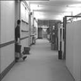
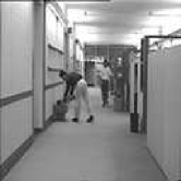
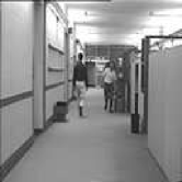
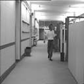
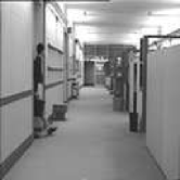
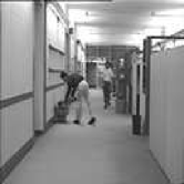
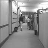
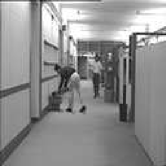
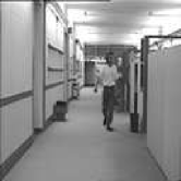
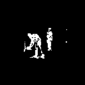
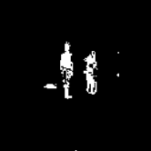
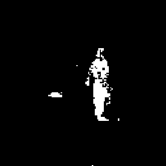
Figure 3: Hall sequence. The top panel shows the background and $4$ different frames of the original sequence, which consists of $282$ frames. The remaining panels show the estimated frames $e[k]$, the reconstructed frame $\hat{z}[k]$, and the reconstructed foreground $\hat{x}[k]$ (binarized for better visualization).

figures/VolkanAlg/HallCSmeasurements_oracle.dat figures/VolkanAlg/HallL1L1meas_oracle.dat figures/VolkanAlg/HallL1L1meas_estim.dat figures/VolkanAlg/HallMeasurements.dat

0.96

(a) Quantities related to the number of measurements.

figures/VolkanAlg/Hall_EstimError.dat figures/VolkanAlg/Hall_RecError.dat

0.96

(b) Relative errors of estimation and reconstruction.

Figure 4: Results for the Hall sequence. (a) Number of measurements $m_{k}$ taken from each frame (solid red line) and estimate $\phi_{k}$ (dashed blue line); the dotted lines are the right-hand side of (6) and (7) (green and black, respectively). (b) Relative error of estimation $\|e[k]-z[k]\|_{2}/\|z[k]\|_{2}$, and reconstruction $\|\hat{z}[k]-z[k]\|_{2}/\|z[k]\|_{2}$. Figure (b) is illustrative, since the reconstruction error is mostly determined by the precision of the solver for (4).

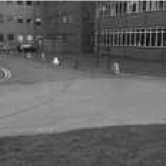
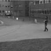
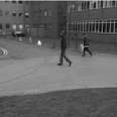
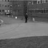
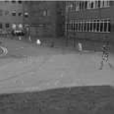
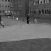
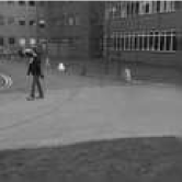
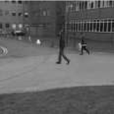
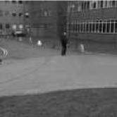
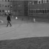
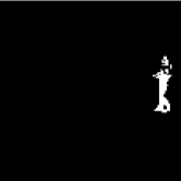
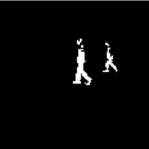
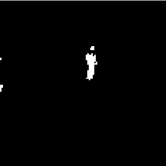
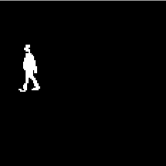
Figure 5: PETS sequence. The top panel shows the background and $4$ different frames of the original sequence, which consists of $171$ frames. The remaining panels show the estimated frames $e[k]$, the reconstructed frame $\hat{z}[k]$, and the reconstructed foreground $\hat{x}[k]$ (binarized for better visualization).

figures/VolkanAlg/PETSCSmeasurements_oracle.dat figures/VolkanAlg/PETSL1L1meas_oracle.dat figures/VolkanAlg/PETSL1L1meas_estim.dat figures/VolkanAlg/PETSMeasurements.dat

0.96

(a) Quantities related to the number of measurements.

figures/VolkanAlg/PETSEstimError.dat figures/VolkanAlg/PETSRecError.dat

0.96

(b) Relative errors of estimation and reconstruction.

Figure 6: Results for the PETS sequence. The displayed quantities are the same as in Fig. 4.

VI Experimental results

We applied the scheme described in the previous section to two sequences of images: the Hall monitor sequence and a sequence from the PETS 2009 database. The Hall monitor sequence has $282$ frames with two people walking in an office; the top panel of Fig. 3 shows the background image and frames $4$, $100$, $150$, and $250$. The PETS sequence is a sequence of $171$ frames with several people walking on a street; the top panel of Fig. 5 shows the background image and frames $5$, $75$, $100$, and $170$. Since the background of both sequences is static and the foreground in each frame is sparse, we can apply our scheme to simultaneously reconstruct and perform background subtraction on each frame. The remaining panels of Figs. 3 and 5 show the estimated frames, the reconstructed frames, and the reconstructed foregrounds, binarized for better visualization (note that the foreground pixels are dark).

Experimental setup. In both sequences, we set the oversampling parameters as $\delta:=\delta_{k}=0.1$, for all $k$, and the filter parameter as $\alpha=0.5$. While for the Hall sequence we used the true sparsity of the first two foregrounds, i.e., $\hat{s}_{1}=s_{1}=417$ and $\hat{s}_{2}=s_{2}=446$, for the PETS sequence we set these input parameters to values much smaller than their true values: $10=\hat{s}_{1}\ll s_{1}=194$ and $10=\hat{s}_{2}\ll s_{2}=211$. In spite of this poor initialization, the algorithm was able to quickly adapt, as we will see. For memory reasons, we downsampled each frame of the Hall sequence to $128\times 128$ and each frame of the PETS sequence to $116\times 116$. We also removed camera noise from each frame, i.e., isolated pixels, by preprocessing the full sequences. For the motion estimation, we used a block size of $\gamma\times\gamma=8\times 8$, and a search limit of $6$. Finally, we mention that, after computing the side information $w[k]$ for frame $k$, we amplified the magnitude of its components by $30\%$. This, according to the theory in [25], improves the quality of the side information. To solve basis pursuit in the reconstruction of the first two frames we used spgl1 [52, 53]. To solve $\ell_{1}$-$\ell_{1}$ minimization problem (4) in the reconstruction of the remaining frames we used decopt [54, 55].

Results. We benchmark Algorithm 1 with the CS (oracle) bound given by (7). Note that the prior state-of-the-art in compressive background subtraction, [21, 22], requires always more measurements than the ones given by (7). The results of the experiments are in Fig. 4 for the Hall sequence and in Fig. 6 for the PETS sequence. Figs. 4(a) and 6(a) show the number of measurements $m_{k}$ Algorithm 1 took from each frame and the corresponding estimate $\phi_{k}$ of (6). These figures also show the bounds (6) and (7) as if an oracle told us the true values of $s_{k}$, $\overline{h}_{k}$, and $\xi_{k}$. We can see that $m_{k}$ and $\phi_{k}$ are always below the CS bound (7), except at a few frames in Fig. 6(a) (PETS sequence). In those frames, there is no foreground and thus the number of required measurements approaches zero. Since there are no such frames in the Hall sequence, all quantities in Fig. 4(a) do not exhibit such large fluctuations. Fig. 4(a) clearly shows the advantage of our algorithm with respect to using standard CS (i.e., basis pursuit) [7, 21, 22], even if CS reconstruction is performed using the knowledge of the true foreground sparsity: our algorithm required an average of $33\%$ of the measurements that standard (oracle) CS required. Recall that the performance of the prior state-of-the-art algorithm [21, 22] is always above the CS bound line. In Figs. 4(a) and 6(a), the estimate $\phi_{k}$ is very close to the oracle bound (6) and, for most frames, the number of measurements $m_{k}$ is larger than (6), even though the oversampling factor $\delta=0.1$ is quite small. In fact, $m_{k}$ was smaller than (6) in less than $7\%$ (resp. $30\%$) of the frames for the Hall (resp. PETS) sequence. Yet, the corresponding frames were reconstructed with a relatively small error, as shown in Figs. 4(b) and 6(b), and the algorithm quickly adapted.

Figs. 4(b) and 6(b) show the relative errors of the estimated image $e[k]$ and the reconstruction image $\hat{z}[k]$, i.e., $\|e[k]-z[k]\|_{2}/\|z[k]\|_{2}$ and $\|\hat{z}[k]-z[k]\|_{2}/\|z[k]\|_{2}$. It can be seen that the estimation errors were approximately constant, around $0.01$ for the Hall sequence and around $0.93$ for the PETS sequence. The reconstruction error is essentially determined by the precision of the solver for (4). It varied between $3.8\times 10^{-9}$ and $3.5\times 10^{-6}$ for the Hall sequence [Fig. 4(b)]. For the PETS sequence [Fig. 6(b)], it was always below $10^{-5}$ except at three instances, where the reconstruction error approached the estimation error. These correspond to the frames with no foreground (making the bounds in (6) and (7) approach zero) and to the initial frames, where the number of measurements was much smaller than (6). In spite of these “ill-conditioned” frames, our algorithm was able to quickly adapt in the next frames, and follow the $\ell_{1}$-$\ell_{1}$ bound curve closely.

figures/noisy/HallCSmeasurements_oracle.dat figures/noisy/HallL1L1meas_oracle.dat figures/noisy/HallL1L1meas_estim.dat figures/noisy/HallMeasurements.dat

0.96

(a) Quantities related to the number of measurements.

figures/noisy/Hall_EstimError.dat figures/noisy/Hall_RecError.dat

0.96

(b) Relative errors of estimation and reconstruction.

Figure 7: Results for the Hall sequence for the noisy measurement case. The quantities are the same as in Fig. 4. The CS bound curve in (a) was truncated at $6000$ measurements so that the vertical scale is the same as in Fig. 4(a).

Noisy measurements. We also applied the version of Algorithm 1 that handles noisy measurements, i.e., $y[k]=A_{k}x[k]+\eta_{k}$, with $\|\eta_{k}\|_{2}\leq\sigma_{k}$, to the Hall sequence. In this case, $\eta_{k}$ was a vector of i.i.d. Gaussian entries with zero mean and variance $4/m_{k}$, and we used $\sigma_{k}=2$ for all frames. The number of measurements was computed as in (8) with $\tau=0.1$. The results are shown in Fig. 7. It can be seen that all the quantities in Fig. 7(a) are slightly larger than in Fig. 4(a) (we truncated the CS bound in Fig. 7(a) so that the vertical scales are the same). Yet, all the curves have the same shape. The most noticeable difference between the noisy and the noiseless case is the reconstruction error (Fig. 7(b)), which is about $3$ orders of magnitude larger for the noisy case.

VII Conclusions

We proposed and analyzed an online algorithm for reconstructing a sparse sequence of signals from a limited number of measurements. The signals vary across time according to a nonlinear dynamical model, and the measurements are linear. Our algorithm is based on $\ell_{1}$-$\ell_{1}$ minimization and, assuming Gaussian measurement matrices, it estimates the required number of measurements to perfectly reconstruct each signal, automatically and on-the-fly. We also explored the application of our algorithm to compressive video background subtraction and tested its performance on sequences of real images. It was shown that the proposed algorithm allows reducing the number of required measurements with respect to prior compressive video background subtraction schemes by a large margin.

Appendix A Proof of Lemma 2

First, note that condition (10) is a function only of the parameters of the sequences $\{x[k]\}$ and $\{\epsilon[k]\}$ and, therefore, is a deterministic condition. Simple algebraic manipulation shows that it is equivalent to

$$(1+\delta_{i})\bigg{[}2\overline{h}_{i-1}\log\Big{(}\frac{n}{u_{i-1}}\Big{)}+\frac{7}{5}u_{i-1}+1\bigg{]}\geq 2\overline{h}_{i}\log\Big{(}\frac{n}{u_{i}}\Big{)}\\ +\frac{7}{5}u_{i}+1\,,$$

or

$$(1+\delta_{i})\overline{m}_{i-1}\geq\overline{m}_{i}\,,$$ (20)

where $\overline{m}_{i}$ is the right-hand side of (6) applied to $x[i]$, that is,

$$\overline{m}_{i}:=2\overline{h}_{i}\log\Big{(}\frac{n}{s_{i}+\xi_{i}/2}\Big{)}+\frac{7}{5}\Big{(}s_{i}+\frac{\xi_{i}}{2}\Big{)}+1\,.$$ (21)

Notice that the source of randomness in Algorithm 1 is the set of matrices (random variables) $A_{k}$, generated in steps 6 and 17. Define the event $S_{i}$ as “perfect reconstruction at time $i$.” Since we assume that $\hat{s}_{1}$ and $\hat{s}_{2}$ are larger than the true sparsity of $x[1]$ and $x[2]$, there holds [42]

$$\mathbb{P}(S_{i})\geq 1-\exp\Big{[}-\frac{1}{2}(m_{i}-\sqrt{m_{i}})^{2}\Big{]}$$

$$\geq 1-\exp\Big{[}-\frac{1}{2}(\underline{m}-\sqrt{\underline{m}})^{2}\Big{]}\,,$$ (22)

for $i=1,2$, where the second inequality is due to $m_{i}\geq\underline{m}$ and $1-\exp(-(1/2)(x-\sqrt{x})^{2})$ being an increasing function.

Next, we compute the probability of the event “perfect reconstruction at time $i$” given that there was “perfect reconstruction at all previous time instants $l<i$,” i.e., $\mathbb{P}(S_{i}|\bigwedge_{l<i}S_{l})$, for all $i=3,\ldots,k$. Since we assume $\alpha=1$, we have $\phi_{i}=\hat{\overline{m}}_{i-1}$ and step 16 of Algorithm 1 becomes $m_{i}=(1+\delta_{i})\hat{\overline{m}}_{i-1}$, for all $i\geq 3$. Under the event $S_{i-1}$, i.e., $\hat{x}[i-1]=x[i-1]$, we have $\hat{\overline{h}}_{i-1}=\overline{h}_{i-1}$, $\hat{\xi}_{i-1}=\xi_{i-1}$, and $\hat{\overline{m}}_{i-1}=\overline{m}_{i-1}$, where $\overline{m}_{i-1}$ is defined in (21). (The hat variables are random variables.) Consequently, due to our assumption (20), step 16 can be written as $m_{i}=(1+\delta_{i})\hat{\overline{m}}_{i-1}=(1+\delta_{i})\overline{m}_{i-1}\geq\overline{m}_{i}$. This means (6) is satisfied and hence, for $i\geq 3$,

$$\mathbb{P}\Big{(}S_{i}\,\big{|}\,\bigwedge_{l<i}S_{l}\Big{)} \geq 1-\exp\Big{[}-\frac{1}{2}(m_{i}-\sqrt{m_{i}})^{2}\Big{]}$$

$$\geq 1-\exp\Big{[}-\frac{1}{2}(\underline{m}-\sqrt{\underline{m}})^{2}\Big{]}\,,$$ (23)

where, again, we used the fact that $m_{i}\geq\underline{m}$ and that $1-\exp(-(1/2)(x-\sqrt{x})^{2})$ is an increasing function.

Finally, we bound the probability that there is perfect reconstruction at all time instants $1\leq i\leq k$:

$$\mathbb{P}(S_{1} \wedge S_{2}\wedge\cdots\wedge S_{k})$$

$$=\mathbb{P}(S_{1})\mathbb{P}(S_{2}|S_{1})\prod_{i=3}^{k}\mathbb{P}(S_{i}|S_{1}\wedge\cdots\wedge S_{i-1})$$ (24)

$$=\mathbb{P}(S_{1})\mathbb{P}(S_{2})\prod_{i=3}^{k}\mathbb{P}\Big{(}S_{i}\,\big{|}\,\bigwedge_{l<i}S_{l}\Big{)}$$ (25)

$$\geq\bigg{(}1-\exp\Big{[}-\frac{1}{2}(\underline{m}-\sqrt{\underline{m}})^{2}\Big{]}\bigg{)}^{k}\,.$$ (26)

From (24) to (25) we used the independence between $S_{1}$ and $S_{2}$. From (25) to (26), we used (22) and (23). ∎

Appendix B Proof of Theorem 3

Recall the definitions of $\xi$ and $\overline{h}$ in (5):

$$\xi =\big{|}\{j\,:\,w_{j}\neq x_{j}^{\star}=0\}\big{|}-\big{|}\{j\,:\,w_{j}=x_{j}^{\star}\neq 0\}\big{|}$$

$$\overline{h} =\big{|}\{j\,:\,x_{j}^{\star}>0,\,\,\epsilon_{j}>0\}\cup\{j\,:\,x_{j}^{\star}<0,\epsilon_{j}<0\}\big{|}\,,$$

where we rewrote $\overline{h}$ using $x^{\star}=w+\epsilon$. Define the events $\mathcal{A}:=\text{``}\,\exists_{j}\,:\,x_{j}=w_{j}=0\,\text{''}$, $\mathcal{B}:=\text{``}\,\overline{h}>0\,\text{''}$, and

$$\mathcal{C}:=\text{``}\,m\geq 2\overline{h}\log\Big{(}\frac{n}{s+\xi/2}\Big{)}+\frac{7}{5}\Big{(}s+\frac{\xi}{2}\Big{)}+1\,\text{,''}$$

which are the assumptions of Theorem 1. In $\mathcal{C}$, $m$ and $n$ are deterministic, whereas $s$, $\overline{h}$, and $\xi$ are random variables. Then,

$$\mathbb{P}\big{(}\hat{x}=x^{\star}\big{)}\geq\mathbb{P}\Big{(}\hat{x}=x^{\star}\,\Big{|}\,\mathcal{A}\wedge\mathcal{B}\wedge\mathcal{C}\Big{)}\cdot\mathbb{P}\big{(}\mathcal{A}\wedge\mathcal{B}\wedge\mathcal{C}\big{)}$$

$$\geq\bigg{[}1-\exp\Big{(}-\frac{(m-\sqrt{m})^{2}}{2}\Big{)}\bigg{]}\cdot\mathbb{P}\big{(}\mathcal{A}\wedge\mathcal{B}\wedge\mathcal{C}\big{)}\,,$$ (27)

where we used Theorem 1. The rest of the proof consists of lower bounding $\mathbb{P}\big{(}\mathcal{A}\wedge\mathcal{B}\wedge\mathcal{C}\big{)}$.

Lower bound on $\mathbb{P}\big{(}\mathcal{A}\wedge\mathcal{B}\wedge\mathcal{C}\big{)}$. Recall that $w$ is fixed and that each component $x_{j}^{\star}$ is determined by $x_{j}^{\star}=w_{j}+\epsilon_{j}$. Due to the continuity of the distribution of $\epsilon$, with probability $1$, no component $j\in\Sigma$ (i.e., $\sigma_{j}^{2}\neq 0$) contributes to $\xi$. When $j\in\Sigma^{c}$, we have two cases:

• $j\in\Sigma^{c}\cap\mathcal{W}$ (i.e., $\sigma_{j}^{2}=0$ and $w_{j}\neq 0$): in this case, we have $x_{j}^{\star}=w_{j}$ with probability $1$. Hence, these components contribute to the second term of $\xi$.

• $j\in\Sigma^{c}\cap\mathcal{W}^{c}$ (i.e., $\sigma_{j}^{2}=0$ and $w_{j}=0$): in this case, we also have $x_{j}^{\star}=w_{j}$ with probability $1$. However, these components do not contribute to $\xi$.

We conclude $\mathbb{P}\big{(}\mathcal{D}\big{)}=\mathbb{P}\big{(}\xi=-\big{|}\Sigma^{c}\cap\mathcal{W}\big{|}\big{)}=1$, where $\mathcal{D}$ is the event “$\xi=-\big{|}\Sigma^{c}\cap\mathcal{W}\big{|}$.” From the second case above we also conclude that our assumption $\Sigma^{c}\cap\mathcal{W}^{c}\neq\emptyset$ implies $\mathbb{P}\big{(}\mathcal{A}\big{)}=1$. We can then write

$$\mathbb{P}\big{(}\mathcal{A}\wedge\mathcal{B}\wedge\mathcal{C}\big{)} =\mathbb{P}\big{(}\mathcal{A}\big{)}\cdot\mathbb{P}\big{(}\mathcal{B}\wedge\mathcal{C}\,\big{|}\,\mathcal{A}\big{)}=\mathbb{P}\big{(}\mathcal{B}\wedge\mathcal{C}\,\big{|}\,\mathcal{A}\big{)}$$

$$\geq\mathbb{P}\big{(}\mathcal{B}\wedge\mathcal{C}\,\big{|}\,\mathcal{A},\,\mathcal{D}\big{)}\cdot\mathbb{P}\big{(}\mathcal{D}\,\big{|}\,\mathcal{A}\big{)}$$ (28)

$$=\mathbb{P}\big{(}\mathcal{B}\wedge\mathcal{C}\,\big{|}\,\mathcal{A},\,\mathcal{D}\big{)}\cdot\mathbb{P}\big{(}\mathcal{D}\big{)}$$ (29)

$$=\mathbb{P}\big{(}\mathcal{B}\wedge\mathcal{C}\,\big{|}\,\mathcal{A},\,\mathcal{D}\big{)}$$ (30)

$$=\mathbb{P}\big{(}0<\overline{h}\leq\mu+t\,\big{|}\,\mathcal{A},\,\mathcal{D}\big{)}\,.$$ (31)

From (28) to (29), we used the fact that the events $\mathcal{A}=\text{``}\Sigma^{c}\cap\mathcal{W}^{c}\neq\emptyset\text{''}$ and $\mathcal{D}=\text{``}\xi=-|\Sigma^{c}\cap\mathcal{W}|\text{''}$ are independent. This follows from the independence of the components of $\epsilon$ and the disjointness of $\Sigma^{c}\cap\mathcal{W}^{c}$ and $\Sigma^{c}\cap\mathcal{W}$. From (30) to (31), we used the fact that event $\mathcal{C}$ conditioned on $\mathcal{D}$ is equivalent to $\overline{h}\leq\mu+t$. To see why, note that the sparsity of $x^{\star}$ is given by $s=|\Sigma|+|\Sigma^{c}\cap\mathcal{W}|$; thus, given $\mathcal{D}$, $s+\xi/2$ equals $|\Sigma|+|\Sigma^{c}\cap\mathcal{W}|/2$; now, subtract the expression in assumption (16) from the expression that defines event $\mathcal{C}$:

$$0\geq 2(\overline{h}-\mu-t)\log\bigg{[}\frac{n}{|\Sigma|+\frac{1}{2}|\Sigma^{c}\cap\mathcal{W}|}\bigg{]}\,.$$

Using the fact that $n=|\Sigma|+|\Sigma^{c}|\geq|\Sigma|+|\Sigma^{c}\cap\mathcal{W}|\geq|\Sigma|+|\Sigma^{c}\cap\mathcal{W}|/2$, we conclude that $\mathcal{C}$ is equivalent to the event “$\overline{h}\leq\mu+t$.” We now bound (31) as follows:

$$\mathbb{P}\big{(}0<\overline{h}\leq\mu+t\,\big{|}\,\mathcal{A},\,\mathcal{D}\big{)}$$

$$\geq\mathbb{P}\big{(}0<\overline{h}<\mu+t-1\,\big{|}\,\mathcal{A},\,\mathcal{D}\big{)}$$

$$=1-\mathbb{P}\big{(}\overline{h}\leq 0\,\big{|}\,\mathcal{A},\,\mathcal{D}\big{)}-\mathbb{P}\big{(}\overline{h}\geq\mu+t-1\,\big{|}\,\mathcal{A},\,\mathcal{D}\big{)}$$

$$=1-\mathbb{P}\big{(}\overline{h}-\mu\leq-\mu\,\big{|}\,\mathcal{A},\,\mathcal{D}\big{)}-\mathbb{P}\big{(}\overline{h}-\mu\geq t-1\,\big{|}\,\mathcal{A},\,\mathcal{D}\big{)}$$ (32)

$$\geq 1-\exp\bigg{[}-\frac{2\mu^{2}}{\big{|}\Sigma\big{|}}\bigg{]}-\exp\bigg{[}-\frac{2(t-1)^{2}}{\big{|}\Sigma\big{|}}\bigg{]}\,,$$ (33)

where the last step, explained below, is due to Hoeffding’s inequality [56]. Note that once this step is proven, (33) together with (27) and (31) give (17), proving the theorem.

Proof of step (32)-(33). Hoeffding’s inequality states that if $\{Z_{j}\}_{j=1}^{L}$ is a sequence of independent random variables and $\mathbb{P}(0\leq Z_{j}\leq 1)=1$ for all $j$, then [56, Th.4]:

$$\mathbb{P}\bigg{(}\sum_{j=1}^{L}Z_{j}-\sum_{j=1}^{L}\mathbb{E}\big{[}Z_{j}\big{]}\geq\tau\bigg{)} \leq\exp\Big{[}-\frac{2\tau^{2}}{L}\Big{]}$$ (34)

$$\mathbb{P}\bigg{(}\sum_{j=1}^{L}Z_{j}-\sum_{j=1}^{L}\mathbb{E}\big{[}Z_{j}\big{]}\leq-\tau\bigg{)} \leq\exp\Big{[}-\frac{2\tau^{2}}{L}\Big{]}\,,$$ (35)

for any $\tau>0$. We apply (35) to the second term in (32) and (34) to the third term. This is done by showing that $\overline{h}$ is the sum of $|\Sigma|$ independent random variables, taking values in $[0,1]$ with probability $1$, and whose expected values sum to $\mu$. Note that $\mu>0$ by definition, and $t>1$ by assumption.

We start by noticing that the components of $\epsilon$ that contribute to $\overline{h}$ are the ones for which $\sigma_{j}^{2}\neq 0$, i.e., $j\in\Sigma$ (otherwise, $\epsilon_{j}=0$ with probability $1$). Using the relation $x_{j}^{\star}=w_{j}+\epsilon_{j}$ [cf. (1a)], we then have $\overline{h}=\sum_{j\in\Sigma}Z_{j}$, where $Z_{j}$ is the indicator of the event

$$\epsilon_{j}>\max\big{\{}0,\,-w_{j}\big{\}}\quad\text{or}\quad\epsilon_{j}<\min\big{\{}0,\,-w_{j}\big{\}}\,,$$ (36)

that is, $Z_{j}=1$ if (36) holds, and $Z_{j}=0$ otherwise. By construction, $0\leq Z_{j}\leq 1$ for all $j$. Furthermore, because the components of $\epsilon$ are independent, so are the random variables $Z_{j}$. All we have left to do is to show that the sum of the expected values of $Z_{j}$ conditioned on $\mathcal{A}$ and $\mathcal{D}$ equals $\mu$. This involves just simple integration. Let $j\in\Sigma$. Then,

$$\mathbb{E}\Big{[}Z_{j}\,\big{|}\,\mathcal{A},\,\mathcal{D}\Big{]}=\mathbb{P}\big{(}Z_{j}=1\,\big{|}\,\mathcal{A},\,\mathcal{D}\big{)}$$ (37)

$$=\mathbb{P}\big{(}\epsilon_{j}>\max\big{\{}0,\,-w_{j}\big{\}}\big{)}+\mathbb{P}\big{(}\epsilon_{j}<\min\big{\{}0,\,-w_{j}\big{\}}\big{)}$$ (38)

$$=\frac{1+\exp\big{(}-\lambda_{j}\big{|}w_{j}\big{|}\big{)}}{2}$$ (39)

$$=\frac{1+\exp\big{(}-\sqrt{2}\big{|}w_{j}\big{|}/\sigma_{j}\big{)}}{2}\,.$$ (40)

From (37) to (38), we used the fact that the events in (36) are disjoint for any $w_{j}$. From (38) to (39), we used the fact that $\lambda_{j}$ is finite for $j\in\Sigma$, and

$$\mathbb{P}\big{(}\epsilon_{j}>\max\big{\{}0,\,-w_{j}\big{\}}\big{)} =\int_{\max\{-w_{j},0\}}^{+\infty}\frac{\lambda_{j}}{2}\exp(-\lambda_{j}|u|)\,du$$

$$=\left\{\begin{array}[]{ll}\frac{1}{2}&,\,\,w_{j}>0\vspace{0.3cm}\\ \frac{1}{2}\exp\big{(}\lambda_{j}w_{j}\big{)}&,\,\,w_{j}<0\end{array}\right.$$

$$\mathbb{P}\big{(}\epsilon_{j}<\min\big{\{}0,\,-w_{j}\big{\}}\big{)} =\int_{-\infty}^{\min\{-w_{j},0\}}\frac{\lambda_{j}}{2}\exp(\lambda_{j}|u|)\,du$$

$$=\left\{\begin{array}[]{ll}\frac{1}{2}\exp\big{(}-\lambda_{i}w_{j}\big{)}&,\,\,w_{j}>0\vspace{0.3cm}\\ \frac{1}{2}&,\,\,w_{j}<0\,.\end{array}\right.$$

And from (39) to (40) we simply replaced $\lambda_{j}=\sqrt{2}/\sigma_{j}$. The expected value of $\overline{h}$ conditioned on $\mathcal{A}$ and $\mathcal{D}$ is then

$$\mathbb{E}\Big{[}\overline{h}\,\big{|}\,\mathcal{A},\,\mathcal{D}\Big{]} =\mathbb{E}\Big{[}\sum_{j\in\Sigma}Z_{j}\,\big{|}\,\mathcal{A},\,\mathcal{D}\Big{]}=\sum_{j\in\Sigma}\mathbb{E}\Big{[}Z_{j}\,\big{|}\,\mathcal{A},\,\mathcal{D}\Big{]}$$

$$=\frac{1}{2}\sum_{j\in\Sigma}\Big{[}1+\exp\big{(}-\sqrt{2}\big{|}w_{j}\big{|}/\sigma_{j}\big{)}\Big{]}=:\mu\,,$$

where we used (40).

∎

References

• [1] J. Mota, N. Deligiannis, A. C. Sankaranarayanan, V. Cevher, and M. Rodrigues, “Dynamic sparse state estimation using $\ell_{1}$-$\ell_{1}$ minimization: Adaptive-rate measurement bounds, algorithms, and applications,” 2015, to appear in IEEE Intern. Conf. Acoustics, Speech, and Sig. Proc. (ICASSP).
• [2] D. A. Forsyth and J. Ponce, Computer Vision: A Modern Approach.   Prentice Hall, 2002.
• [3] R. Chellappa, A. C. Sankaranarayanan, A. Veeraraghavan, and P. Turaga, “Statistical methods and models for video-based tracking, modeling, and recognition,” Foundations and Trends in Signal Processing, vol. 3, no. 1-2, pp. 1–151, 2009.
• [4] M. Herman and T. Strohmer, “High-resolution radar via compressed sensing,” IEEE Trans. Sig. Proc., vol. 57, no. 6, pp. 2275–2284, 2009.
• [5] L. Weizman, Y. Eldar, and D. Bashat, “The application of compressed sensing for longitudinal MRI,” 2014, preprint: http://arxiv.org/abs/1407.2602.
• [6] A. Ribeiro, I. D. Schizas, S. I. Roumeliotis, and G. B. Giannakis, “Kalman filtering in wireless sensor networks,” IEEE Control Syst. Mag., vol. 30, no. 2, pp. 66–86, 2010.
• [7] V. Cevher, A. Sankaranarayanan, M. Duarte, D. Reddy, R. Baraniuk, and R. Chellappa, “Compressive sensing for background subtraction,” in European Conf. on Computer Vision (ECCV), 2008.
• [8] L. Maddalena and A. Petrosino, “A self-organizing approach to background subtraction for visual surveillance applications,” IEEE Trans. Image Processing, vol. 17, no. 7, pp. 1168–1177, 2008.
• [9] S. Brutzer, B. Höferlin, and G. Heidemann, “Evaluation of background subtraction techniques for video surveillance,” in IEEE Conf. Comp. Vision and Pattern Recognition (CVPR), 2011, pp. 1937–1944.
• [10] B. Tseng, C.-Y. Lin, and J. Smith, “Real-time video surveillance for traffic monitoring using virtual line analysis,” in IEEE Inter. Conf. Multimedia and Expo, 2002, pp. 541–544.
• [11] S. Cheung and C. Kamath, “Robust techniques for background subtraction in urban traffic video,” in Symposium on Electronic Imaging (SPIE), 2003, pp. 881–892.
• [12] A. Profio, O. Balchum, and F. Carstens, “Digital background subtraction for fluorescence imaging,” Med. Phys., vol. 13, no. 5, pp. 717–721, 1986.
• [13] R. Otazo, E. Candès, and D. Sodickson, “Low-rank plus sparse matrix decomposition for accelerated dynamic MRI with separation of background and dynamic components,” 2014, to appear in Magnetic Resonance in Medicine.
• [14] M. Piccardi, “Background subtraction techniques: a review,” in IEEE Inter. Conf. Systems, Man and Cybernetics, 2004, pp. 3099–3104.
• [15] E. Candès, X. Li, Y. Ma, and J. Wright, “Robust principal component analysis?” Journal of the ACM, vol. 58, no. 3, pp. 11:1–11:37, 2011.
• [16] M. Wakin, J. Laska, M. Duarte, D. Baron, S. Sarvotham, D. Takhar, K. Kelly, and R. Baraniuk, “Compressive imaging for video representation and coding,” in Picture Coding Symposium, 2006.
• [17] A. Sankaranarayanan, C. Studer, and R. Baraniuk, “CS-MUVI: video compressive sensing for spatial multiplexing cameras,” in Intern. Conf. Computation Photography, 2012, pp. 1–10.
• [18] A. Sankaranarayanan, P. Turaga, R. Chellapa, and R. Baranuik, “Compressive acquisition of linear dynamical systems,” SIAM J. Imaging Sciences, vol. 6, no. 4, pp. 2109–2133, 2013.
• [19] D. Donoho, “Compressed sensing,” IEEE Trans. Inf. Th., vol. 52, no. 4, pp. 1289–1306, 2006.
• [20] E. Candès, J. Romberg, and T. Tao, “Robust uncertainty principles: Exact signal reconstruction from highly incomplete frequency information,” IEEE Trans. Inf. Th., vol. 52, no. 2, pp. 489–509, 2006.
• [21] G. Warnell, D. Reddy, and R. Chellappa, “Adaptive rate compressive sensing for background subtraction,” in IEEE Intern. Conf. Acoustics, Speech, and Sig. Proc. (ICASSP), 2012, pp. 1477–1480.
• [22] G. Warnell, S. Bhattacharya, R. Chellappa, and T. Basar, “Adaptive-rate compressive sensing using side information,” 2014, preprint: http://arxiv.org/abs/1401.0583.
• [23] J. Park and M. Wakin, “A multiscale framework for compressive sensing of video,” in Picture Coding Symposium, 2009, pp. 1–4.
• [24] D. Reddy, A. Veeraraghavan, and R. Chellappa, “P2C2: programmable pixel compressive camera for high speed imaging,” in IEEE Conf. Comp. Vision and Pattern Recognition (CVPR), 2011, pp. 329–336.
• [25] J. Mota, N. Deligiannis, and M. Rodrigues, “Compressed sensing with prior information: Optimal strategies, geometry, and bounds,” 2014, preprint: http://arxiv.org/abs/1408.5250.
• [26] ——, “Compressed sensing with side information: Geometrical interpretation and performance bounds,” in IEEE Global Conf. Sig. and Inf. Proc. (GlobalSIP), 2014, pp. 675–679.
• [27] S. Chen, D. Donoho, and M. Saunders, “Atomic decomposition by basis pursuit,” SIAM J. Sci. Comp., vol. 20, no. 1, pp. 33–61, 1998.
• [28] R. Berinde and P. Indyk, “Sparse recovery using sparse matrices,” MIT-CSAIL-TR-2008-001, Tech. Rep., 2008.
• [29] A. Liutkis, D. Martina, S. Popoff, G. Chardon, O. Katz, G. Lerosey, S. Gigan, L. Daudet, and I. Carron, “Imaging with nature: Compressive imaging using a multiply scattering medium,” Nature, vol. 4, no. 5552, pp. 1–7, 2014.
• [30] R. Kalman, “A new approach to linear filtering and prediction problems,” Trans. ASME-J. Basic Engineering, vol. 82, no. D, pp. 35–45, 1960.
• [31] S. Haykin, Kalman Filtering and Neural Networks.   John Wiley and Sons, 2001.
• [32] J. Geromel, “Optimal linear filtering under parameter uncertainty,” IEEE Trans. Sig. Proc., vol. 47, no. 1, pp. 168–175, 1999.
• [33] L. El Ghaoui and G. Calafiore, “Robust filtering for discrete-time systems with bounded noise and parametric uncertainty,” IEEE Trans. Autom. Control, vol. 46, no. 7, pp. 1084–1089, 2001.
• [34] N. Vaswani, “Kalman filtered compressed sensing,” in IEEE Intern. Conf. Image Processing (ICIP), 2008, pp. 893–896.
• [35] ——, “Analyzing least squares and Kalman filtered compressed sensing,” in IEEE Intern. Conf. Acoustics, Speech, and Sig. Proc. (ICASSP), 2009, pp. 3013–3016.
• [36] J. Ziniel, L. Potter, and P. Schniter, “Tracking and smoothing of time-varying sparse signals via approximate belief propagation,” in Asilomar Conf. Signals, Systems, and Computers, 2010, pp. 808–812.
• [37] A. Carmi, P. Gurfil, and D. Kanevsky, “Methods for sparse signal recovery using Kalman filtering with embedded pseudo-measurement norms and quasi-norms,” IEEE Trans. Sig. Proc., vol. 58, no. 4, pp. 2405–2409, 2010.
• [38] L. Balzano, R. Nowak, and B. Recht, “Online identification and tracking of subspaces from highly incomplete information,” in Allerton Conf. Communications, Control, and Computing, 2010, pp. 704–711.
• [39] L. Balzano and S. J. Wright, “Local convergence of an algorithm for subspace identification from partial data,” Found. Computational Mathematics, pp. 1–36, 2014.
• [40] Y. Chi, Y. C. Eldar, and R. Calderbank, “PETRELS: Parallel subspace estimation and tracking by recursive least squares from partial observations,” IEEE Trans. Sig. Proc., vol. 61, no. 23, pp. 5947–5959, 2013.
• [41] A. Charles, M. Asif, J. Romberg, and C. Rozell, “Sparsity penalties in dynamical system estimation,” in IEEE Conf. Information Sciences and Systems, 2011, pp. 1–6.
• [42] V. Chandrasekaran, B. Recht, P. Parrilo, and A. Willsky, “The convex geometry of linear inverse problems,” Found. Computational Mathematics, vol. 12, pp. 805–849, 2012.
• [43] M. Duarte, M. Davenport, D. Takhar, J. Laska, T. Sun, K. Kelly, and R. Baraniuk, “Single-pixel imaging via compressive sampling,” IEEE Sig. Proc. Mag., vol. 25, no. 2, pp. 83–91, 2008.
• [44] D. Kanevsky, A. Carmi, L. Horesh, P. Gurfil, B. Ramabhadran, and T. Sainath, “Kalman filtering for compressed sensing,” in Conf. Information Fusion (FUSION), 2010, pp. 1–8.
• [45] B. Girod, A. Aaron, S. Rane, and D. Rebollo-Monedero, “Distributed video coding,” Proc. IEEE, vol. 93, no. 1, pp. 71–83, 2005.
• [46] N. Deligiannis, J. Barbarien, M. Jacobs, A. Munteanu, A. Skodras, and P. Schelkens, “Side-information-dependent correlation channel estimation in hash-based distributed video coding,” IEEE Trans. Image Processing, vol. 21, no. 4, pp. 1934–1949, 2012.
• [47] L. Natário, C. Brites, J. Ascenso, and F. Pereira, “Extrapolating side information for low-delay pixel-domain distributed video coding,” in Visual Content Processing and Representation, 2006, pp. 16–21.
• [48] T. Wiegand, G. J. Sullivan, G. Bjontegaard, and A. Luthra, “Overview of the H. 264/AVC video coding standard,” IEEE Trans. Circuits Sys. for Video Tech., vol. 13, no. 7, pp. 560–576, 2003.
• [49] L. Alparone, M. Barni, F. Bartolini, and V. Cappellini, “Adaptively weighted vector-median filters for motion-fields smoothing,” in IEEE Intern. Conf. Acoustics, Speech, and Sig. Proc. (ICASSP), 1996, pp. 2267–2270.
• [50] N. Deligiannis, A. Munteanu, S. Wang, S. Cheng, and P. Schelkens, “Maximum likelihood Laplacian correlation channel estimation in layered Wyner-Ziv coding,” IEEE Trans. Sig. Proc., vol. 62, no. 4, pp. 892–904, 2014.
• [51] X. Fan, O. C. Au, and N. M. Cheung, “Transform-domain adaptive correlation estimation (TRACE) for Wyner-Ziv video coding,” IEEE Trans. Circuits Sys. for Video Tech., vol. 20, no. 11, pp. 1423–1436, 2010.
• [52] E. van den Berg and M. Friedlander, “Probing the Pareto frontier for basis pursuit solutions,” SIAM J. Sci. Comput., vol. 31, no. 2, pp. 890–912, 2008.
• [53] ——, “Sparse optimization with least-squares constraints,” SIAM J. Optim., vol. 21, no. 4, pp. 1201–1229, 2011.
• [54] Q. Tran-Dinh and V. Cevher, “Constrained convex minimization via model-based excessive gap,” in Proceedings of Neural Information Processing Systems Foundation (NIPS), 2014.
• [55] ——, “A primal-dual algorithmic framework for constrained convex minimization,” 2014, preprint: http://arxiv.org/abs/1406.5403.
• [56] G. Lugosi, “Concentration-of-measure inequalities,” 2009, lecture notes.