Relativistic quantum transport coefficients for second-order viscous hydrodynamics

Abstract

We express the transport coefficients appearing in the second-order evolution equations for bulk viscous pressure and shear stress tensor using Bose-Einstein, Boltzmann, and Fermi-Dirac statistics for the equilibrium distribution function and Grad’s 14-moment approximation as well as the method of Chapman-Enskog expansion for the non-equilibrium part. Specializing to the case of transversally homogeneous and boost-invariant longitudinal expansion of the viscous medium, we compare the results obtained using the above methods with those obtained from the exact solution of the massive 0+1d relativistic Boltzmann equation in the relaxation-time approximation. We show that compared to the 14-moment approximation, the hydrodynamic transport coefficients obtained by employing the Chapman-Enskog method leads to better agreement with the exact solution of the relativistic Boltzmann equation.

I Introduction

Relativistic viscous hydrodynamics has been applied quite successfully to study and understand various collective phenomena observed in the evolution of the strongly interacting QCD matter, with very high temperature and density, created in relativistic heavy-ion collisions; see Ref. Heinz:2013th for a recent review. The derivation of hydrodynamic equations is essentially a coarse graining procedure whereby one obtains an effective theory describing the long-wavelength low-frequency limit of the microscopic dynamics of a system Heinz:2013th ; Landau . Relativistic hydrodynamics is formulated as an order-by-order expansion in powers of space-time gradients where ideal hydrodynamics is of zeroth order Heinz:2013th . The viscous effects arising in the first-order theory, also known as the relativistic Navier-Stokes theory Eckart:1940zz ; Landau , results in acausal signal propagation and numerical instability. While causality is restored in the second-order Israel-Stewart (IS) theory Israel:1979wp , stability may not be guaranteed Romatschke:2009im . Consistent formulation of a causal theory of relativistic viscous hydrodynamics and accurate determination of the associated transport coefficients is currently an active research topic Muronga:2003ta ; El:2009vj ; Denicol:2012cn ; Jaiswal:2014isa ; Chattopadhyay:2014lya ; Denicol:2010xn ; Jaiswal:2012qm ; Jaiswal:2013fc ; Bhalerao:2013aha ; Denicol:2014vaa ; Denicol:2014mca ; Jaiswal:2013npa ; Jaiswal:2013vta ; Bhalerao:2013pza ; Romatschke:2003ms ; Florkowski:2010cf ; Martinez:2010sc ; Florkowski:2013lza ; Bazow:2013ifa ; Nopoush:2014pfa ; Florkowski:2014bba ; Florkowski:2014sfa ; Florkowski:2014sda ; Prakash:1993bt ; Wiranata:2012br ; Wiranata:2012vv ; Davesne:1995ms ; Wiranata:2014jda .

The second-order IS equations can be derived in several ways Romatschke:2009im . For example, in the derivations based on the second law of thermodynamics, the hydrodynamic transport coefficients related to the relaxation times for bulk and shear viscous evolution remain undetermined. While these transport coefficients can be obtained in the derivations based on kinetic theory Israel:1979wp ; Muronga:2003ta , the form of non-equilibrium phase-space distribution function, $f(x,p)$, has to be specified. Two most extensively used methods to determine $f(x,p)$ for a system which is close to local thermodynamic equilibrium are (1) the Grad’s 14-moment approximation Grad and (2) the Chapman-Enskog method Chapman . Note that while Grad’s 14-moment approximation has been widely employed in the formulation of a causal theory of relativistic dissipative hydrodynamics Israel:1979wp ; Muronga:2003ta ; El:2009vj ; Denicol:2010xn ; Denicol:2012cn ; Jaiswal:2012qm ; Jaiswal:2013fc ; Bhalerao:2013aha ; Denicol:2014vaa ; Denicol:2014mca ; Romatschke:2009im , the Chapman-Enskog method remains less explored Jaiswal:2013npa ; Jaiswal:2013vta ; Bhalerao:2013pza ; Jaiswal:2014isa ; Chattopadhyay:2014lya . On the other hand, the Chapman-Enskog formalism has been often used to extract various transport coefficients of hot hadronic matter Prakash:1993bt ; Wiranata:2012br ; Wiranata:2012vv ; Davesne:1995ms ; Wiranata:2014jda Although in both methods the distribution function is expanded around its equilibrium value $f_{0}(x,p)$, it has been demonstrated that the Chapman-Enskog method in the relaxation-time approximation (RTA) leads to better agreement with both microscopic Boltzmann simulations as well as exact solutions of the relativistic RTA Boltzmann equation Jaiswal:2013npa ; Jaiswal:2013vta ; Jaiswal:2014isa ; Chattopadhyay:2014lya . This may be attributed to the fact that a fixed-order moment expansion, as required in Grad’s approximation, is not necessary in the Chapman-Enskog method.

Much of the research on the application of viscous hydrodynamics in relativistic heavy-ion collisions is devoted to the extraction of the shear viscosity to entropy density ratio, $\eta/s$, from the analysis of the anisotropic flow data Romatschke:2007mq ; Song:2010mg ; Schenke:2011bn . Indeed the estimated $\eta/s$ has been found to be close to the conjectured lower bound $\eta/s|_{\rm KSS}=1/4\pi$ Policastro:2001yc ; Kovtun:2004de . On the other hand, a self-consistent and systematic study of the effect of the bulk viscosity in numerical simulations of high-energy heavy-ion collisions is relatively lacking. This may be attributed to the fact that the hot QCD matter is assumed to be nearly conformal and therefore the bulk viscosity is estimated to be much smaller compared to the shear viscosity. However, in reality, QCD is a non-conformal field theory and therefore bulk viscous corrections to the energy-momentum tensor should not be ignored in order to correctly understand the dynamics of the QCD system. Moreover, for the range of temperature explored in heavy-ion collision experiments at Relativistic Heavy-Ion Collider (RHIC) and Large Hadron Collider (LHC), the magnitude and temperature dependence of the bulk viscosity could be large enough to influence the space-time evolution of the hot QCD matter Moore:2008ws ; Noronha-Hostler:2014dqa ; Rose:2014fba ; Ryu:2015vwa ; Wiranata:2009cz ; Gavin:1985ph ; Chakraborty:2010fr .

It is important to note that the second-order transport coefficients, appearing in the evolution equation for the bulk viscous pressure, are less understood compared to those of the shear stress tensor. While the relaxation time for the bulk viscous evolution can be obtained by using the second law of thermodynamics in a kinetic theory set up Jaiswal:2013fc ; Bhalerao:2013aha , this method fails to account for the important coupling of the bulk viscous pressure with the shear stress tensor Denicol:2014vaa ; Denicol:2014mca ; Jaiswal:2014isa . On the other hand, for finite masses and classical Boltzmann distribution, the second-order transport coefficients corresponding to bulk viscous pressure and shear stress tensor have been obtained by employing the Grad’s 14-moment approximation Denicol:2014vaa ; Denicol:2014mca as well as the Chapman-Enskog method Jaiswal:2014isa , within a purely kinetic theory framework. However, these transport coefficients still remain to be determined for quantum statistics, i.e., for Bose-Einstein and Fermi-Dirac distribution.

In this paper, we express the transport coefficients appearing in the second-order viscous evolution equations with non-vanishing masses for Bose-Einstein, Boltzmann and Fermi-Dirac distribution. We obtain these transport coefficients using the Grad’s 14-moment approximation as well as the method of Chapman-Enskog expansion. In addition, in the case of one-dimensional scaling expansion of the viscous medium, we compare the results obtained using the above methods with those obtained from the exact solution of massive 0+1d relativistic Boltzmann equation in the relaxation-time approximation Florkowski:2014sda . We demonstrate that the results obtained using the Chapman-Enskog method are in better agreement with the exact solution of the RTA Boltzmann equation than those obtained using the Grad’s 14-moment approximation.

II Relativistic hydrodynamics

In the absence of any conserved charges, i.e., for vanishing chemical potential, the hydrodynamic evolution of a system is governed by the local conservation of energy and momentum: $\partial_{\mu}T^{\mu\nu}=0$. The energy-momentum tensor, $T^{\mu\nu}$, which characterizes the macroscopic state of a system, can be expressed in terms of the single-particle phase-space distribution function, $f(x,p)$, and tensor decomposed into hydrodynamic degrees of freedom deGroot ,

$$T^{\mu\nu}=\!\int\!dP\,p^{\mu}p^{\nu}f(x,p)=\epsilon u^{\mu}u^{\nu}-(P+\Pi)\Delta^{\mu\nu}+\pi^{\mu\nu}.$$ (1)

Here $dP\equiv gd^{3}p/[(2\pi)^{3}p^{0}]$ is the invariant momentum-space integration measure, $g$ being the degeneracy factor, and $p^{\mu}$ is the particle four-momentum. In the tensor decomposition, $\epsilon$, $P$, $\Pi$, and $\pi^{\mu\nu}$ are the energy density, the thermodynamic pressure, the bulk viscous pressure, and the shear stress tensor, respectively. The projection operator $\Delta^{\mu\nu}\equiv g^{\mu\nu}-u^{\mu}u^{\nu}$ is constructed such that it is orthogonal to the hydrodynamic four-velocity $u^{\mu}$. The metric tensor is assumed to be Minkowskian, $g^{\mu\nu}\equiv\mathrm{diag}({+}1,{-}1,{-}1,{-}1)$, and $u^{\mu}$ is defined in the Landau frame: $T^{\mu\nu}u_{\nu}=\epsilon u^{\mu}$.

The energy-momentum conservation equation, $\partial_{\mu}T^{\mu\nu}=0$, when projected along and orthogonal to $u^{\mu}$ gives the evolution equations for $\epsilon$ and $u^{\mu}$,

$$\dot{\epsilon}+(\epsilon+P+\Pi)\theta-\pi^{\mu\nu}\sigma_{\mu\nu} =0,$$

$$(\epsilon+P+\Pi)\dot{u}^{\alpha}-\nabla^{\alpha}(P+\Pi)+\Delta^{\alpha}_{\nu}\partial_{\mu}\pi^{\mu\nu} =0.$$ (2)

Here we have used the usual notation $\theta\equiv\partial_{\mu}u^{\mu}$ for the expansion scalar, $\dot{A}\equiv u^{\mu}\partial_{\mu}A$ for the co-moving derivative, $\nabla^{\alpha}\equiv\Delta^{\mu\alpha}\partial_{\mu}$ for the space-like derivative, and $\sigma^{\mu\nu}\equiv(\nabla^{\mu}u^{\nu}+\nabla^{\nu}u^{\mu})/2-(\theta/3)\Delta^{\mu\nu}$ for the velocity stress tensor. The energy density and the thermodynamic pressure can be written in terms of the equilibrium phase-space distribution function $f_{0}$ as

$$\epsilon_{0} =u_{\mu}u_{\nu}\!\int\!dP\,p^{\mu}p^{\nu}f_{0},$$ (3)

$$P_{0} =-\frac{1}{3}\Delta_{\mu\nu}\!\int\!dP\,p^{\mu}p^{\nu}f_{0},$$ (4)

where the equilibrium distribution function for vanishing chemical potential is given by

$$f_{0}=\frac{1}{\exp(\beta u\cdot p)+a}.$$ (5)

Here $u\cdot p\equiv u_{\mu}p^{\mu}$ and $a=-1,0,1$ for Bose-Einstein, Boltzmann, and Fermi-Dirac gas, respectively. The inverse temperature, $\beta\equiv 1/T$, is determined by the matching condition $\epsilon=\epsilon_{0}$.

For a system close to local thermodynamic equilibrium, the non-equilibrium phase-space distribution function can be written as $f=f_{0}+\delta f$, where $\delta f\ll f$. Using Eq. (1), the bulk viscous pressure, $\Pi$, and the shear stress tensor, $\pi^{\mu\nu}$, can be expressed in terms of $\delta f$ as deGroot

$$\Pi =-\frac{1}{3}\Delta_{\alpha\beta}\!\int\!dP\,p^{\alpha}p^{\beta}\,\delta f,$$ (6)

$$\pi^{\mu\nu} =\Delta^{\mu\nu}_{\alpha\beta}\!\int\!dP\,p^{\alpha}p^{\beta}\,\delta f,$$ (7)

where $\Delta^{\mu\nu}_{\alpha\beta}\equiv(\Delta^{\mu}_{\alpha}\Delta^{\nu}_{\beta}+\Delta^{\mu}_{\beta}\Delta^{\nu}_{\alpha})/2-(1/3)\Delta^{\mu\nu}\Delta_{\alpha\beta}$ is a traceless symmetric projection operator orthogonal to $u^{\mu}$ and $\Delta^{\mu\nu}$. In the following, we employ the expressions for $\delta f$ obtained using the Grad’s 14-moment approximation and the Chapman-Enskog like iterative solution of the relativistic Boltzmann equation to obtain expressions for the quantum transport coefficients associated with viscous evolution.

III Viscous corrections to the distribution function

Precise determination of the form of the non-equilibrium single particle phase-space distribution function is one of the central problems in statistical physics. For a system close to local thermodynamic equilibrium, the problem reduces to determining the form of the correction to the equilibrium distribution function. Within the framework of relativistic hydrodynamics, the viscous corrections to the equilibrium distribution function can be obtained from two different methods: (1) the moment method and (2) the Chapman-Enskog method. The moment method, more popularly known as the Grad’s 14-moment ansatz, is based on a Taylor-like expansion of the non-equilibrium distribution in powers of momenta. On the other hand, the Chapman-Enskog method relies on the solution of the Boltzmann equation.

Ignoring dissipation due to particle diffusion, the Grad’s 14-moment approximation leads to

$$\delta f_{\rm G}=\, \Big{[}\left\{E_{0}+B_{0}m^{2}+D_{0}(u\cdot p)-4B_{0}(u\cdot p)^{2}\right\}\Pi$$

$$+B_{2}p^{\alpha}p^{\beta}\pi_{\alpha\beta}\Big{]}f_{0}\tilde{f}_{0},$$ (8)

where $\tilde{f}_{0}=1-af_{0}$. The coefficients $E_{0}$, $B_{0}$, $D_{0}$ and $B_{2}$ are known in terms of $m$, $T$ and $u\cdot p$ and can be expressed as

$$B_{2}=\, \frac{1}{2J^{(0)}_{42}},$$ (9)

$$\frac{D_{0}}{3B_{0}}=\, 4\frac{J^{(0)}_{31}J^{(0)}_{20}-J^{(0)}_{41}J^{(0)}_{10}}{J^{(0)}_{30}J^{(0)}_{10}-J^{(0)}_{20}J^{(0)}_{20}}\equiv C_{2},$$ (10)

$$\frac{E_{0}}{3B_{0}}=\; m^{2}-4\frac{J^{(0)}_{31}J^{(0)}_{30}-J^{(0)}_{41}J^{(0)}_{20}}{J^{(0)}_{30}J^{(0)}_{10}-J^{(0)}_{20}J^{(0)}_{20}}\equiv C_{1},$$ (11)

$$B_{0}=\, -\frac{1}{3C_{1}J^{(0)}_{21}+3C_{2}J^{(0)}_{31}-3J^{(0)}_{41}+5J^{(0)}_{42}},$$ (12)

where the thermodynamic functions $J^{(r)}_{nq}$ are defined as

$$J_{nq}^{(r)}\equiv\frac{1}{(2q+1)!!}\!\int\!dP\,(u\cdot p)^{n-2q-r}\,(\Delta_{\mu\nu}p^{\mu}p^{\nu})^{q}f_{0}\tilde{f}_{0}.$$ (13)

In the above equation, the indices $n-r$ and $q$ represents the number of times $p^{\mu}$ and $\Delta_{\mu\nu}$ appear in the integration, respectively.

An analogous expression for $\delta f$ can also be obtained using an iterative Chapman-Enskog like solution of the relativistic Boltzmann equation in the relaxation-time approximation Romatschke:2011qp ; Jaiswal:2014isa . In absence of dissipation due to particle diffusion, the Chapman-Enskog method leads to Jaiswal:2014isa

$$\delta f_{\rm CE}=\frac{\beta}{u\cdot p}\bigg{[} -\frac{1}{3\beta_{\Pi}}\left\{m^{2}-(1-3c_{s}^{2})(u\cdot p)^{2}\right\}\Pi$$

$$+\frac{1}{2\beta_{\pi}}\;p^{\mu}p^{\nu}\pi_{\mu\nu}\bigg{]}f_{0}\tilde{f}_{0},$$ (14)

where

$$\beta_{\Pi} =\frac{5}{3}\beta_{\pi}-(\epsilon+P)c_{s}^{2},$$ (15)

$$\beta_{\pi} =\beta\,J_{42}^{(1)},$$ (16)

and $c_{s}^{2}\equiv dP/d\epsilon$ is the speed of sound squared which can be expressed as

$$c_{s}^{2}=\frac{\epsilon+P}{\beta J_{30}^{(0)}}.$$ (17)

IV Viscous evolution equations

The second-order evolution equations for $\Pi$ and $\pi^{\mu\nu}$ can be derived by considering the co-moving derivative of Eqs. (6) and (7),

$$\dot{\Pi} =-\frac{1}{3}\Delta_{\alpha\beta}\!\int\!dP\,p^{\alpha}p^{\beta}\,\delta\dot{f},$$ (18)

$$\dot{\pi}^{\langle\mu\nu\rangle} =\Delta^{\mu\nu}_{\alpha\beta}\!\int\!dP\,p^{\alpha}p^{\beta}\,\delta\dot{f}.$$ (19)

Further, $\delta\dot{f}$ appearing in the above equations can be simplified by rewriting the relativistic Boltzmann equation,

$$p^{\mu}\partial_{\mu}f=C[f],$$ (20)

in the form Denicol:2010xn

$$\delta\dot{f}=-\dot{f}_{0}-\frac{1}{u\cdot p}\,p^{\mu}\nabla_{\mu}f+\frac{1}{u\cdot p}\,C[f].$$ (21)

In the following, we consider the relaxation-time approximation for the collision term in the Boltzmann equation,

$$C[f]=-\left(u\cdot p\right)\frac{\delta f}{\tau_{\rm eq}},$$ (22)

where $\tau_{\rm eq}$ is the relaxation time. In general, in order for the collision term in the above equation to respect the conservation of particle four-current and energy-momentum tensor, $\tau_{\rm eq}$ must be independent of momenta and $u^{\mu}$ has to be defined in the Landau frame Anderson_Witting .

Substituting $\delta\dot{f}$ from Eq. (21) into Eqs. (18) and (19) along with the form of $\delta f$ given in Eqs. (III) and (III), and after performing the integrations, we obtain

$$\dot{\Pi}= -\frac{\Pi}{\tau_{\rm eq}}-\beta_{\Pi}\theta-\delta_{\Pi\Pi}\Pi\theta+\lambda_{\Pi\pi}\pi^{\mu\nu}\sigma_{\mu\nu},$$ (23)

$$\dot{\pi}^{\langle\mu\nu\rangle}= -\frac{\pi^{\mu\nu}}{\tau_{\rm eq}}+2\beta_{\pi}\sigma^{\mu\nu}+2\pi_{\gamma}^{\langle\mu}\omega^{\nu\rangle\gamma}-\delta_{\pi\pi}\pi^{\mu\nu}\theta$$

$$-\tau_{\pi\pi}\pi_{\gamma}^{\langle\mu}\sigma^{\nu\rangle\gamma}+\lambda_{\pi\Pi}\Pi\sigma^{\mu\nu},$$ (24)

where $\omega^{\mu\nu}\equiv\frac{1}{2}(\nabla^{\mu}u^{\nu}-\nabla^{\nu}u^{\mu})$ is the vorticity tensor. Note that the above form of the evolution equations for the bulk viscous pressure and the shear stress tensor is exactly same for both Grad’s 14-moment approximation ($\delta f_{G}$) and the Chapman-Enskog expansion ($\delta f_{CE}$). Moreover, the expressions for the first order transport coefficients, $\beta_{\Pi}$ and $\beta_{\pi}$, are also identical for these two cases and are given in Eqs. (15) and (16). However, the second order transport coefficients appearing in the above equations are different for the Grad’s 14-moment method and the Chapman-Enskog method.

The transport coefficients in the case of Grad’s 14-moment approximation are calculated to be

$$\delta^{\rm(G)}_{\Pi\Pi} =1-c_{s}^{2}-\frac{m^{4}}{9}\gamma^{(0)}_{2},$$ (25)

$$\lambda^{\rm(G)}_{\Pi\pi} =\frac{1}{3}-c_{s}^{2}+\frac{m^{2}}{3}\gamma^{(2)}_{2},$$ (26)

$$\delta^{\rm(G)}_{\pi\pi} =\frac{4}{3}+\frac{m^{2}}{3}\gamma^{(2)}_{2},$$ (27)

$$\tau^{\rm(G)}_{\pi\pi} =\frac{10}{7}+\frac{4m^{2}}{7}\gamma^{(2)}_{2},$$ (28)

$$\lambda^{\rm(G)}_{\pi\Pi} =\frac{6}{5}-\frac{2m^{4}}{15}\gamma^{(0)}_{2},$$ (29)

where

$$\gamma^{(0)}_{2} =(E_{0}+B_{0}m^{2})J^{(0)}_{-20}+D_{0}J^{(0)}_{-10}-4B_{0}J^{(0)}_{00},$$ (30)

$$\gamma^{(2)}_{2} =\frac{J^{(0)}_{22}}{J^{(0)}_{42}}.$$ (31)

On the other hand, these transport coefficients in the case of Chapman-Enskog method are obtained as

$$\delta^{\rm(CE)}_{\Pi\Pi} =-\frac{5}{9}\,\chi-c_{s}^{2},$$ (32)

$$\lambda^{\rm(CE)}_{\Pi\pi} =\frac{\beta}{3\beta_{\pi}}\!\left(7J_{63}^{(3)}+2J_{42}^{(1)}\right)-c_{s}^{2},$$ (33)

$$\delta^{\rm(CE)}_{\pi\pi} =\frac{5}{3}+\frac{7\beta}{3\beta_{\pi}}\,J_{63}^{(3)},$$ (34)

$$\tau^{\rm(CE)}_{\pi\pi} =2+\frac{4\beta}{\beta_{\pi}}\,J_{63}^{(3)},$$ (35)

$$\lambda^{\rm(CE)}_{\pi\Pi} =-\frac{2}{3}\chi,$$ (36)

where

$$\chi=\frac{\beta}{\beta_{\Pi}}\!\left[(1-3c_{s}^{2})\!\left(J_{42}^{(1)}+J_{31}^{(0)}\right)-m^{2}\!\left(J_{42}^{(3)}+J_{31}^{(2)}\right)\right].$$ (37)

The integral functions $J_{nq}^{(r)}$ appearing in the expressions for the transport coefficients satisfy the relations

$$J_{nq}^{(r)} =\frac{1}{(2q+1)}\left[m^{2}J_{n-2,q-1}^{(r)}-J_{n,q-1}^{(r)}\right],$$ (38)

$$J_{nq}^{(0)} =\frac{1}{\beta}\left[-I_{n-1,q-1}^{(0)}+(n-2q)I_{n-1,q}^{(0)}\right],$$ (39)

where,

$$I_{nq}^{(r)}\equiv\frac{1}{(2q+1)!!}\!\int\!dP\,(u\cdot p)^{n-2q-r}\,(\Delta_{\mu\nu}p^{\mu}p^{\nu})^{q}f_{0}.$$ (40)

Here we readily identify $I_{20}^{(0)}=\epsilon$ and $I_{21}^{(0)}=-P$. Using Eqs. (38) and (39), we obtain the identities

$$J_{42}^{(0)} =\frac{m^{2}}{5}J_{21}^{(0)}-\frac{1}{5}J_{41}^{(0)},$$ (41)

$$J_{31}^{(0)} =-\frac{1}{\beta}(\epsilon+P).$$ (42)

To compute all the transport coefficients, we also need to determine the integrals $J_{20}^{(0)}$, $J_{10}^{(0)}$, $J_{41}^{(0)}$, $J_{21}^{(0)}$, $J_{30}^{(0)}$, $J_{-20}^{(0)}$, $J_{-10}^{(0)}$, $J_{00}^{(0)}$, $J_{22}^{(0)}$, $J_{63}^{(3)}$, $J_{42}^{(1)}$, $J_{42}^{(3)}$, and $J_{31}^{(2)}$. In the following, we obtain expressions for these quantities in terms of modified Bessel functions of the second kind.

V Transport coefficients

Let us first simplify our equilibrium distribution function. Using the result of summation of a infinite geometric progression,

$$\frac{1}{1+x}=1-x+x^{2}-x^{3}\cdots=\sum_{l=0}^{\infty}(-1)^{l}x^{l},\quad\rm{for}~{}|x|<1,$$ (43)

we obtain,

$$f_{0}=\frac{e^{-\beta(u\cdot p)}}{1+ae^{-\beta(u\cdot p)}}=\sum_{l=1}^{\infty}(-a)^{l-1}e^{-l\beta(u\cdot p)}.$$ (44)

Similarly, using the result obtained after differentiating Eq. (43), we obtain

$$f_{0}\tilde{f}_{0}=\frac{e^{-\beta(u\cdot p)}}{(1+ae^{-\beta(u\cdot p)})^{2}}=\sum_{l=1}^{\infty}l(-a)^{l-1}e^{-l\beta(u\cdot p)}.$$ (45)

Using the above results for $f_{0}$ and $f_{0}\tilde{f}_{0}$, the thermodynamic integrals $I_{nq}^{(r)}$ and $J_{nq}^{(r)}$ can be written as,

$$I_{nq}^{(r)}= \ \frac{gT^{n+2-r}z^{n+2-r}}{2\pi^{2}(2q+1)!!}\,(-1)^{q}\sum_{l=1}^{\infty}(-a)^{l-1}\!\!\int_{0}^{\infty}\!\!\!d\theta\,$$ (46)

$$\times(\cosh\theta)^{n-2q-r}(\sinh\theta)^{2q+2}\,\exp(-lz\cosh\theta),$$

$$J_{nq}^{(r)}= \ \frac{gT^{n+2-r}z^{n+2-r}}{2\pi^{2}(2q+1)!!}\,(-1)^{q}\sum_{l=1}^{\infty}l(-a)^{l-1}\!\!\int_{0}^{\infty}\!\!\!\!d\theta\,$$ (47)

$$\times(\cosh\theta)^{n-2q-r}(\sinh\theta)^{2q+2}\,\exp(-lz\cosh\theta),$$

where $z\equiv\beta m=m/T$.

The integral coefficients $I_{nq}^{(r)}$ and $J_{nq}^{(r)}$ can be expressed in terms of modified Bessel functions of the second kind. The integral representation of the relevant Bessel function is given by

$$K_{n}(z)=\!\int_{0}^{\infty}\!d\theta\cosh(n\theta)\,\exp(-z\cosh\theta).$$ (48)

The pressure, energy density and $J_{30}^{(0)}$, required to calculate the velocity of sound, can be expressed in terms of Bessel functions using the above equation

$$P= \,\frac{gT^{4}z^{2}}{2\pi^{2}}\!\sum_{l=1}^{\infty}\frac{1}{l^{2}}(-a)^{l-1}K_{2}(lz),$$ (49)

$$\epsilon= \,\frac{gT^{4}z^{3}}{2\pi^{2}}\!\sum_{l=1}^{\infty}\frac{1}{l}(-a)^{l-1}K_{3}(lz)-P,$$ (50)

$$J_{30}^{(0)}= \,\frac{gT^{5}z^{5}}{32\pi^{2}}\!\sum_{l=1}^{\infty}l(-a)^{l-1}\Big{[}K_{5}(lz)+K_{3}(lz)-2K_{1}(lz)\Big{]}.$$ (51)

The integral functions $J_{nq}^{(r)}$ appearing in the transport coefficients obtained using the Grad’s 14-moment method can be expressed as

$$J_{21}^{(0)}= -\frac{gT^{4}z^{2}}{2\pi^{2}}\!\sum_{l=1}^{\infty}\frac{1}{l}(-a)^{l-1}K_{2},$$

$$J_{20}^{(0)}= \,\frac{gT^{4}z^{3}}{2\pi^{2}}\!\sum_{l=1}^{\infty}(-a)^{l-1}K_{3}+J_{21}^{(0)},$$

$$J_{10}^{(0)}= \,\frac{gT^{3}z^{3}}{8\pi^{2}}\!\sum_{l=1}^{\infty}l(-a)^{l-1}\Big{[}K_{3}-K_{1}\Big{]},$$

$$J_{41}^{(0)}= -\frac{gT^{6}z^{6}}{192\pi^{2}}\!\sum_{l=1}^{\infty}l(-a)^{l-1}\Big{[}K_{6}-2K_{4}-K_{2}+2K_{0}\Big{]},$$

$$J_{-20}^{(0)}= \,\frac{g}{2\pi^{2}}\!\sum_{l=1}^{\infty}l(-a)^{l-1}\Big{[}K_{0}-K_{i,2}\Big{]},$$

$$J_{-10}^{(0)}= \,\frac{gTz}{2\pi^{2}}\!\sum_{l=1}^{\infty}l(-a)^{l-1}\Big{[}K_{1}-K_{i,1}\Big{]},$$

$$J_{22}^{(0)}= \,\frac{gT^{4}z^{4}}{240\pi^{2}}\!\sum_{l=1}^{\infty}l(-a)^{l-1}\Big{[}K_{4}-8K_{2}+15K_{0}-8K_{i,2}\Big{]},$$

$$J_{00}^{(0)}= \,\frac{gT^{2}z^{2}}{4\pi^{2}}\!\sum_{l=1}^{\infty}l(-a)^{l-1}\Big{[}K_{2}-K_{0}\Big{]},$$ (52)

where the $(lz)$-dependence of $K_{n}$ and $K_{i,n}$ is implicitly understood. The integral functions appearing in the transport coefficients obtained using the Chapman-Enskog method are

$$J_{63}^{(3)}= -\frac{gT^{5}z^{5}}{3360\pi^{2}}\!\sum_{l=1}^{\infty}l(-a)^{l-1}\Big{[}K_{5}-11K_{3}+58K_{1}$$

$$-64K_{i,1}+16K_{i,3}\Big{]},$$

$$J_{42}^{(1)}= \,\frac{gT^{5}z^{5}}{480\pi^{2}}\!\sum_{l=1}^{\infty}l(-a)^{l-1}\Big{[}K_{5}\!-7K_{3}\!+22K_{1}\!-16K_{i,1}\Big{]},$$

$$J_{42}^{(3)}= \,\frac{gT^{3}z^{3}}{120\pi^{2}}\!\sum_{l=1}^{\infty}l(-a)^{l-1}\Big{[}K_{3}\!-9K_{1}\!+12K_{i,1}\!-4K_{i,3}\Big{]},$$

$$J_{31}^{(2)}= -\frac{gT^{3}z^{3}}{24\pi^{2}}\!\sum_{l=1}^{\infty}l(-a)^{l-1}\Big{[}K_{3}-5K_{1}+4K_{i,1}\Big{]}.$$ (53)

Here the function $K_{i,n}(lz)$ is defined by the integral

$$K_{i,n}(lz)=\!\int_{0}^{\infty}\!\frac{d\theta}{(\cosh\theta)^{n}}\,\exp(-lz\cosh\theta).$$ (54)

Note that the subscript $i$ in the above function is not an index and just serves to distinguish it from the Bessel functions. $K_{i,n}$ satisfy the following recurrence relation:

$$\frac{d}{dz}K_{i,n}(lz)=-lK_{i,n-1}(lz),$$ (55)

which can be expressed in the integral form:

$$K_{i,n}(lz)=K_{i,n}(0)-l\!\int_{0}^{z}\!K_{i,n-1}(lz^{\prime})dz^{\prime}.$$ (56)

We observe that by matching $K_{i,0}(lz)=K_{0}(lz)$, the above recursion relation can be used to evaluate $K_{i,n}(lz)$ up to any $n$.

Armed with the above expressions for $J_{nq}^{(r)}$ in terms of series summation of the Bessel function, it is instructive to calculate the ratio between the coefficient of bulk viscosity and shear viscosity. In the relaxation-time approximation, this ratio is given by $\zeta/\eta=\beta_{\Pi}/\beta_{\pi}$ Denicol:2014vaa ; Jaiswal:2014isa . In the small-$z$ approximation, using the series expansion of the Bessel functions in powers of $z$, we obtain

$$\frac{\zeta}{\eta}=\Gamma\left(\frac{1}{3}-c_{s}^{2}\right)^{2}+{\cal O}(z^{5}),$$ (57)

where $\Gamma=75$ for Boltzmann distribution and $\Gamma=48$ for Fermi-Dirac distribution. However, in the case of Bose-Einstein distribution (remember $a=-1$), we get $\Gamma=-15+36/(1+a)$, and therefore it diverges as $\sim 1/(1+a)$ up to the leading-order. It is interesting to note that the above expression is similar to the well known relation, $\zeta/\eta=15(1/3-c_{s}^{2})^{2}$, derived by Weinberg Weinberg . The difference in the proportionality constant may be attributed to the fact that here we have considered a single component system whereas, motivated by applications to cosmology, Weinberg considered a system composed of mixture of radiation and matter.

Figure 1: (Color online) $m/T$ dependence of the ratio $\zeta/\eta$ scaled by $(1/3-c_{s}^{2})^{2}$ for Boltzmann (red solid line), Bose-Einstein (blue dashed line) and Fermi-Dirac (green dotted line) statistics. We also show results for two-flavor (brown dashed-dotted line) and three-flavor QGP (purple dashed-dotted-dotted line). Thin horizontal black dashed lines corresponds to constant values $75$ and $48$.

In order to calculate $\zeta/\eta$ for the quark-gluon plasma (QGP), we need to provide appropriate degeneracy factors for the integral coefficients $I_{nq}^{(r)}$ and $J_{nq}^{(r)}$. For QGP, these integral coefficients will transform as

$$I_{nq}^{(r)} \to I_{nq}^{(r)}|_{g=g_{q},a=1}+I_{nq}^{(r)}|_{g=g_{g},a=-1},$$

$$J_{nq}^{(r)} \to J_{nq}^{(r)}|_{g=g_{q},a=1}+J_{nq}^{(r)}|_{g=g_{g},a=-1},$$ (58)

where $g_{q}$ and $g_{g}$ are the degeneracy factors corresponding to quarks and gluons respectively. These factors are given as

$$g_{q} =N_{s}\times N_{q\bar{q}}\times N_{C}\times N_{f}=12N_{f},$$

$$g_{g} =N_{s}\times\big{(}N_{C}^{2}-1\big{)}=16,$$ (59)

where $N_{f}$ is the number of flavours, $N_{C}=3$ is the number of colours, $N_{s}=2$ corresponds to spin degrees and $N_{q\bar{q}}=2$ denotes quark and anti-quark.

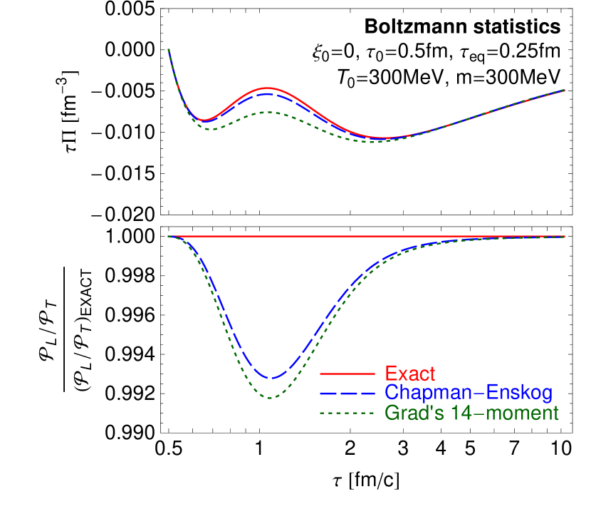
Figure 2: (Color online) Time evolution of the the bulk viscous pressure times $\tau$ (top) and the pressure anisotropy ${\cal P}_{L}/{\cal P}_{T}$ scaled by that obtained using exact solution of the RTA Boltzmann equation (bottom) for Boltzmann statistics. The three curves in both panels correspond to three different calculations: the exact solution of the RTA Boltzmann equation Florkowski:2014sda (red solid line), second-order viscous hydrodynamics obtained using the Chapman-Enskog method (blue dashed line) and using the Grad’s 14-moment approximation (green dotted line). For both panels we use $T_{0}=300$ MeV at $\tau_{0}=0.5$ fm/c, $m=300$ MeV, and $\tau_{\rm eq}=\tau_{\pi}=\tau_{\Pi}=0.25$ fm/c. The initial spheroidal anisotropy in the distribution function, $\xi_{0}=0$, corresponds to isotropic initial pressures with $\Pi_{0}=\pi_{0}=0$.

In Fig. 1, we show $m/T$ dependence of the ratio $\zeta/\eta$ scaled by $(1/3-c_{s}^{2})^{2}$ for various cases. We observe that in accordance with the predictions from small-$z$ expansion, Eq. (57), the curve for Boltzmann statistics (red solid line) and Fermi-Dirac statistics (green dotted line) saturates at $75$ and $48$ (thin horizontal black dashed lines), respectively, at small values of $z$. We also see that at very small-$z$, Bose-Einstein statistics (blue dashed line) results in very large values of the scaled viscosity ratio $(\zeta/\eta)/(1/3-c_{s}^{2})^{2}$ indicating divergence. We see that this ratio for the QGP is dominated by the Bose-Einstein statistics for two-flavor (brown dashed-dotted line) as well as three-flavor QGP (purple dashed-dotted-dotted line). This however does not imply that the bulk viscosity of QGP is very large because a realistic calculation with lattice QCD equation of state suggest that $z>0.6$ even for temperatures as high as central RHIC and LHC energies Romatschke:2011qp ; Andersen:2011sf ; Strickland:2014zka . Moreover, for large-$z$ we see that all three statistics lead to similar results for the scaled viscosity ratio which suggests that there is a relatively small effect coming from composition of the fluid.

VI Boost-invariant 0+1d case

In this section, we consider evolution in the case of transversely homogeneous and purely-longitudinal boost-invariant expansion Bjorken:1982qr . For such an expansion all scalar functions of space and time depend only on the longitudinal proper time $\tau=\sqrt{t^{2}-z^{2}}$. Working in the Milne coordinate system, $(\tau,x,y,\eta)$, the hydrodynamic four-velocity is given by $u^{\mu}=(1,0,0,0)$. The energy-momentum conservation equation together with Eqs. (23) and (24) reduce to

$$\dot{\epsilon} =-\frac{1}{\tau}\left(\epsilon+P+\Pi-\pi\right)\,,$$ (60)

$$\dot{\Pi}+\frac{\Pi}{\tau_{\Pi}} =-\frac{\beta_{\Pi}}{\tau}-\delta_{\Pi\Pi}\frac{\Pi}{\tau}+\lambda_{\Pi\pi}\frac{\pi}{\tau}\,,$$ (61)

$$\dot{\pi}+\frac{\pi}{\tau_{\pi}} =\frac{4}{3}\frac{\beta_{\pi}}{\tau}-\left(\frac{1}{3}\tau_{\pi\pi}+\delta_{\pi\pi}\right)\frac{\pi}{\tau}+\frac{2}{3}\lambda_{\pi\Pi}\frac{\Pi}{\tau}\,,$$ (62)

where $\pi\equiv-\tau^{2}\pi^{\eta\eta}$. Note that in this case the term involving the vorticity tensor in Eq. (24) vanishes and hence has no effect on the dynamics of the fluid. Also note that the first terms on the right-hand side of Eqs. (61) and (62) corresponds to the first-order terms $\beta_{\Pi}\theta$ and $2\beta_{\pi}\sigma^{\mu\nu}$, respectively, whereas the rest are of second-order.

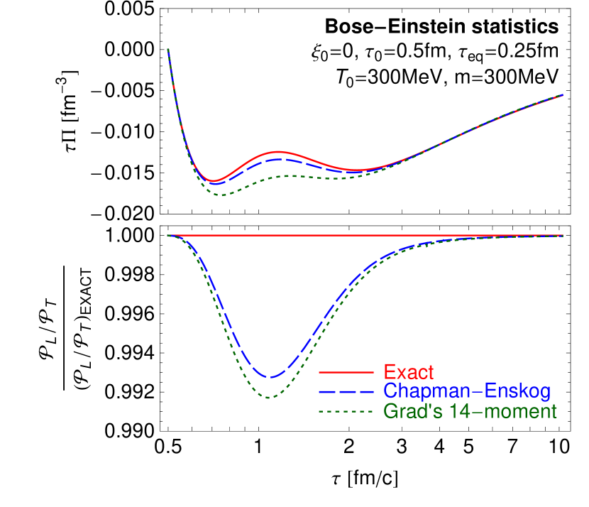
Figure 3: (Color online) Same as Fig. 2 except here we consider Bose-Einstein statistics.

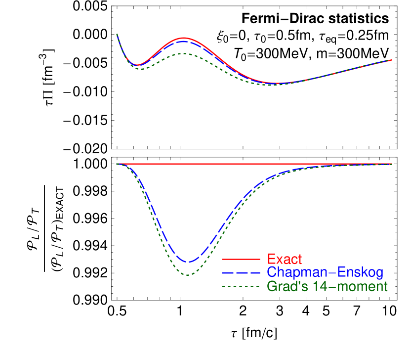
Figure 4: (Color online) Same as Fig. 2 except here we consider Fermi-Dirac statistics.

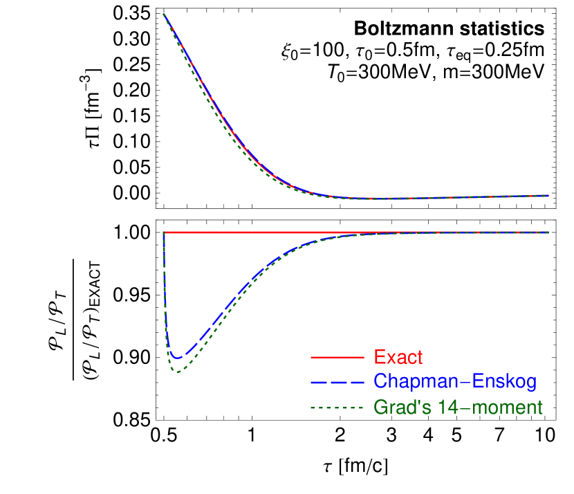
Figure 5: (Color online) Same as Fig. 2 except here we take $\xi_{0}=100$ corresponding to $\pi_{0}=2.86$ GeV/fm³ and $\Pi_{0}=0.138$ GeV/fm³.

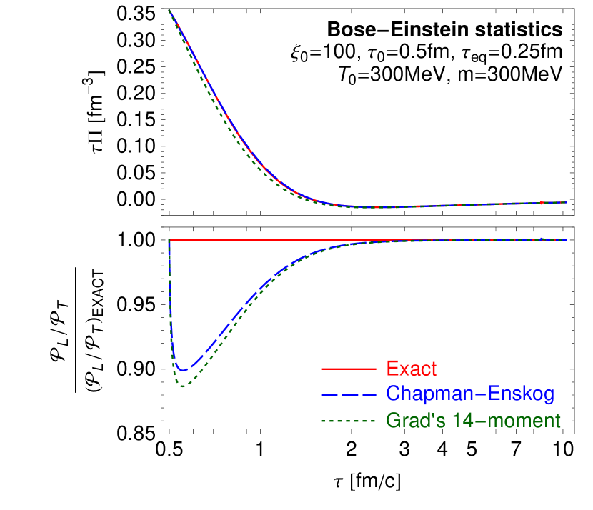
Figure 6: (Color online) Same as Fig. 5 except here we consider Bose-Einstein statistics.

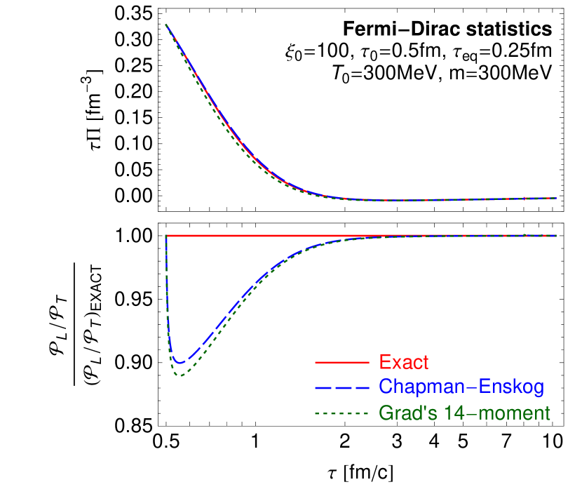
Figure 7: (Color online) Same as Fig. 5 except here we consider Fermi-Dirac statistics.

We simultaneously solve Eqs. (60)-(62) assuming an initial temperature of $T_{0}=300$ MeV at the initial proper time $\tau_{0}=0.5$ fm/c, with relaxation times $\tau_{\rm eq}=\tau_{\Pi}=\tau_{\pi}=0.25$ fm/c corresponding to initial $\eta/s=1/4\pi$. We solve these equations for two different initial pressure configurations: $\xi_{0}=0$ corresponding to an isotropic pressure configuration $\pi_{0}=\Pi_{0}=0$ and $\xi_{0}=100$ corresponding to a highly oblate anisotropic pressure configuration. The anisotropy parameter $\xi$ is related to the average longitudinal and transverse momentum in the local rest frame as: $\xi=\frac{1}{2}\langle p_{T}^{2}\rangle/\langle p_{L}^{2}\rangle-1$, where $\langle\cdots\rangle\equiv\int d^{3}pf_{0}(\sqrt{p_{T}^{2}+(1+\xi)p_{L}^{2}},\Lambda)$ and $\Lambda$ is a temperature-like scale which can be identified with the temperature of the system in the isotropic equilibrium limit. For particle mass, we consider $m=300$ MeV which roughly corresponds to the constituent quark mass. We solve Eqs. (60)-(62) with transport coefficients obtained using the Grad’s 14-moment method, Eqs. (25)-(29), as well as the Chapman-Enskog method, Eqs. (32)-(36).

In Figs. 2 – 7 we show the time evolution of the bulk viscous pressure times proper-time (top) and the pressure anisotropy ${\cal P}_{L}/{\cal P}_{T}\equiv(P+\Pi-\pi)/(P+\Pi+\pi/2)$ scaled by that obtained using exact solution of the RTA Boltzmann equation (bottom) for three different calculations: the exact solution of the RTA Boltzmann equation Florkowski:2014sda (red solid line), second-order viscous hydrodynamics obtained using the Chapman-Enskog method, Eqs. (32)-(36), (blue dashed line) and using the Grad’s 14-moment approximation, Eqs. (25)-(29), (green dotted line). Figures 2 and 5 are for Boltzmann statistics, Figs. 3 and 6 are for Bose-Einstein statistics, and Figs. 4 and 7 are for Fermi-Dirac statistics. Figs. 2 – 4 correspond to an isotropic initial condition ($\xi_{0}=0$), while Figs. 5 – 7 correspond to a highly oblate anisotropic initial condition ($\xi_{0}=100$).

From Figs. 2 – 7, we observe that, compared to Grad’s 14-moment approximation, the transport coefficients obtained using the Chapman-Enskog method does a marginally better job in reproducing the ${\cal P}_{L}/{\cal P}_{T}$ obtained using the exact solution of the RTA Boltzmann equation. On the other hand, the result for $\tau\Pi$ obtained using the Chapman-Enskog method shows better agreement with the exact solution of the RTA Boltzmann equation than the Grad’s 14-moment method.

VII Conclusions and outlook

In this paper we expressed the transport coefficients appearing in the second-order viscous hydrodynamical evolution of a massive gas using Bose-Einstein, Boltzmann and Fermi-Dirac statistics for the equilibrium distribution function and Grad’s 14-moment approximation as well as the method of Chapman-Enskog expansion for the non-equilibrium part. The second-order viscous evolution equations are obtained by coarse graining the relativistic Boltzmann equation in the relaxation-time approximation. We also obtained the ratio of the coefficient of bulk viscosity to that of shear viscosity, in terms of the speed of sound, for classical and quantum statistics as well as for the QGP. We then considered the specific case of a transversally homogeneous and longitudinally boost-invariant system for which it is possible to exactly solve the RTA Boltzmann equation Florkowski:2014sda . Using this solution as a benchmark, we compared the pressure anisotropy and bulk viscous pressure evolution obtained by employing both the Chapman-Enskog method as well as the Grad’s 14-moment method. We demonstrated that the Chapman-Enskog method is in better agreement with the exact solution of the RTA Boltzmann equation compared to the Grad’s 14-moment method. We found that, while both methods give similar results for the pressure anisotropy, the Chapman-Enskog method better reproduces the exact solution for the bulk viscous pressure evolution.

At this juncture, we would like to clarify that we have used the exact solution of the Boltzmann equation, in the relaxation-time approximation, as a benchmark in order to compare different hydrodynamic formulations. The relaxation-time approximation is based on the assumption that the collisions tend to restore the phase-space distribution function to its equilibrium value exponentially. Although the microscopic interactions of the constituent particles are not captured in this approximation, it is reasonably accurate to describe a system which is close to local thermodynamic equilibrium Dusling:2009df . Looking forward, it will be interesting to determine the impact of the quantum transport coefficients, obtained herein, in higher dimensional simulations. Moreover, it would also be instructive to see if the second-order results derived herein could be extended to obtain third order transport coefficients for quantum statistics Jaiswal:2013vta . We leave these questions for a future work.

- (1) U. Heinz and R. Snellings, Ann. Rev. Nucl. Part. Sci. 63, 123 (2013).
- (2) L.D. Landau and E.M. Lifshitz, Fluid Mechanics (Butterworth-Heinemann, Oxford, 1987).
- (3) C. Eckart, Phys. Rev. 58, 267 (1940).
- (4) W. Israel and J. M. Stewart, Annals Phys. (N.Y.) 118, 341 (1979).
- (5) P. Romatschke, Int. J. Mod. Phys. E 19, 1 (2010).
- (6) A. Muronga, Phys. Rev. C 69, 034903 (2004).
- (7) A. El, Z. Xu and C. Greiner, Phys. Rev. C 81, 041901(R) (2010).
- (8) G. S. Denicol, H. Niemi, E. Molnar and D. H. Rischke, Phys. Rev. D 85, 114047 (2012).
- (9) G. S. Denicol, T. Koide and D. H. Rischke, Phys. Rev. Lett. 105, 162501 (2010).
- (10) A. Jaiswal, R. S. Bhalerao and S. Pal, Phys. Lett. B 720, 347 (2013); J. Phys. Conf. Ser. 422, 012003 (2013); arXiv:1303.1892 [nucl-th].
- (11) A. Jaiswal, R. S. Bhalerao and S. Pal, Phys. Rev. C 87, 021901(R) (2013).
- (12) R. S. Bhalerao, A. Jaiswal, S. Pal and V. Sreekanth, Phys. Rev. C 88, 044911 (2013).
- (13) G. S. Denicol, S. Jeon and C. Gale, Phys. Rev. C 90, 024912 (2014).
- (14) G. S. Denicol, W. Florkowski, R. Ryblewski and M. Strickland, Phys. Rev. C 90, 044905 (2014).
- (15) R. S. Bhalerao, A. Jaiswal, S. Pal and V. Sreekanth, Phys. Rev. C 89, 054903 (2014).
- (16) A. Jaiswal, Phys. Rev. C 87, 051901(R) (2013); arXiv:1408.0867 [nucl-th].
- (17) A. Jaiswal, Phys. Rev. C 88, 021903(R) (2013); Nucl. Phys. A 931, 1205 (2014).
- (18) A. Jaiswal, R. Ryblewski and M. Strickland, Phys. Rev. C 90, 044908 (2014).
- (19) C. Chattopadhyay, A. Jaiswal, S. Pal and R. Ryblewski, Phys. Rev. C 91, 024917 (2015).
- (20) M. Prakash, M. Prakash, R. Venugopalan and G. Welke, Phys. Rept. 227, 321 (1993).
- (21) D. Davesne, Phys. Rev. C 53, 3069 (1996).
- (22) A. Wiranata and M. Prakash, Phys. Rev. C 85, 054908 (2012).
- (23) A. Wiranata, M. Prakash and P. Chakraborty, Central Eur. J. Phys. 10, 1349 (2012).
- (24) A. Wiranata, M. Prakash, P. Huovinen, V. Koch and X. N. Wang, J. Phys. Conf. Ser. 535, 012017 (2014).
- (25) P. Romatschke and M. Strickland, Phys. Rev. D 68, 036004 (2003).
- (26) W. Florkowski and R. Ryblewski, Phys. Rev. C 83, 034907 (2011).
- (27) M. Martinez and M. Strickland, Nucl. Phys. A 848, 183 (2010).
- (28) W. Florkowski, R. Ryblewski and M. Strickland, Nucl. Phys. A 916, 249 (2013); Phys. Rev. C 88, (2013) 024903.
- (29) D. Bazow, U. W. Heinz and M. Strickland, Phys. Rev. C 90, 054910 (2014).
- (30) M. Nopoush, R. Ryblewski and M. Strickland, Phys. Rev. C 90, 014908 (2014).
- (31) W. Florkowski, R. Ryblewski, M. Strickland and L. Tinti, Phys. Rev. C 89, 054909 (2014).
- (32) W. Florkowski, E. Maksymiuk, R. Ryblewski and M. Strickland, Phys. Rev. C 89, 054908 (2014).
- (33) W. Florkowski and E. Maksymiuk, J. Phys. G 42, 045106 (2015).
- (34) H. Grad, Comm. Pure Appl. Math. 2, 331 (1949).
- (35) S. Chapman and T. G. Cowling, The Mathematical Theory of Non-uniform Gases (Cambridge University Press, Cambridge, 1970), 3rd ed.
- (36) P. Romatschke and U. Romatschke, Phys. Rev. Lett. 99, 172301 (2007).
- (37) H. Song, S. A. Bass, U. Heinz, T. Hirano and C. Shen, Phys. Rev. Lett. 106, 192301 (2011) [Erratum-ibid. 109, 139904 (2012)].
- (38) B. Schenke, S. Jeon and C. Gale, Phys. Rev. C 85, 024901 (2012).
- (39) G. Policastro, D. T. Son and A. O. Starinets, Phys. Rev. Lett. 87, 081601 (2001).
- (40) P. Kovtun, D. T. Son and A. O. Starinets, Phys. Rev. Lett. 94, 111601 (2005).
- (41) S. Gavin, Nucl. Phys. A 435, 826 (1985).
- (42) G. D. Moore and O. Saremi, JHEP 0809, 015 (2008).
- (43) A. Wiranata and M. Prakash, Nucl. Phys. A 830, 219C (2009).
- (44) P. Chakraborty and J. I. Kapusta, Phys. Rev. C 83, 014906 (2011).
- (45) J. Noronha-Hostler, J. Noronha and F. Grassi, Phys. Rev. C 90, 034907 (2014).
- (46) J. B. Rose, J. F. Paquet, G. S. Denicol, M. Luzum, B. Schenke, S. Jeon and C. Gale, Nucl. Phys. A 931, 926 (2014).
- (47) S. Ryu, J.-F. Paquet, C. Shen, G. S. Denicol, B. Schenke, S. Jeon and C. Gale, arXiv:1502.01675 [nucl-th].
- (48) S.R. de Groot, W.A. van Leeuwen, and Ch.G. van Weert, Relativistic Kinetic Theory: Principles and Applications (North-Holland, Amsterdam, 1980).
- (49) P. Romatschke, Phys. Rev. D 85, 065012 (2012).
- (50) J. L. Anderson and H. R. Witting Physica 74, 466 (1974).
- (51) S. Weinberg, Gravitation and Cosmology (Wiley, 1972); Astrophys. J. 168, 175 (1971).
- (52) J. O. Andersen, L. E. Leganger, M. Strickland and N. Su, JHEP 1108, 053 (2011).
- (53) M. Strickland, J. O. Andersen, A. Bandyopadhyay, N. Haque, M. G. Mustafa and N. Su, Nucl. Phys. A 931, 841 (2014).
- (54) J. D. Bjorken, Phys. Rev. D 27, 140 (1983).
- (55) K. Dusling, G. D. Moore and D. Teaney, Phys. Rev. C 81, 034907 (2010).