Abstract

For the problem of high-dimensional sparse linear regression, it is known that an $\ell_{0}$-based estimator can achieve a $1/n$ “fast” rate on the prediction error without any conditions on the design matrix, whereas in the absence of restrictive conditions on the design matrix, popular polynomial-time methods only guarantee the $1/\sqrt{n}$ “slow” rate. In this paper, we show that the slow rate is intrinsic to a broad class of M-estimators. In particular, for estimators based on minimizing a least-squares cost function together with a (possibly non-convex) coordinate-wise separable regularizer, there is always a “bad” local optimum such that the associated prediction error is lower bounded by a constant multiple of $1/\sqrt{n}$. For convex regularizers, this lower bound applies to all global optima. The theory is applicable to many popular estimators, including convex $\ell_{1}$-based methods as well as M-estimators based on nonconvex regularizers, including the SCAD penalty or the MCP regularizer. In addition, we show that the bad local optima are very common, in that a broad class of local minimization algorithms with random initialization will typically converge to a bad solution.

1 Introduction

The classical notion of minimax risk, which plays a central role in decision theory, allows for the statistician to implement any possible estimator, regardless of its computational cost. For many problems, there are a variety of estimators, which can be ordered in terms of their computational complexity. Given that it is usually feasible only to implement polynomial-time methods, it has become increasingly important to study computationally-constrained analogues of the minimax estimator, in which the choice of estimator is restricted to a subset of computationally efficient estimators [32]. A fundamental question is when such computationally-constrained forms of minimax risk estimation either coincide or differ in a fundamental way from their classical counterpart.

The goal of this paper is to explore such gaps between classical and computationally practical minimax risks, in the context of prediction error for high-dimensional sparse regression. Our main contribution is to establish a fundamental gap between the classical minimax prediction risk and the best possible risk achievable by a broad class of $M$-estimators based on coordinate-separable regularizers, one which includes various nonconvex regularizers that are used in practice.

In more detail, the classical linear regression model is based on a response vector $y\in\mathbb{R}^{n}$ and a design matrix $X\in\mathbb{R}^{n\times d}$ that are linked via the relationship

$$y =X\theta^{*}+w,$$ (1)

where the vector $w\in\mathbb{R}^{n}$ is a random noise vector. Our goal is to estimate the unknown regression vector $\theta^{*}\in\mathbb{R}^{d}$. Throughout this paper, we focus on the standard Gaussian model, in which the entries of the noise vector $w$ are i.i.d. $N(0,\sigma^{2})$ variates, and the case of deterministic design, in which the matrix $X$ is viewed as non-random. In the sparse variant of this model, the regression vector is assumed to have a small number of non-zero coefficients. In particular, for some positive integer $k<d$, the vector $\theta^{*}$ is said to be $k$-sparse if it has at most $k$ non-zero coefficients. Thus, the model is parameterized by the triple $(n,d,k)$ of sample size $n$, ambient dimension $d$, and sparsity $k$. We use $\mathbb{B}_{0}(k)$ to the denote the $\ell_{0}$-“ball” of all $d$-dimensional vectors with at most $k$ non-zero entries.

An estimator $\widehat{\theta}$ is a measurable function of the pair $(y,X)$, taking values in $\mathbb{R}^{d}$, and its quality can be assessed in different ways. In this paper, we focus on its fixed design prediction error, given by $\mathbb{E}\big{[}\frac{1}{n}\|X(\widehat{\theta}-\theta^{*})\|_{2}^{2}\big{]}$, a quantity that measures how well $\widehat{\theta}$ can be used to predict the vector $X\theta^{*}$ of noiseless responses. The worst-case prediction error of an estimator $\widehat{\theta}$ over the set $\mathbb{B}_{0}(k)$ is given by

$$\mathcal{M}_{n,k,d}(\widehat{\theta};X) :\,=\sup_{\theta^{*}\in\mathbb{B}_{0}(k)}\frac{1}{n}\mathbb{E}[\|{X(\widehat{\theta}-\theta^{*})}\|_{2}^{2}]$$ (2)

Given that $\theta^{*}$ is $k$-sparse, the most direct approach would be to seek a $k$-sparse minimizer to the least-squares cost $\|y-X\theta\|_{2}^{2}$, thereby obtaining the $\ell_{0}$-based estimator

$$\widehat{\theta}_{\ell_{0}} \in\arg\min_{\theta\in\mathbb{B}_{0}(k)}\|y-X\theta\|_{2}^{2}.$$ (3)

The $\ell_{0}$-based estimator $\widehat{\theta}_{\ell_{0}}$ is known [7, 28] to satisfy a bound of the form

$$\mathcal{M}_{n,k,d}(\widehat{\theta}_{\ell_{0}};X)\precsim\frac{\sigma^{2}\,k\log d}{n},$$ (4)

where $\precsim$ denotes an inequality up to constant factors (independent of the triple $(n,d,k)$ as well as the standard deviation $\sigma$). However, it is not tractable to compute this estimator in a brute force manner, since there are ${d\choose k}$ subsets of size $k$ to consider.

The computational intractability of the $\ell_{0}$-based estimator has motivated the use of various heuristic algorithms and approximations, including the basis pursuit method [10], the Dantzig selector [8], as well as the extended family of Lasso estimators [30, 10, 36, 2]. Essentially, these methods are based on replacing the $\ell_{0}$-constraint with its $\ell_{1}$-equivalent, in either a constrained or penalized form. There is now a very large body of work on the performance of such methods, covering different criteria including support recovery, $\ell_{2}$-norm error and prediction error (e.g., see the book [6] and references therein).

For the case of fixed design prediction error that is the primary focus here, such $\ell_{1}$-based estimators are known to achieve the bound (4) only if the design matrix $X$ satisfies certain conditions, such as the restricted eigenvalue (RE) condition or compatibility condition [4, 31] or the stronger restricted isometry property [8]; see the paper [31] for an overview of these various conditions, and their inter-relationships. Without such conditions, the best known guarantees for $\ell_{1}$-based estimators are of the form

$$\mathcal{M}_{n,k,d}(\widehat{\theta}_{\ell_{1}};X)\precsim\sigma\,R\,\sqrt{\frac{\log d}{n}},$$ (5)

a bound that is valid without any RE conditions on the design matrix $X$ whenever the $k$-sparse regression vector $\theta^{*}$ has $\ell_{1}$-norm bounded by $R$ (e.g., see the papers [7, 26, 28].)

The substantial gap between the “fast” rate (4) and the “slow” rate (5) leaves open a fundamental question: is there a computationally efficient estimator attaining the bound (4) for general design matrices? In the following subsections, we provide an overview of the currently known results on this gap, and we then provide a high-level statement of the main result of this paper.

1.1 Lower bounds for Lasso

Given the gap between the fast rate (4) and the Lasso’s slower rate (5), one possibility might be that existing analyses of prediction error are overly conservative, and $\ell_{1}$-based methods can actually achieve the bound (4), without additional constraints on $X$. Some past work has given negative answers to this quesiton. Foygel and Srebro [15] constructed a 2-sparse regression vector and a random design matrix for which the Lasso prediction error with any choice of regularization parameter $\lambda_{n}$ is lower bounded by $1/\sqrt{n}$. In particular, their proposed regression vector is $\theta^{*}=(0,\dots,0,\frac{1}{2},\frac{1}{2})$. In their design matrix, the columns are randomly generated with distinct covariances, and moreover, such that the rightmost column is strongly correlated with the other two columns on its left. With this particular regression vector and design matrix, they show that Lasso’s prediction error is lower bounded by $1/\sqrt{n}$ for any choice of Lasso regularization parameter $\lambda$. This construction is explicit for Lasso, and thus does not apply to more general M-estimators. Moreover, for this particular counterexample, there is a one-to-one correspondence between the regression vector and the design matrix, so that one can identify the non-zero coordinates of $\theta^{*}$ by examining the design matrix. Consequently, for this construction, a simple reweighted form of the Lasso can be used to achieve the fast rate. In particular, the reweighted Lasso estimator

$$\widehat{\theta}_{\rm wl}\in\arg\min_{\theta\in{\mathbb{R}}^{d}}\left\{\|y-X\theta\|_{2}^{2}+\lambda\sum_{j=1}^{d}\alpha_{j}|\theta_{j}|\right\},$$ (6)

with $\lambda$ chosen in the usual manner ($\lambda\asymp\sigma\sqrt{\frac{\log d}{n}}$), weights $\alpha_{d-1}=\alpha_{d}=1$, and the remaining weights $\{\alpha_{1},\ldots,\alpha_{d-2}\}$ chosen to be sufficiently large, has this property. Dalalyan et al. [12] construct a stronger counter-example, for which the prediction error of Lasso is again lower bounded by $1/\sqrt{n}$. For this counterexample, there is no obvious correspondence between the regression vector and the design matrix. Nevertheless, as we show in Appendix A, the reweighted Lasso estimator (6) with a proper choice of the regularization coefficients still achieves the fast rate on this example. Another related piece of work is by Candès and Plan [9]. They construct a design matrix for which the Lasso estimator, when applied with the usual choice of regularization parameter $\lambda\asymp\sigma(\frac{\log d}{n})^{1/2}$, has sub-optimal prediction error. Their matrix construction is spiritually similar to ours, but the theoretical analysis is limited to the Lasso for a particular choice of regularization parameter. It does not rule out the possibility that other choices of regularization parameters, or other polynomial-time estimators can achieve the fast rate. In contrast, our hardness result applies to general $M$-estimators based on coordinatewise separable regularizers, and it allows for arbitrary regularization parameters.

1.2 Complexity-theoretic lower bound for polynomial-time sparse estimators

In our own recent work [35], we have provided a complexity-theoretic lower bound that applies to a very broad class of polynomial-time estimators. The analysis is performed under a standard complexity-theoretic condition—namely, that the class ${\bf NP}$ is not a subset of the class ${\bf P/poly}$—and shows that there is no polynomial-time algorithm that returns a $k$-sparse vector that achieves the fast rate. The lower bound is established as a function of the restricted eigenvalue of the design matrix. Given sufficiently large $(n,k,d)$ and any $\gamma>0$, a design matrix $X$ with restricted eigenvalue $\gamma$ can be constructed, such that every polynomial-time $k$-sparse estimator $\widehat{\theta}_{\rm poly}$ has its minimax prediction risk lower bounded as

$$\mathcal{M}_{n,k,d}(\widehat{\theta}_{\rm poly};X)\succsim\frac{\sigma^{2}\,k^{1-\delta}\log d}{\gamma n},$$ (7)

where $\delta>0$ is an arbitrarily small positive scalar. Note that the fraction $k^{-\delta}/\gamma$, which characterizes the gap between the fast rate and the rate (7), could be arbitrarily large. The lower bound has the following consequence: any estimator that achieves the fast rate must either not be polynomial-time, or must return a regression vector that is not $k$-sparse.

The condition that the estimator is $k$-sparse is essential in the proof of lower bound (7). In particular, the proof relies on a reduction between estimators with low prediction error in the sparse linear regression model, and methods that can solve the 3-set covering problem [24], a classical problem that is known to be NP-hard. The 3-set covering problem takes as input a list of 3-sets, which are subsets of a set $\mathcal{S}$ whose cardinality is $3k$. The goal is to choose $k$ of these subsets in order to cover the set $\mathcal{S}$. The lower bound (7) is established by showing that if there is a $k$-sparse estimator achieving better prediction error, then it provides a solution to the 3-set covering problem, as every non-zero coordinate of the estimate corresponds to a chosen subset. This hardness result does not eliminate the possibility of finding a polynomial-time estimator that returns dense vectors satisfying the fast rate. In particular, it is possible that a dense estimator cannot be used to recover a a good solution to the 3-set covering problem, implying that it is not possible to use the hardness of $3$-set covering to assert the hardness of achieving low prediction error in sparse regression.

At the same time, there is some evidence that better prediction error can be achieved by dense estimators. For instance, suppose that we consider a sequence of high-dimensional sparse linear regression problems, such that the restricted eigenvalue $\gamma=\gamma_{n}$ of the design matrix $X\in\mathbb{R}^{n\times d}$ decays to zero at the rate $\gamma_{n}=1/n^{2}$. For such a sequence of problems, as $n$ diverges to infinity, the lower bound (7), which applies to $k$-sparse estimators, goes to infinity, whereas the Lasso upper bound (5) converges to zero. Although this behavior is somewhat mysterious, it is not a contradiction. Indeed, what makes Lasso’s performance better than the lower bound (7) is that it allows for non-sparse estimates. In this example, truncating the Lasso’s estimate to be $k$-sparse will substantially hurt the prediction error. In this way, we see that proving lower bounds for non-sparse estimators—the problem to be addressed in this paper—is a substantially more challenging task than proving lower bound for estimators that must return sparse outputs.

1.3 Main results of this paper

With this context in place, let us now turn to a high-level statement of the main results of this paper. More precisely, our contribution is to provide additional evidence against the polynomial achievability of the fast rate (4), in particular by showing that the slow rate (5) is a lower bound for a broad class of M-estimators, namely those based on minimizing a least-squares cost function together with a coordinate-wise decomposable regularizer. In particular, we consider estimators that are based on an objective function of the form $L(\theta;\lambda)=\frac{1}{n}\|y-X\theta\|_{2}^{2}+\lambda\,\rho(\theta)$, for a weighted regularizer $\rho:\mathbb{R}^{d}\rightarrow\mathbb{R}$ that is coordinate-separable. See Section 2.1 for a precise definition of this class of estimators. Our first main result (Theorem 1) establishes that there is always a matrix $X\in{\mathbb{R}}^{n\times d}$ such that for any coordinate-wise separable function $\rho$ and for any choice of weight $\lambda\geq 0$, the objective $L$ always has at least one local optimum $\widehat{\theta}_{\lambda}$ such that

$$\sup_{\theta^{*}\in\mathbb{B}_{0}(k)}\mathbb{E}\Big{[}\frac{1}{n}\|{X(\widehat{\theta}_{\lambda}-\theta^{*}\big{)}}\|_{2}^{2}\Big{]}\succsim\frac{\sigma}{\sqrt{n}}.$$ (8)

Moreover, if the regularizer $\rho$ is convex, then this lower bound applies to all global optima of the convex criterion $L$. This lower bound is applicable to many popular estimators, including the ridge regression estimator [19], the basis pursuit method [10], the Lasso estimator [30], the weighted Lasso estimator [36], the square-root Lasso estimator [2], and least squares based on nonconvex regularizers such as the SCAD penalty [14] or the MCP penalty [34].

In the nonconvex setting, it is impossible (in general) to guarantee anything beyond local optimality for any solution found by a polynomial-time algorithm [17]. Nevertheless, to play the devil’s advocate, one might argue that the assumption that an adversary is allowed to pick a bad local optimum could be overly pessimistic for statistical problems. In order to address this concern, we prove a second result (Theorem 2) that demonstrates that bad local solutions are difficult to avoid. Focusing on a class of local descent methods, we show that given a random isotropic initialization centered at the origin, the resulting stationary points have poor mean-squared error—that is, they can only achieve the slow rate. In this way, this paper shows that the gap between the fast and slow rates in high-dimensional sparse regression cannot be closed via standard application of a very broad class of methods. In conjunction with our earlier complexity-theoretic paper [35], it adds further weight to the conjecture that there is a fundamental gap between the performance of polynomial-time and exponential-time methods for sparse prediction.

The remainder of this paper is organized as follows. We begin in Section 2 with further background, including a precise definition of the family of $M$-estimators considered in this paper, some illustrative examples, and discussion of the prediction error bound achieved by the Lasso. Section 3 is devoted to the statements of our main results, along with discussion of their consequences. In Section 4, we provide the proofs of our main results, with some technical lemmas deferred to the appendices. We conclude with a discussion in Section 5.

2 Background and problem set-up

As previously described, an instance of the sparse linear regression problem is based on observing a pair $(X,y)\in{\mathbb{R}}^{n\times d}\times{\mathbb{R}}^{n}$ of instances that are linked via the linear model (1), where the unknown regressor $\theta^{*}$ is assumed to be $k$-sparse, and so belongs to the $\ell_{0}$-ball $\mathbb{B}_{0}(k)$. Our goal is to find a good predictor, meaning a vector $\widehat{\theta}$ such that the mean-squared prediction error $\frac{1}{n}\|{X(\widehat{\theta}-\theta^{*})}\|_{2}^{2}$ is small.

2.1 Least squares with coordinate-separable regularizers

The analysis of this paper applies to estimators that are based on minimizing a cost function of the form

$$L(\theta;\lambda) =\frac{1}{n}\|y-X\theta\|_{2}^{2}+\lambda\,\rho(\theta),$$ (9)

where $\rho:\mathbb{R}^{d}\rightarrow\mathbb{R}$ is a regularizer, and $\lambda\geq 0$ is a regularization weight. We consider the following family $\mathcal{F}$ of coordinate-separable regularizers:

1. The function $\rho:\mathbb{R}^{d}\rightarrow\mathbb{R}$ is coordinate-wise decomposable, meaning that $\rho(\theta)=\sum_{j=1}^{d}\rho_{j}(\theta_{j})$ for some univariate functions $\rho_{j}:\mathbb{R}\rightarrow\mathbb{R}$.

2. Each univariate function satisfies $\rho_{j}(0)=0$ and is symmetric around zero (i.e., $\rho_{j}(t)=\rho_{j}(-t)$ for all $t\in{\mathbb{R}}$).

3. On the nonnegative real line $[0,+\infty)$, each function $\rho_{j}$ is nondecreasing.

Let us consider some examples to illustrate this definition.

Bridge regression:

The family of bridge regression estimates [16] take the form

$$\widehat{\theta}_{\tiny{\mbox{bidge}}}\in\arg\min_{\theta\in\mathbb{R}^{d}}\Big{\{}\frac{1}{n}\|y-X\theta\|_{2}^{2}+\lambda\sum_{i=1}^{d}|\theta|^{\gamma}\Big{\}}.$$

Note that this is a special case of the objective function (9) with $\rho_{j}(\cdot)=|\cdot|^{\gamma}$ for each coordinate. When $\gamma\in\{1,2\}$, it corresponds to the Lasso estimator and the ridge regression estimator respectively. The analysis of this paper provides lower bounds for both estimators, uniformly over the choice of $\lambda$.

Weighted Lasso:

The weighted Lasso estimator [36] uses a weighted $\ell_{1}$-norm to regularize the empirical risk, and leads to the estimator

$$\widehat{\theta}_{\tiny{\mbox{wl}}}\in\arg\min_{\theta\in\mathbb{R}^{d}}\Big{\{}\frac{1}{n}\|y-X\theta\|_{2}^{2}+\lambda\sum_{i=1}^{d}\alpha_{i}|\theta_{i}|\Big{\}}.$$

Here $\alpha_{1},\dots,\alpha_{d}$ are weights that can be adaptively chosen with respect to the design matrix $X$. The weighted Lasso can perform better than the ordinary Lasso, corresponding to the special case in which all $\alpha_{j}$ are all equal. For instance, on the counter-example proposed by Foygel and Srebro [15], for which the ordinary Lasso estimator achieves only the slow $1/\sqrt{n}$ rate, the weighted Lasso estimator achieves the $1/n$ convergence rate. Nonetheless, the analysis of this paper shows that there are design matrices for which the weighted Lasso, even when the weights are chosen adaptively with respect to the design, has prediction error at least a constant multiple of $1/\sqrt{n}$.

Square-root Lasso:

The square-root Lasso estimator [2] is defined by minimizing the criterion

$$\widehat{\theta}_{\tiny{\mbox{sqrt}}}\in\arg\min_{\theta\in\mathbb{R}^{d}}\Big{\{}\frac{1}{\sqrt{n}}\|y-X\theta\|_{2}+\lambda\left\|{\theta}\right\|_{1}\Big{\}}.$$

This criterion is slightly different from our general objective function (9), since it involves the square root of the least-squares error. Relative to the Lasso, its primary advantage is that the optimal setting of the regularization parameter does not require the knowledge of the standard deviation of the noise. For the purposes of the current analysis, it suffices to note that by Lagrangian duality, every square-root Lasso estimate $\widehat{\theta}_{\tiny{\mbox{sqrt}}}$ is a minimizer of the least-squares criterion $\|y-X\theta\|_{2}$, subject to $\|\theta\|_{1}\leq R$, for some radius $R\geq 0$ depending on $\lambda$. Consequently, as the weight $\lambda$ is varied over the interval $[0,\infty)$, the square root Lasso yields the same solution path as the Lasso. Since our lower bounds apply to the Lasso for any choice of $\lambda\geq 0$, they also apply to all square-root Lasso solutions.

Figure 1: Plots with regularization weight $\lambda=1$, and parameters $a=3.7$ for SCAD, and $b=2.7$ for MCP.

SCAD penalty or MCP regularizer:

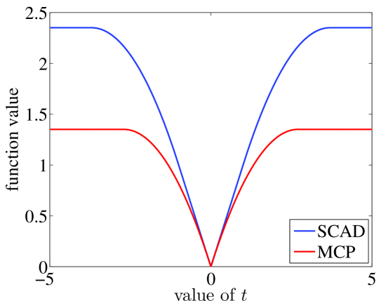
Due to the intrinsic bias induced by $\ell_{1}$-regularization, various forms of nonconvex regularization are widely used. Two of the most popular are the SCAD penalty, due to Fan and Li [14], and the MCP penalty, due to Zhang et al. [34]. The family of SCAD penalties takes the form

$$\phi_{\lambda}(t):=\frac{1}{\lambda}\begin{cases}\lambda|t|&\mbox{for $|t|\leq\lambda$},\\ -(t^{2}-2a\lambda|t|+\lambda^{2})/(2a-2)&\mbox{for $\lambda<|t|\leq a\lambda$},\\ (a+1)\lambda^{2}/2&\mbox{for $|t|\geq a\lambda$},\end{cases}$$

where $a>2$ is a fixed parameter. When used with the least-squares objective, it is a special case of our general set-up with $\rho_{j}(\theta_{j})=\phi_{\lambda}(\theta_{j})$ for each coordinate $j=1,\ldots,d$. Similarly, the MCP penalty takes the form

$$\rho_{\lambda}(t):=\int_{0}^{|t|}\left(1-\frac{z}{\lambda b}\right)_{+}dz,$$

where $b>0$ is a fixed parameter. It can be verified that both the SCAD penalty and the MCP regularizer belong to the function class $\mathcal{F}$ previously defined. See Figure 1 for a graphical illustration of the SCAD penalty and the MCP regularizer.

2.2 Prediction error for the Lasso

We now turn to a precise statement of the best known upper bounds for the Lasso prediction error. We assume that the design matrix satisfies the column normalization condition. More precisely, letting $X_{j}\in\mathbb{R}^{n}$ denote the $j^{th}$ column of the design matrix $X$, we say that it is $1$-column normalized if

$$\frac{\|{X_{j}}\|_{2}}{\sqrt{n}}\leq 1\qquad\mbox{for $j=1,2,\ldots,d$.}$$ (10)

Our choice of the constant $1$ is to simplify notation; the more general notion allows for an arbitrary constant $C$ in this bound.

In addition to the column normalization condition, if the design matrix further satisfies a restricted eigenvalue (RE) condition [4, 31], then the Lasso is known to achieve the fast rate (4) for prediction error. More precisely, restricted eigenvalues are defined in terms of subsets $S$ of the index set $\{1,2,\ldots,d\}$, and a cone associated with any such subset. In particular, letting $S^{c}$ denote the complement of $S$, we define the cone

$$\mathbb{C}(S) :\,=\big{\{}\theta\in\mathbb{R}^{d}\,\mid\,\|\theta_{S^{c}}\|_{1}\leq 3\|\theta_{S}\|_{1}\big{\}}.$$

Here $\|\theta_{S^{c}}\|_{1}:\,=\sum_{j\in S^{c}}|\theta_{j}|$ corresponds to the $\ell_{1}$-norm of the coefficients indexed by $S^{c}$, with $\|\theta_{S}\|_{1}$ defined similarly. Note that any vector $\theta^{*}$ supported on $S$ belongs to the cone $\mathbb{C}(S)$; in addition, it includes vectors whose $\ell_{1}$-norm on the “bad” set $S^{c}$ is small relative to their $\ell_{1}$-norm on $S$. Given triplet $(n,d,k)$, the matrix $X\in\mathbb{R}^{n\times d}$ is said to satisfy a $\gamma$-RE condition (also known as a compatibility condition) if

$$\frac{1}{n}\|X\theta\|_{2}^{2} \geq\gamma\|\theta\|_{2}^{2}\qquad\mbox{for all $\theta\in\bigcup\limits_{|S|=k}\mathbb{C}(S)$.}$$ (11)

The following result [4, 25, 6] provides a bound on the prediction error for the Lasso estimator:

Proposition 1 (Prediction error for Lasso with RE condition).

Consider the standard linear model for a design matrix $X$ satisfying the column normalization condition (10) and the $\gamma$-RE condition. Then for any vector $\theta^{*}\in\mathbb{B}_{0}(k)$, the Lasso estimator $\widehat{\theta}_{\lambda_{n}}$ with $\lambda_{n}=4\sigma\sqrt{\frac{\log d}{n}}$ satisfies

$$\frac{1}{n}\|X\widehat{\theta}_{\lambda_{n}}-X\theta^{*}\|_{2}^{2} \leq\frac{64\sigma^{2}k\log d}{\gamma^{2}n}\qquad\mbox{for any $\theta^{*}\in\mathbb{B}_{0}(k)$}$$ (12)

with probability at least $1-c_{1}e^{-c_{2}n\lambda_{n}^{2}}$.

The Lasso rate (12) will match the optimal rate (4) if the RE constant $\gamma$ is bounded away from zero. If $\gamma$ is close to zero, then the Lasso rate could be arbitrarily worse than the optimal rate. It is known that the RE condition is necessary for recovering the true vector $\theta^{*}$ [see, e.g. 28], but minimizing the prediction error should be easier than recovering the true vector. In particular, strong correlations between the columns of $X$, which lead to violations of the RE conditions, should have no effect on the intrinsic difficulty of the prediction problem. Recall that the $\ell_{0}$-based estimator $\widehat{\theta}_{\ell_{0}}$ satisfies the prediction error upper bound (4) without any constraint on the design matrix. Moreover, Raskutti et al. [28] show that many problems with strongly correlated columns are actually easy from the prediction point of view.

In the absence of RE conditions, $\ell_{1}$-based methods are known to achieve the slow $1/\sqrt{n}$ rate, with the only constraint on the design matrix being a uniform column bound [4]:

Proposition 2 (Prediction error for Lasso without RE condition).

Consider the standard linear model for a design matrix $X$ satisfying the column normalization condition (10). Then for any vector $\theta^{*}\in\mathbb{B}_{0}(k)\cap\mathbb{B}_{1}(R)$, the Lasso estimator $\widehat{\theta}_{\lambda_{n}}$, with $\lambda_{n}=4\sigma\sqrt{\frac{2\log d}{n}}$, satisfies the bound

$$\frac{1}{n}\|X(\widehat{\theta}_{\lambda_{n}}-\theta^{*})\|^{2}_{2} \leq c\;\sigma R\Big{(}\sqrt{\frac{2\log d}{n}}+\delta\Big{)},$$ (13)

with probability at least $1-c_{1}d\,e^{-c_{2}n\delta^{2}}$.

Combining the bounds of Proposition 1 and Proposition 2, we have

$$\mathcal{M}_{n,k,d}(\widehat{\theta}_{\ell_{1}};X)\leq c^{\prime}\min\Big{\{}\frac{\sigma^{2}k\log d}{\gamma^{2}n},\sigma R\sqrt{\frac{\log d}{n}}\Big{\}}.$$ (14)

If the RE constant $\gamma$ is sufficiently close to zero, then the second term on the right-hand side will dominate the first term. In that case, the $1/\sqrt{n}$ achievable rate is substantially slower than the $1/n$ optimal rate for reasonable ranges of $(k,R)$. One might wonder whether the analysis leading to the bound (14) could be sharpened so as to obtain the fast rate. Among other consequences, our first main result (Theorem 1 below) shows that no substantial sharpening is possible.

3 Main results

We now turn to statements of our main results, and discussion of their consequences.

3.1 A general lower bound

Our analysis applies to the set of local minima of the objective function $L$ defined in equation (9). More precisely, a vector $\widetilde{\theta}$ is a local minimum of the function $\theta\mapsto L(\theta;\lambda)$ if there is an open ball $\mathbb{B}$ centered at $\widetilde{\theta}$ such that $\widetilde{\theta}\in\arg\min\limits_{\theta\in\mathbb{B}}L(\theta;\lambda)$. We then define the set

$$\widehat{\Theta}_{\lambda}:=\Big{\{}\theta\in\mathbb{R}^{d}\,\mid\,\mbox{$\theta$ is a local minimum of the function $\theta\mapsto L(\theta;\lambda)$}\Big{\}},$$ (15)

an object that depends on the triplet $(X,y,\rho)$ as well as the choice of regularization weight $\lambda$. Since the function $\rho$ might be non-convex, the set $\widehat{\Theta}_{\lambda}$ may contain multiple elements.

At best, a typical descent method applied to the objective $L$ can be guaranteed to converge to some element of $\widehat{\Theta}_{\lambda}$. The following theorem provides a lower bound, applicable to any method that always returns some local minimum of the objective function (9).

Theorem 1.

For any pair $(n,d)$ such that $d\geq n\geq 4$, any sparsity level $k\geq 2$ and any radius $R\geq 8{\sigma}/{\sqrt{n}}$, there is a design matrix $X\in{\mathbb{R}}^{n\times d}$ satisfying the column normalization condition (10) such that for any coordinate-separable penalty, we have

$$\sup_{\theta^{*}\in\mathbb{B}_{0}(k)\cap\mathbb{B}_{1}(R)}\mathbb{E}\left[\inf_{\lambda\geq 0}\sup_{\theta\in\widehat{\Theta}_{\lambda}}\frac{1}{n}\|X(\theta-\theta^{*})\|^{2}_{2}\right] \geq c\min\left\{\sigma^{2},\frac{\sigma R}{\sqrt{n}}\right\}.$$ (16a)

Moreover, for any convex coordinate-separable penalty, we have

$$\sup_{\theta^{*}\in\mathbb{B}_{0}(k)\cap\mathbb{B}_{1}(R)}\mathbb{E}\left[\inf_{\lambda\geq 0}\inf_{\theta\in\widehat{\Theta}_{\lambda}}\frac{1}{n}\|X(\theta-\theta^{*})\|^{2}_{2}\right]\geq c\min\left\{\sigma^{2},\frac{\sigma R}{\sqrt{n}}\right\}.$$ (16b)

In both of these statements, the constant $c$ is universal, independent of $(n,d,k,\sigma,R)$ as well as the design matrix. See Section 4.1 for the proof.

In order to interpret the lower bound (16a), consider any estimator $\widehat{\theta}$ that takes values in the set $\widehat{\Theta}_{\lambda}$, corresponding to local minima of $L$. The result is of a game-theoretic flavor: the statistician is allowed to adaptively choose $\lambda$ based on the observations $(y,X)$, whereas nature is allowed to act adversarially in choosing a local minimum for every execution of $\widehat{\theta}_{\lambda}$. Under this setting, Theorem 1 implies that

$$\sup_{\theta^{*}\in\mathbb{B}_{0}(k)\cap\mathbb{B}_{1}(R)}\frac{1}{n}\mathbb{E}\left[\|{X\widehat{\theta}_{\lambda}-X\theta^{*}}\|_{2}^{2}\right] \geq c\min\left\{\sigma^{2},\frac{\sigma R}{\sqrt{n}}\right\}.$$ (17)

For any convex regularizer (such as the $\ell_{1}$-penalty underlying the Lasso estimate), equation (16b) provides a stronger lower bound, one that holds uniformly over all choices of $\lambda\geq 0$ and all (global) minima. For the Lasso estimator, the lower bound of Theorem 1 matches the upper bound (13) up to the logarithmic term $\sqrt{\log d}$, showing that the lower bound is almost tight.

It is possible that lower bounds of this form hold only for extremely ill-conditioned design matrices, which would render the consequences of the result less broadly applicable. In particular, it is natural to wonder whether it is also possible to prove a non-trivial lower bound when the restricted eigenvalues are bounded above zero. Recall that under the RE condition with a positive constant $\gamma$, the Lasso will achieve a mixture rate (14), consisting of a scaled fast rate $1/(\gamma^{2}n)$ and the slow rate $1/\sqrt{n}$. The following result shows that this mixture rate cannot be improved to match the fast rate.

Corollary 1.

For any sparsity level $k\geq 1$, any integers $d=n\geq 4k$, any radius $R\geq 8{\sigma}/{\sqrt{n}}$ and any constant $\gamma\in(0,1]$, there is a design matrix $X\in{\mathbb{R}}^{n\times d}$ satisfying the column normalization condition (10) and the $\gamma$-RE condition, such that for any coordinate-separable penalty, we have

$$\sup_{\theta^{*}\in\mathbb{B}_{0}(2k)\cap\mathbb{B}_{1}(R)}\mathbb{E}\left[\inf_{\lambda\geq 0}\sup_{\theta\in\widehat{\Theta}_{\lambda}}\frac{1}{n}\|X(\theta-\theta^{*})\|^{2}_{2}\right] \geq c\min\left\{\sigma^{2},\frac{k\sigma^{2}}{\gamma n},\frac{\sigma R}{\sqrt{n}}\right\}.$$ (18a)

Moreover, for any convex coordinate-separable penalty, we have

$$\sup_{\theta^{*}\in\mathbb{B}_{0}(2k)\cap\mathbb{B}_{1}(R)}\mathbb{E}\left[\inf_{\lambda\geq 0}\inf_{\theta\in\widehat{\Theta}_{\lambda}}\frac{1}{n}\|X(\theta-\theta^{*})\|^{2}_{2}\right]\geq c\min\left\{\sigma^{2},\frac{k\sigma^{2}}{\gamma n},\frac{\sigma R}{\sqrt{n}}\right\}.$$ (18b)

Since none of the three terms on the right-hand side of inequalities (18a) and (18b) matches the optimal rate (4), the corollary implies that the optimal rate is not achievable even if the restricted eigenvalues are bounded above zero. Comparing this lower bound to the upper bound (14), there are two factors that are not perfectly matched. First, the upper bound depends on $\log d$, but there is no such dependence in the lower bound. Second, the upper bound has a term that is proportional to $1/\gamma^{2}$, but the corresponding term in the lower bound is proportional to $1/\gamma$. Proving a sharper lower bound that closes this gap remains an open problem.

We remark that Corollary 1 follows by a refinement of the proof of Theorem 1. In particular, we first show that the design matrix underlying Theorem 1—call it $X_{\mbox{\tiny{bad}}}$—satisfies the $\gamma_{n}$-RE condition, where the quantity $\gamma_{n}$ converges to zero as a function of sample size $n$. In order to prove Corollary 1, we construct a new block-diagonal design matrix such that each block corresponds to a version of $X_{\mbox{\tiny{bad}}}$. The size of these blocks are then chosen so that, given a predefined quantity $\gamma>0$, the new matrix satisfies the $\gamma$-RE condition. We then lower bound the prediction error of this new matrix, using Theorem 1 to lower bound the prediction error of each of the blocks. We refer the reader to Section 4.2 for the full proof.

3.2 Lower bounds for local descent methods

For any least-squares cost with a coordinate-wise separable regularizer, Theorem 1 establishes the existence of at least one “bad” local minimum such that the associated prediction error is lower bounded by $1/\sqrt{n}$. One might argue that this result could be overly pessimistic, in that the adversary is given too much power in choosing local minima. Indeed, the mere existence of bad local minima need not be a practical concern unless it can be shown that a typical optimization algorithm will frequently converge to one of them.

Steepest descent is a standard first-order algorithm for minimizing a convex cost function [3, 5]. However, for non-convex and non-differentiable loss functions, it is known that the steepest descent method does not necessarily yield convergence to a local minimum [13, 33]. Although there exist provably convergent first-order methods for general non-convex optimization (e.g., [23, 20]), the paths defined by their iterations are difficult to characterize, and it is also difficult to predict the point to which the algorithm eventually converges.

In order to address a broad class of methods in a unified manner, we begin by observing that most first-order methods can be seen as iteratively and approximately solving a local minimization problem. For example, given a stepsize parameter $\eta>0$, the method of steepest descent iteratively approximates the minimizer of the objective over a ball of radius $\eta$. Similarly, the convergence of algorithms for non-convex optimization algorithms is based on the fact that they guarantee decrease of the function value in the local neighborhood of the current iterate [23, 20]. We thus study an iterative local descent algorithm taking the form:

$$\theta^{t+1}\in\arg\min_{\theta\in\mathbb{B}_{2}(\eta;\theta^{t})}L(\theta;\lambda),$$ (19)

where $\eta>0$ is a given parameter, and $\mathbb{B}_{2}(\eta;\theta^{t}):\,=\{\theta\in\mathbb{R}^{d}\,\mid\,\|{\theta-\theta^{t}}\|_{2}\leq\eta\}$ is the ball of radius $\eta$ around the current iterate. If there are multiple points achieving the optimum, the algorithm chooses the one that is closest to $\theta^{t}$, resolving any remaining ties by randomization. The algorithm terminates when there is a minimizer belonging to the interior of the ball $\mathbb{B}_{2}(\eta;\theta^{t})$—that is, exactly when $\theta^{t+1}$ is a local minimum of the loss function.

It should be noted that the algorithm (19) defines a powerful algorithm—one that might not be easy to implement in polynomial time—since it is guaranteed to return the global minimum of a nonconvex program over the ball $\mathbb{B}_{2}(\eta;\theta^{t})$. In a certain sense, it is more powerful than any first-order optimization method, since it will always decrease the function value at least as much as a descent step with stepsize related to $\eta$. Since we are proving lower bounds, these observations only strengthen our result. We impose two additional conditions on the regularizers:

1. Each component function $\rho_{j}$ is continuous at the origin.

2. There is a constant $H$ such that $|\rho^{\prime}_{j}(x)-\rho^{\prime}_{j}(\tilde{x})|\leq H|x-\tilde{x}|$ for any pair $x,\tilde{x}\in(0,\infty)$.

Assumptions (i)-(v) are more restrictive than assumptions (i)-(iii), but they are satisfied by many popular penalties. As illustrative examples, for the $\ell_{1}$-norm, we have $H=0$. For the SCAD penalty, we have $H=1/(a-1)$, whereas for the MCP regularizer, we have $H=1/b$. Finally, in order to prevent the update (19) being so powerful that it reaches the global minimum in one single step, we impose an additional condition on the stepsize, namely that

$$\eta\leq\min\Big{\{}B,\frac{B}{\lambda H}\Big{\}},\quad\mbox{where $B:=\frac{\sigma}{4\sqrt{n}}$.}$$ (20)

It is reasonable to assume that the stepsize bounded by a time-invariant constant, as we can always partition a single-step update into a finite number of smaller steps, increasing the algorithm’s time complexity by a multiplicative constant. On the other hand, the $\mathcal{O}(1/\sqrt{n})$ stepsize is adopted by popular first-order methods. Under these assumptions, we have the following theorem, which applies to any regularizer $\rho$ that satisfies Assumptions (i)-(v).

Theorem 2.

For any pair $(n,d)$ such that $d\geq n\geq 4$, integer $k\geq 2$ and any scalars $\gamma\geq 0$ and $R\geq{\sigma}/{\sqrt{n}}$, there is a design matrix $X\in{\mathbb{R}}^{n\times d}$ satisfying the column normalization condition (10) such that

1. The update (19) terminates after a finite number of steps $T$ at a vector $\widehat{\theta}=\theta^{T+1}$ that is a local minimum of the loss function.

2. Given a random initialization $\theta^{0}\sim N(0,\gamma^{2}I_{d\times d})$, the local minimum satisfies the lower bound

$$\sup_{\theta^{*}\in\mathbb{B}_{0}(k)\cap\mathbb{B}_{1}(R)}\mathbb{E}\left[\inf_{\lambda\geq 0}\frac{1}{n}\|{X\widehat{\theta}-X\theta^{*}}\|_{2}^{2}\right]\geq c\min\{R,\sigma\}\frac{\sigma}{\sqrt{n}}.$$

Theorem 2 shows that local descent methods based on a random initialization do not lead to local optima that achieve the fast rate. This conclusion provides stronger negative evidence than Theorem 1, since it shows that bad local minima not only exist, but are difficult to avoid.

3.3 Simulations

In the proof of Theorem 1 and Theorem 2, we construct specific design matrices to make the problem hard to solve. In this section, we apply several popular algorithms to the solution of the sparse linear regression problem on these “hard” examples, and compare their performance with the $\ell_{0}$-based estimator (3). More specifically, focusing on the special case $n=d$, we perform simulations for the design matrix $X\in{\mathbb{R}}^{n\times n}$ used in the proof of Theorem 2. It is given by

$$X=\Big{[}\mbox{blkdiag}\underbrace{\big{\{}\sqrt{n}A,\sqrt{n}A,\ldots,\sqrt{n}A\big{\}}}_{\mbox{$n/2$ copies}}\Big{]},$$

where the sub-matrix $A$ takes the form

$$A=\begin{bmatrix}\cos(\alpha)&-\cos(\alpha)\\ \sin(\alpha)&\sin(\alpha)\end{bmatrix},\quad\mbox{where}\quad\alpha=\arcsin(n^{-1/4}).$$

Given the $2$-sparse regression vector $\theta^{*}=\big{(}0.5,0.5,0,\ldots,0\big{)}$, we form the response vector $y=X\theta^{*}+w$, where $w\sim N(0,I_{n\times n})$.

We compare the $\ell_{0}$-based estimator, referred to as the baseline estimator, with three other methods: the Lasso estimator [30], the estimator based on the SCAD penalty [14] and the estimator based on the MCP penalty [34]. In implementing the $\ell_{0}$-based estimator, we provide it with the knowledge that $k=2$, since the true vector $\theta^{*}$ is $2$-sparse. For Lasso, we adopt the MATLAB implementation [1], which generates a Lasso solution path evaluated at $100$ different regularization parameters, and we choose the estimate that yields the smallest prediction error. For the SCAD penalty, we choose $a=3.7$ as suggested by Fan and Li [14]. For the MCP penalty, we choose $b=2.7$, so that the maximum concavity of the MCP penalty matches that of the SCAD penalty. For the SCAD penalty and the MCP penalty (and recalling that $d=n$), we studied choices of the regularization weight of the form $\lambda=C\sqrt{\frac{\log n}{n}}$ for a pre-factor $C$ to be determined. As shown in past work on non-convex regularizers [22], such choices of $\lambda$ lead to low $\ell_{2}$-error. By manually tuning the parameter $C$ to optimize the prediction error, we found that $C=0.1$ is a reasonable choice. We used routines from the GIST package [18] to optimize these non-convex objectives.

Figure 2: Problem scale $n$ versus the prediction error $\mathbb{E}[\frac{1}{n}\|{X(\widehat{\theta}-\theta^{*})}\|_{2}^{2}]$. The expectation is computed by averaging $100$ independent runs of the algorithm. Both the sample size $n$ and the prediction error are plotted on a logarithmic scale.

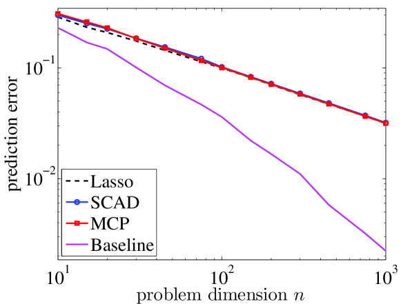
By varying the sample size over the range $10$ to $1000$, we obtained the results plotted in Figure 2, in which the prediction error $\mathbb{E}[\frac{1}{n}\|{X(\widehat{\theta}-\theta^{*})}\|_{2}^{2}]$ and sample size $n$ are both plotted on a logarithmic scale. The performance of the Lasso, SCAD-based estimate, and MCP-based estimate are all similar. For all of the three methods, the prediction error scales as $1/\sqrt{n}$, as confirmed by the slopes of the corresponding lines in Figure 2, which are very close to $0.5$. In fact, by examining the estimator’s output, we find that in many cases, all three estimators output $\widehat{\theta}=0$, leading to the prediction error $\frac{1}{n}\|{X(0-\theta^{*})}\|_{2}^{2}=\frac{1}{\sqrt{n}}$. Since the regularization parameters have been chosen to optimize the prediction error, this scaling is the best rate that the three estimators are able to achieve, and it matches the theoretical prediction of Theorem 1 and Theorem 2.

In contrast, the $\ell_{0}$-based estimator achieves a substantially better error rate. The slope of the corresponding line in Figure 2 is very close to $1$. It means that the prediction error of the $\ell_{0}$-based estimator scales as $1/n$, thereby matching the theoretically-predicted scaling (4).

4 Proofs

We now turn to the proofs of our theorems and corollary. In each case, we defer the proofs of more technical results to the appendices.

4.1 Proof of Theorem 1

For a given triple $(n,\sigma,R)$, we define the angle $\alpha:=\arcsin\left(\frac{\sqrt{\sigma}}{n^{1/4}\sqrt{32R}}\right)$, and the two-by-two matrix

$$A=\begin{bmatrix}\cos(\alpha)&-\cos(\alpha)\\ \sin(\alpha)&\sin(\alpha)\end{bmatrix}.$$ (21a)

Using the matrix $$A\in\mathbb{R}^{2\times 2} X\in\mathbb{R}^{n\times d} n n (n-1) d$$ as a building block, we construct a design matrix . Without loss of generality, we may assume that is divisible by two. (If is not divisible by two, constructing a -by- design matrix concatenated by a row of zeros only changes the result by a constant.) We then define

$$X=\Big{[}\mbox{blkdiag}\underbrace{\big{\{}\sqrt{n}A,\sqrt{n}A,\ldots,\sqrt{n}A\big{\}}}_{\mbox{$n/2$ copies}}~{}~{}{\bf 0}\Big{]}\in\mathbb{R}^{n\times d},$$ (21b)

where the all-zeroes matrix on the right side has dimensions $n\times(d-n)$. It is easy to verify that the matrix $X$ defined in this way satisfies the column normalization condition (10).

Next, we prove the lower bound (16a). For any integers $i,j\in[d]$ with $i<j$, let $\theta_{i}$ denote the $i^{th}$ coordinate of $\theta$, and let $\theta_{i:j}$ denote the subvector with entries $\{\theta_{i},\ldots,\theta_{j}\}$. Since the matrix $A$ appears in diagonal blocks of $X$, we have

$$\inf_{\lambda\geq 0}\sup_{\theta\in\widehat{\Theta}_{\lambda}}\frac{1}{n}\|X(\theta-\theta^{*})\|^{2}_{2} =\inf_{\lambda\geq 0}\sup_{\theta\in\widehat{\Theta}_{\lambda}}\sum_{i=1}^{n/2}\|{A\big{(}\theta_{(2i-1):2i}-\theta^{*}_{(2i-1):2i}\big{)}}\|_{2}^{2}$$ (22)

and it suffices to lower bound the right-hand side of the above equation.

For the sake of simplicity, we introduce the shorthand $B:=\frac{4\sigma}{\sqrt{n}}$, and define the scalars

$$\gamma_{i}=\min\{\rho_{2i-1}(B),\rho_{2i}(B)\}\qquad\mbox{for each $i=1,\ldots,n/2$.}$$ (23)

Furthermore, we define

$$a_{i}:=\left\{\begin{array}[]{ll}(\cos\alpha,\sin\alpha)&\mbox{if }\gamma_{i}=\rho_{2i-1}(B)\\ (-\cos\alpha,\sin\alpha)&\mbox{if }\gamma_{i}=\rho_{2i}(B)\end{array}\right.\quad\mbox{and}\quad w^{\prime}_{i}:=\frac{\langle a_{i},\,w_{(2i-1):2i}\rangle}{\sqrt{n}}.$$ (26)

Without loss of generality, we may assume that $\gamma_{1}=\max\limits_{i\in[n/2]}\{\gamma_{i}\}$ and $\gamma_{i}=\rho_{2i-1}(B)$ for all $i\in[n/2]$. If this condition does not hold, we can simply re-index the columns of $X$ to make these properties hold. Note that when we swap the columns $2i-1$ and $2i$, the value of $a_{i}$ doesn’t change; it is always associated with the column whose regularization term is equal to $\gamma_{i}$.

Finally, we define the regression vector $\theta^{*}=\begin{bmatrix}\frac{R}{2}&\frac{R}{2}&0&\cdots&0\end{bmatrix}\in\mathbb{R}^{d}$. Given these definitions, the following lemma lower bounds each term on the right-hand side of equation (22).

Lemma 1.

For any $\lambda\geq 0$, there is a local minimum $\widehat{\theta}_{\lambda}$ of the objective function $L(\theta;\lambda)$ such that $\frac{1}{n}\|X(\widehat{\theta}_{\lambda}-\theta^{*})\|^{2}_{2}\geq T_{1}+T_{2}$, where

$$T_{1} :=\mathbb{I}\Big{[}\lambda\gamma_{1}>4B(\sin^{2}(\alpha)R\frac{\|{w_{1:2}}\|_{2}}{\sqrt{n}})\Big{]}\sin^{2}(\alpha)(R-2B)_{+}^{2}\quad\mbox{and}$$ (27a)

$$T_{2} :=\sum_{i=2}^{n/2}\mathbb{I}\Big{[}B/2\leq w^{\prime}_{i}\leq B\Big{]}\Big{(}\frac{B^{2}}{4}-\lambda\gamma_{1}\Big{)}.$$ (27b)

Moreover, if the regularizer $\rho$ is convex, then every minimizer $\widehat{\theta}_{\lambda}$ satisfies this lower bound.

See Appendix B for the proof of this claim.

Using Lemma 1, we can now complete the proof of the theorem. It is convenient to condition on the event $\mathcal{E}:\,=\{\left\|{w_{1:2}}\right\|_{2}\leq\frac{\sigma}{32}\}$. Since $\left\|{w_{1:2}}\right\|_{2}^{2}/\sigma^{2}$ follows a chi-square distribution with two degrees of freedom, we have $\mathbb{P}[\mathcal{E}]>0$. Conditioned on this event, we now consider two separate cases:

Case 1:

First, suppose that $\lambda\gamma_{1}>\sigma^{2}/n$. In this case, we have

$$4B\Big{\{}\sin^{2}(\alpha)R+\frac{\|{w_{1:2}}\|_{2}}{\sqrt{n}}\Big{\}} \leq\frac{16\sigma}{\sqrt{n}}\left(\frac{\sigma}{32\sqrt{n}}+\frac{\sigma}{32\sqrt{n}}\right)=\frac{\sigma^{2}}{n}<\lambda\gamma_{1},$$

and consequently

$$T_{1}+T_{2}\geq T_{1}=\sin^{2}(\alpha)(R-2B)_{+}^{2}=\frac{\sigma}{32\sqrt{n}R}\left(R-\frac{4\sigma}{\sqrt{n}}\right)^{2}\geq\frac{\sigma R}{128\sqrt{n}},$$ (28a)

where the last inequality holds since we have assumed that $$R\geq 8\sigma/\sqrt{n}$$.

Case 2:

Otherwise, we may assume that $\lambda\gamma_{1}\leq\sigma^{2}/n$. In this case, we have

$$T_{1}+T_{2} \geq T_{2}=\sum_{i=2}^{n/2}\mathbb{I}\left(B/2\leq w^{\prime}_{i}\leq B\right)\frac{3\sigma^{2}}{n}.$$ (28b)

Combining the two lower bounds (28a) and (28b), we find

$$\mathbb{E}\left[\inf_{\lambda\geq 0}\sup_{\theta\in\widehat{\Theta}_{\lambda}}\frac{1}{n}\|{X\theta-X\theta^{*}}\|_{2}^{2}\Big{|}\mathcal{E}\right]$$

$$\qquad\geq\underbrace{\mathbb{E}\left[\min\left\{\frac{\sigma R}{128\sqrt{n}},\sum_{i=2}^{n/2}\mathbb{I}\left[B/2\leq w^{\prime}_{i}\leq B/2\right]\frac{3\sigma^{2}}{n}\right\}\right]}_{T_{3}},$$

where we have used the fact that $\{w^{\prime}_{i}\}_{i=2}^{n/2}$ are independent of the event $\mathcal{E}$. Using the inequality $\min\left\{a,\sum_{i=2}^{n/2}b_{i}\right\}\geq\sum_{i=2}^{n/2}\min\{2a/n,b_{i}\}$, valid for scalars $a$ and $\{b_{i}\}_{i=2}^{n/2}$, we see that

$$T_{3} \geq\sum_{i=2}^{n/2}\mathbb{P}\left[\frac{2\sigma}{\sqrt{n}}\leq w^{\prime}_{i}\leq\frac{4\sigma}{\sqrt{n}}\right]\min\left\{\frac{\sigma R}{128n\sqrt{n}},\frac{3\sigma^{2}}{n}\right\},$$

where we have used the fact that $\mathbb{E}\Big{[}\mathbb{I}\big{[}B/2\leq w^{\prime}_{i}\leq B\big{]}\Big{]}=\mathbb{P}[B/2\leq w^{\prime}_{i}\leq B]$, and the definition $B:=\frac{4\sigma}{\sqrt{n}}$.

Since $w^{\prime}_{i}\sim N(0,\sigma^{2}/n)$, the probability $\mathbb{P}[{2\sigma}/{\sqrt{n}}\leq w^{\prime}_{i}\leq{4\sigma}/{\sqrt{n}}]$ is bounded away from zero independently of all problem parameters. Hence, there is a universal constant $c_{2}>0$ such that $T_{3}\geq c_{2}\min\left\{\frac{\sigma R}{\sqrt{n}},\;\sigma^{2}\right\}$. Putting together the pieces, we have shown that

$$\mathbb{E}\left[\inf_{\lambda\geq 0}\sup_{\theta\in\widehat{\Theta}_{\lambda}}\frac{1}{n}\|{X\theta-X\theta^{*}}\|_{2}^{2}\right] \geq\>\mathbb{P}[\mathcal{E}]\,T_{3}\;\geq c_{2}^{\prime}\min\left\{\frac{\sigma R}{\sqrt{n}},\>\sigma^{2}\right\},$$

which completes the proof of the theorem.

4.2 Proof of Corollary 1

Here we provide a detailed proof of inequality (18a). We note that inequality (18b) follows by an essentially identical series of steps, so that we omit the details.

Let $m$ be an even integer and let $X_{m}\in{\mathbb{R}}^{m\times m}$ denote the design matrix constructed in the proof of Theorem 1. In order to avoid confusion, we rename the parameters $(n,d,R)$ in the construction (21b) by $(n^{\prime},d^{\prime},R^{\prime})$, and set them equal to

$$(n^{\prime},d^{\prime},R^{\prime}):=\Big{(}m,m,\min\Big{\{}\frac{R\sqrt{n}}{k\sqrt{m}},\frac{\sigma}{16\gamma\sqrt{m}}\Big{\}}\Big{)},$$ (29)

where the quantities $(k,m,n,R,\sigma)$ are defined in the statement of Corollary 1. Note that $X_{m}$ is a square matrix, and according to equation (21b), all of its eigenvalues are lower bounded by $(\frac{m^{1/2}\sigma}{16R^{\prime}})^{1/2}$. By equation (29), this quantity is lower bounded by $\sqrt{m\gamma}$.

Using the matrix $X_{m}$ as a building block, we now construct a larger design matrix $X\in{\mathbb{R}}^{n\times n}$ that we then use to prove the corollary. Let $m$ be the greatest integer divisible by two such that $km\leq n$. By the assumption that $n\geq 4k$, we have $m\geq 4$. Consequently, we may construct the $n\times n$ dimensional matrix

$$X:=\mbox{blkdiag}\Big{\{}\underbrace{\sqrt{n/m}X_{m},\ldots,\sqrt{n/m}X_{m}}_{\mbox{$k$ copies}},\sqrt{n}I_{n-km}\Big{\}}\in\mathbb{R}^{n\times n},$$ (30)

where $I_{n-km}$ is the $(n-km)$-dimensional identity matrix. It is easy to verify the matrix $X$ satisfies the column normalization condition. Since all eigenvalues of $X_{m}$ are lower bounded by $\sqrt{m\gamma}$, we are guaranteed that all eigenvalues of $X$ are lower bounded by $\sqrt{n\gamma}$. Thus, the matrix $X$ satisfies the $\gamma$-RE condition.

It remains to prove a lower bound on the prediction error, and in order to do so, it is helpful to introduce some shorthand notation. Given an arbitrary vector $u\in{\mathbb{R}}^{n}$, for each integer $i\in\{1,\ldots,k\}$, we let $u_{(i)}\in\mathbb{R}^{m}$ denote the sub-vector consisting of the $((i-1)m+1)$-th to the $(im)$-th elements of vector $u$, and we let $u_{(k+1)}$ denote the sub-vector consisting of the last $n-km$ elements. We also introduce similar notation for the function $\rho(x)=\rho_{1}(x_{1})+\dots+\rho_{n}(x_{n})$; specifically, for each $i\in\{1,\ldots,k\}$, we define the function $\rho_{(i)}:{\mathbb{R}}^{m}\to{\mathbb{R}}$ via $\rho_{(i)}(\theta):=\sum_{j=1}^{m}\rho_{(i-1)m+j}(\theta_{j})$.

Using this notation, we may rewrite the cost function as:

$$L(\theta;\lambda)=\frac{1}{n}\sum_{i=1}^{k}\Big{(}\|{\sqrt{n/m}X_{m}\theta_{(i)}-y_{(i)}}\|_{2}^{2}+n\lambda\rho_{(i)}(\theta_{(i)})\Big{)}+h(\theta_{(k+1)}),$$

where $h$ is a function that only depends on $\theta_{(k+1)}$. If we define $\theta^{\prime}_{(i)}:=\sqrt{n/m}\theta_{(i)}$ and $\rho^{\prime}_{(i)}(\theta):=\frac{n}{m}\rho_{(i)}(\sqrt{m/n}\theta)$, then substituting them into the above expression, the cost function can be rewritten as

$$G(\theta^{\prime};\lambda) :=\frac{m}{n}\sum_{i=1}^{k}\Big{(}\frac{1}{m}\|{X_{m}\theta^{\prime}_{(i)}-y_{(i)}}\|_{2}^{2}+\lambda\rho^{\prime}_{(i)}(\theta^{\prime}_{(i)})\Big{)}+h(\sqrt{m/n}\;\theta^{\prime}_{(k+1)}).$$

Note that if the vector $\widehat{\theta}$ is a local minimum of the function $\theta\mapsto L(\theta;\lambda)$, then the rescaled vector $\widehat{\theta}^{\prime}:=\sqrt{n/m}\;\widehat{\theta}$ is a local minimum of the function $\theta^{\prime}\mapsto G(\theta^{\prime};\lambda)$. Consequently, the sub-vector $\widehat{\theta}^{\prime}_{(i)}$ must be a local minimum of the function

$$\frac{1}{m}\|{X_{m}\theta^{\prime}_{(i)}-y_{(i)}}\|_{2}^{2}+\rho^{\prime}_{(i)}(\theta^{\prime}_{(i)}).$$ (31)

Thus, the sub-vector $\widehat{\theta}^{\prime}_{(i)}$ is the solution of a regularized sparse linear regression problem with design matrix $X_{m}$.

Defining the rescaled true regression vector $(\theta^{*})^{\prime}:=\sqrt{n/m}\;\theta^{*}$, we can then write the prediction error as

$$\frac{1}{n}\|{X(\widehat{\theta}-\theta^{*})}\|_{2}^{2} =\frac{1}{n}\sum_{i=1}^{k}\Big{(}\|{X_{m}(\widehat{\theta}^{\prime}_{(i)}-(\theta^{*})^{\prime}_{(i)})}\|_{2}^{2}\Big{)}+\|{\widehat{\theta}_{(k+1)}-\theta^{*}_{(k+1)}}\|_{2}^{2}$$

$$\geq\frac{m}{n}\sum_{i=1}^{k}\Big{(}\frac{1}{m}\|{X_{m}(\widehat{\theta}^{\prime}_{(i)}-(\theta^{*})^{\prime}_{(i)})}\|_{2}^{2}\Big{)}.$$ (32)

Consequently, the overall prediction error is lower bounded by a scaled sum of the prediction errors associated with the design matrix $X_{m}$. Moreover, each term $\frac{1}{m}\|{X_{m}(\widehat{\theta}^{\prime}_{(i)}-(\theta^{*})^{\prime}_{(i)})}\|_{2}^{2}$ can be bounded by Theorem 1.

More precisely, let $\mathcal{Q}(X,2k,R)$ denote the left-hand side of inequality (18a). The above analysis shows that the sparse linear regression problem on the design matrix $X$ and the constraint $\theta^{*}\in\mathbb{B}_{0}(2k)\cap\mathbb{B}_{1}(R)$ can be decomposed into smaller-scale problems on the design matrix $X_{m}$ and constraints on the scaled vector $(\theta^{*})^{\prime}$. By the rescaled definition of $(\theta^{*})^{\prime}$, the constraint $\theta^{*}\in\mathbb{B}_{0}(2k)\cap\mathbb{B}_{1}(R)$ holds if and only if $(\theta^{*})^{\prime}\in\mathbb{B}_{0}(2k)\cap\mathbb{B}_{1}(\sqrt{n/m}R)$. Recalling the definition of the radius $R^{\prime}$ from equation (29), we can ensure that $(\theta^{*})^{\prime}\in\mathbb{B}_{0}(2k)\cap\mathbb{B}_{1}(\sqrt{n/m}R)$ by requiring that $(\theta^{*})^{\prime}_{(i)}\in\mathbb{B}_{0}(2)\cap\mathbb{B}_{1}(R^{\prime})$ for each index $i\in\{1,\dots,k\}$. Combining expressions (31) and (32), the quantity $\mathcal{Q}(X,2k,R)$ can be lower bounded by the sum

$$\mathcal{Q}(X,2k,R)\geq\frac{m}{n}\sum_{i=1}^{k}\mathcal{Q}(X_{m},2,R^{\prime}).$$ (33a)

By Theorem 1, we have

$$\mathcal{Q}(X_{m},2,R^{\prime})\geq c\min\left\{\sigma^{2},\frac{\sigma R^{\prime}}{\sqrt{m}}\right\}=c\min\left\{\sigma^{2},\frac{\sigma^{2}}{16\gamma m},\frac{\sigma R\sqrt{n}}{km}\right\},$$ (33b)

where the second equality follows from our choce of $R^{\prime}$ from equation (29). Combining the lower bounds (33a) and (33b) completes the proof.

4.3 Proof of Theorem 2

The proof of Theorem 2 is conceptually similar to the proof of Theorem 1, but differs in some key details. We begin with the altered definitions

$$\alpha:=\arcsin\left(\frac{\sqrt{\sigma}}{n^{1/4}\sqrt{r}}\right)\quad\mbox{and}\quad B:=\frac{\sigma}{4\sqrt{n}},\qquad\mbox{where }r:=\min\{R,\sigma\}.$$

Given our assumption $R\geq\sigma/\sqrt{n}$, note that we are guaranteed that the inequality $2B=\sigma/(2\sqrt{n})\leq r/2$ holds. We then define the matrix $A\in{\mathbb{R}}^{2\times 2}$ and the matrix $X\in{\mathbb{R}}^{n\times d}$ by equations (21a) and (21b).

4.3.1 Proof of part (a)

Let $\{\theta^{t}\}_{t=0}^{\infty}$ be the sequence of iterates generated by equation (19). We proceed via proof by contradiction, assuming that the sequence does not terminate finitely, and then deriving a contradiction. We begin with a lemma.

Lemma 2.

If the sequence of iterates $\{\theta^{t}\}_{t=0}^{\infty}$ is not finitely convergent, then it is unbounded.

We defer the proof of this claim to the end of this section. Based on Lemma 2, it suffices to show that, in fact, the sequence $\{\theta^{t}\}_{t=0}^{\infty}$ is bounded. Partitioning the full vector as $\theta:=\big{(}\theta_{1:n},\theta_{n+1:d}\big{)}$, we control the two sequences $\{\theta^{t}_{1:n}\}_{t=0}^{\infty}$ and $\{\theta^{t}_{n+1:d}\}_{t=0}^{\infty}$.

Beginning with the former sequence, notice that the objective function can be written in the form

$$L(\theta;\lambda)=\frac{1}{n}\|{y-X_{1:n}\theta_{1:n}}\|_{2}^{2}+\sum_{i=1}^{d}\lambda\rho_{i}(\theta_{i}),$$

where $X_{1:n}$ represents the first $n$ columns of matrix $X$. The conditions (21a) and (21b) guarantee that the Gram matrix $X_{1:n}^{T}X_{1:n}$ is positive definite, which implies that the quadratic function $\theta_{1:n}\mapsto\|{y-X_{1:n}\theta_{1:n}}\|_{2}^{2}$ is strongly convex. Thus, if the sequence $\{\theta_{1:n}^{t}\}_{t=0}^{\infty}$ were unbounded, then the associated cost sequence $\{L(\theta^{t};\lambda)\}_{t=0}^{\infty}$ would also be unbounded. But this is not possible since $L(\theta^{t};\lambda)\leq L(\theta^{0};\lambda)$ for all iterations $t=1,2,\ldots$. Consequently, we are guaranteed that the sequence $\{\theta^{t}_{1:n}\}_{t=0}^{\infty}$ must be bounded.

It remains to control the sequence $\{\theta_{n+1:d}^{t}\}_{t=0}^{\infty}$. We claim that for any $i\in\{n+1,\ldots,d\}$, the sequence $\{|\theta_{i}^{t}|\}_{t=0}^{\infty}$ is non-increasing, which implies the boundedness condition. Proceeding via proof by contradiction, suppose that $|\theta^{t}_{i}|<|\theta^{t+1}_{i}|$ for some index $i\in\{n+1,\ldots,d\}$ and iteration number $t\geq 0$. Under this condition, define the vector

$$\widetilde{\theta}^{t+1}_{j}:=\begin{cases}\theta^{t+1}_{j}&\mbox{if $j\neq i$}\\ \theta^{t}_{j}&\mbox{if $j=i$.}\end{cases}$$

Since $\rho_{j}$ is a monotonically non-decreasing function of $|x|$, we are guaranteed that $L(\widetilde{\theta}^{t+1};\lambda)\leq L(\theta^{t+1};\lambda)$, which implies that $\widetilde{\theta}^{t+1}$ is also a constrained minimum point over the ball $\mathbb{B}_{2}(\eta;\theta^{t})$. In addition, we have

$$\|{\widetilde{\theta}^{t+1}-\theta^{t}}\|_{2}=\|{\theta^{t+1}-\theta^{t}}\|_{2}-|\theta^{t}_{i}-\theta^{t+1}_{i}|<\eta,$$

so that $\widetilde{\theta}^{t+1}_{j}$ is strictly closer to $\theta^{t}$. This contradicts the specification of the algorithm, in that it chooses the minimum closest to $\theta^{t}$.

Proof of Lemma 2:

The final remaining step is to prove Lemma 2. We first claim that $\|{\theta^{s}-\theta^{t}}\|_{2}\geq\eta$ for all pairs $s<t$. If not, we could find some pair $s<t$ such that $\|{\theta^{s}-\theta^{t}}\|_{2}<\eta$. But since $t>s$, we are guaranteed that $L(\theta^{t};\lambda)\leq L(\theta^{s+1};\lambda)$. Since $\theta^{s+1}$ is a global minimum over the ball $\mathbb{B}_{2}(\eta;\theta^{s})$ and $\|{\theta^{s}-\theta^{t}}\|_{2}<\eta$, the point $\theta^{t}$ is also a global minimum, and this contradicts the definition of the algorithm (since it always chooses the constrained global minimum closest to the current iterate).

Using this property, we now show that $\{\theta^{t}\}_{t=0}^{\infty}$ is unbounded. For each iteration $t=0,1,2\ldots$, we use $\mathbb{B}^{t}=\mathbb{B}_{2}(\eta/3;\theta^{t})$ to denote the Euclidean ball of radius $\eta/3$ centered at $\theta^{t}$. Since $\|{\theta^{s}-\theta^{t}}\|_{2}\geq\eta$ for all $s\neq t$, the balls $\{\mathbb{B}^{t}\}_{t=0}^{\infty}$ are all disjoint, and hence there is a numerical constant $C>0$ such that for each $T\geq 1$, we have

$${\rm vol}\Big{(}\cup_{t=0}^{T}\mathbb{B}^{t}\Big{)}=\sum_{t=0}^{T}{\rm vol}(\mathbb{B}^{t})=C\sum_{t=0}^{T}\eta^{d}.$$

Since this volume diverges as $T\rightarrow\infty$, we conclude that the set $\mathbb{B}:\,=\cup_{t=0}^{\infty}\mathbb{B}^{t}$ must be unbounded. By construction, any point in $\mathbb{B}$ is within $\eta/3$ of some element of the sequence $\{\theta^{t}\}_{t=0}^{\infty}$, so this sequence must be unbounded, as claimed.

4.3.2 Proof of part (b)

We now prove a lower bound on the prediction error corresponding the local minimum to which the algorithm converges, as claimed in part (b) of the theorem statement. In order to do so, we begin by introducing the shorthand notation

$$\gamma_{i}=\min\{\sup_{u\in(0,B]}\rho^{\prime}_{2i-1}(u),\sup_{u\in(0,B]}\rho^{\prime}_{2i}(u)\}\qquad\mbox{for each $i=1,\ldots,n/2$}.$$ (34)

Then we define the quantities $a_{i}$ and $w^{\prime}_{i}$ by equations (26). Similar to the proof of Theorem 1, we assume (without loss of generality, re-indexing as needed) that $\gamma_{i}=\sup_{u\in(0,B]}\rho^{\prime}_{2i-1}(u)$ and that $\gamma_{1}=\max_{i\in[n/2]}\{\gamma_{i}\}$.

Consider the regression vector $\theta^{*}:\,=\begin{bmatrix}\frac{r}{2}&\frac{r}{2}&0&\cdots&0\end{bmatrix}$. Since the matrix $A$ appears in diagonal blocks of $X$, the algorithm’s output $\widehat{\theta}$ has error

$$\inf_{\lambda\geq 0}\frac{1}{n}\|X(\widehat{\theta}-\theta^{*})\|^{2}_{2} =\inf_{\lambda\geq 0}\sum_{i=1}^{n/2}\|{A\big{(}\widehat{\theta}_{(2i-1):2i}-\theta^{*}_{(2i-1):2i}\big{)}}\|_{2}^{2}.$$ (35)

Given the random initialization $\theta^{0}$, we define the events

$$\mathcal{E}_{0}:=\Big{\{}\max\{\theta_{1}^{0},\theta_{2}^{0}\}\leq 0\Big{\}}\quad\mbox{and}\quad\mathcal{E}_{1}:=\Big{\{}\lambda\gamma_{1}\geq 2\sin^{2}(\alpha)r+\frac{2\|{w_{1:2}}\|_{2}}{\sqrt{n}}+3B\Big{\}},$$

as well as the (random) subsets

$$\mathbb{S}_{1} :=\Big{\{}i\in\big{\{}2,\ldots,n/2\big{\}}\,\mid\,\lambda\gamma_{1}\leq 2w^{\prime}_{i}-4B\Big{\}},\quad\mbox{and}$$

$$\mathbb{S}_{2} :=\Big{\{}i\in\{2,\ldots,n/2\}\,\mid\,\mbox{$2\sin^{2}(\alpha)r+\frac{2\|{w_{1:2}}\|_{2}}{\sqrt{n}}+3B\leq 2w^{\prime}_{i}-4B$}\Big{\}}.$$

Here the reader should recall the definition of $w^{\prime}$ from equation (26).

Given these definitions, the following lemma provides lower bounds on the decomposition (35) for the vector $\widehat{\theta}$ after convergence.

Lemma 3.

1. If $\mathcal{E}_{0}\cap\mathcal{E}_{1}$ holds, then $\|{A\,\big{(}\widehat{\theta}_{1:2}-\theta^{*}_{1:2}\big{)}}\|_{2}^{2}\geq\frac{\sigma r}{4\sqrt{n}}$.

2. For any index $i\in\mathbb{S}_{1}$, we have $\|{A\,\big{(}\widehat{\theta}_{2i-1:2i}-\theta^{*}_{2i-1:2i}\big{)}}\|_{2}^{2}\geq\frac{\sigma r}{8n^{3/2}}$.

3. We have $\mathbb{P}[\mathcal{E}_{0}]=1/4$, and moreover $\min\limits_{i\in\{2,\ldots,n/2\}}\mathbb{P}[i\in\mathbb{S}_{2}]\geq c$ for some numerical constant $c>0$.

See Appendix C for the proof of this claim.

Conditioned on event $\mathcal{E}_{0}$, for any index $i\in\mathbb{S}_{2}$, either the event $\mathcal{E}_{0}\cap\mathcal{E}_{1}$ holds, or we have

$$\lambda\gamma_{1}<2\sin^{2}(\alpha)r+\frac{2\|{w_{1:2}}\|_{2}}{\sqrt{n}}+3B\leq 2w^{\prime}_{i}-4B,$$

which means that $i\in\mathbb{S}_{1}$ holds. Applying Lemma 3 yields the lower bound

$$\inf_{\lambda\geq 0}\sum_{i=1}^{n/2}\|{A\widehat{\theta}_{(2i-1):2i}-A\theta^{*}_{(2i-1):2i}}\|_{2}^{2} \geq\mathbb{I}[\mathcal{E}_{0}]\;\min\left\{\frac{\sigma r}{4\sqrt{n}},\>\;\frac{\sigma r}{8n^{3/2}}\;\sum_{i=2}^{[n/2]}\mathbb{I}[i\in\mathbb{S}_{2}]\right\}$$

$$=\mathbb{I}[\mathcal{E}_{0}]\;\frac{\sigma r}{8n^{3/2}}\;\sum_{i=2}^{[n/2]}\mathbb{I}[i\in\mathbb{S}_{2}],$$

where the last equality holds since $\frac{\sigma r}{8n^{3/2}}\;\sum_{i=2}^{[n/2]}\mathbb{I}[i\in\mathbb{S}_{2}]\leq\frac{\sigma r}{8n^{3/2}}\;(n/2-1)<\frac{\sigma r}{4\sqrt{n}}$. Since the event $\mathcal{E}_{0}$ is independent of the event $\{i\in\mathbb{S}_{2},i=2,\ldots,n/2\}$, we have

$$\mathbb{E}\Big{[}\inf_{\lambda\geq 0}\sum_{i=1}^{n/2}\|{A\widehat{\theta}_{(2i-1):2i}-A\theta^{*}_{(2i-1):2i}}\|_{2}^{2}\Big{]} \geq\mathbb{P}[\mathcal{E}_{0}]\;\frac{\sigma r}{8n^{3/2}}\sum_{i=2}^{[n/2]}\mathbb{P}[i\in\mathbb{S}_{2}]$$

$$\stackrel{{\scriptstyle(i)}}{{\geq}}\frac{1}{4}\;\frac{\sigma r}{8n^{3/2}}\;c(n/2-1)$$

$$=c^{\prime}\min\{R,\sigma\}\,\frac{\sigma}{\sqrt{n}},$$

where step (i) uses the lower bound $\mathbb{P}[\mathcal{E}_{0}]=1/4$ and $\mathbb{P}[i\in\mathbb{S}_{2}]\geq c$ from Lemma 3. Combined with the decomposition (35), the proof is complete.

5 Discussion

In this paper, we have demonstrated a fundamental gap in sparse linear regression: the best prediction risk achieved by a class of $M$-estimators based on coordinate-wise separable regularizers is strictly larger than the the classical minimax prediction risk, achieved for instance by minimization over the $\ell_{0}$-ball. This gap applies to a range of methods used in practice, including the Lasso in its ordinary and weighted forms, as well as estimators based on nonconvex penalties such as the MCP and SCAD penalties.

Several open questions remain, and we discuss a few of them here. When the penalty function $\rho$ is convex, the M-estimator minimizing function (9) can be understood as a particular convex relaxation of the $\ell_{0}$-based estimator (3). It would be interesting to consider other forms of convex relaxations for the $\ell_{0}$-based problem. For instance, Pilanci et al. [27] show how a broad class of $\ell_{0}$-regularized problems can be reformulated exactly as optimization problems involving convex functions in Boolean variables. This exact reformulation allows for the direct application of many standard hierarchies for Boolean polynomial programming, including the Lasserre hierarchy [21] as well as the Sherali-Adams hierarchy [29]. Other relaxations are possible, including those that are based on introducing auxiliary variables for the pairwise interactions (e.g., $\gamma_{ij}=\theta_{i}\theta_{j}$), and so incorporating these constraints as polynomials in the constraint set. We conjecture that for any fixed natural number $t$, if the the $t$-th level Lasserre (or Sherali-Adams) relaxation is applied to such a reformulation, it still does not yield an estimator that achieves the fast rate (4). Since a $t^{th}$-level relaxation involves $\mathcal{O}(d^{t})$ variables, this would imply that these hierarchies do not contain polynomial-time algorithms that achieve the classical minimax risk. Proving or disproving this conjecture remains an open problem.

Finally, when the penalty function $\rho$ is concave, concurrent work by Ge et al. [17] shows that finding the global minimum of the loss function (9) is strongly NP-hard. This result implies that no polynomial-time algorithm computes the global minimum unless ${\bf NP}={\bf P}$. The result given here is complementary in nature: it shows that bad local minima exist, and that local descent methods converge to these bad local minima. It would be interesting to extend this algorithmic lower bound to a broader class of first-order methods. For instance, we suspect that any algorithm that relies on an oracle giving first-order information will inevitably converge to a bad local minimum for a broad class of random initializations.

Acknowledgements

This work was partially supported by grants NSF grant DMS-1107000, NSF grant CIF-31712-23800, Air Force Office of Scientific Research Grant AFOSR-FA9550-14-1-0016, and Office of Naval Research MURI N00014-11-1-0688.

Appendix A Fast rate for the bad example of Dalalyan et al. [12]

In this appendix, we describe the bad example of Dalayan et al. [12], and show that a reweighted form of the Lasso achieves the fast rate. For a given sample size $n\geq 4$, they consider a linear regression model $y=X\theta^{*}+w$, where $X\in\mathbb{R}^{n\times 2m}$ with $m=n-1$, and the noise vector $w\in\{-1,1\}^{n}$ has i.i.d. Rademacher entries (equiprobably chosen in $\{-1,1\}$). In the construction, the true vector $\theta^{*}$ is 2-sparse, and the design matrix $X\in{\mathbb{R}}^{n\times 2m}$ is given by

$$X=\sqrt{n}\begin{bmatrix}{\bf 1}^{T}_{m}&{\bf 1}^{T}_{m}\\ I_{m\times m}&-I_{m\times m}\end{bmatrix}$$

where ${\bf 1}_{m}\in\mathbb{R}^{m}$ is a vector of all ones. Notice that this construction has $n=m+1$.

In this appendix, we analyze the performance of the following estimator

$$\widehat{\theta}\in\arg\min_{\theta\in{\mathbb{R}}^{2m}}\frac{1}{n}\|{X\theta-y}\|_{2}^{2}+\lambda\sum_{i=2}^{m}(|\theta_{i}|+|\theta_{m+i}|).$$ (36)

It is a reweighted form of the Lasso based on $\ell_{1}$-norm regularization, but one that imposes no constraint on the first and the $(m+1)$-th coordinate. We claim that with an appropriate choice of $\lambda$, this estimator achieves the fast rate for any $2$-sparse vector $\theta^{*}$.

Letting $\widehat{\theta}$ be a minimizer of function (36), we first observe that no matter what value it attains, the minimizer always chooses $\widehat{\theta}_{1}$ and $\widehat{\theta}_{m+1}$ so that $(X\widehat{\theta})_{1:2}=y_{1:2}$. This property occurs because:

• There is no penalty term associated with $\widehat{\theta}_{1}$ and $\widehat{\theta}_{m+1}$.

• By the definition of $X$, changes in the coordinates $\widehat{\theta}_{1}$ and $\widehat{\theta}_{m+1}$ only affect the first two coordinates of $X\widehat{\theta}$ by the additive term

  $$\sqrt{n}\begin{bmatrix}1&1\\ e_{1}&-e_{1}\end{bmatrix}\cdot\begin{bmatrix}\widehat{\theta}_{1}\\ \widehat{\theta}_{m+1}\end{bmatrix}$$

  Since the above 2-by-2 matrix is non-singular, there is always an assignment to $(\widehat{\theta}_{1},\widehat{\theta}_{m+1})$ so that $(X\widehat{\theta})_{1:2}-y_{1:2}=0$.

Thus, only the last $n-2$ coordinates of $X\widehat{\theta}-y$ might be non-zero, so that we may rewrite the objective function (36) as

$$\frac{1}{n}\|{X\widehat{\theta}-y}\|_{2}^{2}+\lambda\sum_{i=2}^{m}(|\widehat{\theta}_{i}|+|\widehat{\theta}_{m+i}|)$$

$$\qquad=\frac{1}{n}\sum_{i=2}^{m}\left((\sqrt{n}\widehat{\theta}_{i}-\sqrt{n}\widehat{\theta}_{m+i}-y_{i})^{2}+\lambda(|\widehat{\theta}_{i}|+|\widehat{\theta}_{m+i}|)\right)$$ (37)

The function (A) is not strictly convex so that there are multiple equivalent solutions. Essentially, we need to break symmetry by choosing to vary one of $\widehat{\theta}_{i}$ or $\widehat{\theta}_{m+i}$, for each $i\in\{2,\ldots,m\}$. Without loss of generality, we assume that $\widehat{\theta}_{m+2}=\widehat{\theta}_{m+3}=\dots=\widehat{\theta}_{2m}=0$, so that the equation is simplified as

$$\frac{1}{n}\|{X\widehat{\theta}-y}\|_{2}^{2}+\lambda\sum_{i=2}^{m}(|\widehat{\theta}_{i}|+|\widehat{\theta}_{m+i}|)=\frac{1}{n}\sum_{i=2}^{m}\left((\sqrt{n}\widehat{\theta}_{i}-y_{i})^{2}+\lambda|\widehat{\theta}_{i}|)\right).$$ (38)

Moreover, with this choice, we can write the prediction error as

$$R(\widehat{\theta}):=\frac{1}{n}\|{X\widehat{\theta}-X\theta^{*}}\|_{2}^{2}=\frac{2}{n}+\frac{1}{n}\sum_{i=2}^{m}(\sqrt{n}\widehat{\theta}_{i}-\sqrt{n}(\theta^{*}_{i}-\theta^{*}_{m+i}))^{2}.$$ (39)

The first term on the right-hand side is obtained from the fact $\|{(X\widehat{\theta}-X\theta^{*})_{1:2}}\|_{2}^{2}=\|{w_{1:2}}\|_{2}^{2}=2$, recalling that the set-up assumes that the noise elements takes values in $\{-1,1\}$.

The right-hand side of equation (38) is a Lasso objective function with design matrix $\sqrt{n}I_{(m-1)\times(m-1)}$. The second term on the right-hand side of equation (39) is the associated prediction error. By choosing a proper $\lambda$ and using the fact that $\theta^{*}$ is 2-sparse, it is well-known that the prediction error scales as $\mathcal{O}(\frac{\log n}{n})$, which corresponds the fast rate. (Here we have recalled that the dimension of the Lasso problem is $m-1=n-2$.)

Appendix B Proof of Lemma 1

Given our definition of $X$ in terms of the matrix $A\in\mathbb{R}^{2\times 2}$, it suffices to prove the two lower bounds

$$\|{A(\widehat{\theta}_{\lambda})_{1:2}-A\theta^{*}_{1:2}}\|_{2}^{2}$$ (40a)

$$\qquad\geq\mathbb{I}\Big{[}\lambda\gamma_{1}>4B(\sin^{2}(\alpha)R+\frac{\|{w_{1:2}}\|_{2}}{\sqrt{n}})\Big{]}\sin^{2}(\alpha)(R-2B)_{+}^{2}\quad\mbox{and},$$

$$\|{A(\widehat{\theta}_{\lambda})_{2i-1:2i}-A\theta^{*}_{2i-1:2i}}\|_{2}^{2}$$ (40b)

$$\qquad\geq\mathbb{I}\Big{[}0\leq w^{\prime}_{i}\leq B\Big{]}(\frac{B^{2}}{4}-\lambda\gamma_{1})\quad\mbox{for $i=2,3,\ldots,n/2$.}$$

In the proofs to follow, it is convenient to omit reference to the index $i$. In particular, viewing the index $i$ as fixed a priori, we let $\widehat{u}$ and $u^{*}$ be shorthand representations of the sub-vectors $(\widehat{\theta}_{\lambda})_{2i-1,2i}$, and $\theta^{*}_{2i-1,2i}$, respectively. We introduce the normalized noise $\varepsilon:=w_{2i-1,2i}/\sqrt{n}$. By our construction of the design matrix $X$ in terms of $A$, the vector $\widehat{\theta}_{\lambda}$ is a local minimizer of the objective function if and only if $\widehat{u}$ is a local minimum of the following loss:

$$\ell(u;\lambda):=\|{Au-Au^{*}-\varepsilon}\|_{2}^{2}+\lambda\rho_{2i-1}(u_{1})+\lambda\rho_{2i}(u_{2}),$$

where this statement should hold for each $i\in[n/2]$. Hence, it suffices to find a local minimum of $\ell(u;\lambda)$ such that the bounds (40a) and (40b) hold.

B.1 Proof of inequality (40a)

If $\lambda\gamma_{1}\leq 4B(\sin^{2}(\alpha)R+\|{\varepsilon}\|_{2})$, then the lower bound (40a) is trivial, and in particular, it will hold for

$$\widehat{u}:=\arg\min_{u}\ell(u;\lambda).$$

Otherwise, we may assume that $\lambda\gamma_{1}>4B(\sin^{2}(\alpha)R+\|{\varepsilon}\|_{2})$. In this case ($i=1$), we have $u^{*}=(R/2,R/2)$. Defining the vectors $v^{*}:=Au^{*}=(0,\sin(\alpha)R)$ and $\widetilde{u}:=(0,0)$, we have

$$\ell(\widetilde{u};\lambda) =\|{A\widetilde{u}-v^{*}-\varepsilon}\|_{2}^{2}+\lambda\rho_{1}(\widetilde{u}_{1})+\lambda\rho_{2}(\widetilde{u}_{2})=\|{v^{*}+\varepsilon}\|_{2}^{2}.$$ (41)

We claim that

$$\inf_{u\in\partial U}\ell(u;\lambda)>\ell(\widetilde{u};\lambda),$$ (42)

where $U:=\{u\in\mathbb{R}^{2}\,\mid\,|u_{1}|\leq B\mbox{ or }|u_{2}|\leq B\}$, and $\partial U$ denotes its boundary. If $\rho$ is a convex function, then the lower bound (42) implies that any minimizers of the function $\ell(\cdot;\lambda)$ lie in the interior of $U$. Otherwise, it implies that at least one local minimum—say $\widehat{u}$—lies in the interior of $U$. Since $\widehat{u}_{1}\leq B$ and $\widehat{u}_{2}\leq B$, we have the lower bound

$$\|{A(\widehat{\theta}_{\lambda})_{1:2}-A\theta^{*}_{1:2}}\|_{2}^{2} =\|{A\widehat{u}-v^{*}}\|_{2}=\cos^{2}(\alpha)(\widehat{u}_{1}-\widehat{u}_{2})^{2}+\sin^{2}(\alpha)(R-\widehat{u}_{1}-\widehat{u}_{2})^{2}$$

$$\geq\sin^{2}(\alpha)(R-\widehat{u}_{1}-\widehat{u}_{2})^{2}\geq\sin^{2}(\alpha)(R-2B)_{+}^{2},$$

which completes the proof.

It remains to prove the lower bound (42). For any $u\in\partial U$, we have

$$\ell(u;\lambda) =\|{Au-v^{*}-\varepsilon}\|_{2}^{2}+\lambda\rho_{1}(\widetilde{u}_{1})+\lambda\rho_{2}(\widetilde{u}_{2})\stackrel{{\scriptstyle(i)}}{{\geq}}\|{Au+v^{*}+\varepsilon}\|_{2}^{2}+\lambda\gamma_{1}$$

$$\stackrel{{\scriptstyle(ii)}}{{\geq}}\|{v^{*}+\varepsilon}\|_{2}^{2}+2(v^{*}+\varepsilon)^{T}Au+\lambda\gamma_{1}.$$ (43)

Inequality (i) holds since either $\widetilde{u}_{1}$ or $\widetilde{u}_{2}$ is equal to $B$, and $\min\{\rho_{1}(B),\rho_{2}(B)\}\geq\gamma_{1}$ by definition, whereas inequality (ii) holds since $\|{a+b}\|_{2}^{2}\geq\|{b}\|_{2}^{2}+2b^{T}a$. We notice that

$$\inf_{u\in\partial U}2(v^{*}+\varepsilon)^{T}Au\geq\inf_{u\in\partial U}\left\{2\langle v^{*},Au\rangle-2\|{\varepsilon}\|_{2}\left\|{Au}\right\|_{2}\right\}$$

$$\qquad=\inf_{u\in\partial U}\left\{2\sin^{2}(\alpha)R(u_{1}+u_{2})-2\|{\varepsilon}\|_{2}\sqrt{\cos^{2}(\alpha)(u_{1}+u_{2})^{2}+\sin^{2}(\alpha)(u_{1}-u_{2})^{2}}\right\}$$

$$\qquad\geq-4B(\sin^{2}(\alpha)R+\|{\varepsilon}\|_{2}).$$

Combining this lower bound with inequality (B.1) and the bound $\lambda\gamma_{1}>4B(\sin^{2}(\alpha)R+\|{\varepsilon}\|_{2})$ yields the claim (42).

B.2 Proof of inequality (40b)

For $i=2,3,\dots,n/2$, consider $u^{*}=(0,0)$ and recall the vector $a_{i}=(\cos\alpha,\sin\alpha)$, as well as our assumption that

$$\gamma_{i}:=\rho_{2i-1}(B)/B\leq\frac{\rho_{2i}(B)}{B}.$$

Define the vector $\widetilde{u}:=(a_{i}^{T}\varepsilon,0)$ and let $\widehat{u}=\arg\min_{u\in\mathbb{R}^{2}}\ell(u;\lambda)$ be an arbitrary global minimizer. We then have

$$\|{A\widehat{u}-\varepsilon}\|_{2}^{2} \leq\|{A\widehat{u}-\varepsilon}\|_{2}^{2}+\lambda\rho_{1}(\widehat{u}_{1})+\lambda\rho_{2}(\widehat{u}_{2})\leq\|{A\widetilde{u}-\varepsilon}\|_{2}^{2}+\lambda\rho_{1}(\widetilde{u}_{1})+\lambda\rho_{2}(\widetilde{u}_{2}),$$

since the regularizer is non-negative, and $\widehat{u}$ is a global minimum. Using the definition of $\widetilde{u}$, we find that

$$\|{A\widehat{u}-\varepsilon}\|_{2}^{2} \leq\|{a_{i}a_{i}^{T}\varepsilon-\varepsilon}\|_{2}^{2}+\lambda\rho_{1}(a_{i}^{T}\varepsilon)=\|{\varepsilon}\|_{2}^{2}-(a_{i}^{T}\varepsilon)^{2}+\lambda\rho_{1}(a_{i}^{T}\varepsilon),$$

where the final equality holds since $a_{i}a_{i}^{T}$ defines an orthogonal projection. By the triangle inequality, we find that $\|{A\widehat{u}-\varepsilon}\|_{2}^{2}\geq\|{\varepsilon}\|_{2}^{2}-\|{A\widehat{u}}\|_{2}^{2}$, and combining with the previous inequality yields

$$\|{A\widehat{u}}\|_{2}^{2}\geq(a_{i}^{T}\varepsilon)^{2}-\lambda\rho_{1}(a_{i}^{T}\varepsilon).$$ (44)

Now if $B/2\leq a^{T}\varepsilon\leq B$, then we have $\rho_{1}(a_{i}^{T}\varepsilon)\leq\rho_{1}(B)=\gamma_{i}\leq\gamma_{1}$. Substituting this relation into inequality (44), we have $\|{A\widehat{u}-\varepsilon}\|_{2}^{2}\geq\mathbb{I}(B/2\leq a_{i}^{T}\varepsilon\leq B)\left(B^{2}/4-\lambda\gamma_{1}\right)$, which completes the proof.

Appendix C Proof of Lemma 3

Similar to the proof of Lemma 1, it is convenient to omit reference to the index $i$. We let $u^{t}$ and $u^{*}$ be shorthand representations of the sub-vectors $u^{t}_{2i-1,2i}$, and $\theta^{*}_{2i-1,2i}$, respectively. We introduce the normalized noise $\varepsilon:=w_{2i-1,2i}/\sqrt{n}$. By our construction of the design matrix $X$ and the update formula (19), the vector $u^{t}$ satisfies the recursion

$$u^{t+1}\in\underset{\|{u-u^{t}}\|_{2}\leq\beta}{{\rm argmin}}\ell(u;\lambda),$$ (45a)

where $$\beta:=\|{u^{t+1}-u^{t}}\|_{2}\leq\eta$$ and the loss function takes the form

$$\ell(u;\lambda):=\underbrace{\|{Au-Au^{*}-\varepsilon}\|_{2}^{2}}_{:=T}+\lambda\rho_{2i-1}(u_{1})+\lambda\rho_{2i}(u_{2}).$$ (45b)

This statement holds for each $i\in[n/2]$. Hence, it suffices to study the update formula (45a).

C.1 Proof of part (a)

For the case of $i=1$, we assume that the event $\mathcal{E}_{2}$ holds. Consequently, we have $\max\{u^{0}_{1},u^{0}_{2}\}\leq 0$ and $\lambda\gamma_{1}\geq 2\sin^{2}(\alpha)r+2\|{\varepsilon}\|_{2}$. The corresponding regression vector is $u^{*}=(r/2,r/2)$. Let us define

$$b_{1}\in\arg\sup_{u\in(0,B]}\rho_{2i-1}(u)\quad\mbox{and}\quad b_{2}\in\arg\sup_{u\in(0,B]}\rho_{2i}(u).$$

Our assumption implies $\rho^{\prime}_{2i-1}(b_{1})\geq\gamma_{1}$ and $\rho^{\prime}_{2i}(b_{2})\geq\gamma_{1}$. We claim that

$$u^{t}_{k}\leq b_{k}\leq B\quad\mbox{for $k=1,2$ and for all iterations $t=0,1,2,\ldots$.}$$ (46)

If the claim is true, then we have

$$\|{A\theta^{t}_{1:2}-A\theta^{*}_{1:2}}\|_{2}^{2} =\cos^{2}(\alpha)(u^{t}_{1}-u^{t}_{2})^{2}+\sin^{2}(\alpha)(r-u^{t}_{1}-u^{t}_{2})^{2}$$

$$\geq\sin^{2}(\alpha)(r-u^{t}_{1}-u^{t}_{2})^{2}\geq\sin^{2}(\alpha)(r-2B)_{+}^{2}$$

$$\geq\frac{\sigma r}{4\sqrt{n}},$$

where the final inequality follows from substituting the definition of $\alpha$, and using the fact that $2B\leq r/2$. Thus, it suffices to prove the claim (46).

We prove the claim (46) by induction on the iteration number $t$. It is clearly true for $t=0$. Assume that the claim is true for a specific integer $t\geq 0$, we establish it for integer $t+1$. Our strategy is as follows: suppose that the vector $u^{t+1}$ minimizes the function $\ell(u;\lambda)$ inside the ball $\{u:\|{u-u^{t}}\|_{2}\leq\beta\}$. Then, the scalar $u^{t+1}_{1}$ satisfies

$$u^{t+1}_{1}=\underset{x:\|{(x,u^{t+1}_{2})-u^{t}}\|_{2}\leq\beta}{{\rm argmin}}f(x)\quad\mbox{where}~{}f(x):=\ell((x,u^{t+1}_{2});\lambda).$$

We now calculate the generalized derivative [11] of the function $f$ at $u^{t+1}_{1}$. It turns out that

$$\mbox{either}\quad u^{t+1}_{1}\leq u^{t}_{1}\leq b_{1},\quad\mbox{or}\quad\partial f(u^{t+1}_{1})\cap(-\infty,0]\neq\emptyset.$$ (47)

Otherwise, there is a sufficiently small scalar $\delta>0$ such that

$$\|{(u^{t+1}_{1}-\delta,u^{t+1}_{2})-u^{t}}\|_{2}\leq\beta\quad\mbox{and}\quad f(u^{t+1}_{1}-\delta)<f(u^{t+1}_{1}),$$

contradicting the fact that $u^{t+1}_{1}$ is the minimum point. In statement (47), if the first condition is true, then we have $u^{t+1}_{1}\leq b_{1}$. We claim that the second condition also implies $u^{t+1}_{1}\leq b_{1}$.

To prove the claim, we assume by contradiction that $u^{t+1}_{1}>b_{1}$ and $\partial f(u^{t+1}_{1})\cap(-\infty,0]\neq\emptyset$. Note that the function $f(x)$ is differentiable for $x>0$. In particular, for $u^{t+1}_{1}>b_{1}$, we have

$$f^{\prime}(u^{t+1}_{1}) =\frac{\partial T}{\partial u_{1}}\Big{|}_{u_{1}=u^{t+1}_{1}}+\lambda\rho_{2i-1}^{\prime}(u^{t+1}_{1})$$

$$=-2(\sin^{2}(\alpha)r+a_{i}^{T}\varepsilon)+2u^{t+1}_{1}-2(1-2\sin^{2}(\alpha))u^{t+1}_{2}+\lambda\rho_{2i-1}^{\prime}(u^{t+1}_{1}).$$ (48)

Since $1-2\sin^{2}(\alpha)\leq 1$ and $a_{i}^{T}\varepsilon\leq\|{\varepsilon}\|_{2}$, and also because $u^{t+1}_{1}>b_{1}$ and $u^{t+1}_{2}\leq u^{t}_{2}+\beta\leq b_{2}+\beta$, equation (C.1) implies

$$f^{\prime}(u^{t+1}_{1})\geq-2\sin^{2}(\alpha)r-2\|{\varepsilon}\|_{2}+2(b_{1}-b_{2}-\beta)+\lambda\rho_{2i-1}^{\prime}(u^{t+1}_{1}).$$ (49)

Recall that $b_{1},b_{2}\in[0,B]$, and also using the fact that

$$\rho^{\prime}_{1}(u^{t+1}_{1})\geq\rho^{\prime}_{1}(b_{1})-\beta H\geq\gamma_{1}-\beta H,$$

we find that

$$f^{\prime}(u^{t+1}_{1}) \geq-2\sin^{2}(\alpha)r-2\|{\varepsilon}\|_{2}-2(B+\beta)+\lambda(\gamma_{1}-\beta H).$$

$$\geq-2\sin^{2}(\alpha)r-2\|{\varepsilon}\|_{2}-3B+\lambda\gamma_{1}.$$ (50)

Here the second inequality follows since $\beta\leq\eta\leq\min\{B,\frac{B}{\lambda H}\}$. Since the inequality $\lambda\gamma_{1}>2\sin^{2}(\alpha)r+2\|{\varepsilon}\|_{2}+3B$ holds, inequality (50) implies that $f^{\prime}(u^{t+1}_{1})>0$. But this conclusions contradicts the assumption that

$$\partial f(u^{t+1}_{1})\cap(-\infty,0]\neq\emptyset.$$

Thus, in both cases, we have $u^{t+1}_{1}\leq b_{1}$.

The upper bound for $u^{t+1}_{2}$ can be proved following the same argument. Thus, we have completed the induction.

C.2 Proof of part (b)

For the case of $i=2,3,\ldots,n/2$, we assume that the event $i\in\mathbb{S}_{2}$ holds. Consequently, we have $\lambda\gamma_{1}<2a_{i}^{T}\varepsilon-4B$ as well as our assumption that

$$\sup_{u\in(0,B]}\rho_{2i-1}^{\prime}(u)=\gamma_{i}\leq\gamma_{1}.$$

The corresponding regression vector is $u^{*}=(0,0)$. Let $\widehat{u}$ be the stationary point to which the sequence $\{u^{t}\}^{\infty}_{t=0}$ converges. We claim that

$$|\widehat{u}_{1}|\geq B\mbox{ or }|\widehat{u}_{2}|\geq B.$$ (51)

If the claim is true, then by inequality $\cos^{2}(\alpha)\geq\sin^{2}(\alpha)$ obtained from the definition of $\alpha$, we have

$$\|{A\widehat{\theta}_{2i-1:2i}-A\theta^{*}_{2i-1:2i}}\|_{2}^{2} =\cos^{2}(\alpha)(\widehat{\theta}_{2i-1}-\widehat{\theta}_{2i})^{2}+\sin^{2}(\alpha)(\widehat{\theta}_{2i-1}+\widehat{\theta}_{2i})^{2}$$

$$\geq 2\sin^{2}(\alpha)((\widehat{u}_{1})^{2}+(\widehat{u}_{2})^{2})\geq 2\sin^{2}(\alpha)B^{2}$$

$$=\frac{\sigma^{3}/r}{8n^{3/2}}\geq\frac{\sigma r}{8n^{3/2}}.$$

which completes the proof of part (b). Thus, it suffices to proof the claim (51).

To prove the claim (51), we notice that $\widehat{u}$ is a local minimum of the loss function $\ell(\cdot;\lambda)$. Let

$$f(x):=\ell((x,\widehat{u}_{2});\lambda)$$

be a function that restricts the second argument of the function $\ell(\cdot;\lambda)$ to be $\widehat{u}_{2}$. Since $\widehat{u}$ is a local minimum of the function $\ell(\cdot;\lambda)$, the scalar $\widehat{u}_{1}$ must be a local minimum of $f$. Consequently, the zero vector must belong to the generalized derivative [11] of $f$, which we write as $0\in\partial f(\widehat{u}_{1})$. We use this fact to prove the claim (51).

Assume by contradiction that the claim (51) does not hold, which means that $|\widehat{u}_{1}|<B$ and $|\widehat{u}_{2}|<B$. Calculating the generalized derivative of $f$, we have

$$\partial f(\widehat{u}_{1}) =\{-2a_{i}^{T}\varepsilon+2\widehat{u}_{1}-2(1-2\sin^{2}(\alpha))\widehat{u}_{2}+\lambda g_{1}:~{}g_{1}\in\partial\rho_{2i-1}(\widehat{u}_{1})\}.$$ (52)

Using the fact that $|\widehat{u}_{1}|<B$, $|\widehat{u}_{2}|<B$ and the upper bound

$$|g_{1}|\leq\sup_{u\in(0,B]}\rho^{\prime}_{2i-1}(u)=\gamma_{i}\leq\gamma_{1},$$

the derivative (52) is upper bounded by

$$-2a_{i}^{T}\varepsilon+2\widehat{u}_{1}-2(1-2\sin^{2}(\alpha))\widehat{u}_{2}+\lambda g_{1}<-2a_{i}^{T}\varepsilon+4B+\lambda\gamma_{1}.$$

Under the assumption that $\lambda\gamma_{1}<2a_{i}^{T}\varepsilon-4B$, the above inequality implies $0\notin\partial f(\widehat{u}_{1})$, contradicting the fact that $0\in\partial f(\widehat{u}_{1})$.

C.3 Proof of part (c)

Recall that the $2$-vector $\theta^{0}_{1:2}$ follows a $N(0,b^{2}I_{2\times 2})$ distribution, so that

$$\mathbb{P}[\mathcal{E}_{0}]=\mathbb{P}\big{[}\max\{\theta^{0}_{1},\theta^{0}_{2}\}\leq 0\big{]}=\frac{1}{4},$$

which establishes the first claim of part (c). To prove the second statement, we notice that the inequality $2\sin^{2}(\alpha)r+\frac{2\|{w_{1:2}}\|_{2}}{\sqrt{n}}+3B\leq 2w^{\prime}_{i}-4B$ can be written in the equivalent form

$$2a_{i}^{T}w_{2i-1:2i}-2\|{w_{1:2}}\|_{2}\geq\frac{7\sigma}{4}.$$ (53)

The inequality (53) holds if $a_{i}^{T}w_{2i-1:2i}/\sigma\geq 1$ and $\|{w_{1:2}}\|_{2}^{2}/\sigma^{2}\leq 1/64$. In fact, $a_{i}^{T}w_{2i-1:2i}/\sigma$ is distributed as $N(0,1)$; and $\|{w_{1:2}}\|_{2}^{2}/\sigma^{2}$ follows a chi-square distribution with two degrees of freedom. The two events are independent, and each of them happens with (positive) constant probability. Thus, there is a numerical constant $c>0$ such that inequality (53) holds with probability at least $c$.

References

- [1] Regularized least-squares regression using lasso or elastic net algorithms. http://www.mathworks.com/help/stats/lasso.html.
- Belloni et al. [2011] A. Belloni, V. Chernozhukov, and L. Wang. Square-root lasso: pivotal recovery of sparse signals via conic programming. Biometrika, 98(4):791–806, 2011.
- Bertsekas [1995] D. Bertsekas. Nonlinear Programming. Athena Scientific, Belmont, MA, 1995.
- Bickel et al. [2009] P. J. Bickel, Y. Ritov, and A. B. Tsybakov. Simultaneous analysis of Lasso and Dantzig selector. Annals of Statistics, 37(4):1705–1732, 2009.
- Boyd and Vandenberghe [2004] S. Boyd and L. Vandenberghe. Convex Optimization. Cambridge University Press, Cambridge, UK, 2004.
- Bühlmann and van de Geer [2011] P. Bühlmann and S. van de Geer. Statistics for High-Dimensional Data. Springer Series in Statistics. Springer, 2011.
- Bunea et al. [2007] F. Bunea, A. Tsybakov, and M. Wegkamp. Aggregation for Gaussian regression. Annals of Statistics, 35(4):1674–1697, 2007.
- Candes and Tao [2007] E. Candes and T. Tao. The Dantzig selector: statistical estimation when is much larger than . Annals of Statistics, 35(6):2313–2351, 2007.
- Candès et al. [2009] E. J. Candès, Y. Plan, et al. Near-ideal model selection by ℓ1 minimization. The Annals of Statistics, 37(5A):2145–2177, 2009.
- Chen et al. [1998] S. S. Chen, D. L. Donoho, and M. A. Saunders. Atomic decomposition by basis pursuit. SIAM Journal on Scientific Computing, 20(1):33–61, 1998.
- Clarke [1983] F. H. Clarke. Optimization and Nonsmooth Analysis. Wiley-Interscience, New York, 1983.
- Dalalyan et al. [2014] A. S. Dalalyan, M. Hebiri, and J. Lederer. On the prediction performance of the lasso. arXiv preprint arXiv:1402.1700, 2014.
- Dem’yanov and Malozemov [1990] V. F. Dem’yanov and V. N. Malozemov. Introduction to Minimax. Courier Dover Publications, 1990.
- Fan and Li [2001] J. Fan and R. Li. Variable selection via nonconcave penalized likelihood and its oracle properties. Journal of the American Statistical Association, 96(456):1348–1360, 2001.
- Foygel and Srebro [2011] R. Foygel and N. Srebro. Fast rate and optimistic rate for -regularized regression. Technical report, Toyoto Technological Institute, 2011. arXiv:1108.037v1.
- Frank and Friedman [1993] L. E. Frank and J. H. Friedman. A statistical view of some chemometrics regression tools. Technometrics, 35(2):109–135, 1993.
- Ge et al. [2015] D. Ge, Z. Wang, Y. Ye, and H. Yin. Strong NP-hardness result for regularized -minimization problems with concave penalty functions. arXiv preprint arXiv:1501.00622, 2015.
- Gong et al. [2013] P. Gong, C. Zhang, Z. Lu, J. Huang, and J. Ye. GIST: General iterative shrinkage and thresholding for non-convex sparse learning. Tsinghua University, 2013. URL http://www.public.asu.edu/~jye02/Software/GIST.
- Hoerl and Kennard [1970] A. E. Hoerl and R. W. Kennard. Ridge regression: Biased estimation for nonorthogonal problems. Technometrics, 12(1):55–67, 1970.
- Kiwiel [1983] K. C. Kiwiel. An aggregate subgradient method for nonsmooth convex minimization. Mathematical Programming, 27(3):320–341, 1983.
- Lasserre [2001] J. B. Lasserre. An explicit exact SDP relaxation for nonlinear 0-1 programs. In Integer Programming and Combinatorial Optimization, pages 293–303. Springer, 2001.
- Loh and Wainwright [2013] P.-L. Loh and M. J. Wainwright. Regularized M-estimators with nonconvexity: Statistical and algorithmic theory for local optima. In Advances in Neural Information Processing Systems, pages 476–484, 2013.
- Mifflin [1982] R. Mifflin. A Modification and an Extension of Lemaréchal’s Algorithm for Nonsmooth Minimization. Springer, 1982.
- Natarajan [1995] B. K. Natarajan. Sparse approximate solutions to linear systems. SIAM Journal on Computing, 24(2):227–234, 1995.
- Negahban et al. [2012] S. N. Negahban, P. Ravikumar, M. J. Wainwright, and B. Yu. A unified framework for high-dimensional analysis of -estimators with decomposable regularizers. Statistical Science, 27(4):538–557, 2012.
- Nemirovski [2000] A. Nemirovski. Topics in non-parametric statistics. In P. Bernard, editor, Ecole d’été de Probabilities de Saint-Flour XXVIII, Lecture notes in Mathematics. Springer, 2000.
- Pilanci et al. [2015] M. Pilanci, M. J. Wainwright, and L. El Ghaoui. Sparse learning via Boolean relaxations. Mathematical Programming, 2015.
- Raskutti et al. [2011] G. Raskutti, M. J. Wainwright, and B. Yu. Minimax rates of estimation for high-dimensional linear regression over -balls. IEEE Transactions on Information Theory, 57(10):6976–6994, 2011.
- Sherali and Adams [1990] H. D. Sherali and W. P. Adams. A hierarchy of relaxations between the continuous and convex hull representations for zero-one programming problems. SIAM Journal on Discrete Mathematics, 3:411–430, 1990.
- Tibshirani [1996] R. Tibshirani. Regression shrinkage and selection via the Lasso. Journal of the Royal Statistical Society, Series B, 58:267–288, 1996.
- Van De Geer and Bühlmann [2009] S. A. Van De Geer and P. Bühlmann. On the conditions used to prove oracle results for the Lasso. Electronic Journal of Statistics, 3:1360–1392, 2009.
- Wainwright [2014] M. J. Wainwright. Constrained forms of statistical minimax: Computation, communication and privacy. In Proceedings of the International Congress of Mathematicians, Seoul, Korea, 2014.
- Wolfe [1975] P. Wolfe. A method of conjugate subgradients for minimizing nondifferentiable functions. In Nondifferentiable Optimization, pages 145–173. Springer, 1975.
- Zhang et al. [2010] C.-H. Zhang et al. Nearly unbiased variable selection under minimax concave penalty. Annals of Statistics, 38(2):894–942, 2010.
- Zhang et al. [2014] Y. Zhang, M. J. Wainwright, and M. I. Jordan. Lower bounds on the performance of polynomial-time algorithms for sparse linear regression. arXiv preprint arXiv:1402.1918, 2014.
- Zou [2006] H. Zou. The adaptive lasso and its oracle properties. Journal of the American Statistical Association, 101(476):1418–1429, 2006.