Benchmarking NLopt and state-of-art algorithms for Continuous Global Optimization via Hybrid IACOR
Abstract
This paper presents a comparative analysis of the performance of the Incremental Ant Colony algorithm for continuous optimization (), with different algorithms provided in the NLopt library. The key objective is to understand how the various algorithms in the NLopt library perform in combination with the Multi Trajectory Local Search (Mtsls1) technique. A hybrid approach has been introduced in the local search strategy by the use of a parameter which allows for probabilistic selection between Mtsls1 and a NLopt algorithm. In case of stagnation, the algorithm switch is made based on the algorithm being used in the previous iteration. The paper presents an exhaustive comparison on the performance of these approaches on Soft Computing (SOCO) and Congress on Evolutionary Computation (CEC) 2014 benchmarks. For both benchmarks, we conclude that the best performing algorithm is a hybrid variant of Mtsls1 with BFGS for local search.
Keywords. ACO, Global optimization, , -Local Search, Mtsls1, NLopt, BFGS, Hybrid
1 Introduction
The NLopt (Non-Linear Optimization) library (v2.4.2) johnson2010nlopt is a rich collection of optimization routines and algorithms, which provides a platform-independent interface for their use for global and local optimization. The library has been widely used for practical implementations of optimization algorithms as well as for benchmarking new algorithms.
The work in this paper is based on the -LS algorithm proposed by Liao, Dorigo et al. iacor:algo This algorithm introduced the local search procedure in the original technique, specifically Mtsls1 by Tseng et al.mtsls for local search. The was an extension of the algorithm for continuous optimization with the added advantage of a variable size solution archive. The premise of our work lies in improving the local search strategy adopted by -LS, by allowing algorithms other than Mtsls1 to be used for local search.
We present a comparison of using various algorithms from the NLopt library for local search procedure in the -LS algorithm. In order to introduce a hybrid approach for local search, we use a parameter that probabilistically determines whether to use the Mtsls1 algorithm or the NLopt library algorithm. In case of stagnation, we switch between Mtsls1 or the NLopt algorithm based on the algorithm being used in the previous iteration. The objective is to rigorously analyze the effect of using various optimization algorithms in the local search procedure for -LS, as well as provide results on benchmark functions to enable a naive researcher to choose an algorithm easily. To the best of our knowledge, available works in literature have not provided exhaustive comparisons using optimization algorithm libraries on ant colony based approaches, other than rios2013derivative . However, surveys on state-of-art in multi-objective evolutionary algorithms zhou2011multiobjective , differential evolution das2011differential and real-parameter evolutionary multimodal optimization das2011real have appeared in literature.
The rest of the paper is organized as follows. Section 2 discusses our hybrid approach which allows using Mtsls1 alongwith an NLopt library algorithm for local search phase of -LS. This is followed by a discussion on the NLopt library in Section 3. We present our results and a discussion in Section 4, followed by the conclusions in Section 5.
2 Hybrid Local Search using Mtsls1 and NLopt algorithms
We begin by introducing the Mtsls1 algorithm, and the motivation to develop a hybrid approach for local search. This is followed by a description of our algorithm which uses the hybrid local search using Mtsls1 and the algorithms from the NLopt library.
The Multi-Trajectory Local Search, or Mtsls1 algorithm mtsls exploits the search space across multiple paths. The approach has evolved to many variants, notable among which are the self-adaptive evolution by Zhao et al. zhao2011self , multi-objective optimization tseng2009multiple and dynamic search trajectories by Snyman et al. snyman1987multi .
Mtsls1 searches along one dimension, and optimum value of one dimension is used as starting point for the next dimension. At each dimension, Mtsls1 tries to move by a step size along one dimension, and evaluates the change in the function value. If the function value decreases, then new point is used for optimization along the next dimension, If the function value increases, then algorithm goes back to the starting point and moves by a factor of the step size, towards negative direction and evaluates the function. Again the function value is compared and based on minimum value of the function, the optimum point is provided.
We propose an hybrid local-search approach which incorporates the non-gradient based Mtsls1, alongwith an algorithm from the NLopt library as part of the technique. Our approach offers a choice between selecting either of the two, based on a probabilistically determined choice. Ths is indicated by the algorithm parameter . In case this probabilistic choice fails to provide any improvement after a specific number of iterations, we switch the algorithm being used based on the algorithm used in the previous iteration. The parameters and have been used in our algorithm implement this, as we select a different local search algorithm when crosses . This ensures that our local-search approach does not stagnate, and also gives our approach an “adaptive” flavor.
All algorithms from NLopt library are used as part of the hybrid local search approach. The Nlopt algorithms meant for global optimization are allowed as many function evaluations as set for global search, but for local search, maximum allowed function evaluations in a single local search call is set to . It may be noted here that the method for approximating the gradient is directly linked to algorithm’s ability to escape local minima. Solomon salomon1998evolutionary opines that “if, however, the gradient is estimated by independent trials with a distance along each axis, the difference between both classes of algorithms almost vanishes.” Hence, our computations of gradient are based on approximating the derivative using central differences. By using this method, the maximum number of function evaluations would effectively be ( (for gradient) (function evaluation))) for local search, for an -dimensional problem. Our approach is illustrated in Algorithm 1; note that hybrid local-search approach is incorporated at Steps (10)-(28), for additional details reader may refer to mtsls .
3 The NLopt Library
The NLopt library optimization algorithms are partitioned into four categories as shown in Figure 1; algorithms in each category are listed in Table 1. For the sake of brevity, each algorithm has been assigned a numeric identifier in Table 1 (Col. “ID”) which is used to refer to them in the subsequent sections of this paper.

| Summary of Nlopt Algorithms | |||
|---|---|---|---|
| S. No. | ID | Algorithm | Code |
| Global Search Algorithms (Non Derivative Based) | |||
| 1 | A0 | DIRECT | NLOPT_GN_DIRECT |
| 2 | A1 | DIRECT-L | NLOPT_GN_DIRECT_L |
| 3 | A2 | Randomized DIRECT-L | NLOPT_GN_DIRECT_L_RAND |
| 4 | A3 | Unscaled DIRECT | NLOPT_GN_DIRECT_NOSCAL |
| 5 | A4 | Unscaled DIRECT-L | NLOPT_GN_DIRECT_L_NOSCAL |
| 6 | A5 | Unscaled Randomized DIRECT-L | NLOPT_GN_DIRECT_L_RAND_NOSCAL |
| 7 | A6 | Original DIRECT version | NLOPT_GN_ORIG_DIRECT |
| 8 | A7 | Original DIRECT-L version | NLOPT_GN_ORIG_DIRECT_L |
| 9 | A19 | Controlled random search (CRS2) with local mutation | NLOPT_GN_CRS2_LM |
| 10 | A20 | Multi-level single-linkage (MLSL), random | NLOPT_GN_MLSL |
| 11 | A22 | Multi-level single-linkage (MLSL), quasi-random | NLOPT_GN_MLSL_LDS |
| 12 | A35 | ISRES evolutionary constrained optimization | NLOPT_GN_ISRES |
| 13 | A36 | Augmented Lagrangian method | NLOPT_AUGLAG |
| 14 | A37 | Augmented Lagrangian method for equality constraints | NLOPT_AUGLAG_EQ |
| 15 | A38 | Multi-level single-linkage (MLSL), random | NLOPT_G_MLSL |
| 16 | A39 | Multi-level single-linkage (MLSL), quasi-random | NLOPT_G_MLSL_LDS |
| 17 | A42 | ESCH evolutionary strategy | NLOPT_GN_ESCH |
| Global Search Algorithms (Derivative Based) | |||
| 18 | A8 | Stochastic Global Optimization (StoGO) | NLOPT_GD_STOGO |
| 19 | A9 | Stochastic Global Optimization (StoGO), random | NLOPT_GD_STOGO_RAND |
| 20 | A21 | Multi-level single-linkage (MLSL), random | NLOPT_GD_MLSL |
| 21 | A23 | Multi-level single-linkage (MLSL) quasi-random | NLOPT_GD_MLSL_LDS |
| Local Search Algorithms (Non Derivative Based) | |||
| 22 | A12 | Principal-axis, PRAXIS | NLOPT_LN_PRAXIS |
| 23 | A25 | COBYLA | NLOPT_LN_COBYLA |
| 24 | A26 | NEWUOA unconstrained optimization via quadratic models | NLOPT_LN_NEWUOA |
| 25 | A27* | Bound-constrained optimization via NEWUOA-based quadratic models | NLOPT_LN_NEWUOA_BOUND |
| 26 | A28 | Nelder-Mead simplex algorithm | NLOPT_LN_NELDERMEAD |
| 27 | A29 | Sbplx variant of Nelder-Mead | NLOPT_LN_SBPLX |
| 28 | A30 | Augmented Lagrangian method | NLOPT_LN_AUGLAG |
| 29 | A32 | Augmented Lagrangian method for equality constraints | NLOPT_LN_AUGLAG_EQ |
| 30 | A34 | BOBYQA bound-constrained optimization via quadratic models | NLOPT_LN_BOBYQA |
| Local Search Algorithms (Derivative Based) | |||
| 31 | A10** | Original L-BFGS by Nocedal et al. | NLOPT_LD_LBFGS_NOCEDAL |
| 32 | A11 | Limited-memory BFGS | NLOPT_LD_LBFGS |
| 33 | A13 | Limited-memory variable-metric, rank 1 | NLOPT_LD_VAR1 |
| 34 | A14 | Limited-memory variable-metric, rank 2 | NLOPT_LD_VAR2 |
| 35 | A15 | Truncated Newton | NLOPT_LD_TNEWTON |
| 36 | A16 | Truncated Newton with restarting | NLOPT_LD_TNEWTON_RESTART |
| 37 | A17 | Preconditioned truncated Newton | NLOPT_LD_TNEWTON_PRECOND |
| 38 | A18 | Preconditioned truncated Newton with restarting | NLOPT_LD_TNEWTON_PRECOND_RESTART |
| 39 | A24 | Method of Moving Asymptotes (MMA) | NLOPT_LD_MMA |
| 40 | A31 | Augmented Lagrangian method | NLOPT_LD_AUGLAG |
| 41 | A33 | Augmented Lagrangian method for equality constraints | NLOPT_LD_AUGLAG_EQ |
| 42 | A40 | Sequential Quadratic Programming (SQP) | NLOPT_LD_SLSQP |
| 43 | A41 | CCSA with simple quadratic approximations | NLOPT_LD_CCSAQ |
| * - This algorithm has not been considered in this study as runtime errors were encountered during execution. | |||
| ** - The original algorithm is not part of NLopt library, after minor modification it has been made part of . | |||
The global search algorithms can be categorized into derivative and non-derivative based algorithms. All global optimization algorithms require bound constraints to be specified on the optimization parameters mtsls . The DIviding RECTangles (DIRECT) algorithm proposed by Jones et al. jones1993lipschitzian ; finkel2003direct is based on dividing the search space into hyperrectangles and searching simultaneously at the global and local level. We consider the DIRECT (A0), unscaled DIRECT (A3) and original DIRECT (A6) versions of the algorithm. A locally biased variant of the DIRECT approach proposed by Gablonsky et al. gablonsky2001locally is the DIRECT-L, which is expected to perform well on functions with a single global minima and few local minima. We consider the DIRECT-L (A1), randomized DIRECT-L (A2), unscaled DIRECT-L (A4), unscaled randomized DIRECT-L (A5) and the original DIRECT-L (A7) versions of this algorithm in our study.
The Controlled Random Search (CRS) algorithm with local mutation by Kaelo et al. kaelo2006some is similar to the idea behind genetic algorithms, where an initial population evolves across generations to converge to the minima. This algorithm uses an evolution strategy similar the Nelder Mead algorithm lagarias1998convergence . The version of the CRS algorithm provided in the NLopt library supports bound constraints and starts with an initial population size of for an dimensional problem. We use the CRS2 with local mutation (A19) for our study.
The Multi-Level Single Linkage (MLSL) algorithm by Kan and Timmer kan1987stochastic is based on selecting multiple start points initially at random, and then using clustering heuristics to traverse the search space effeciently without redundancy. The algorithm configuration in the NLopt library allows for sampling four random points by default, with default function and variable tolerances set to and respectively. We have used the non-derivative-based random MLSL (A20) and quasi-random MLSL (A22) for global search, their derivative-independent versions (A38 and A39), and derivative-based versions (A21 and A23) respectively.
The Improved Stochastic Ranking Evolution Strategy (ISRES) algorithm by Runarsson and Yao runarsson2005search supports optimization with both linear and nonlinear constraints (A35). The algorithm uses a mutation rule with log-normal step size and an update rule similar to the Nelder Mead method. The default configuration for the initial population size in the NLopt library is for an -dimensional function. Another evolutionary algorithm available in the library and used in our study is the ESCH algorithm by Santos et al. santos2010designing which supports only linear bound constraints (A42). The STOchastic Global Optimization algorithm (StoGO) by Madsen et al. madsen1998global ; zertchaninov1998c ; gudmundsson1998parallel is a derivative-based global search algorithm which supports only bound constraints. We consider the original StoGO (A8) and its randomized variant (A9).
In the category of non-gradient based local search methods, the Constrained Optimization BY Linear Approximation (COBYLA) by Powell powell1994direct supports non-linear equality and inequality constraints (A25). It is based on linearly approximating the objective function using a simplex of points for an -dimensional problem. Another version of this algorithm which supports bound constraints is Bound Optimization BY Quadratic Approximation, referred to as BOBYQA powell2009bobyqa (A34). Its enhanced version is NEWUOA powell2006newuoa ; powell2008developments ; powell2007developments (A26), with support for constrained and unconstrained problems. The PRincipal AXIS algorithm (PRAXIS) by Brent brent1973algorithms primarily supports unconstrained optimization (A12). Other algorithms available in this category in the NLopt library that have been used in this study include the well known Nelder-Mead Simplex method nelder1965simplex (A28), and its subplex variant by Rowan rowan1990functional (A29).
We now present a brief summary of the derivative based algorithms for local search. The Broyden-Fletcher-Goldfarb-Shanno (BFGS) wright1999numerical algorithm (A11) has been a classical optimization algorithm belonging to the class of approximate Newton methods. Along with several variants wei2004superlinear ; wan2014new ; liu1989limited ; li2001modified , BFGS has been widely used in the domain of unconstrained optimization. The Method of Moving Asymptotes (MMA) algorithm (A24) by Svanberg svanberg2002class is based on locally approximating the gradient of the objective function and a quadratic penalty term. It is an enhanced version of the original Conservative Complex Separable Approximation (CCSA) algorithm svanberg2002class (A41), which provides for pre-conditioning of the Hessian in the version available as part of the NLopt library. The Sequential Quadratic Programming (SQP) by Kraft kraft1988software ; kraft1994algorithm (A40) is available for both linear and non-linear equality and inequality constraints. The preconditioned truncated Newton method dembo1983truncated allows for using gradient information from previous iterations, which provides for faster convergence with the trade-off for greater memory requirement. We have used the truncated Newton method (A15), with restart (A16), pre-conditioned Newton method (A17) and pre-conditioned with restart (A18) for our study.
A limited memory variable metric algorithm by Vlček and Lukšan vlvcek2006shifted is available with rank-1 (A13) and rank-2 (A14) methods in the NLopt library. Also, an Augmented Lagrangian algorithm by Conn et al. conn1991globally ; birgin2008improving is available for all categories including gradient/non-gradient and global/local search. This algorithm combines the objective and associated constraints into a single function with a penalty term. This is solved separately as another problem without non-linear constraints, to finally converge to the desired solution. Variants of this algorithm to consider penalty function for only equality constraints is also available in the library. We have used the Augmented Lagrangian method (A30), a version with equality constraint support (A32), and the corresponding derivative based versions A31 and A33 respectively. We now present the results of our comparative analysis using these algorithms alongwith Mtsls1 for local search in the following section.
4 Study and Discussion
We evaluate the performance of our approach by comparing its performance with the algorithms featured in SOCO and CEC 2014 benchmarks. The results are categorized into three subsections, presenting the results on the SOCO, CEC 2014 benchmarks, and a comparison of the standalone performance of the NLopt algorithms with our hybrid approach. For our study, we use as 0.6, and parameters for the NLopt algorithms as , (for description of these parameters, the reader may refer to johnson2010nlopt ). Parameters specific to algorithms have been used with their default configuration, while ranking parameters for performance have been elucidated in chenproblem ,
4.1 Results on SOCO benchmarks
We used the 50-dimensional versions of the 19 benchmark functions suite shown in Table 2. Functions were originally proposed for the special session on large scale global optimization organized for the IEEE 2008 Congress on Evolutionary Computation (CEC 2008) socof1-f6 , Functions were proposed at the ISDA 2009 Conference. Functions are hybrid functions that combine two functions belonging to . Some properties of the benchmark functions are listed in Table 2. The detailed description of these functions is available in socof1-f19 ; socof1-press .
| ID | Name | Analytical Form | \pbox20cmUni(U)/ | |||
| Multi(M) | ||||||
| Modal | Sep. | Rotated | \pbox20cmEasily | |||
| optimized | ||||||
| dimension- | ||||||
| wise | ||||||
| Shift Sphere | U | Y | N | Y | ||
| Shifted Schwefel 2.21 | U | N | N | N | ||
| Shifted Rosenbrock | M | N | N | Y | ||
| Shift. Rastrigin | M | Y | N | Y | ||
| Shift. Griewank | M | N | N | N | ||
| Shift. Ackley | \pbox20cm | |||||
| M | Y | N | Y | |||
| Shift. Schwefel 2.22 | U | Y | N | Y | ||
| Shift Schwefel 1.2 | U | N | N | N | ||
| Shift. Extended | \pbox20cm | |||||
| where | U | N | N | Y | ||
| Shift. Bohachevsky | \pbox20cm | |||||
| U | N | N | N | |||
| Shift. Schafler | U | N | N | Y | ||
| Hybrid Function | + 0.25 | M | N | N | N | |
| Hybrid Function | + 0.25 | M | N | N | N | |
| Hybrid Function | + 0.25 | M | N | N | N | |
| Hybrid Function | + 0.25 | M | N | N | N | |
| Hybrid Function | + 0.5 | M | N | N | N | |
| Hybrid Function | + 0.75 | M | N | N | N | |
| Hybrid Function | + 0.75 | M | N | N | N | |
| Hybrid Function | + 0.75 | M | N | N | N |
We applied the termination conditions used for SOCO, that is, the maximum number of function evaluations was , where denotes the number of dimensions in which the function is considered. All the investigated algorithms were run 25 times on each function. We report error values defined as , where is a candidate solution and is the optimal solution. Error values lower than (this value is referred to as 0-threshold) are approximated to 0. Our analysis is based on either the whole solution quality distribution, or on the median and average errors. For the evaluation of our -Hybrid approach, we use the algorithm parameters as indicated in Table 2 of iacor:algo .
The average and median errors obtained on the benchmark functions have been shown in Tables 3 and 4 respectively. The algorithms from the NLopt library (used for hybridization within -Mtsls1 framework) have been indicated as the rows of the table using numeric identifiers provided in Table 1, while the SOCO benchmark functions are provided as the columns. These provide a comprehensive analysis of the performance of these algorithms on the functions; cases where the error is zero have been indicated in boldface. It may be noted here that only the Differential Evolution algorithm (DE) storn1997differential , the co-variance matrix adaptation evolution strategy with increasing population size (G-CMA-ES) auger2005restart and the real-coded CHC algorithm (CHC) eshelman1993chapter have been considered as baseline algorithms for performance evaluation on SOCO benchmarks in socof1-f19 ; socof1-press . Further, the source code for implementation of IACOR is available online at http://iridia.ulb.ac.be/supp/IridiaSupp2011-008/.
| ALGOs | F1 | F2 | F3 | F4 | F5 | F6 | F7 | F8 | F9 | F10 | F11 | F12 | F13 | F14 | F15 | F16 | F17 | F18 | F19 |
| A0 | 2.04E-13 | 6.23E+01 | 2.15E+02 | 2.64E+01 | 2.33E-14 | 1.43E+00 | 3.00E-02 | 1.95E+01 | 6.69E-01 | 1.51E-01 | 5.69E-02 | 1.17E-03 | 3.69E+02 | 7.07E+01 | 9.34E-01 | 1.08E-02 | 5.58E+03 | 3.91E+01 | 0.00E+00 |
| A1 | 5.94E-14 | 2.51E-12 | 1.61E+02 | 7.44E+01 | 5.62E-03 | 8.90E-02 | 2.09E-13 | 1.76E+03 | 7.76E+00 | 1.89E-01 | 4.47E+01 | 6.05E-14 | 1.47E+02 | 5.23E+01 | 1.49E+00 | 4.54E-14 | 3.96E+03 | 5.92E+00 | 2.96E+00 |
| A2 | 0.00E+00 | 5.11E+01 | 1.38E+02 | 4.26E+00 | 5.42E-03 | 1.41E-01 | 0.00E+00 | 1.80E-01 | 1.13E-01 | 0.00E+00 | 5.64E-02 | 0.00E+00 | 7.32E+00 | 2.26E+00 | 0.00E+00 | 0.00E+00 | 1.02E+03 | 4.93E-01 | 0.00E+00 |
| A3 | 5.94E-14 | 1.28E-12 | 1.61E+02 | 7.39E+01 | 5.62E-03 | 8.90E-02 | 2.20E-13 | 1.76E+03 | 7.76E+00 | 1.89E-01 | 4.47E+01 | 6.05E-14 | 1.47E+02 | 5.43E+01 | 1.49E+00 | 4.54E-14 | 3.96E+03 | 6.15E+00 | 2.96E+00 |
| A4 | 5.94E-14 | 1.28E-12 | 1.61E+02 | 7.39E+01 | 5.62E-03 | 8.90E-02 | 2.20E-13 | 1.76E+03 | 7.76E+00 | 1.89E-01 | 4.47E+01 | 6.05E-14 | 1.47E+02 | 5.43E+01 | 1.49E+00 | 4.54E-14 | 3.96E+03 | 6.15E+00 | 2.96E+00 |
| A5 | 5.94E-14 | 1.28E-12 | 1.61E+02 | 7.39E+01 | 5.62E-03 | 8.90E-02 | 2.20E-13 | 1.76E+03 | 7.76E+00 | 1.89E-01 | 4.47E+01 | 6.05E-14 | 1.47E+02 | 5.43E+01 | 1.49E+00 | 4.54E-14 | 3.96E+03 | 6.15E+00 | 2.96E+00 |
| A6 | 4.96E+00 | 3.69E+01 | 1.10E+04 | 1.14E+02 | 6.81E-01 | 8.90E-02 | 2.42E+00 | 5.51E+03 | 1.26E+02 | 4.69E-01 | 1.32E+02 | 1.30E+02 | 3.68E+04 | 7.88E+01 | 7.07E+00 | 8.53E+01 | 4.65E+03 | 3.91E+01 | 5.61E+00 |
| A7 | 0.00E+00 | 8.27E-13 | 2.11E+02 | 1.13E+02 | 5.62E-03 | 8.90E-02 | 2.23E-14 | 5.51E+03 | 1.26E+02 | 2.98E-01 | 1.32E+02 | 0.00E+00 | 1.94E+02 | 7.87E+01 | 3.17E+00 | 0.00E+00 | 4.58E+03 | 3.91E+01 | 5.53E+00 |
| A8 | 0.00E+00 | 3.57E-12 | 6.34E+01 | 7.56E-01 | 0.00E+00 | 6.89E-14 | 0.00E+00 | 2.48E-05 | 0.00E+00 | 0.00E+00 | 1.05E-02 | 4.25E-02 | 3.05E+00 | 5.50E-01 | 0.00E+00 | 5.36E-03 | 1.30E+02 | 4.64E-02 | 0.00E+00 |
| A9 | 0.00E+00 | 3.57E-12 | 6.34E+01 | 7.56E-01 | 0.00E+00 | 6.89E-14 | 0.00E+00 | 2.48E-05 | 0.00E+00 | 0.00E+00 | 1.05E-02 | 4.25E-02 | 3.05E+00 | 5.50E-01 | 0.00E+00 | 5.36E-03 | 1.30E+02 | 4.64E-02 | 0.00E+00 |
| A11 | 0.00E+00 | 0.00E+00 | 1.13E-11 | 0.00E+00 | 0.00E+00 | 0.00E+00 | 0.00E+00 | 0.00E+00 | 0.00E+00 | 0.00E+00 | 0.00E+00 | 7.27E-03 | 1.86E+00 | 4.37E-01 | 0.00E+00 | 0.00E+00 | 6.89E+00 | 1.63E-01 | 0.00E+00 |
| A12 | 0.00E+00 | 1.53E-14 | 8.20E+01 | 3.98E-02 | 0.00E+00 | 1.14E-14 | 0.00E+00 | 3.07E-09 | 0.00E+00 | 0.00E+00 | 3.75E-02 | 0.00E+00 | 3.38E+00 | 3.90E-01 | 0.00E+00 | 6.64E-03 | 1.70E+02 | 2.62E-03 | 0.00E+00 |
| A13 | 0.00E+00 | 0.00E+00 | 8.11E-14 | 1.75E+00 | 0.00E+00 | 0.00E+00 | 0.00E+00 | 0.00E+00 | 0.00E+00 | 0.00E+00 | 7.82E-02 | 5.15E-03 | 1.49E+00 | 1.12E+00 | 0.00E+00 | 4.29E-04 | 8.01E+01 | 1.02E+00 | 0.00E+00 |
| A14 | 0.00E+00 | 0.00E+00 | 8.11E-14 | 1.75E+00 | 0.00E+00 | 0.00E+00 | 0.00E+00 | 0.00E+00 | 0.00E+00 | 0.00E+00 | 7.82E-02 | 5.15E-03 | 1.49E+00 | 1.12E+00 | 0.00E+00 | 4.29E-04 | 8.01E+01 | 1.02E+00 | 0.00E+00 |
| A15 | 0.00E+00 | 0.00E+00 | 3.19E-01 | 5.97E-01 | 0.00E+00 | 0.00E+00 | 0.00E+00 | 0.00E+00 | 2.33E-01 | 0.00E+00 | 7.84E-01 | 1.71E-02 | 6.37E+00 | 2.85E+00 | 0.00E+00 | 1.51E-01 | 8.49E+01 | 2.57E+00 | 0.00E+00 |
| A16 | 0.00E+00 | 0.00E+00 | 9.57E-01 | 1.68E-13 | 0.00E+00 | 0.00E+00 | 0.00E+00 | 0.00E+00 | 4.88E-02 | 0.00E+00 | 6.32E-04 | 6.00E-02 | 6.81E+00 | 1.69E+00 | 0.00E+00 | 1.84E-01 | 4.10E+01 | 1.30E+00 | 0.00E+00 |
| A17 | 0.00E+00 | 0.00E+00 | 4.78E-01 | 7.96E-02 | 3.95E-04 | 0.00E+00 | 0.00E+00 | 0.00E+00 | 3.97E+00 | 0.00E+00 | 1.96E+00 | 2.60E-02 | 8.10E+00 | 1.75E+00 | 0.00E+00 | 2.00E+00 | 3.78E+01 | 3.10E+00 | 0.00E+00 |
| A18 | 0.00E+00 | 0.00E+00 | 7.97E-01 | 1.59E+00 | 6.57E-13 | 0.00E+00 | 0.00E+00 | 0.00E+00 | 4.35E-01 | 0.00E+00 | 6.95E-01 | 6.98E-02 | 2.47E+00 | 1.42E+00 | 0.00E+00 | 1.68E-02 | 6.57E+01 | 3.52E-01 | 0.00E+00 |
| A19 | 2.34E-13 | 1.72E+01 | 1.53E+02 | 5.66E+01 | 8.77E-03 | 1.37E-01 | 1.83E-06 | 2.95E+01 | 1.03E+02 | 2.24E+00 | 1.06E+02 | 4.71E+01 | 1.06E+02 | 6.97E+01 | 3.37E-01 | 1.35E+02 | 2.25E+02 | 4.67E+01 | 2.21E+00 |
| A20 | 9.60E-11 | 2.56E+01 | 1.73E+02 | 9.99E+01 | 6.87E-10 | 1.80E+00 | 9.59E+00 | 4.58E-06 | 2.42E+02 | 1.09E+01 | 2.55E+02 | 5.88E+01 | 8.80E+01 | 1.06E+02 | 1.39E+01 | 1.30E+02 | 9.07E+02 | 7.73E+01 | 1.39E+01 |
| A21 | 0.00E+00 | 3.75E+01 | 2.07E+02 | 3.98E+02 | 0.00E+00 | 1.10E+01 | 2.25E+07 | 3.06E+01 | 2.76E+02 | 1.18E+01 | 2.80E+02 | 7.64E+01 | 1.03E+02 | 3.22E+02 | 9.38E+02 | 1.66E+02 | 4.23E+02 | 1.48E+02 | 1.31E+01 |
| A22 | 1.07E-10 | 2.61E+01 | 1.52E+02 | 1.04E+02 | 6.82E-10 | 1.78E+00 | 5.94E+00 | 4.90E-06 | 2.47E+02 | 1.08E+01 | 2.50E+02 | 5.97E+01 | 8.86E+01 | 8.88E+01 | 1.47E+01 | 1.30E+02 | 1.30E+03 | 7.11E+01 | 1.39E+01 |
| A23 | 0.00E+00 | 3.70E-03 | 1.07E+02 | 3.03E+00 | 0.00E+00 | 0.00E+00 | 0.00E+00 | 5.52E-01 | 2.37E+00 | 0.00E+00 | 1.93E+00 | 4.39E-01 | 1.90E+01 | 3.32E+00 | 2.62E-13 | 1.58E+00 | 2.06E+01 | 2.69E+00 | 0.00E+00 |
| A24 | 0.00E+00 | 6.37E-03 | 1.81E+02 | 0.00E+00 | 0.00E+00 | 0.00E+00 | 0.00E+00 | 5.60E-01 | 0.00E+00 | 0.00E+00 | 5.92E-02 | 1.54E-01 | 9.38E+00 | 1.92E+00 | 0.00E+00 | 1.08E-01 | 2.03E+02 | 2.39E-01 | 0.00E+00 |
| A25 | 0.00E+00 | 3.68E-12 | 7.69E+01 | 4.78E-01 | 0.00E+00 | 6.91E-14 | 0.00E+00 | 3.34E-05 | 0.00E+00 | 0.00E+00 | 5.87E-02 | 7.04E-02 | 2.10E+00 | 9.85E-03 | 0.00E+00 | 0.00E+00 | 1.50E+02 | 0.00E+00 | 0.00E+00 |
| A26 | 0.00E+00 | 3.31E-12 | 7.07E+01 | 7.96E-02 | 0.00E+00 | 6.82E-14 | 0.00E+00 | 3.37E-05 | 3.47E-02 | 0.00E+00 | 1.05E-02 | 8.72E-03 | 2.74E+00 | 2.88E-01 | 0.00E+00 | 0.00E+00 | 2.31E+01 | 0.00E+00 | 0.00E+00 |
| A28 | 0.00E+00 | 3.40E-12 | 1.35E+02 | 6.77E-01 | 0.00E+00 | 7.25E-14 | 0.00E+00 | 5.09E-05 | 1.18E-01 | 0.00E+00 | 3.47E-02 | 9.32E-02 | 2.71E+00 | 3.66E-01 | 0.00E+00 | 1.82E-01 | 1.80E+02 | 1.59E-01 | 0.00E+00 |
| A29 | 0.00E+00 | 3.54E-12 | 4.35E+01 | 6.37E-01 | 0.00E+00 | 6.79E-14 | 0.00E+00 | 2.93E-05 | 2.08E-03 | 0.00E+00 | 4.64E-02 | 7.51E-02 | 3.25E+00 | 4.33E-01 | 0.00E+00 | 0.00E+00 | 8.55E+01 | 3.18E-01 | 0.00E+00 |
| A30 | 0.00E+00 | 3.68E-12 | 7.69E+01 | 4.78E-01 | 0.00E+00 | 6.91E-14 | 0.00E+00 | 3.35E-05 | 0.00E+00 | 0.00E+00 | 5.87E-02 | 7.04E-02 | 2.10E+00 | 9.85E-03 | 0.00E+00 | 0.00E+00 | 1.50E+02 | 0.00E+00 | 0.00E+00 |
| A31 | 0.00E+00 | 6.37E-03 | 1.81E+02 | 0.00E+00 | 0.00E+00 | 0.00E+00 | 0.00E+00 | 5.60E-01 | 0.00E+00 | 0.00E+00 | 5.92E-02 | 1.54E-01 | 9.38E+00 | 1.92E+00 | 0.00E+00 | 1.08E-01 | 2.03E+02 | 2.39E-01 | 0.00E+00 |
| A32 | 0.00E+00 | 3.68E-12 | 7.69E+01 | 4.78E-01 | 0.00E+00 | 6.91E-14 | 0.00E+00 | 3.35E-05 | 0.00E+00 | 0.00E+00 | 5.87E-02 | 7.04E-02 | 2.10E+00 | 9.85E-03 | 0.00E+00 | 0.00E+00 | 1.50E+02 | 0.00E+00 | 0.00E+00 |
| A33 | 0.00E+00 | 6.37E-03 | 1.81E+02 | 0.00E+00 | 0.00E+00 | 0.00E+00 | 0.00E+00 | 5.60E-01 | 0.00E+00 | 0.00E+00 | 5.92E-02 | 1.54E-01 | 9.38E+00 | 1.92E+00 | 0.00E+00 | 1.08E-01 | 2.03E+02 | 2.39E-01 | 0.00E+00 |
| A34 | 0.00E+00 | 3.57E-12 | 1.01E+02 | 7.56E-01 | 0.00E+00 | 6.89E-14 | 0.00E+00 | 2.94E-05 | 0.00E+00 | 0.00E+00 | 1.05E-02 | 2.60E-03 | 3.06E+00 | 5.50E-01 | 0.00E+00 | 5.36E-03 | 1.81E+02 | 4.64E-02 | 0.00E+00 |
| A35 | 6.74E+02 | 1.17E+01 | 8.15E+06 | 2.44E+02 | 7.24E+00 | 4.01E+00 | 1.61E+01 | 6.14E+03 | 1.59E+02 | 7.39E+01 | 1.60E+02 | 2.92E+02 | 1.54E+06 | 1.67E+02 | 2.77E+01 | 2.10E+02 | 5.89E+02 | 7.42E+01 | 3.97E+01 |
| A36 | 0.00E+00 | 3.57E-12 | 6.34E+01 | 7.56E-01 | 0.00E+00 | 6.89E-14 | 0.00E+00 | 2.48E-05 | 0.00E+00 | 0.00E+00 | 1.05E-02 | 4.25E-02 | 3.05E+00 | 5.50E-01 | 0.00E+00 | 5.36E-03 | 1.30E+02 | 4.64E-02 | 0.00E+00 |
| A37 | 0.00E+00 | 3.57E-12 | 6.34E+01 | 7.56E-01 | 0.00E+00 | 6.89E-14 | 0.00E+00 | 2.48E-05 | 0.00E+00 | 0.00E+00 | 1.05E-02 | 4.25E-02 | 3.05E+00 | 5.50E-01 | 0.00E+00 | 5.36E-03 | 1.30E+02 | 4.64E-02 | 0.00E+00 |
| A38 | 0.00E+00 | 3.57E-12 | 6.34E+01 | 7.56E-01 | 0.00E+00 | 6.89E-14 | 0.00E+00 | 2.48E-05 | 0.00E+00 | 0.00E+00 | 1.05E-02 | 4.25E-02 | 3.05E+00 | 5.50E-01 | 0.00E+00 | 5.36E-03 | 1.30E+02 | 4.64E-02 | 0.00E+00 |
| A39 | 0.00E+00 | 3.57E-12 | 6.34E+01 | 7.56E-01 | 0.00E+00 | 6.89E-14 | 0.00E+00 | 2.48E-05 | 0.00E+00 | 0.00E+00 | 1.05E-02 | 4.25E-02 | 3.05E+00 | 5.50E-01 | 0.00E+00 | 5.36E-03 | 1.30E+02 | 4.64E-02 | 0.00E+00 |
| A40 | 0.00E+00 | 0.00E+00 | 4.33E+00 | 9.66E-01 | 0.00E+00 | 0.00E+00 | 0.00E+00 | 0.00E+00 | 1.18E-01 | 0.00E+00 | 9.78E-01 | 0.00E+00 | 2.35E+00 | 1.24E+00 | 0.00E+00 | 0.00E+00 | 1.90E+02 | 0.00E+00 | 0.00E+00 |
| A41 | 0.00E+00 | 9.23E-03 | 4.88E+01 | 3.98E-02 | 0.00E+00 | 0.00E+00 | 0.00E+00 | 7.20E-01 | 5.63E+00 | 0.00E+00 | 2.10E-02 | 0.00E+00 | 1.71E+01 | 1.54E-01 | 0.00E+00 | 5.57E-01 | 2.60E+02 | 8.07E-02 | 0.00E+00 |
| A42 | 0.00E+00 | 4.48E-12 | 6.94E+01 | 1.59E-01 | 0.00E+00 | 6.92E-14 | 0.00E+00 | 3.40E-05 | 0.00E+00 | 0.00E+00 | 5.69E-02 | 1.29E-02 | 2.49E+00 | 4.80E-02 | 0.00E+00 | 5.36E-03 | 1.19E+02 | 1.21E-01 | 0.00E+00 |
| ALGOs | F1 | F2 | F3 | F4 | F5 | F6 | F7 | F8 | F9 | F10 | F11 | F12 | F13 | F14 | F15 | F16 | F17 | F18 | F19 |
| A0 | 0.00E+00 | 9.66E+01 | 8.19E+01 | 1.49E+01 | 0.00E+00 | 2.56E+00 | 3.61E-11 | 9.73E+00 | 9.34E-05 | 0.00E+00 | 1.49E-08 | 9.22E-04 | 5.32E+02 | 8.87E+01 | 1.41E-12 | 1.07E-02 | 7.61E+03 | 4.38E+01 | 0.00E+00 |
| A1 | 0.00E+00 | 2.40E-12 | 1.11E+02 | 8.06E+01 | 7.40E-03 | 1.59E-01 | 3.74E-13 | 5.90E+02 | 1.26E+00 | 1.90E-12 | 2.67E+01 | 1.08E-13 | 1.53E+02 | 5.55E+01 | 2.18E-09 | 8.11E-14 | 5.35E+03 | 3.98E+00 | 1.16E-07 |
| A2 | 0.00E+00 | 7.66E+01 | 3.10E+01 | 0.00E+00 | 0.00E+00 | 7.51E-14 | 0.00E+00 | 8.91E-03 | 0.00E+00 | 0.00E+00 | 0.00E+00 | 0.00E+00 | 3.77E+00 | 0.00E+00 | 0.00E+00 | 0.00E+00 | 8.59E+01 | 0.00E+00 | 0.00E+00 |
| A3 | 0.00E+00 | 1.22E-12 | 1.11E+02 | 8.06E+01 | 7.40E-03 | 1.59E-01 | 3.92E-13 | 5.90E+02 | 1.26E+00 | 1.90E-12 | 2.67E+01 | 1.08E-13 | 1.53E+02 | 5.55E+01 | 2.18E-09 | 8.11E-14 | 5.35E+03 | 3.98E+00 | 1.16E-07 |
| A4 | 0.00E+00 | 1.22E-12 | 1.11E+02 | 8.06E+01 | 7.40E-03 | 1.59E-01 | 3.92E-13 | 5.90E+02 | 1.26E+00 | 1.90E-12 | 2.67E+01 | 1.08E-13 | 1.53E+02 | 5.55E+01 | 2.18E-09 | 8.11E-14 | 5.35E+03 | 3.98E+00 | 1.16E-07 |
| A5 | 0.00E+00 | 1.22E-12 | 1.11E+02 | 8.06E+01 | 7.40E-03 | 1.59E-01 | 3.92E-13 | 5.90E+02 | 1.26E+00 | 1.90E-12 | 2.67E+01 | 1.08E-13 | 1.53E+02 | 5.55E+01 | 2.18E-09 | 8.11E-14 | 5.35E+03 | 3.98E+00 | 1.16E-07 |
| A6 | 8.26E+00 | 5.68E+01 | 1.91E+04 | 1.26E+02 | 1.06E+00 | 1.59E-01 | 4.04E+00 | 5.99E+03 | 1.62E+02 | 7.54E-01 | 1.63E+02 | 2.02E+02 | 6.13E+04 | 1.06E+02 | 1.04E+01 | 1.20E+02 | 6.31E+03 | 4.38E+01 | 9.32E+00 |
| A7 | 0.00E+00 | 8.10E-13 | 2.55E+02 | 1.25E+02 | 7.40E-03 | 1.59E-01 | 2.32E-14 | 5.99E+03 | 1.62E+02 | 4.70E-01 | 1.63E+02 | 0.00E+00 | 2.59E+02 | 1.06E+02 | 4.67E+00 | 0.00E+00 | 6.22E+03 | 4.38E+01 | 9.19E+00 |
| A8 | 0.00E+00 | 1.75E-12 | 1.88E+01 | 0.00E+00 | 0.00E+00 | 7.51E-14 | 0.00E+00 | 2.16E-05 | 0.00E+00 | 0.00E+00 | 0.00E+00 | 0.00E+00 | 2.06E+00 | 0.00E+00 | 0.00E+00 | 0.00E+00 | 4.48E+01 | 0.00E+00 | 0.00E+00 |
| A9 | 0.00E+00 | 1.75E-12 | 1.88E+01 | 0.00E+00 | 0.00E+00 | 7.51E-14 | 0.00E+00 | 2.16E-05 | 0.00E+00 | 0.00E+00 | 0.00E+00 | 0.00E+00 | 2.06E+00 | 0.00E+00 | 0.00E+00 | 0.00E+00 | 4.48E+01 | 0.00E+00 | 0.00E+00 |
| A11 | 0.00E+00 | 0.00E+00 | 0.00E+00 | 0.00E+00 | 0.00E+00 | 0.00E+00 | 0.00E+00 | 0.00E+00 | 0.00E+00 | 0.00E+00 | 0.00E+00 | 0.00E+00 | 1.17E-01 | 0.00E+00 | 0.00E+00 | 0.00E+00 | 8.55E-02 | 0.00E+00 | 0.00E+00 |
| A12 | 0.00E+00 | 1.42E-14 | 1.73E+01 | 0.00E+00 | 0.00E+00 | 1.11E-14 | 0.00E+00 | 1.98E-09 | 0.00E+00 | 0.00E+00 | 0.00E+00 | 0.00E+00 | 2.02E+00 | 0.00E+00 | 0.00E+00 | 0.00E+00 | 2.91E+01 | 0.00E+00 | 0.00E+00 |
| A13 | 0.00E+00 | 0.00E+00 | 2.38E-14 | 0.00E+00 | 0.00E+00 | 0.00E+00 | 0.00E+00 | 0.00E+00 | 0.00E+00 | 0.00E+00 | 0.00E+00 | 0.00E+00 | 1.92E-01 | 0.00E+00 | 0.00E+00 | 0.00E+00 | 4.12E-01 | 0.00E+00 | 0.00E+00 |
| A14 | 0.00E+00 | 0.00E+00 | 2.38E-14 | 0.00E+00 | 0.00E+00 | 0.00E+00 | 0.00E+00 | 0.00E+00 | 0.00E+00 | 0.00E+00 | 0.00E+00 | 0.00E+00 | 1.92E-01 | 0.00E+00 | 0.00E+00 | 0.00E+00 | 4.12E-01 | 0.00E+00 | 0.00E+00 |
| A15 | 0.00E+00 | 0.00E+00 | 0.00E+00 | 0.00E+00 | 0.00E+00 | 0.00E+00 | 0.00E+00 | 0.00E+00 | 0.00E+00 | 0.00E+00 | 0.00E+00 | 0.00E+00 | 3.95E-01 | 0.00E+00 | 0.00E+00 | 0.00E+00 | 9.71E+00 | 0.00E+00 | 0.00E+00 |
| A16 | 0.00E+00 | 0.00E+00 | 0.00E+00 | 0.00E+00 | 0.00E+00 | 0.00E+00 | 0.00E+00 | 0.00E+00 | 0.00E+00 | 0.00E+00 | 0.00E+00 | 0.00E+00 | 4.05E+00 | 0.00E+00 | 0.00E+00 | 0.00E+00 | 4.19E+00 | 0.00E+00 | 0.00E+00 |
| A17 | 0.00E+00 | 0.00E+00 | 0.00E+00 | 0.00E+00 | 0.00E+00 | 0.00E+00 | 0.00E+00 | 0.00E+00 | 0.00E+00 | 0.00E+00 | 0.00E+00 | 0.00E+00 | 3.99E+00 | 0.00E+00 | 0.00E+00 | 0.00E+00 | 7.04E-01 | 0.00E+00 | 0.00E+00 |
| A18 | 0.00E+00 | 0.00E+00 | 0.00E+00 | 0.00E+00 | 0.00E+00 | 0.00E+00 | 0.00E+00 | 0.00E+00 | 0.00E+00 | 0.00E+00 | 0.00E+00 | 0.00E+00 | 3.52E-01 | 0.00E+00 | 0.00E+00 | 0.00E+00 | 6.19E-01 | 0.00E+00 | 0.00E+00 |
| A19 | 0.00E+00 | 2.35E+01 | 9.07E+01 | 1.89E+01 | 1.45E-12 | 1.44E-12 | 1.19E-11 | 2.42E+01 | 1.15E+02 | 0.00E+00 | 1.19E+02 | 3.73E+01 | 1.20E+02 | 5.47E+01 | 2.86E-08 | 2.02E+02 | 2.32E+02 | 4.98E+01 | 5.50E-11 |
| A20 | 1.27E-10 | 3.64E+01 | 4.08E+00 | 1.08E+02 | 8.32E-10 | 2.94E+00 | 2.55E+00 | 4.14E-06 | 3.28E+02 | 1.62E+01 | 3.47E+02 | 7.34E+01 | 9.12E+01 | 1.34E+02 | 1.76E+01 | 1.81E+02 | 3.26E+02 | 9.68E+01 | 2.11E+01 |
| A21 | 0.00E+00 | 4.08E+01 | 6.79E+01 | 5.45E+02 | 0.00E+00 | 1.95E+01 | 1.17E+05 | 2.49E+01 | 3.94E+02 | 1.83E+01 | 3.86E+02 | 1.04E+02 | 1.12E+02 | 4.51E+02 | 1.22E+03 | 2.37E+02 | 3.89E+02 | 1.74E+02 | 1.56E+01 |
| A22 | 1.39E-10 | 3.60E+01 | 9.27E+00 | 1.13E+02 | 7.58E-10 | 2.48E+00 | 1.35E+00 | 3.58E-06 | 3.28E+02 | 1.62E+01 | 3.47E+02 | 7.61E+01 | 9.44E+01 | 9.46E+01 | 1.82E+01 | 1.81E+02 | 5.25E+02 | 8.91E+01 | 1.90E+01 |
| A23 | 0.00E+00 | 3.81E-12 | 2.67E+01 | 0.00E+00 | 0.00E+00 | 0.00E+00 | 0.00E+00 | 1.72E-01 | 7.05E-02 | 0.00E+00 | 1.07E-02 | 0.00E+00 | 1.83E+01 | 7.37E-08 | 0.00E+00 | 0.00E+00 | 2.26E+00 | 0.00E+00 | 0.00E+00 |
| A24 | 0.00E+00 | 1.42E-14 | 5.35E+01 | 0.00E+00 | 0.00E+00 | 0.00E+00 | 0.00E+00 | 1.06E-01 | 0.00E+00 | 0.00E+00 | 0.00E+00 | 0.00E+00 | 8.55E+00 | 0.00E+00 | 0.00E+00 | 0.00E+00 | 5.12E+00 | 0.00E+00 | 0.00E+00 |
| A25 | 0.00E+00 | 1.78E-12 | 1.88E+01 | 0.00E+00 | 0.00E+00 | 6.79E-14 | 0.00E+00 | 2.73E-05 | 0.00E+00 | 0.00E+00 | 0.00E+00 | 0.00E+00 | 3.41E-01 | 0.00E+00 | 0.00E+00 | 0.00E+00 | 2.87E+01 | 0.00E+00 | 0.00E+00 |
| A26 | 0.00E+00 | 2.52E-12 | 1.72E+01 | 0.00E+00 | 0.00E+00 | 6.79E-14 | 0.00E+00 | 2.60E-05 | 0.00E+00 | 0.00E+00 | 0.00E+00 | 0.00E+00 | 3.36E-01 | 0.00E+00 | 0.00E+00 | 0.00E+00 | 1.91E+00 | 0.00E+00 | 0.00E+00 |
| A28 | 0.00E+00 | 1.78E-12 | 6.27E+01 | 0.00E+00 | 0.00E+00 | 7.51E-14 | 0.00E+00 | 3.75E-05 | 0.00E+00 | 0.00E+00 | 0.00E+00 | 0.00E+00 | 7.51E-01 | 0.00E+00 | 0.00E+00 | 0.00E+00 | 3.94E+01 | 0.00E+00 | 0.00E+00 |
| A29 | 0.00E+00 | 1.82E-12 | 1.72E+01 | 0.00E+00 | 0.00E+00 | 6.79E-14 | 0.00E+00 | 2.14E-05 | 0.00E+00 | 0.00E+00 | 0.00E+00 | 0.00E+00 | 1.06E+00 | 0.00E+00 | 0.00E+00 | 0.00E+00 | 3.26E+01 | 0.00E+00 | 0.00E+00 |
| A30 | 0.00E+00 | 1.78E-12 | 1.88E+01 | 0.00E+00 | 0.00E+00 | 6.79E-14 | 0.00E+00 | 2.74E-05 | 0.00E+00 | 0.00E+00 | 0.00E+00 | 0.00E+00 | 3.41E-01 | 0.00E+00 | 0.00E+00 | 0.00E+00 | 2.87E+01 | 0.00E+00 | 0.00E+00 |
| A31 | 0.00E+00 | 1.42E-14 | 5.35E+01 | 0.00E+00 | 0.00E+00 | 0.00E+00 | 0.00E+00 | 1.06E-01 | 0.00E+00 | 0.00E+00 | 0.00E+00 | 0.00E+00 | 8.55E+00 | 0.00E+00 | 0.00E+00 | 0.00E+00 | 5.12E+00 | 0.00E+00 | 0.00E+00 |
| A32 | 0.00E+00 | 1.78E-12 | 1.88E+01 | 0.00E+00 | 0.00E+00 | 6.79E-14 | 0.00E+00 | 2.74E-05 | 0.00E+00 | 0.00E+00 | 0.00E+00 | 0.00E+00 | 3.41E-01 | 0.00E+00 | 0.00E+00 | 0.00E+00 | 2.87E+01 | 0.00E+00 | 0.00E+00 |
| A33 | 0.00E+00 | 1.42E-14 | 5.35E+01 | 0.00E+00 | 0.00E+00 | 0.00E+00 | 0.00E+00 | 1.06E-01 | 0.00E+00 | 0.00E+00 | 0.00E+00 | 0.00E+00 | 8.55E+00 | 0.00E+00 | 0.00E+00 | 0.00E+00 | 5.12E+00 | 0.00E+00 | 0.00E+00 |
| A34 | 0.00E+00 | 1.75E-12 | 3.07E+01 | 0.00E+00 | 0.00E+00 | 7.51E-14 | 0.00E+00 | 1.99E-05 | 0.00E+00 | 0.00E+00 | 0.00E+00 | 0.00E+00 | 2.06E+00 | 0.00E+00 | 0.00E+00 | 0.00E+00 | 4.48E+01 | 0.00E+00 | 0.00E+00 |
| A35 | 8.97E+02 | 1.47E+01 | 4.53E+06 | 3.12E+02 | 8.89E+00 | 6.35E+00 | 2.44E+01 | 6.37E+03 | 2.00E+02 | 9.82E+01 | 1.93E+02 | 3.88E+02 | 9.83E+05 | 2.45E+02 | 3.54E+01 | 2.89E+02 | 6.61E+02 | 9.09E+01 | 5.76E+01 |
| A36 | 0.00E+00 | 1.75E-12 | 1.88E+01 | 0.00E+00 | 0.00E+00 | 7.51E-14 | 0.00E+00 | 2.16E-05 | 0.00E+00 | 0.00E+00 | 0.00E+00 | 0.00E+00 | 2.06E+00 | 0.00E+00 | 0.00E+00 | 0.00E+00 | 4.48E+01 | 0.00E+00 | 0.00E+00 |
| A37 | 0.00E+00 | 1.75E-12 | 1.88E+01 | 0.00E+00 | 0.00E+00 | 7.51E-14 | 0.00E+00 | 2.16E-05 | 0.00E+00 | 0.00E+00 | 0.00E+00 | 0.00E+00 | 2.06E+00 | 0.00E+00 | 0.00E+00 | 0.00E+00 | 4.48E+01 | 0.00E+00 | 0.00E+00 |
| A38 | 0.00E+00 | 1.75E-12 | 1.88E+01 | 0.00E+00 | 0.00E+00 | 7.51E-14 | 0.00E+00 | 2.16E-05 | 0.00E+00 | 0.00E+00 | 0.00E+00 | 0.00E+00 | 2.06E+00 | 0.00E+00 | 0.00E+00 | 0.00E+00 | 4.48E+01 | 0.00E+00 | 0.00E+00 |
| A39 | 0.00E+00 | 1.75E-12 | 1.88E+01 | 0.00E+00 | 0.00E+00 | 7.51E-14 | 0.00E+00 | 2.16E-05 | 0.00E+00 | 0.00E+00 | 0.00E+00 | 0.00E+00 | 2.06E+00 | 0.00E+00 | 0.00E+00 | 0.00E+00 | 4.48E+01 | 0.00E+00 | 0.00E+00 |
| A40 | 0.00E+00 | 0.00E+00 | 1.08E-09 | 0.00E+00 | 0.00E+00 | 0.00E+00 | 0.00E+00 | 0.00E+00 | 0.00E+00 | 0.00E+00 | 0.00E+00 | 0.00E+00 | 2.54E-01 | 0.00E+00 | 0.00E+00 | 0.00E+00 | 4.50E+01 | 0.00E+00 | 0.00E+00 |
| A41 | 0.00E+00 | 1.42E-14 | 2.46E+01 | 0.00E+00 | 0.00E+00 | 0.00E+00 | 0.00E+00 | 2.09E-01 | 0.00E+00 | 0.00E+00 | 0.00E+00 | 0.00E+00 | 8.52E+00 | 0.00E+00 | 0.00E+00 | 0.00E+00 | 3.21E+01 | 0.00E+00 | 0.00E+00 |
| A42 | 0.00E+00 | 1.78E-12 | 1.88E+01 | 0.00E+00 | 0.00E+00 | 7.51E-14 | 0.00E+00 | 3.15E-05 | 0.00E+00 | 0.00E+00 | 0.00E+00 | 0.00E+00 | 5.60E-01 | 0.00E+00 | 0.00E+00 | 0.00E+00 | 1.97E+01 | 0.00E+00 | 0.00E+00 |
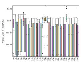
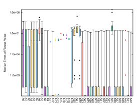
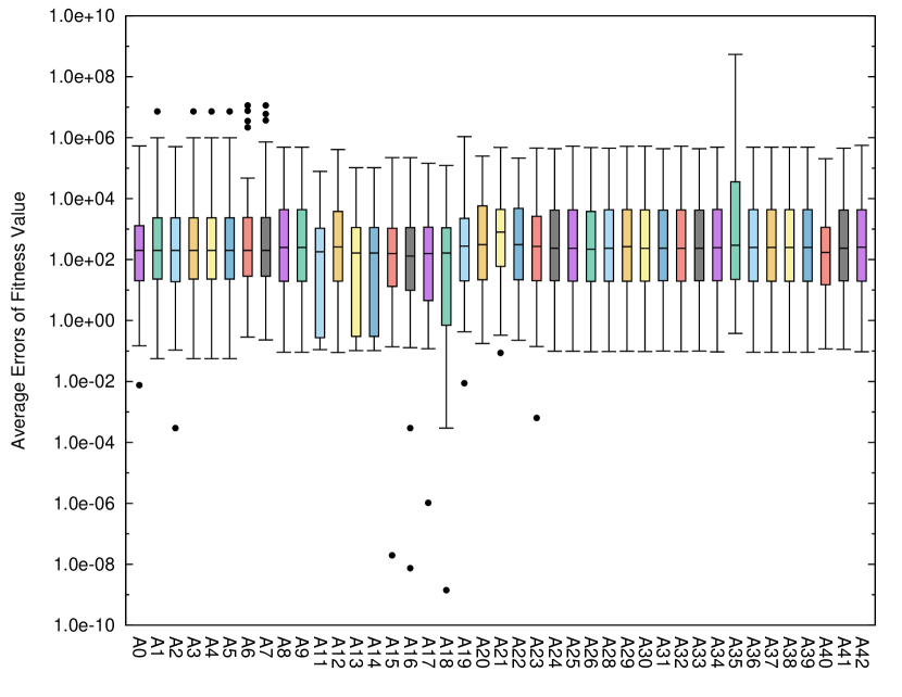
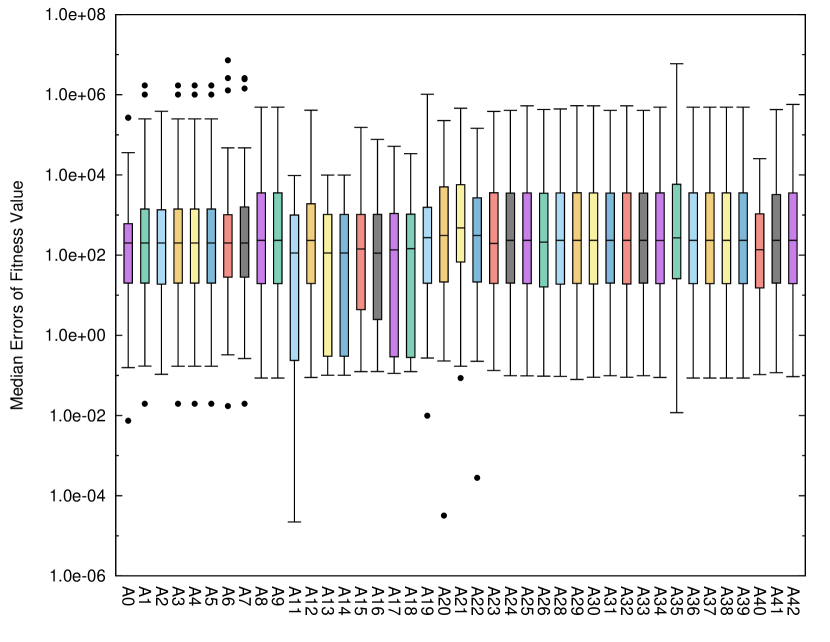
Further, the box plots for the average and median errors are shown in Figures 2(a) and 2(b) respectively. The horizontal axis represents the algorithms from the NLopt library referred by the numeric identifiers as given in Table 1, and the vertical axis represents the mean and median errors in the two cases. It may be noted that all plots indicating mean/median errors use a logarithmic scale. One can infer from the plots that in terms of average error, the choice of algorithms A6, A19, A20, A21, A22 and A35 provides better performance, whereas in case of median error, the algorithms A11, A13, A14, A15, A16, A17, A18 and A40 demonstrate superior performance.
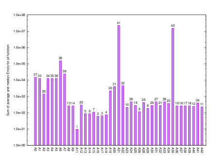
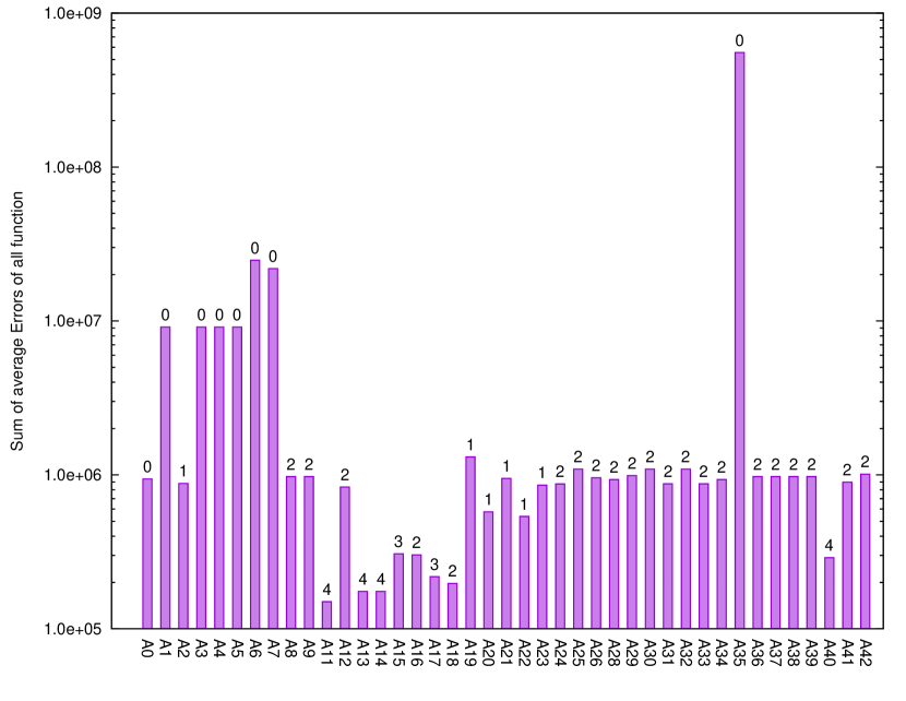
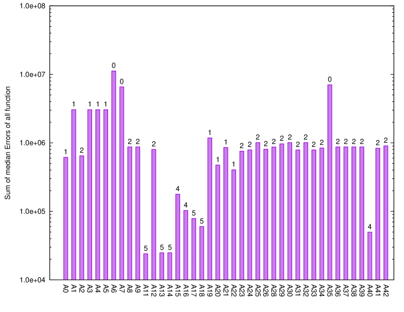
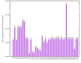
The sum of average and median errors are shown in Figures (3(a)) and (3(b)) respectively. The horizontal axis indicates the algorithm from the NLopt library, while the vertical axis shows the sum of the corresponding average and median errors. The number at the top of each bar in the graph indicates the number of times the global minima were obtained on the SOCO benchmark functions. In terms of average error, algorithms A11 and A40 are able to find the global minima for 13 and 12 functions out of the 19 benchmarks, respectively. In case of median error, algorithms A11, A15, A16, A17 and A18 are able to find global minima for 17 out of the 19 benchmark functions. None of the reference algorithms have achieved zero median error on as many functions.
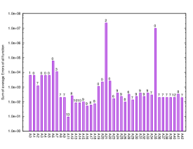
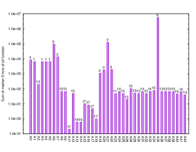
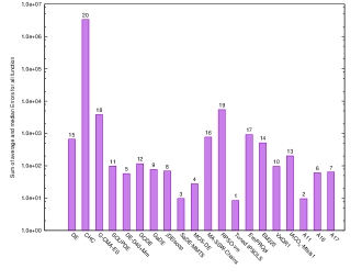
Figure 4 aims to provide a ranking of the algorithms from the NLopt library on our approach. The ranking is done on the basis of the sum of average and median errors obtained on the benchmark functions, which is indicated on the vertical axis. The bars represent the value of sum of average and median errors for the algorithms on the horizontal axis. The rank of the algorithm is indicated above the bars. From our analysis, the top three algorithms for our approach are A11 (limited memory BFGS), A16 (Truncated Newton method with restart) and A17 (Preconditioned Truncated Newton), all of which belong to the class of gradient-based methods for local search. The worst performing algorithm from our analysis is A21 (MLSL-random) which belongs to the category of gradient-based global search algorithms of the NLopt library.
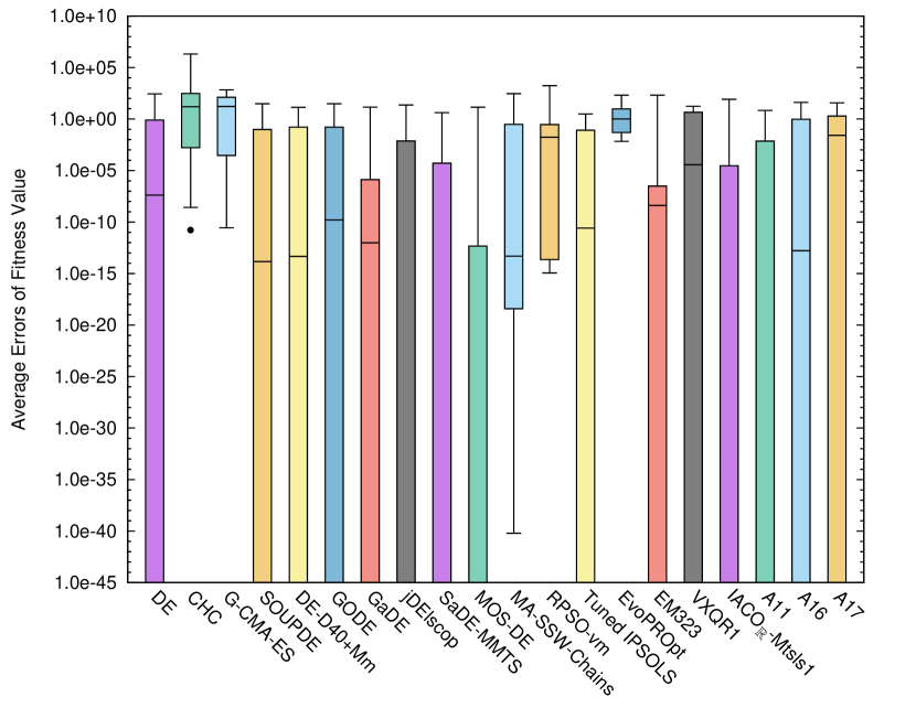
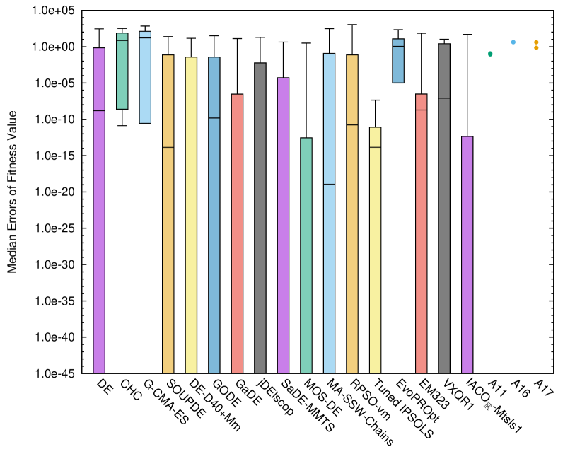
Finally, we also present a comparison of the performance of the best 3 NLopt algorithms (A11, A16 and A17) on the SOCO benchmark functions vis-à-vis reference algorithms available in literature. These include the Differential Evolution algorithm (DE) storn1997differential and its variants, the co-variance matrix adaptation evolution strategy with increasing population size (G-CMA-ES) auger2005restart , the real-coded CHC algorithm (CHC) eshelman1993chapter , Shuffle Or Update Parallel Differential Evolution (SOUPDE) weber2011shuffle , garcia2011role , Generalized Opposition-based Differential Evolution (GODE) wang2011enhanced , Generalized Adaptive Differential Evolution (GADE) yang2011scalability , jDElscop brest2011self , Self-adaptive Differential Evolution with Multi-Trajectory Search (SaDE-MMTS) zhao2011self , MOS-DE latorre2011mos , MA-SSW-Chains molina2011memetic , Restart Particle Swarm Optimization with Velocity Modulation (RPSO-VM) garcia2011restart , Tuned IPSOLS de2011incremental EVO-PROpt duarte2011path , EM323 gardeux2011em323 and VXQR neumaier2011vxqr among others.
The box plots of average and median error when comparing with -Mtsls1 are shown in Figure 5. It can be inferred that the error obtained using NLopt algorithms are much lower than the reference algorithms. A ranking of the best 3 NLopt algorithms with the reference algorithms is shown in Figure 6. The best performing algorithm was found to be the Tuned-IPSOLS, whereas CHC performs the worst.
4.2 Results on CEC 2014 benchmarks
We now present the results on the CEC 2014 benchmarks liang2013problem , where we have considered the 50-dimensional versions of the functions. The maximum number of function evaluations allowed was set to , where represents the number of dimensions in which the function is considered. The search range is , and uniform random initialization within the search space has been done. The algorithm was run times on each function; error values were defined as , where is a candidate solution and is the optimal solution. Error values lower than are approximated to 0. A summary of the benchmark functions is presented in Table 5.
| Category | S. No. | Function |
|---|---|---|
| Unimodal Functions | 1 | Rotated High Conditioned Elliptic Function |
| 2 | Rotated Bent Cigar Function | |
| 3 | Rotated Discus Function | |
| Multimodal Functions | 4 | Shifted and Rotated Rosenbrock’s Function |
| 5 | Shifted and Rotated Ackley’s Function | |
| 6 | Shifted and Rotated Weierstrass Function | |
| 7 | Shifted and Rotated Griewank’s Function | |
| 8 | Shifted Rastrigin’s Function | |
| 9 | Shifted and Rotated Rastrigin’s Function | |
| 10 | Shifted Schwefel’s Function | |
| 11 | Shifted and Rotated Schwefel’s Function | |
| 12 | Shifted and Rotated Katsuura Function | |
| 13 | Shifted and Rotated HappyCat Function | |
| 14 | Shifted and Rotated HGBat Function | |
| 15 | Shifted and Rotated Expanded Griewank’s plus Rosenbrock’s Function | |
| 16 | Shifted and Rotated Expanded Scaffer’s F6 Function | |
| Hybrid Function - 1 | 17 | Hybrid Function 1 (N=3) |
| 18 | Hybrid Function 2 (N=3) | |
| 19 | Hybrid Function 3 (N=4) | |
| 20 | Hybrid Function 4 (N=4) | |
| 21 | Hybrid Function 5 (N=5) | |
| 22 | Hybrid Function 6 (N=5) | |
| Composition Functions | 23 | Composition Function 1 (N=5) |
| 24 | Composition Function 2 (N=3) | |
| 25 | Composition Function 3 (N=3) | |
| 26 | Composition Function 4 (N=5) | |
| 27 | Composition Function 5 (N=5) | |
| 28 | Composition Function 6 (N=5) | |
| 29 | Composition Function 7 (N=3) | |
| 30 | Composition Function 8 (N=3) |
The average and median errors of the NLopt algorithms on the CEC benchmarks are shown in Figure 7. The box plots showing average error are shown in Figure 7(a), while median error is shown in Figure 7(b). It may be noted here that the plots are for the 50-dimensional versions of the functions. Further, the sum of average and median errors are shown in Figures 7(c) and 7(d) respectively.
The ranking of the algorithms on the CEC 2014 benchmarks is shown in Figure 8. One can observe that A11 (limited memory BFGS) performs the best while A35 (ISRES evolutionary constrained optimization) performs the worst.
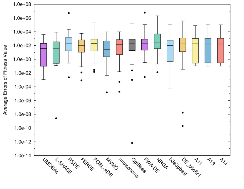
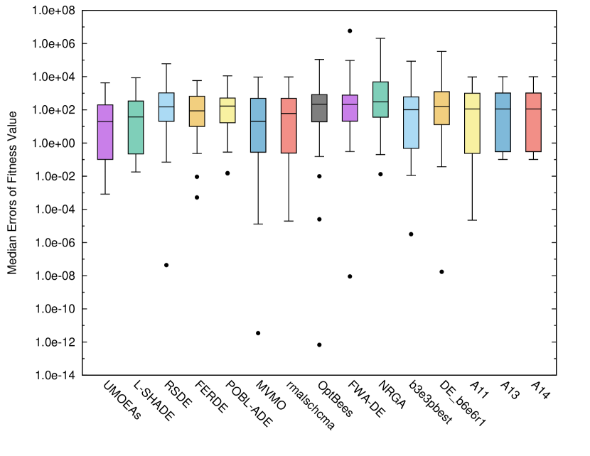
We also provide a comparison of the top 3 NLopt algorithms (A11, A13 and A14) on the CEC 2014 benchmarks with other reference algorithms. These include the United Multi-Operator Evolutionary Algorithms (UMOEA) elsayed2014testing , Success-History based Adaptive Differential Evolution using linear population size reduction (L-SHADE) tanabe2014improving , Differential Evolution with Replacement Strategy (RSDE) xu2014differential , Memetic Differential Evolution Based on Fitness Euclidean-Distance Ratio (FERDE) qu2014memetic , Partial Opposition-Based Adaptive Differential Evolution (POBL-ADE) hu2014partial , Mean-Variance Mapping Optimization (MVMO) erlich2014evaluating , rmalschcma molina2014influence , Opt Bees maia2014real , Fireworks Algorithm with Differential Mutation (FWA-DE) yu2014fireworks , Non-uniform Real-coded Genetic Algorithm (NRGA) yashesh2014non , b3e3pbest bujok2014differential and DE_b6e6rl polakova2014controlled .
The box plots for average and median errors are shown in Figure 9, specifically average error in Figure (9(a)) and median error in Figure (9(b)) respectively. The range of average errors of the reference algorithms are relatively lower than the top 3 NLopt algorithms except on UMOEA, and also median error except MVMO and rmalschcma.
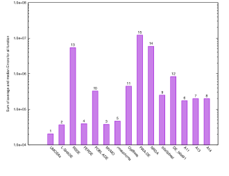
A relative ranking of these algorithms is shown in Figure 10. One can observe that the best performing algorithm is UMOEA, while the worst performing algorithm is FWA-DE.
4.3 Comparison of Hybrid approach with standalone algorithms used for Local Search
We also provide a comparison of the standalone performance of the algorithms in Table 6. The comparison is provided in terms of Wilcoxon Signed-Rank test wilcoxon1945individual , which is a measure of the extent of statistical deviations in the results obtained using a particular approach. A p-value less than indicates that the results of our approach have a significant statistical difference with the results obtained using the algorithms being compared, whereas p-values greater than indicate non-significant statistical difference. The columns and denote the sum of signed ranks. The column indicates the number of instances for which there is a difference in the result between two algorithms.
It can be observed from Table 6 that on the SOCO benchmark functions, the NLopt algorithms give significant statistical difference on all but one (A34) in terms of average error, and on all but two (A6 and A7) in terms of median error. On the CEC 2014 benchmarks, there is significant statistical difference on all but 8 and 3 out of 42 algorithms in terms of average and median error respectively.
| SOCO | CEC2014 | |||||||||||||||
| Average | Median | Average | Median | |||||||||||||
| Wp | Wn | n | p | Wp | Wn | n | p | Wp | Wn | n | p | Wp | Wn | n | p | |
| A0 | 7 | 183 | 19 | 3.98E-04 | 0 | 78 | 12 | 4.88E-04 | 26 | 250 | 23 | 6.58E-04 | 0 | 190 | 19 | 1.32E-04 |
| A1 | 4 | 186 | 19 | 2.50E-04 | 0 | 91 | 13 | 2.44E-04 | 32 | 268 | 24 | 7.48E-04 | 0 | 153 | 17 | 2.93E-04 |
| A2 | 0 | 190 | 19 | 1.32E-04 | 0 | 190 | 19 | 1.32E-04 | 26 | 274 | 24 | 3.96E-04 | 0 | 231 | 21 | 5.96E-05 |
| A3 | 3 | 187 | 19 | 2.14E-04 | 0 | 91 | 13 | 2.44E-04 | 32 | 268 | 24 | 7.48E-04 | 0 | 153 | 17 | 2.93E-04 |
| A4 | 3 | 187 | 19 | 2.14E-04 | 0 | 91 | 13 | 2.44E-04 | 32 | 268 | 24 | 7.48E-04 | 0 | 153 | 17 | 2.93E-04 |
| A5 | 3 | 187 | 19 | 2.14E-04 | 0 | 91 | 13 | 2.44E-04 | 32 | 268 | 24 | 7.48E-04 | 0 | 153 | 17 | 2.93E-04 |
| A6 | 0 | 190 | 19 | 1.32E-04 | 0 | 0 | 0 | 1.00E+00 | 33 | 243 | 23 | 1.41E-03 | 0 | 105 | 14 | 1.22E-04 |
| A7 | 2 | 134 | 16 | 6.43E-04 | 0 | 0 | 0 | 1.00E+00 | 33 | 243 | 23 | 1.41E-03 | 0 | 91 | 13 | 2.44E-04 |
| A8 | 0 | 190 | 19 | 1.32E-04 | 0 | 190 | 19 | 1.32E-04 | 61 | 404 | 30 | 4.20E-04 | 62 | 403 | 30 | 4.53E-04 |
| A9 | 0 | 190 | 19 | 1.32E-04 | 0 | 190 | 19 | 1.32E-04 | 61 | 404 | 30 | 4.20E-04 | 62 | 403 | 30 | 4.53E-04 |
| A11 | 1 | 135 | 16 | 5.31E-04 | 0 | 91 | 13 | 2.44E-04 | 109 | 216 | 25 | 1.50E-01 | 68 | 208 | 23 | 3.33E-02 |
| A12 | 1 | 152 | 17 | 3.52E-04 | 1 | 135 | 16 | 5.31E-04 | 71 | 307 | 27 | 4.58E-03 | 72 | 306 | 27 | 4.94E-03 |
| A13 | 0 | 153 | 17 | 2.93E-04 | 2 | 134 | 16 | 6.43E-04 | 109 | 242 | 26 | 9.12E-02 | 29 | 247 | 23 | 9.16E-04 |
| A14 | 0 | 153 | 17 | 2.93E-04 | 2 | 134 | 16 | 6.43E-04 | 109 | 242 | 26 | 9.12E-02 | 29 | 247 | 23 | 9.16E-04 |
| A15 | 0 | 136 | 16 | 4.38E-04 | 0 | 120 | 15 | 6.10E-05 | 93 | 313 | 28 | 1.23E-02 | 32 | 374 | 28 | 9.86E-05 |
| A16 | 0 | 136 | 16 | 4.38E-04 | 0 | 120 | 15 | 6.10E-05 | 91 | 315 | 28 | 1.08E-02 | 34 | 344 | 27 | 1.96E-04 |
| A17 | 3 | 150 | 17 | 5.03E-04 | 0 | 120 | 15 | 6.10E-05 | 93 | 285 | 27 | 2.11E-02 | 36 | 315 | 26 | 3.96E-04 |
| A18 | 1 | 152 | 17 | 3.52E-04 | 0 | 105 | 14 | 1.22E-04 | 92 | 286 | 27 | 1.98E-02 | 29 | 271 | 24 | 5.46E-04 |
| A19 | 15 | 175 | 19 | 1.28E-03 | 16 | 174 | 19 | 1.48E-03 | 147 | 288 | 29 | 1.27E-01 | 98 | 253 | 26 | 5.05E-02 |
| A20 | 17 | 173 | 19 | 1.70E-03 | 7 | 183 | 19 | 3.98E-04 | 71 | 254 | 25 | 1.38E-02 | 62 | 238 | 24 | 1.19E-02 |
| A21 | 0 | 153 | 17 | 2.93E-04 | 0 | 153 | 17 | 2.92E-04 | 53 | 325 | 27 | 1.08E-03 | 31 | 320 | 26 | 2.42E-04 |
| A22 | 18 | 172 | 19 | 1.94E-03 | 13 | 177 | 19 | 9.67E-04 | 95 | 230 | 25 | 6.73E-02 | 78 | 247 | 25 | 2.30E-02 |
| A23 | 0 | 153 | 17 | 2.93E-04 | 2 | 151 | 17 | 4.21E-04 | 66 | 340 | 28 | 1.81E-03 | 57 | 294 | 26 | 2.62E-03 |
| A24 | 0 | 153 | 17 | 2.93E-04 | 0 | 153 | 17 | 2.93E-04 | 52 | 354 | 28 | 5.85E-04 | 44 | 307 | 26 | 8.38E-04 |
| A25 | 0 | 190 | 19 | 1.32E-04 | 0 | 190 | 19 | 1.32E-04 | 99 | 336 | 29 | 1.04E-02 | 99 | 336 | 29 | 1.04E-02 |
| A26 | 0 | 190 | 19 | 1.32E-04 | 0 | 190 | 19 | 1.32E-04 | 240 | 195 | 29 | 6.27E-01 | 229 | 236 | 30 | 9.34E-01 |
| A28 | 0 | 190 | 19 | 1.32E-04 | 0 | 190 | 19 | 1.32E-04 | 83 | 382 | 30 | 2.11E-03 | 86 | 379 | 30 | 2.58E-03 |
| A29 | 0 | 190 | 19 | 1.32E-04 | 0 | 190 | 19 | 1.32E-04 | 56 | 409 | 30 | 2.83E-04 | 88 | 377 | 30 | 2.96E-03 |
| A30 | 0 | 190 | 19 | 1.32E-04 | 0 | 190 | 19 | 1.32E-04 | 99 | 336 | 29 | 1.04E-02 | 99 | 336 | 29 | 1.04E-02 |
| A31 | 0 | 153 | 17 | 2.93E-04 | 0 | 153 | 17 | 2.93E-04 | 38 | 340 | 27 | 2.86E-04 | 33 | 318 | 26 | 2.96E-04 |
| A32 | 0 | 190 | 19 | 1.32E-04 | 0 | 190 | 19 | 1.32E-04 | 99 | 336 | 29 | 1.04E-02 | 99 | 336 | 29 | 1.04E-02 |
| A33 | 0 | 153 | 17 | 2.93E-04 | 0 | 153 | 17 | 2.93E-04 | 38 | 340 | 27 | 2.86E-04 | 33 | 318 | 26 | 2.96E-04 |
| A34 | 38 | 115 | 17 | 6.84E-02 | 0 | 153 | 17 | 2.93E-04 | 253 | 182 | 29 | 4.43E-01 | 229 | 149 | 27 | 3.37E-01 |
| A35 | 0 | 190 | 19 | 1.32E-04 | 9 | 181 | 19 | 5.39E-04 | 2 | 433 | 29 | 3.17E-06 | 0 | 435 | 29 | 2.56E-06 |
| A36 | 0 | 190 | 19 | 1.32E-04 | 0 | 190 | 19 | 1.32E-04 | 61 | 404 | 30 | 4.20E-04 | 62 | 403 | 30 | 4.53E-04 |
| A37 | 0 | 190 | 19 | 1.32E-04 | 0 | 190 | 19 | 1.32E-04 | 61 | 404 | 30 | 4.20E-04 | 62 | 403 | 30 | 4.53E-04 |
| A38 | 0 | 190 | 19 | 1.32E-04 | 0 | 190 | 19 | 1.32E-04 | 61 | 404 | 30 | 4.20E-04 | 62 | 403 | 30 | 4.53E-04 |
| A39 | 0 | 190 | 19 | 1.32E-04 | 0 | 190 | 19 | 1.32E-04 | 61 | 404 | 30 | 4.20E-04 | 62 | 403 | 30 | 4.53E-04 |
| A40 | 0 | 136 | 16 | 4.38E-04 | 0 | 136 | 16 | 4.38E-04 | 99 | 226 | 25 | 8.75E-02 | 62 | 214 | 23 | 2.08E-02 |
| A41 | 0 | 153 | 17 | 2.93E-04 | 0 | 153 | 17 | 2.93E-04 | 71 | 335 | 28 | 2.65E-03 | 38 | 313 | 26 | 4.79E-04 |
| A42 | 0 | 190 | 19 | 1.32E-04 | 0 | 190 | 19 | 1.32E-04 | 37 | 428 | 30 | 5.79E-05 | 37 | 428 | 30 | 5.79E-05 |
5 Conclusions
This paper presented an exhaustive analysis of using optimization algorithms from the NLopt library in combination with the Mtsls1 algorithm within the -Mtsls1 framework for continuous global optimization. The results on SOCO and CEC 2014 benchmark functions present a ready reference on the performance of these approaches and would be of help to a researcher in deciding on a choice among these algorithms. The nature of functions on which these algorithms perform better can also be inferred from the results. A relative ranking of these approaches has also been provided based on the total error obtained in using them, which would provide a measure of the versatility of the algorithms.
The results of our analysis have been summarized in Table 7. On both the benchmark function sets, the hybrid -Mtsls1 with gradient-based local search performs better (A11, A16, A17 for SOCO and A11, A13, A14 for CEC). The best results are obtained using hybridization with BFGS on both benchmarks. On SOCO benchmarks, the hybrid approach outperforms the original -Mtsls1, as it has been able to achieve zero median error on 17 out of 19 functions, which has not been achieved by any other algorithm considered. We believe that the analysis presented in this paper would be of use to the research community at large.
| Function | Ranking | NLopt | State-of-Art |
|---|---|---|---|
| SOCO | Best | A11 | Tuned IPSOLS |
| Worst | A21 | CHC | |
| CEC 2014 | Best | A11 | UMOEA |
| Worst | A35 | FWA-DE | |
| A11: Limited Memory BFGS | |||
| A21: Multi-Level Single Linkage, random | |||
| A35: ISRES Evolutionary Constrained Optimization | |||
| Tuned IPSOLS: Incremental Particle Swarm for Large Scale Optimization | |||
| UMOEA: united Multi Operator Evolutionary Algorithms | |||
| FWA-DE: FireWorks Algorithm with Differential Evolution | |||
References
- [1] Anne Auger and Nikolaus Hansen. A restart CMA evolution strategy with increasing population size. In Evolutionary Computation, 2005. The 2005 IEEE Congress on, volume 2, pages 1769–1776. IEEE, 2005.
- [2] Ernesto G Birgin and José Mario Martínez. Improving ultimate convergence of an augmented lagrangian method. Optimization Methods and Software, 23(2):177–195, 2008.
- [3] Richard P Brent. Algorithms for minimization without derivatives. Courier Dover Publications, 1973.
- [4] Janez Brest and Mirjam Sepesy Maučec. Self-adaptive differential evolution algorithm using population size reduction and three strategies. Soft Computing, 15(11):2157–2174, 2011.
- [5] Petr Bujok, Josef Tvrdik, and Radka Polakova. Differential evolution with rotation-invariant mutation and competing-strategies adaptation. In Evolutionary Computation (CEC), 2014 IEEE Congress on, pages 2253–2258. IEEE, 2014.
- [6] Q Chen, B Liu, Q Zhang, JJ Liang, PN Suganthan, and BY Qu. Problem definition and evaluation criteria for CEC 2015 special session and competition on bound constrained single-objective computationally expensive numerical optimization.
- [7] Andrew R Conn, Nicholas IM Gould, and Philippe Toint. A globally convergent augmented lagrangian algorithm for optimization with general constraints and simple bounds. SIAM Journal on Numerical Analysis, 28(2):545–572, 1991.
- [8] Swagatam Das, Sayan Maity, Bo-Yang Qu, and Ponnuthurai Nagaratnam Suganthan. Real-parameter evolutionary multimodal optimization—a survey of the state-of-the-art. Swarm and Evolutionary Computation, 1(2):71–88, 2011.
- [9] Swagatam Das and Ponnuthurai Nagaratnam Suganthan. Differential Evolution: a survey of the state-of-the-art. Evolutionary Computation, IEEE Transactions on, 15(1):4–31, 2011.
- [10] Marco A Montes de Oca, Doğan Aydın, and Thomas Stützle. An incremental particle swarm for large-scale continuous optimization problems: an example of tuning-in-the-loop (re) design of optimization algorithms. Soft Computing, 15(11):2233–2255, 2011.
- [11] Ron S Dembo and Trond Steihaug. Truncated newton algorithms for large-scale unconstrained optimization. Mathematical Programming, 26(2):190–212, 1983.
- [12] Abraham Duarte, Rafael Martí, and Francisco Gortazar. Path relinking for large-scale global optimization. Soft Computing, 15(11):2257–2273, 2011.
- [13] Saber M Elsayed, Ruhul A Sarker, Daryl L Essam, and Noha M Hamza. Testing united multi-operator evolutionary algorithms on the CEC 2014 real-parameter numerical optimization. In Evolutionary Computation (CEC), 2014 IEEE Congress on, pages 1650–1657. IEEE, 2014.
- [14] Istvan Erlich, Jose L Rueda, Sebastian Wildenhues, and Fekadu Shewarega. Evaluating the mean-variance mapping optimization on the IEEE-CEC 2014 test suite. In Evolutionary Computation (CEC), 2014 IEEE Congress on, pages 1625–1632. IEEE, 2014.
- [15] Larry J Eshelman. chapter real-coded genetic algorithms and interval-schemata. Foundations of genetic algorithms, 2:187–202, 1993.
- [16] Daniel E Finkel. DIRECT optimization algorithm user guide. Center for Research in Scientific Computation, North Carolina State University, 2, 2003.
- [17] Joerg M Gablonsky and C Tim Kelley. A locally-biased form of the DIRECT algorithm. Journal of Global Optimization, 21(1):27–37, 2001.
- [18] Carlos García-Martínez, Francisco J Rodríguez, and Manuel Lozano. Role differentiation and malleable mating for differential evolution: an analysis on large-scale optimisation. Soft Computing, 15(11):2109–2126, 2011.
- [19] José García-Nieto and Enrique Alba. Restart particle swarm optimization with velocity modulation: a scalability test. Soft Computing, 15(11):2221–2232, 2011.
- [20] Vincent Gardeux, Rachid Chelouah, Patrick Siarry, and Fred Glover. EM323: a line search based algorithm for solving high-dimensional continuous non-linear optimization problems. Soft Computing, 15(11):2275–2285, 2011.
- [21] S Gudmundsson. Parallel Global Optimization. 1998.
- [22] F Herrera, M Lozano, and D Molina. Test suite for the special issue of soft computing on scalability of evolutionary algorithms and other metaheuristics for large scale continuous optimization problems. URL: http://sci2s.ugr.es/eamhco/updated-functions1-19.pdf, Published 2010.
- [23] Zhongyi Hu, Yukun Bao, and Tao Xiong. Partial opposition-based adaptive differential evolution algorithms: Evaluation on the CEC 2014 benchmark set for real-parameter optimization. In Evolutionary Computation (CEC), 2014 IEEE Congress on, pages 2259–2265. IEEE, 2014.
- [24] Steven G Johnson. The NLopt nonlinear-optimization package, 2010.
- [25] Donald R Jones, Cary D Perttunen, and Bruce E Stuckman. Lipschitzian optimization without the Lipschitz constant. Journal of Optimization Theory and Applications, 79(1):157–181, 1993.
- [26] P Kaelo and MM Ali. Some variants of the controlled random search algorithm for global optimization. Journal of optimization theory and applications, 130(2):253–264, 2006.
- [27] AHG Rinnooy Kan and GT Timmer. Stochastic global optimization methods part i: Clustering methods. Mathematical programming, 39(1):27–56, 1987.
- [28] Dieter Kraft. A software package for sequential quadratic programming. DFVLR Obersfaffeuhofen, Germany, 1988.
- [29] Dieter Kraft. Algorithm 733: TOMP–fortran modules for optimal control calculations. ACM Transactions on Mathematical Software (TOMS), 20(3):262–281, 1994.
- [30] Jeffrey C Lagarias, James A Reeds, Margaret H Wright, and Paul E Wright. Convergence properties of the Nelder–Mead simplex method in low dimensions. SIAM Journal on optimization, 9(1):112–147, 1998.
- [31] Antonio LaTorre, Santiago Muelas, and José-María Peña. A MOS-based dynamic memetic differential evolution algorithm for continuous optimization: a scalability test. Soft Computing, 15(11):2187–2199, 2011.
- [32] Dong-Hui Li and Masao Fukushima. A modified BFGS method and its global convergence in nonconvex minimization. Journal of Computational and Applied Mathematics, 129(1):15–35, 2001.
- [33] JJ Liang, BY Qu, and PN Suganthan. Problem definitions and evaluation criteria for the CEC 2014 special session and competition on single objective real-parameter numerical optimization. Computational Intelligence Laboratory, Zhengzhou University, Zhengzhou China and Technical Report, Nanyang Technological University, Singapore, 2013.
- [34] Tianjun Liao, Marco A Montes de Oca, Dogan Aydin, Thomas Stützle, and Marco Dorigo. An incremental ant colony algorithm with local search for continuous optimization. In Proceedings of the 13th annual conference on Genetic and evolutionary computation, pages 125–132. ACM, 2011.
- [35] Dong C Liu and Jorge Nocedal. On the limited memory BFGS method for large scale optimization. Mathematical programming, 45(1-3):503–528, 1989.
- [36] Manuel Lozano, Daniel Molina, and Francisco Herrera. Editorial scalability of evolutionary algorithms and other metaheuristics for large-scale continuous optimization problems. Soft Computing, 15(11):2085–2087, 2011.
- [37] Kaj Madsen, Serguei Zertchaninov, and Antanas Zilinskas. Global optimization using branch-and-bound. Submitted to Global Optimization, 1998.
- [38] Renato Dourado Maia, Leandro Nunes de Castro, and Walmir Matos Caminhas. Real-parameter optimization with OptBees. In Evolutionary Computation (CEC), 2014 IEEE Congress on, pages 2649–2655. IEEE, 2014.
- [39] Daniel Molina, Benjamin Lacroix, and Francisco Herrera. Influence of regions on the memetic algorithm for the CEC 2014 special session on real-parameter single objective optimisation. In Evolutionary Computation (CEC), 2014 IEEE Congress on, pages 1633–1640. IEEE, 2014.
- [40] Daniel Molina, Manuel Lozano, Ana M Sánchez, and Francisco Herrera. Memetic algorithms based on local search chains for large scale continuous optimisation problems: MA-SSW-chains. Soft Computing, 15(11):2201–2220, 2011.
- [41] John A Nelder and Roger Mead. A simplex method for function minimization. The computer journal, 7(4):308–313, 1965.
- [42] Arnold Neumaier, Hannes Fendl, Harald Schilly, and Thomas Leitner. VXQR: Derivative-free unconstrained optimization based on QR factorizations. Soft Computing, 15(11):2287–2298, 2011.
- [43] Radka Polakova, Josef Tvrdik, and Petr Bujok. Controlled restart in differential evolution applied to CEC 2014 benchmark functions. In Evolutionary Computation (CEC), 2014 IEEE Congress on, pages 2230–2236. IEEE, 2014.
- [44] Michael JD Powell. A direct search optimization method that models the objective and constraint functions by linear interpolation. In Advances in optimization and numerical analysis, pages 51–67. Springer, 1994.
- [45] Michael JD Powell. The NEWUOA software for unconstrained optimization without derivatives. In Large-scale nonlinear optimization, pages 255–297. Springer, 2006.
- [46] Michael JD Powell. Developments of NEWUOA for unconstrained minimization without derivatives. Dept. Appl. Math. Theoretical Phys., Univ. Cambridge, Cambridge, UK, Tech. Rep. DAMTP, 2007.
- [47] Michael JD Powell. Developments of NEWUOA for minimization without derivatives. IMA journal of numerical analysis, 28(4):649–664, 2008.
- [48] Michael JD Powell. The BOBYQA algorithm for bound constrained optimization without derivatives. Cambridge NA Report NA2009/06, University of Cambridge, Cambridge, 2009.
- [49] BY Qu, JJ Liang, JM Xiao, and ZG Shang. Memetic differential evolution based on fitness euclidean-distance ratio. In Evolutionary Computation (CEC), 2014 IEEE Congress on, pages 2266–2273. IEEE, 2014.
- [50] Luis Miguel Rios and Nikolaos V Sahinidis. Derivative-free optimization: a review of algorithms and comparison of software implementations. Journal of Global Optimization, 56(3):1247–1293, 2013.
- [51] Thomas Harvey Rowan. Functional stability analysis of numerical algorithms. 1990.
- [52] Thomas Philip Runarsson and Xin Yao. Search biases in constrained evolutionary optimization. Systems, Man, and Cybernetics, Part C: Applications and Reviews, IEEE Transactions on, 35(2):233–243, 2005.
- [53] Ralf Salomon. Evolutionary algorithms and gradient search: similarities and differences. Evolutionary Computation, IEEE Transactions on, 2(2):45–55, 1998.
- [54] C Hd S Santos, Marcos Sergio Goncalves, and Hugo Enrique Hernandez-Figueroa. Designing novel photonic devices by bio-inspired computing. Photonics Technology Letters, IEEE, 22(15):1177–1179, 2010.
- [55] JA Snyman and LP Fatti. A multi-start global minimization algorithm with dynamic search trajectories. Journal of Optimization Theory and Applications, 54(1):121–141, 1987.
- [56] Rainer Storn and Kenneth Price. Differential evolution–a simple and efficient heuristic for global optimization over continuous spaces. Journal of global optimization, 11(4):341–359, 1997.
- [57] Krister Svanberg. A class of globally convergent optimization methods based on conservative convex separable approximations. SIAM journal on optimization, 12(2):555–573, 2002.
- [58] Ryoji Tanabe and Alex S Fukunaga. Improving the search performance of SHADE using linear population size reduction. In Evolutionary Computation (CEC), 2014 IEEE Congress on, pages 1658–1665. IEEE, 2014.
- [59] Ke Tang, Xın Yáo, Ponnuthurai Nagaratnam Suganthan, Cara MacNish, Ying-Ping Chen, Chih-Ming Chen, and Zhenyu Yang. Benchmark functions for the cec’2008 special session and competition on large scale global optimization. Nature Inspired Computation and Applications Laboratory, USTC, China, 2007.
- [60] Lin-Yu Tseng and Chun Chen. Multiple trajectory search for large scale global optimization. In Evolutionary Computation, 2008. CEC 2008.(IEEE World Congress on Computational Intelligence). IEEE Congress on, pages 3052–3059. IEEE, 2008.
- [61] Lin-Yu Tseng and Chun Chen. Multiple trajectory search for unconstrained/constrained multi-objective optimization. In Evolutionary Computation, 2009. CEC’09. IEEE Congress on, pages 1951–1958. IEEE, 2009.
- [62] Jan Vlček and Ladislav Lukšan. Shifted limited-memory variable metric methods for large-scale unconstrained optimization. Journal of Computational and Applied Mathematics, 186(2):365–390, 2006.
- [63] Zhong Wan, Kok Lay Teo, XianLong Shen, and ChaoMing Hu. New BFGS method for unconstrained optimization problem based on modified Armijo line search. Optimization, 63(2):285–304, 2014.
- [64] Hui Wang, Zhijian Wu, and Shahryar Rahnamayan. Enhanced opposition-based differential evolution for solving high-dimensional continuous optimization problems. Soft Computing, 15(11):2127–2140, 2011.
- [65] Matthieu Weber, Ferrante Neri, and Ville Tirronen. Shuffle or update parallel differential evolution for large-scale optimization. Soft Computing, 15(11):2089–2107, 2011.
- [66] Zengxin Wei, Gaohang Yu, Gonglin Yuan, and Zhigang Lian. The superlinear convergence of a modified BFGS-type method for unconstrained optimization. Computational optimization and applications, 29(3):315–332, 2004.
- [67] Frank Wilcoxon. Individual comparisons by ranking methods. Biometrics bulletin, pages 80–83, 1945.
- [68] SJ Wright and J Nocedal. Numerical optimization, volume 2. Springer New York, 1999.
- [69] Changjian Xu, Han Huang, and Shujin Ye. A differential evolution with replacement strategy for real-parameter numerical optimization. In Evolutionary Computation (CEC), 2014 IEEE Congress on, pages 1617–1624. IEEE, 2014.
- [70] Zhenyu Yang, Ke Tang, and Xin Yao. Scalability of generalized adaptive differential evolution for large-scale continuous optimization. Soft Computing, 15(11):2141–2155, 2011.
- [71] Dhebar Yashesh, Kalyanmoy Deb, and Sunith Bandaru. Non-uniform mapping in real-coded genetic algorithms. In Evolutionary Computation (CEC), 2014 IEEE Congress on, pages 2237–2244. IEEE, 2014.
- [72] Chao Yu, Lingchen Kelley, Shaoqiu Zheng, and Ying Tan. Fireworks algorithm with differential mutation for solving the CEC 2014 competition problems. In Evolutionary Computation (CEC), 2014 IEEE Congress on, pages 3238–3245. IEEE, 2014.
- [73] Serguei Zertchaninov and Kaj Madsen. A C++ Programme for Global Optimization. IMM, Department of Mathematical Modelling, Technical Universityof Denmark, 1998.
- [74] Shi-Zheng Zhao, Ponnuthurai Nagaratnam Suganthan, and Swagatam Das. Self-adaptive differential evolution with multi-trajectory search for large-scale optimization. Soft Computing, 15(11):2175–2185, 2011.
- [75] Aimin Zhou, Bo-Yang Qu, Hui Li, Shi-Zheng Zhao, Ponnuthurai Nagaratnam Suganthan, and Qingfu Zhang. Multiobjective evolutionary algorithms: A survey of the state of the art. Swarm and Evolutionary Computation, 1(1):32–49, 2011.