Solving Local Linear Systems with Boundary Conditions Using Heat Kernel Pagerank

Abstract

We present an efficient algorithm for solving local linear systems with a boundary condition using the Green’s function of a connected induced subgraph related to the system. We introduce the method of using the Dirichlet heat kernel pagerank vector to approximate local solutions to linear systems in the graph Laplacian satisfying given boundary conditions over a particular subset of vertices. With an efficient algorithm for approximating Dirichlet heat kernel pagerank, our local linear solver algorithm computes an approximate local solution with multiplicative and additive error $\epsilon$ by performing $O(\epsilon^{-5}s^{3}\log(s^{3}\epsilon^{-1})\log n)$ random walk steps, where $n$ is the number of vertices in the full graph and $s$ is the size of the local system on the induced subgraph.

1 Introduction

There are a number of linear systems which model flow over vertices of a graph with a given boundary condition. A classical example is the case of an electrical network. Flow can be captured by measuring electric current between points in the network, and the amount that is injected and removed from the system. Here, the points at which voltage potential is measured can be represented by vertices in a graph, and edges are associated to the ease with which current passes between two points. The injection and extraction points can be viewed as the boundary of the system, and the relationship of the flow and voltage can be evaluated by solving a system of linear equations over the measurement points.

Another example is a decision-making process among a network of agents. Each agent decides on a value, but may be influenced by the decision of other agents in the network. Over time, the goal is to reach consensus among all the agents, in which each agrees on a common value. Agents are represented by vertices, and each vertex has an associated value. The amount of influence an agent has on a fellow agent is modeled by a weighted edge between the two representative vertices, and the communication dynamics can be modeled by a linear system. In this case, some special agents which make their own decisions can be viewed as the boundary.

In both these cases, the linear systems are equations formulated in the graph Laplacian. Spectral properties of the Laplacian are closely related to reachability and the rate of diffusion across vertices in a graph [4]. Laplacian systems have been used to concisely characterize qualities such as edge resistance and the influence of communication on edges [23]. There is a substantial body of work on efficient and nearly-linear time solvers for Laplacian linear systems ([10, 24, 26, 15, 16, 17, 13, 14, 2, 21, 22, 8], see also [27]).

The focus of this paper is a localized version of a Laplacian linear solver. In a large network, possibly of hundreds of millions of vertices, the algorithms we are dealing with and the solutions we are seeking are usually of finite support. Here, by finite we mean the support size depends only on the requested output and is independent of the full size of the network. Sometimes we allow sizes up to a factor of $\log(n)$, where $n$ is the size of the network.

The setup is a graph and a boundary condition given by a vector with specified limited support over the vertices. In the local setting, rather than computing the full solution we compute the solution over a fraction of the graph and de facto ignore the vertices with solution values below the multiplicative/additive error bound. In essence we avoid computing the entire solution by focusing computation on the subset itself. In this way, computation depends on the size of the subset, rather than the size of the full graph. We distinguish the two cases as “global” and “local” linear solvers, respectively. We remark that in the case the solution is not “local,” for example, if all values are below the error bound, our alogrithm will return the zero vector – a valid approximate solution according to our definition of approximation.

In this paper, we show how local Laplacian linear systems with a boundary condition can be solved and efficiently approximated by using Dirichlet heat kernel pagerank, a diffusion process over an induced subgraph. We will illustrate the connection between the Dirichlet heat kernel pagerank vector and the Green’s function, or the inverse of a submatrix of the Laplacian determined by the subset. We also demonstrate the method of approximation using random walks. Our algorithm approximates the solution to the system restricted to the subset $S$ by performing $O\left(\gamma^{-2}\epsilon^{-3}s^{3}\log^{2}(s^{3}\gamma^{-1})\log n\right)$ random walk steps, where $\gamma$ is the error bound for the solver and $\epsilon$ is the error bound for Dirichlet heat kernel pagerank approximation, and $s$ denotes the size of $S$. We assume that performing a random walk step and drawing from a distribution with finite support require constant time. With this, our algorithm runs in time $O\left(\gamma^{-2}\epsilon^{-3}\log^{4}(n)\log^{2}(\gamma^{-1}\log^{3}(n))\right)$ when the support size of the solution is $O(\log n)$. Note that in our computation, we do not intend to compute or approximate the matrix form of the inverse of the Laplacian. We intend to compute an approximate local solution which is optimal subject to the (relaxed) definition of approximation.

1.1 A Summary of the Main Results

We give an algorithm called Local Linear Solverfor approximating a local solution of a Laplacian linear system with a boundary condition. The algorithm uses the connection between the inverse of the restricted Laplacian and the Dirichlet heat kernel of the graph for approximating the local solution with a sampling of Dirichlet heat kernel pagerank vectors (heat kernel pagerank restricted to a subset $S$). It is shown in Theorem 4.3 that the output of Local Linear Solver approximates the exact local solution $x_{S}$ with absolute error $O(\gamma||b||+||x_{S}||)$ for boundary vector $b$ with probability at least $1-\gamma$.

We present an efficient algorithm for approximating Dirichlet heat kernel pagerank vectors, ApproxDirHKPR. The algorithm is an extension of the algorithm in [7]. The definition of $\epsilon$-approximate vectors is given in Section 5. We note that this notion of approximation is weaker than the classical notions of total variation distance among others. Nevertheless, this “relaxed” notion of approximation is used in analyzing PageRank algorithms (see [3], for example) for massive networks.

The full algorithm for approximating a local linear solution, GreensSolver, is presented in Section 6. The algorithm is an invocation of Local Linear Solver with the ApproxDirHKPR called as a subroutine. The full agorithm requires $O\left(\gamma^{-2}\epsilon^{-3}s^{3}\log^{2}(s^{3}\gamma^{-1})\log n\right)$ random walk steps by using the algorithm ApproxDirHKPR with a slight modification. Our algorithm achieves sublinear time after preprocessing which depends on the size of the support of the boundary condition. The error is similar to the error of ApproxDirHKPR.

It is worth pointing out a number of ways our methods can be generalized. First, we focus on unweighted graphs, though extending our results to graphs with edge weights follows easily with a weighted version of the Laplacian. Second, we require the induced subgraph on the subset $S$ be connected. However, if the induced subgraph is not connected the results can be applied to components separately, so our requirement on connectivity can be relaxed. Finally, we restrict our discussion to linear systems in the graph Laplacian. However, by using a linear-time transformation due to [11] for converting a symmetric, diagonally dominant linear system to a Laplacian linear system, our results apply to a larger class of linear systems.

1.2 Organization

In Section 2, we give definitions and basic facts for graph Laplacian and heat kernel. In Section 3 the problem is introduced in detail and provides the setting for the local solver. The algorithm, Local Linear Solver, is presented in Section 4. After this, we extend the solver to the full approximation algorithm using approximate Dirichlet heat kernel pagerank. In Section 5, we give the definition of local approximation and analyze the Dirichlet heat kernel pagerank approximation algorithm. In Section 6, the full algorithm for computing an approximate local solution to a Laplacian linear system with a boundary condition, GreensSolver, is given. Finally in Section 7 we illustrate the correctness of the algorithm with an example network and specified boundary condition. The example demonstrates visually what a local solution is and how GreensSolver successfully approximates the solution within the prescribed error bounds when the solution is sufficiently local.

2 Basic Definitions and Facts

Let $G$ be a simple graph given by vertex set $V=V(G)$ and edge set $E=E(G)$. Let $u\sim v$ denote $\{u,v\}\in E$. When considering a real vector $f$ defined over the vertices of $G$, we say $f\in\mathbb{R}^{V}$ and the support of $f$ is denoted by $\textmd{supp}(f)=\{v\in V:f(v)\neq 0\}$. For a subset of vertices $S\subseteq V$, we say $s=|S|$ is the size of $S$ and use $f\in\mathbb{R}^{S}$ to denote vectors defined over $S$. When considering a real matrix $M$ defined over $V$, we say $M\in\mathbb{R}^{V\times V}$, and we use $M_{S}$ to denote the submatrix of $M$ with rows and columns indexed by vertices in $S$. Namely, $M_{S}\in\mathbb{R}^{S\times S}$. Similarly, for a vector $f\in\mathbb{R}^{V}$, we use $f_{S}$ to mean the subvector of $f$ with entries indexed by vertices in $S$. The vertex boundary of $S$ is $\delta(S)=\{u\in V\setminus S:\{u,v\}\in E~{}~{}\text{for some}~{}v\in S\}$, and the edge boundary is $\partial(S)=\{\{u,v\}\in E:u\in S,v\notin S\}$.

2.1 Graph Laplacians and heat kernel

For a graph $G$, let $A$ be the indicator adjacency matrix $A\in\{0,1\}^{V\times V}$ for which $A_{uv}=1$ if and only if $\{u,v\}\in E$. The degree of a vertex $v$ is the number of vertices adjacent to it, $d_{v}=|\{u\in V|A_{uv}=1\}|$. Let $D$ be the diagonal degree matrix with entries $D_{vv}=d_{v}$ on the diagonal and zero entries elsewhere. The Laplacian of a graph is defined to be $L=D-A$. The normalized Laplacian, $\mathcal{L}=D^{-1/2}LD^{-1/2}$, is a degree-nomalized formulation of $L$, given by

$$\mathcal{L}(u,v)=\begin{cases}1&\mbox{ if }u=v,\\ \frac{-1}{\sqrt{d_{u}d_{v}}}&\mbox{ if }u\sim v,\\ 0&\mbox{ otherwise.}\end{cases}$$

Let $P=D^{-1}A$ be the transition probability matrix for a random walk on the graph. Namely, if $v$ is a neighbor of $u$, then $P(u,v)=1/d_{u}$ denotes the probability of moving from vertex $u$ to vertex $v$ in a random walk step. Another related matrix of significance is the Laplace operator, $\Delta=I-P$. We note that $\mathcal{L}$ is similar to $\Delta$.

The heat kernel of a graph is defined for real $t>0$ by

$$\mathcal{H}_{t}=e^{-t\mathcal{L}}.$$

Consider a similar matrix, denoted by $H_{t}=e^{-t\Delta}=D^{-1/2}\mathcal{H}_{t}D^{1/2}$. For a given $t\in\mathbb{R}^{+}$ and a preference vector $f\in\mathbb{R}^{V}$, the heat kernel pagerank is defined by

$$\rho_{t,f}=f^{T}H_{t},$$

where $f^{T}$ denotes the transpose of $f$. When $f$ is a probability distribution on $V$, we can also express the heat kernel pagerank as an exponential sum of random walks. Here we follow the notation for random walks so that a random walk step is by a right multiplication by $P$:

$$\rho_{t,f}=f^{T}e^{-t\Delta}=e^{-t}\sum\limits_{k=0}^{\infty}\frac{t^{k}}{k!}f^{T}P^{k}.$$

2.2 Laplacian Linear System

The examples of computing current flow in an electrical network and consensus in a network of agents typically require solving linear systems with a boundary condition formulated in the Laplacian $L=D-A$, where $D$ is the diagonal matrix of vertex degrees and $A$ is the adjacency matrix of the network. The problem in the global setting is the solution to $L\mathtt{x}=\mathtt{b}$, while the solution $\mathtt{x}$ is required to satisfy the boundary condition $\mathtt{b}$ in the sense that $\mathtt{x}(v)=\mathtt{b}(v)$ for every vertex $v$ in the support of $\mathtt{b}$. Because our analysis uses random walks, we use the normalized Laplacian $\mathcal{L}=D^{-1/2}LD^{-1/2}$. We note that the solution $x$ for Laplacian linear equations of the form $\mathcal{L}x=b$ is equivalent to solving $L\mathtt{x}=\mathtt{b}$ if we take $\mathtt{x}=D^{-1/2}x$ and $\mathtt{b}=D^{1/2}b$. Specifically, our local solver computes the solution $x$ restricted to $S$, denoted $x_{S}$, and we do this by way of the discrete Green’s function.

Example.

To illustrate the local setting, we expand upon the problem of a network of decision-making agents. Consider a communication network of agents in which a certain subset of agents $f\subset V$ are followers and an adjacent subset $l\subset V\setminus f$ are leaders (see Figure 1). Imagine that the decision values of each agent depend on neighbors as usual, but also that the values of the leaders are fixed and will not change. Specifically, let $d_{v}$ denote the degree of agent $v$, or the number of adjacent agents in the communication network, and let $x$ be a vector of decision values of the agents. Suppose every follower $v_{f}$ continuously adjusts their decision according to the protocol:

$$x(v_{f})=x(v_{f})-\frac{1}{\sqrt{d_{v_{f}}}}\sum\limits_{u\sim v_{f}}\frac{x(u)}{\sqrt{d_{u}}},$$

while every leader $v_{l}$ remains fixed at $b(v_{l})$. Then the vector of decision values $x$ is the solution to the system $\mathcal{L}x=b$, where $x$ is required to satisfy the boundary condition.

In our example, we are interested in computing the decision values of the followers of the network where the values of the leaders are a fixed boundary condition, but continue to influence the decisions of the subnetwork of followers.

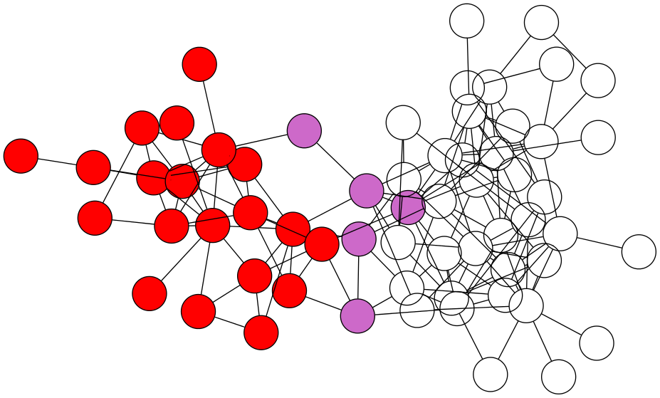
Figure 1: A communication network of agents where the leaders (in purple) have fixed decisions and the followers (in red) compute their decisions based on the leaders and the subnetwork of followers. The local solution would be the decisions of the followers.

3 Solving Local Laplacian Linear Systems with a Boundary Condition

For a general connected, simple graph $G$ and a subset of vertices $S$, consider the linear system $\mathcal{L}x=b,$ where the vector $b$ has non-empty support on the vertex boundary of $S$. The global problem is finding a solution $x$ that agrees with $b$, in the sense that $x(v)=b(v)$ for every vertex $b$ in the support of $b$. In this case we say that $x$ satisfies the boundary condition $b$.

Specifically, for a vector $b\in\mathbb{R}^{V}$, let $S$ denote a subset of vertices in the complement of $\textmd{supp}(b)$. Then $b$ can be viewed as a function defined on the vertex boundary $\delta(S)$ of $S$ and we say $b$ is a boundary condition of $S$. Here we will consider the case that the induced subgraph on $S$ is connected.

Definition 1.

Let $G$ be a graph and let $b$ be a vector $b\in\mathbb{R}^{V}$ over the vertices of $G$ with non-empty support. Then we say a subset of vertices $S\subset V$ is a $b$-boundable subset if

1. $S\subseteq V\setminus\textmd{supp}(b)$,

2. $\delta(S)\cap\textmd{supp}(b)\neq\emptyset$,

3. the induced subgraph on $S$ is connected and $\delta(S)\neq\emptyset$.

We note that condition (iii) is required in our analysis later, although the general problem of finding a local solution over $S$ can be dealt with by solving the problem on each connected component of the induced subgraph on $S$ individually. We remark that in this setup, we do not place any condition on $b$ beyond having non-empty support. The entries in $b$ may be positive or negative.

The global solution to the system $\mathcal{L}x=b$ satisfying the boundary condition $b$ is a vector $x\in\mathbb{R}^{V}$ with

$$x(v)=\begin{cases}\sum\limits_{u\sim v}\frac{x(u)}{\sqrt{d_{v}d_{u}}}&~{}\text{if}~{}v\in S\\ b(v)&~{}\text{if}~{}v\not\in S\end{cases}$$ (1)

for a $b$-boundable subset $S$. The problem of interest is computing the local solution for the restriction of $x$ to the subset $S$, denoted $x_{S}$.

The eigenvalues of $\mathcal{L}_{S}$ are called Dirichlet eigenvalues, denoted $\lambda_{1}\leq\lambda_{2}\leq\cdots\leq\lambda_{s}$ where $s=|S|$. It is easy to check (see [4]) that $0<\lambda_{i}\leq 2$ since we assume $\delta(S)\neq\emptyset$. Thus $\mathcal{L}_{S}^{-1}$ exists and is well defined. In fact, $s^{-3}<\lambda_{1}\leq 1$.

Let $A_{S,\delta S}$ be the $s\times|\delta(S)|$ matrix by restricting the columns of $A$ to $\delta(S)$ and rows to $S$. Requiring $S$ to be a $b$-boundable subset ensures that the inverse $\mathcal{L}_{S}^{-1}$ exists [4]. Then the local solution is described exactly in the following theorem.

Theorem 3.1.

In a graph $G$, suppose $b$ is a nontrivial vector in $\mathbb{R}^{V}$ and $S$ is a $b$-boundable subset. Then the local solution to the linear system $\mathcal{L}x=b$ satisfying the boundary condition $b$ satisfies

$$x_{S}=\mathcal{L}_{S}^{-1}(D_{S}^{-1/2}A_{S,\delta S}D_{\delta S}^{-1/2}b_{\delta S}).$$ (2)

Proof.

The vector $b_{1}:=D_{S}^{-1/2}A_{\delta S}D_{\delta S}^{-1/2}b_{\delta S}$ is defined over the vertices of $S$, and giveover the vertices of $S$ by

$$b_{1}(v)=\sum\limits_{u\in\delta(S),u\sim v}\frac{b(u)}{\sqrt{d_{v}d_{u}}}.$$ (3)

Also, the vector $\mathcal{L}_{S}x_{S}$ is given by, for $v\in S$,

$$\mathcal{L}_{S}x_{S}(v)=x(v)-\sum\limits_{u\in S,u\sim v}\frac{x(u)}{\sqrt{d_{v}d_{u}}}.$$ (4)

By (1) and (2), we have

$$x_{S}(v)=\sum\limits_{u\in S,u\sim v}\frac{x(u)}{\sqrt{d_{v}d_{u}}}+\sum\limits_{u\in\delta(S),u\sim v}\frac{b(u)}{\sqrt{d_{v}d_{u}}},$$

and combining (3) and (4), we have that $x_{S}=\mathcal{L}_{S}^{-1}b_{1}$. ∎

3.1 Solving the local system with Green’s function

For the remainder of this paper we are concerned with the local solution $x_{S}$. We focus our discussion on the restricted space using the assumptions that the induced subgraph on $S$ is connected and that $\delta(S)\neq\emptyset$. In particular, we consider the Dirichlet heat kernel, which is the heat kernel pagerank restricted to $S$.

The Dirichlet heat kernel is written by $\mathcal{H}_{S,t}$ and is defined as $\mathcal{H}_{S,t}=e^{-t\mathcal{L}_{S}}$. It is the symmetric version of $H_{S,t}$, where $H_{S,t}=e^{-t\Delta_{S}}=D_{S}^{-1/2}\mathcal{H}_{S,t}D_{S}^{1/2}$.

The spectral decomposition of $\mathcal{L}_{S}$ is

$$\mathcal{L}_{S}=\sum_{i=1}^{s}\lambda_{i}\mathbb{P}_{i},$$

where $\mathbb{P}_{i}$ are the projections to the $i$th orthonormal eigenvectors. The Dirichlet heat kernel can be expressed as

$$\mathcal{H}_{S,t}=\sum\limits_{i=1}^{s}e^{-t\lambda_{i}}\mathbb{P}_{i}.$$

Let $\mathcal{G}$ denote the inverse of $\mathcal{L}_{S}$. Namely, $\mathcal{G}\mathcal{L}_{S}=\mathcal{L}_{S}\mathcal{G}=I_{S}$. Then

$$\mathcal{G} =\sum_{i=1}^{s}\frac{1}{\lambda_{i}}\mathbb{P}_{i}.$$ (5)

From (5), we see that

$$\frac{1}{2}\leq||\mathcal{G}||\leq\frac{1}{\lambda_{1}},$$ (6)

where $||\cdot||$ denotes the spectral norm. We call $\mathcal{G}$ the Green’s function, and $\mathcal{G}$ can be related to $\mathcal{H}_{S,t}$ as follows:

Lemma 1.

Let $\mathcal{G}$ be the Green’s function of a connected induced subgraph on $S\subset V$ with $s=|S|$. Let $\mathcal{H}_{S,t}$ be the Dirichlet heat kernel with respect to $S$. Then

$$\mathcal{G}=\int_{0}^{\infty}\mathcal{H}_{S,t}~{}\mathrm{d}t.$$

Proof.

By our definition of the heat kernel,

$$\int_{0}^{\infty}\mathcal{H}_{S,t}~{}\mathrm{d}t =\int_{0}^{\infty}\Big{(}\sum\limits_{i=1}^{s}e^{-t\lambda_{i}}\mathbb{P}_{i}\Big{)}\mathrm{d}t$$

$$=\sum\limits_{i=1}^{s}\Big{(}\int_{0}^{\infty}e^{-t\lambda_{i}}\,\mathrm{d}t\Big{)}\mathbb{P}_{i}$$

$$=\sum\limits_{i=1}^{s}\frac{1}{\lambda_{i}}\mathbb{P}_{i}$$

$$=\mathcal{G}.$$

∎

Equipped with the Green’s function, the solution (2) can be expressed in terms of the Dirichlet heat kernel. As a corollary to Theorem 3.1 we have the following.

Corollary 1.

In a graph $G$, suppose $b$ is a nontrivial vector in $\mathbb{R}^{V}$ and $S$ is a $b$-boundable subset. Then the local solution to the linear system $\mathcal{L}x=b$ satisfying the boundary condition $b$ can be written as

$$x_{S}=\int_{0}^{\infty}\mathcal{H}_{S,t}b_{1}~{}\mathrm{d}t,$$ (7)

where $b_{1}=D_{S}^{-1/2}A_{S,\delta S}D_{\delta S}^{-1/2}b_{\delta S}$.

The computation of $b_{1}$ takes time proportional to the size of the edge boundary.

4 A Local Linear Solver Algorithm with Heat Kernel Pagerank

In the previous section, we saw how the local solution $x_{S}$ to the system satisfying the boundary condition $b$ can be expressed in terms of integrals of Dirichlet heat kernel in (7). In this section, we will show how these integrals can be well-approximated by sampling a finite number of values of Dirichlet heat kernel (Theorem 4.1) and Dirichlet heat kernel pagerank (Corollary 2). All norms $||\cdot||$ in this section are the $L_{2}$ norm.

Theorem 4.1.

Let $G$ be a graph and $\mathcal{L}$ denote the normalized Laplacian of $G$. Let $b$ be a nontrivial vector $b\in\mathbb{R}^{V}$ and $S$ a $b$-boundable subset, and let $b_{1}=D_{S}^{-1/2}A_{S,\delta S}D_{\delta S}^{-1/2}b_{\delta S}$. Then the local solution $x_{S}$ to the linear system $\mathcal{L}x=b$ satisfying the boundary condition $b$ can be computed by sampling $\mathcal{H}_{S,t}b_{1}$ for $r=\gamma^{-2}\log(s\gamma^{-1})$ values. If $\hat{x}_{S}$ is the output of this process, the result has error bounded by

$$||x_{S}-\hat{x}_{S}||=O\big{(}\gamma(||b_{1}||+||x_{S}||)\big{)}$$

with probability at least $1-\gamma$.

We prove Theorem 4.1 in two steps. First, we show how the integral (7) can be expressed as a finite Riemann sum without incurring much loss of accuracy in Lemma 2. Second, we show in Lemma 3 how this finite sum can be well-approximated by its expected value using a concentration inequality.

Lemma 2.

Let $x_{S}$ be the local solution to the linear system $\mathcal{L}x=b$ satisfying the boundary condition $b$ given in (7). Then, for $T=s^{3}\log(s^{3}\gamma^{-1})$ and $N=T/\gamma$, the error incurred by taking a right Riemann sum is

$$||x_{S}-\sum\limits_{j=1}^{N}\mathcal{H}_{S,jT/N}\frac{T}{N}b_{1}||\leq\gamma(||b_{1}||+||x_{S}||),$$

where $b_{1}=D_{S}^{-1/2}A_{S,\delta S}D_{\delta S}^{-1/2}b_{\delta S}$.

Proof.

First, we see that:

$$||\mathcal{H}_{S,t}|| =||\sum\limits_{i}e^{-t\lambda_{i}}\mathbb{P}_{i}||$$

$$\leq e^{-t\lambda_{1}}||\sum\limits_{i}\mathbb{P}_{i}||$$

$$=e^{-t\lambda_{1}}$$ (8)

where $\lambda_{i}$ are Dirichlet eigenvalues for the induced subgraph $S$. So the error incurred by taking a definite integral up to $t=T$ to approximate the inverse is the difference

$$||x_{S}-\int_{0}^{T}\mathcal{H}_{S,t}b_{1}~{}\mathrm{d}t|| =||\int_{T}^{\infty}\mathcal{H}_{S,t}b_{1}~{}\mathrm{d}t||$$

$$\leq\int_{T}^{\infty}e^{-t\lambda_{1}}||b_{1}||~{}\mathrm{d}t$$

$$\leq\frac{1}{\lambda_{1}}e^{-T\lambda_{1}}||b_{1}||.$$

Then by the assumption on $T$ the error is bounded by $||x_{S}-\int_{0}^{T}\mathcal{H}_{S,t}b_{1}~{}\mathrm{d}t||\leq\gamma||b_{1}||$.

Next, we approximate the definite integral in $[0,T]$ by discretizing it. That is, for a given $\gamma$, we choose $N=T/\gamma$ and divide the interval $[0,T]$ into $N$ intervals of size $T/N$. Then a finite Riemann sum is close to the definite integral:

$$||\int_{0}^{T}\mathcal{H}_{S,t}b_{1}~{}\mathrm{d}t-\sum\limits_{j=1}^{N}\mathcal{H}_{S,jT/N}b_{1}\frac{T}{N}|| \leq\gamma||\int_{0}^{T}\mathcal{H}_{S,t}b_{1}~{}\mathrm{d}t||$$

$$\leq\gamma||x_{S}||.$$

This gives a total error bounded by $\gamma(||b_{1}||+||x_{S}||)$. ∎

Lemma 3.

The sum $\sum\limits_{j=1}^{N}\mathcal{H}_{S,jT/N}b_{1}\frac{T}{N}$ can be approximated by sampling $r=\gamma^{-2}\log(s\gamma^{-1})$ values of $\mathcal{H}_{S,jT/N}b_{1}$ where $j$ is drawn from $[1,N]$. With probability at least $1-\gamma$, the result has multiplicative error at most $\gamma$.

A main tool in our proof of Lemma 3 is the following matrix concentration inequality (see [5], also variations in [1], [9], [20], [12], [25]).

Theorem 4.2.

Let $X_{1},X_{2},\dots,X_{m}$ be independent random $n\times n$ Hermitian matrices. Moreover, assume that $\|X_{i}-\mathbb{E}(X_{i})\|\leq M$ for all $i$, and put $v^{2}=\|\sum_{i}\text{var}(X_{i})\|$. Let $X=\sum_{i}X_{i}$. Then for any $a>0$,

$$\mathrm{Pr}(\|X-\mathbb{E}(X)\|>a)\leq 2n\exp\left(-\frac{a^{2}}{2v^{2}+2Ma/3}\right),$$

where $||\cdot||$ denotes the spectral norm.

Proof of Lemma 3.

Suppose without loss of generality that $||b_{1}||=1$. Let $Y$ be a random variable that takes on the vector $\mathcal{H}_{S,jT/N}b_{1}$ for every $j\in[1,N]$ with probability $1/N$. Then $\mathbb{E}(Y)=\frac{1}{N}\sum\limits_{j=1}^{N}\mathcal{H}_{S,jT/N}b_{1}$. Let $X=\sum\limits_{i=1}^{r}X_{j}$ where each $X_{j}$ is a copy of $Y$, so that $\mathbb{E}(X)=r\mathbb{E}(Y)$.

Now consider $\mathbb{Y}$ to be the random variable that takes on the projection matrix $\mathcal{H}_{S,jT/N}b_{1}(\mathcal{H}_{S,jT/N}b_{1})^{T}$ for every $j\in[1,N]$ with probability $1/N$, and $\mathbb{X}$ is the sum of $r$ copies of $\mathbb{Y}$. Then we evaluate the expected value and variance of $\mathbb{X}$ as follows:

$$||\mathbb{E}(\mathbb{X})|| = r||\mathbb{E}(\mathbb{Y})||$$

$$||\textmd{Var}(\mathbb{X})|| = r||\textmd{Var}(\mathbb{Y})||\leq||\frac{r}{N}\sum_{j=1}^{N}\mathcal{H}_{S,jT/N}b_{1}(\mathcal{H}_{S,jT/N}b_{1})^{T}||\mathcal{H}_{S,jT/N}b_{1}||^{2}||$$

$$\leq r||\mathbb{E}(\mathbb{Y})||.$$

We now apply Theorem 4.2 to $\mathbb{X}$. We have

$$\mathrm{Pr}\big{(}||\mathbb{X}-\mathbb{E}(\mathbb{X})||\geq\gamma||\mathbb{E}(\mathbb{X})||\big{)} \leq 2s\exp\left(-\frac{\gamma^{2}||\mathbb{E}(\mathbb{X})||^{2}}{2\textmd{Var}(\mathbb{X})+\frac{2\gamma||\mathbb{E}(\mathbb{X})||M}{3}}\right)$$

$$\leq 2s\exp\left(-\frac{\gamma^{2}r^{2}||\mathbb{E}(\mathbb{Y})||}{r+2\gamma rM/3}\right)$$

$$\leq 2s\exp\left(-\frac{\gamma^{2}r}{2}\right).$$

Therefore we have $\mathrm{Pr}\big{(}||\mathbb{X}-\mathbb{E}(\mathbb{X})||\geq\gamma||\mathbb{E}(\mathbb{X})||\big{)}\leq\gamma$ if we choose $r\geq\gamma^{-2}\log(s\gamma^{-1})$. Further, this implies the looser bound:

$$\mathrm{Pr}\big{(}||X-\mathbb{E}(X)||\geq\gamma||\mathbb{E}(X)||\big{)}\leq\gamma.$$

Then $\mathbb{E}(Y)=\frac{1}{r}\mathbb{E}(X)$ is close to $\frac{1}{r}X$ and

$$||\sum\limits_{j=1}^{N}\mathcal{H}_{S,jT/N}b_{1}\frac{1}{N}-\frac{1}{r}X|| \leq\gamma||\sum\limits_{j=1}^{N}\mathcal{H}_{S,jT/N}b_{1}\frac{1}{N}||$$

$$||\sum\limits_{j=1}^{N}\mathcal{H}_{S,jT/N}b_{1}\frac{T}{N}-\frac{T}{r}X|| \leq\gamma||\sum\limits_{j=1}^{N}\mathcal{H}_{S,jT/N}b_{1}\frac{T}{N}||$$

with probability at least $1-\gamma$, as claimed. ∎

Proof of Theorem 4.1.

Let $X$ be the sum of $r$ samples of $\mathcal{H}_{S,jT/N}b_{1}$ with $j$ drawn from $[0,N]$, and let $\hat{x}_{S}=\frac{T}{r}X$. Then combining Lemmas 2 and 3, we have

$$||x_{S}-\hat{x}_{S}|| \leq\gamma\big{(}||b_{1}||+||x_{S}||+||\sum\limits_{j=1}^{N}\mathcal{H}_{S,jT/N}b_{1}\frac{T}{N}||\big{)}$$

$$\leq O\big{(}\gamma(||b_{1}||+||x_{S}||)\big{)}.$$

By Lemma 3, this bound holds with probability at least $1-\gamma$ . ∎

The above analysis allows us to approximate the solution $x_{S}$ by sampling $\mathcal{H}_{S,t}b_{1}$ for various $t$. The following corollary is similar to Theorem 4.1 except we use the asymmetric version of the Dirichlet heat kernel which we will need later for using random walks. In particular, we use Dirichlet heat kernel pagerank vectors. Dirichlet heat kernel pagerank is also defined in terms of a subset $S$ whose induced subgraph is connected, and a vector $f\in\mathbb{R}^{S}$ by the following:

$$\rho_{S,t,f}=f^{T}H_{S,t}.$$ (9)

Corollary 2.

Let $G$ be a graph and $\mathcal{L}$ denote the normalized Laplacian of $G$. Let $b$ be a nontrivial vector $b\in\mathbb{R}^{V}$ and $S$ be a $b$-boundable subset. Let $b_{2}=(D_{S}^{-1/2}A_{S,\delta S}D_{\delta S}^{-1/2}b_{\delta S})^{T}D_{S}^{1/2}$. Then the local solution $x_{S}$ to the linear system $\mathcal{L}x=b$ satisfying the boundary condition $b$ can be computed by sampling $\rho_{S,t,b_{2}}$ for $r=\gamma^{-2}\log(s\gamma^{-1})$ values. If $\hat{x}_{S}$ is the output of this process, the result has error bounded by

$$||x_{S}-\hat{x}_{S}||=O\big{(}\gamma(||b_{1}||+||x_{S}||)\big{)},$$

where $b_{1}=D_{S}^{-1/2}A_{\delta S}D_{\delta S}^{-1/2}b_{\delta S}$, with probability at least $1-\gamma$.

Proof.

First, we show how $x_{S}$ can be given in terms of Dirichlet heat kernel pagerank.

$$x_{S}^{T} =\int_{0}^{\infty}b_{1}^{T}\mathcal{H}_{S,t}~{}\mathrm{d}t$$

$$=\int_{0}^{\infty}b_{1}^{T}(D_{S}^{1/2}H_{S,t}D_{S}^{-1/2})~{}\mathrm{d}t$$

$$=\int_{0}^{\infty}b_{2}H_{S,t}D_{S}^{-1/2}~{}\mathrm{d}t,~{}~{}\mbox{ where }b_{2}=b_{1}^{T}D_{S}^{1/2}$$

$$=\int_{0}^{\infty}\rho_{S,t,b_{2}}~{}\mathrm{d}t~{}D_{S}^{-1/2},$$

and we have an expression similar to (7). Then by Lemma 2, $x_{S}^{T}$ is close to $\sum\limits_{j=1}^{N}\rho_{S,jT/N,b_{2}}\frac{T}{N}D_{S}^{-1/2}$ with error bounded by $O\big{(}\gamma(||b_{1}||+||x_{S}||)\big{)}$. From Lemma 3, this can be approximated to within $O(\gamma||x_{S}||)$ multiplicative error using $r=\gamma^{-2}\log(s\gamma^{-1})$ samples with probability at least $1-\gamma$. This gives total additive and multiplicative error within $O(\gamma)$. ∎

4.1 The Local Linear Solver Algorithm

We present an algorithm for computing a local solution to a Laplacian linear system with a boundary condition.

Algorithm 1 Local Linear Solver

input: graph $G$, boundary vector $b\in\mathbb{R}^{V}$, subset $S\subset V$, solver error parameter $0<\gamma<1$.
output: an approximate local solution $\mathtt{x}$ with additive and multiplicative error $\gamma$ to the local system $x_{S}=\mathcal{G}b_{1}$ satisyfing the boundary condition $b$.

1:$s\leftarrow|S|$

2:initialize a $0$-vector $\mathtt{x}$ of dimension $s$

3:$b_{1}\leftarrow D_{S}^{-1/2}A_{S,\delta S}D_{\delta S}^{-1/2}b_{\delta S}$

4:$b_{2}\leftarrow b_{1}^{T}D_{S}^{1/2}$

5:$T\leftarrow s^{3}\log(s^{3}\gamma^{-1})$

6:$N\leftarrow T/\gamma$

7:$r\leftarrow\gamma^{-2}\log(s\gamma^{-1})$

8:for $i=1$ to $r$ do

9:     draw $j$ from $[1,N]$ uniformly at random

10:     $x_{i}\leftarrow\rho_{S,jT/N,b_{2}}$

11:     $\mathtt{x}\leftarrow\mathtt{x}+x_{i}$

12:end for

13:return $T/r\cdot\mathtt{x}D_{S}^{-1/2}$

Theorem 4.3.

Let $G$ be a graph and $\mathcal{L}$ denote the normalized Laplacian of $G$. Let $b$ be a nontrivial vector $b\in\mathbb{R}^{V}$, $S$ a $b$-boundable subset, and let $b_{1}=D_{S}^{-1/2}A_{S,\delta S}D_{\delta S}^{-1/2}b_{\delta S}$. For the linear system $\mathcal{L}x=b$, the solution $x$ is required to satisfy the boundary condition $b$, and let $x_{S}$ be the local solution. Then the approximate solution $\mathtt{x}$ output by the Local Linear Solver algorithm has an error bounded by

$$||x_{S}-\mathtt{x}||=O\big{(}\gamma(||b_{1}||+||x_{S}||)\big{)}$$

with probability at least $1-\gamma$.

Proof.

The correctness of the algorithm follows from Corollary 2. ∎

The algorithm involves $r=\gamma^{-2}\log(s\gamma^{-1})$ Dirichlet heat kernel pagerank computations, so the running time is proportional to the time for computing $b_{2}e^{-T\Delta_{S}}$ for $T=s^{3}\log(s^{3}\gamma^{-1})$.

In the next sections, we discuss an efficient way to approximate a Dirichlet heat kernel pagerank vector and the resulting algorithm GreensSolver that returns approximate local solutions in sublinear time.

5 Dirichlet Heat Kernel Pagerank Approximation Algorithm

The definition of Dirichlet heat kernel pagerank in (9) is given in terms of a subset $S$ and a vector $f\in\mathbb{R}^{S}$. Our goal is to express this vector as the stationary distribution of random walks on the graph in order to design an efficient approximation algorithm.

Dirichlet heat kernel pagerank is defined over the vertices of a subset $S$ as follows:

$$\rho_{S,t,f} =f^{T}H_{S,t}=f^{T}e^{-t\Delta_{S}}=f^{T}e^{-t(I_{S}-P_{S})}$$

$$=\sum\limits_{k=0}^{\infty}e^{-t}\frac{t^{k}}{k!}f^{T}P_{S}^{k}.$$

That is, it is defined in terms of the transition probability matrix $P_{S}$ – the restriction of $P$ where $P$ describes a random walk on the graph. We can interpret the matrix $P_{S}$ as the transition probability matrix of the following so-called Dirichlet random walk: Move from a vertex $u$ in $S$ to a neighbor $v$ with probability $1/d_{u}$. If $v$ is not in $S$, abort the walk and ignore any probability movement. Since we only consider the diffusion of probability within the subset, any random walks which leave $S$ cannot be allowed to return any probability to $S$. To prevent this, random walks that do not remain in $S$ are ignored.

We recall some facts about random walks. First, if $g$ is a probabilistic function over the vertices of $G$, then $g^{T}P^{k}$ is the probability distribution over the vertices after performing $k$ random walk steps according to $P$ starting from vertices drawn from $g$. Similarly, when $f$ is a probabilistic fuction over $S$, $f^{T}P_{S}^{k}$ is the distribution after $k$ Dirichlet random walk steps. Consider a Dirichlet random walk process in which the number of steps taken, $k$ (where steps are taken according to a Dirichlet random walk as described above), is a Poisson random variable with mean $t$. That is, $k$ steps are taken with probability $p_{t}(k)=e^{-t}\frac{t^{k}}{k!}$. Then, the Dirichlet heat kernel pagerank is the expected distribution of this process.

In order to use random walks for approximating Dirichlet heat kernel pagerank, we perform some preprocessing for general vectors $f\in\mathbb{R}^{S}$. Namely, we do separate computations for the positive and negative parts of the vector, and normalize each part to be a probability distribution.

Given a graph and a vector $f\in\mathbb{R}^{S}$, the algorithm ApproxDirHKPR computes vectors that $\epsilon$-approximate the Dirichlet heat kernel pagerank $\rho_{S,t,f}$ satisfying the following criteria:

Definition 2.

Let $G$ be a graph and let $S\subset V$ be a subset of vertices. Let $f\in\mathbb{R}^{S}$ be a probability distribution vector over the vertices of $S$ and let $\rho_{S,t,f}$ be the Dirichlet heat kernel pagerank vector according to $S$, $t$ and $f$. Then we say that $\nu\in\mathbb{R}^{S}$ is an $\epsilon$-approximate Dirichlet heat kernel pagerank vector if

1. for every vertex $v$ in the support of $\nu$, $|\rho_{S,t,f}(v)-\nu(v)|\leq\epsilon\cdot\rho_{S,t,f}(v),$ and

2. for every vertex with $\nu(v)=0$, it must be that $\rho_{S,t,f}(v)\leq\epsilon$.

When $f$ is a general vector, an $\epsilon$-approximate Dirichlet heat kernel pagerank vector has an additional additive error of $\epsilon||f||_{1}$ by scaling, where $||\cdot||_{1}$ denotes the $L_{1}$ norm.

For example, the zero-vector is an $\epsilon$-approximate of any vector with all entries of value $<\epsilon$. We remark that for a vector $f$ with $L_{1}$ norm $1$, the Dirichlet heat kernel pagerank vector $\rho_{S,t,f}$ has at most $1/\epsilon$ entries with values at least $\epsilon$. Thus a vector that $\epsilon$-approximates $\rho_{S,t,f}$ has support of size at most $1/\epsilon$.

Algorithm 2 ApproxDirHKPR($G,t,f,S,\epsilon$)

input: a graph $G$, $t\in\mathbb{R}^{+}$, vector $f\in\mathbb{R}^{S}$, subset $S\subset V$, error parameter $0<\epsilon<1$.
output: $\rho$, an $\epsilon$-approximation of $\rho_{S,t,f}$.

1:$s\leftarrow|S|$

2:initialize $0$-vector $\rho$ of dimension $s$

3:$f_{+}\leftarrow$ the positive portion of $f$

4:$f_{-}\leftarrow$ the negative portion of $f$ so that $f=f_{+}-f_{-}$

5:$f_{+}^{\prime}\leftarrow f_{+}/||f_{+}||_{1}$ $\triangleright$ normalize $f_{+}$ to be a probability distribution vector

6:$f_{-}^{\prime}\leftarrow f_{-}/||f_{-}||_{1}$ $\triangleright$ normalize $f_{-}$ to be a probability distribution vector

7:$r\leftarrow\frac{16}{\epsilon^{3}}\log n$

8:for $r$ iterations do

9:     choose a starting vertex $u_{1}$ according to the distribution vector $f_{+}^{\prime}$

10:     $k\sim Poiss(t)$ $\triangleright$ choose $k$ with probability $e^{-t}\frac{t^{k}}{k!}$

11:     $k\leftarrow min\{k,t/\epsilon\}$

12:     simulate $k$ steps of a $P=D^{-1}A$ random walk

13:     if the random walk leaves $S$ then:

14:         do nothing for the rest of this iteration

15:     else

16:         let $v_{1}$ be the last vertex visited in the walk

17:         $\rho[v_{1}]\leftarrow\rho[v_{1}]+||f_{+}||_{1}$

18:     end if

19:     choose a starting vertex $u_{2}$ according to the distribution vector $f_{-}^{\prime}$

20:     $k\sim Poiss(t)$ $\triangleright$ choose $k$ with probability $e^{-t}\frac{t^{k}}{k!}$

21:     $k\leftarrow min\{k,t/\epsilon\}$

22:     simulate $k$ steps of a $P=D^{-1}A$ random walk

23:     if the random walk leaves $S$ then:

24:         do nothing for the rest of this iteration

25:     else

26:         let $v_{2}$ be the last vertex visited in the walk

27:         $\rho[v_{2}]\leftarrow\rho[v_{2}]+||g_{-}||_{1}$

28:     end if

29:end for

30:

31:$\rho\leftarrow\rho/r$

32:return $\rho$

The time complexity of ApproxDirHKPR is given in terms of random walk steps. As such, the analysis assumes access to constant-time queries returning (i) the destination of a random walk step, and (ii) a sample from a distribution.

Theorem 5.1.

Let $G$ be a graph and $S$ a proper vertex subset such that the induced subgraph on $S$ is connected. Let $f$ be a vector $f\in\mathbb{R}^{S}$, $t\in\mathbb{R}^{+}$, and $0<\epsilon<1$. Then the algorithm ApproxDirHKPR($G,t,f,S,\epsilon$)  outputs an $\epsilon$-approximate Dirichlet heat kernel pagerank vector $\hat{\rho}_{S,t,f}$ with probability at least $1-\epsilon$. The running time of ApproxDirHKPR  is $O\Big{(}\epsilon^{-4}t\log n\Big{)}$, where the constant hidden in the big-O notation reflects the time to perform a random walk step.

Our analysis relies on the usual Chernoff bounds restated below. They will be applied in a similar fashion as in [3].

Lemma 4 ([3]).

Let $X_{i}$ be independent Bernoulli random variables with $X=\sum\limits_{i=1}^{r}X_{i}$. Then,

1. for $0<\epsilon<1$, $\mathrm{Pr}(X<(1-\epsilon)r\mathbb{E}(X))<\exp(-\frac{\epsilon^{2}}{2}r\mathbb{E}(X))$

2. for $0<\epsilon<1$, $\mathrm{Pr}(X>(1+\epsilon)r\mathbb{E}(X))<\exp(-\frac{\epsilon^{2}}{4}r\mathbb{E}(X))$

3. for $c\geq 1$, $\mathrm{Pr}(X>(1+c)r\mathbb{E}(X))<\exp(-\frac{c}{2}r\mathbb{E}(X))$.

Proof of Theorem 5.1.

For the sake of simplicity, we provide analysis for the positive part of the vector, $f:=f_{+}$, noting that it is easily applied similarly to the negative part as well.

The vector $f^{\prime}=f/||f||_{1}$ is a probability distribution and the heat kernel pagerank $\rho^{\prime}_{S,t,f}=\rho_{S,t,f}/||f||_{1}$ can be interpreted as a series of Dirichlet random walks in which, with probability $e^{-t}\frac{t^{k}}{k!}$, $f^{\prime T}P_{S}^{k}$ is contributed to $\rho^{\prime}_{S,t,f}$. This is demonstrated by examining the coefficients of the terms, since

$$e^{-t}\sum\limits_{k=0}^{\infty}\frac{t^{k}}{k!}=1.$$

The probability of taking $k\sim Pois(t)$ steps such that $k\geq t/\epsilon$ is less than $\epsilon$ by Markov’s inequality. Therefore, enforcing an upper bound of $K=t/\epsilon$ for the number of random walk steps taken is enough mixing time with probability at least $1-\epsilon$.

For $k\leq t/\epsilon$, our algorithm approximates $f^{\prime T}P_{S}^{k}$ by simulating $k$ random walk steps according to $P$ as long as the random walk remains in $S$. If the random walk ever leaves $S$, it is ignored. To be specific, let $X^{v}_{k}$ be the indicator random variable defined by $X^{v}_{k}=1$ if a random walk beginning from a vertex $u$ drawn from $f^{\prime}=f/||f||_{1}$ ends at vertex $v$ in $k$ steps without leaving $S$. Let $X^{v}$ be the random variable that considers the random walk process ending at vertex $v$ in at most $k$ steps without leaving $S$. That is, $X^{v}$ assumes the vector $X^{v}_{k}$ with probability $e^{-t}\frac{t^{k}}{k!}$. Namely, we consider the combined random walk

$$X^{v}=\sum_{k\leq t/\epsilon}e^{-t}\frac{t^{k}}{k!}X^{v}_{k}.$$

Now, let $\rho(k)_{S,t,f}$ be the contribution to the heat kernel pagerank vector $\rho_{S,t,f}^{\prime}$ of walks of length at most $k$. The expectation of each $X^{v}$ is $\rho(k)_{S,t,f}(v)$. Then, by Lemma 4,

$$\mathrm{Pr}(X^{v}<(1-\epsilon)\rho(k)_{S,t,f}(v)\cdot r) <\exp(-\rho(k)_{S,t,f}(v)r\epsilon^{2}/2)$$

$$=\exp(-(8/\epsilon)\rho(k)_{S,t,f}(v)\log n)$$

$$<n^{-4}$$

for every component with $\rho_{S,t,f}^{\prime}(v)>\epsilon$, since then $\rho(k)_{S,t,f}(v)>\epsilon/2$. Similarly,

$$\mathrm{Pr}(X^{v}>(1+\epsilon)\rho(k)_{S,t,f}(v)\cdot r) <\exp(-\rho(k)_{S,t,f}(v)r\epsilon^{2}/4)$$

$$=\exp(-(4/\epsilon)\rho(k)_{S,t,f}(v)\log n)$$

$$<n^{-2}.$$

We conclude the analysis for the support of $\rho_{S,t,f}^{\prime}$ by noting that $\hat{\rho}_{S,t,f}=\frac{1}{r}X^{v}$, and we achieve an $\epsilon$-multiplicative error bound for every vertex $v$ with $\rho_{S,t,f}^{\prime}(v)>\epsilon$ with probability at least $1-O(n^{-2})$.

On the other hand, if $\rho_{S,t,f}^{\prime}(v)\leq\epsilon$, by the third part of Lemma 4, $\mathrm{Pr}(\hat{\rho}_{S,t,f}(v)>2\epsilon)\leq n^{-8/\epsilon^{2}}$. We conclude that, with high probability, $\hat{\rho}_{S,t,f}(v)\leq 2\epsilon$.

Finally, when $f$ is not a probability distribution, the above applies to $f^{\prime}=f/||f||_{1}$. Let $\hat{\rho}_{S,t,f}^{\prime}$ be the output of the algorithm using $f^{\prime}=f/||f||_{1}$ and $\rho_{S,t,f}^{\prime}$ be the corresponding Dirichlet heat kernel pagerank vector $\rho_{S,t,f^{\prime}}$. The full error of the Dirichlet heat kernel pagerank returned is

$$||\rho_{S,t,f}-\hat{\rho}_{S,t,f}||_{1} \leq||||f||_{1}\rho_{S,t,f}^{\prime}-||f||_{1}\hat{\rho}_{S,t,f}^{\prime}||_{1}$$

$$\leq||f||_{1}||\rho_{S,t,f}^{\prime}-\hat{\rho}_{S,t,f}^{\prime}||_{1}$$

$$\leq\epsilon||f||_{1}||\rho_{S,t,f}^{\prime}||_{1}$$

$$=\epsilon||f||_{1}.$$

For the running time, we use the assumptions that performing a random walk step and drawing from a distribution with finite support require constant time. These are incorporated in the random walk simulation, which dominates the computation. Therefore, for each of the $r$ rounds, at most $K$ steps of the random walk are simulated, giving a total of $rK=O\Big{(}\frac{16}{\epsilon^{3}}\log n\cdot t/\epsilon\Big{)}=\tilde{O}(t)$ queries. ∎

6 The GreensSolver Algorithm

Here we present the main algorithm, GreensSolver, for computing a solution to a Laplacian linear system with a boundary condition. It is the Local Linear Solver algorithmic framework combined with the scheme for approximating Dirichlet heat kernel pagerank. The scheme is an optimized version of the algorithm ApproxDirHKPR with a slight modification. We call the optimized version SolverApproxDirHKPR.

Definition 3.

Define SolverApproxDirHKPR($G,t,f,S,\epsilon$) to be the algorithm ApproxDirHKPR($G,t,f,S,\epsilon$) with the following modification to lines 11 and 21 after drawing $k\sim Poiss(t)$:

$k\leftarrow min\{k,2t\}$.

Namely, this modification limits the length of random walk steps to at most $2t$.

Theorem 6.1.

Let $G$ be a graph and $S$ a subset of size $s$. Let $T=s^{3}\log(s^{3}\gamma^{-1})$, and let $N=T/\gamma$ for some $0<\gamma<1$. Suppose $j$ is a random variable drawn from $[1,\lfloor N\rfloor]$ uniformly at random and let $t=jT/N$. Then if $\epsilon\geq\gamma$, the algorithm SolverApproxDirHKPR returns a vector that $\epsilon$-approximates $\rho_{S,t,f}$ with probability at least $1-\epsilon$. Using the same query assumptions as Theorem 5.1, the running time of SolverApproxDirHKPR is $O\left(\epsilon^{-3}t\log n\right)$.

We will use the following Chernoff bound for Poisson random variables.

Lemma 5 ([19]).

Let $X$ be a Poisson random variable with parameter $t$. Then, if $x>t$,

$$\mathrm{Pr}(X\geq x)\leq e^{x-t-x\log(x/t)}.$$

Proof of Theorem 6.1.

Let $k$ be a Poisson random variable with parameter $t$. Similar to the proof of Theorem 5.1, we use Lemma 5 to reason that

$$\mathrm{Pr}(k\geq 2t) \leq e^{2t-t-2t\log(2t/t)}$$

$$=e^{t(1-2\log 2)}$$

$$\leq\epsilon,$$

as long as $t\geq\frac{\log(\epsilon^{-1})}{1-2\log 2}$.

Let $E$ be the event that $t<\frac{\log(\epsilon^{-1})}{1-2\log 2}$. The probability of $E$ is

$$\mathrm{Pr}\left(jT/N<\frac{\log(\epsilon^{-1})}{1-2\log 2}\right) =\mathrm{Pr}\left(j<\frac{\log(\epsilon^{-1})}{\gamma(1-2\log 2)}\right)$$

$$=\frac{\log(\epsilon^{-1})}{(1-2\log 2)s^{3}\log(s^{3}\gamma^{-1})},$$

which is less than $\epsilon$ as long as $\epsilon\geq\left(\frac{\gamma}{s^{3}}\right)^{(1-2\log 2)\epsilon s^{3}}$. This holds when $\epsilon\geq\gamma$.

As before, the algorithm consists of $r$ rounds of random walk simulation, where each walk is at most $2t$. The algorithm therefore makes $r\cdot 2t=\epsilon^{-3}32t\log n$ queries, requiring $O\left(\epsilon^{-3}t\log n\right)$ time. ∎

Below we give the algorithm GreensSolver. The algorithm is identical to Local Linear Solver with the exception of line 10, where we use the approximation algorithm SolverApproxDirHKPR for Dirichlet heat kernel pagerank computation.

Algorithm 3 GreensSolver($G,b,S,\gamma,\epsilon$)

input: graph $G$, boundary vector $b\in\mathbb{R}^{V}$, subset $S\subset V$, solver error parameter $0<\gamma<1$, Dirichlet heat kernel pagerank error parameter $0<\epsilon<1$.
output: an approximate local solution $\mathtt{x}$ to the local system $x_{S}=\mathcal{G}b_{1}$ satisyfing the boundary condition $b$.

1:$s\leftarrow|S|$

2:initialize a $0$-vector $\mathtt{x}$ of dimension $s$

3:$b_{1}\leftarrow D_{S}^{-1/2}A_{S,\delta S}D_{\delta S}^{-1/2}b_{\delta S}$

4:$b_{2}\leftarrow b_{1}^{T}D_{S}^{1/2}$

5:$T\leftarrow s^{3}\log(s^{3}\gamma^{-1})$

6:$N\leftarrow T/\gamma$

7:$r\leftarrow\gamma^{-2}\log(s\gamma^{-1})$

8:for $i=1$ to $r$ do

9:     draw $j$ from $[1,N]$ uniformly at random

10:     $x_{i}\leftarrow$ SolverApproxDirHKPR($G,jT/N,b_{2},S,\epsilon$)

11:     $\mathtt{x}\leftarrow\mathtt{x}+x_{i}$

12:end for

13:return $T/r\cdot\mathtt{x}D_{S}^{-1/2}$

Theorem 6.2.

Let $G$ be a graph and $\mathcal{L}$ denote the normalized Laplacian of $G$. Let $b$ be a nontrivial vector $b\in\mathbb{R}^{V}$ and $S$ a $b$-boundable subset, and let $b_{1}=D_{S}^{-1/2}A_{S,\delta S}D_{\delta S}^{-1/2}b_{\delta S}$. For the linear system $\mathcal{L}x=b$, the solution $x$ is required to satisfy the boundary condition $b$, and let $x_{S}$ be the local solution. Then the approximate solution $\mathtt{x}$ output by the algorithm GreensSolver satisfies the following:

1. The error of $\mathtt{x}$ is $||x_{S}-\mathtt{x}||=O\big{(}\gamma(||b_{1}||+||x_{S}||)+\epsilon||b_{2}||_{1}\big{)}$ with probability at least $1-\gamma$,

2. The running time of GreensSolver  is $O\left(\gamma^{-2}\epsilon^{-3}s^{3}\log^{2}(s^{3}\gamma^{-1})\log n\right)$ where the big-O constant reflects the time to perform a random walk step, plus additional preprocessing time $O(|\partial(S)|)$, where $\partial(S)$ denotes the edge boundary of $S$.

Proof.

The error of the algorithm using true Dirichlet heat kernel pagerank vectors is $O\big{(}\gamma(||b_{1}||+||x_{S}||)\big{)}$ by Corollary 2, so to prove (i) we address the additional error of vectors output by the approximation of SolverApproxDirHKPR. By Theorem 6.1, SolverApproxDirHKPR outputs an $\epsilon$-approximate Dirichlet heat kernel pagerank vector with probability at least $1-\epsilon$. Let $\hat{\rho}_{S,t,f}$ be the output of an arbitrary run of SolverApproxDirHKPR($G,t,f,S,\epsilon$). Then $||\rho_{S,t,f}-\hat{\rho}_{S,t,f}||\leq\epsilon(||\rho_{S,t,f^{\prime}}||_{1}+||f||_{1})=\epsilon||f||_{1}$ by the definition of $\epsilon$-approximate Dirichlet heat kernel pagerank vectors, where $f^{\prime}=f/||f||_{1}$ is the normalized vector $f$. This means that the total error of GreensSolver is

$$||x_{S}-\mathtt{x}||\leq O\left(\gamma(||b_{1}||+||x_{S}||)\right)+\epsilon||b_{2}||_{1}.$$

Next we prove (ii). The algorithm makes $r=\gamma^{-2}\log(s\gamma^{-1})$ sequential calls to SolverApproxDirHKPR. The maximum possible value of $t$ is $T=s^{3}\log(s^{3}\gamma^{-1})$, so any call to SolverApproxDirHKPR is bounded by $O\left(\epsilon^{-3}s^{3}\log(s^{3}\gamma^{-1})\log n\right)$. Thus, the total running time is $O\left(\gamma^{-2}\epsilon^{-3}s^{3}\log^{2}(s^{3}\gamma^{-1})\log n\right)$.

The additional preprocessing time of $O(|\partial(S)|)$ is for computing the vectors $b_{1}$ and $b_{2}$; these may be computed as a preliminary procedure. ∎

We note that the running time above is a sequential running time attained by calling SolverApproxDirHKPR $r$ times. However, by calling these in $r$ parallel processes, the algorithm has a parallel running time which is simply the same as that for SolverApproxDirHKPR.

6.1 Restricted Range for Approximation

Since SolverApproxDirHKPR only promises approximate values for vertices whose true Dirichlet heat kernel pagerank vector values are greater than $\epsilon$, the
GreensSolver algorithm can be optimized even further by preempting when this is the case.

Figure 2 illustrates how vector values drop as $t$ gets large. The network is the same example network given in Section 2.2 and is further examined in the next section. We let $t$ range from $1$ to $T=s^{3}\log(s^{3}\gamma^{-1})\approx 108739$ for $\gamma=0.01$ and compute Dirichlet heat kernel pagerank vectors $\rho_{S,t,f}$. The figure plots $L_{1}$ norms of the vectors as a solid line, and the absolute value of the maximum entry in the vector as a dashed line. In this example, no vector entry is larger than $0.01$ for $t$ as small as $250$.

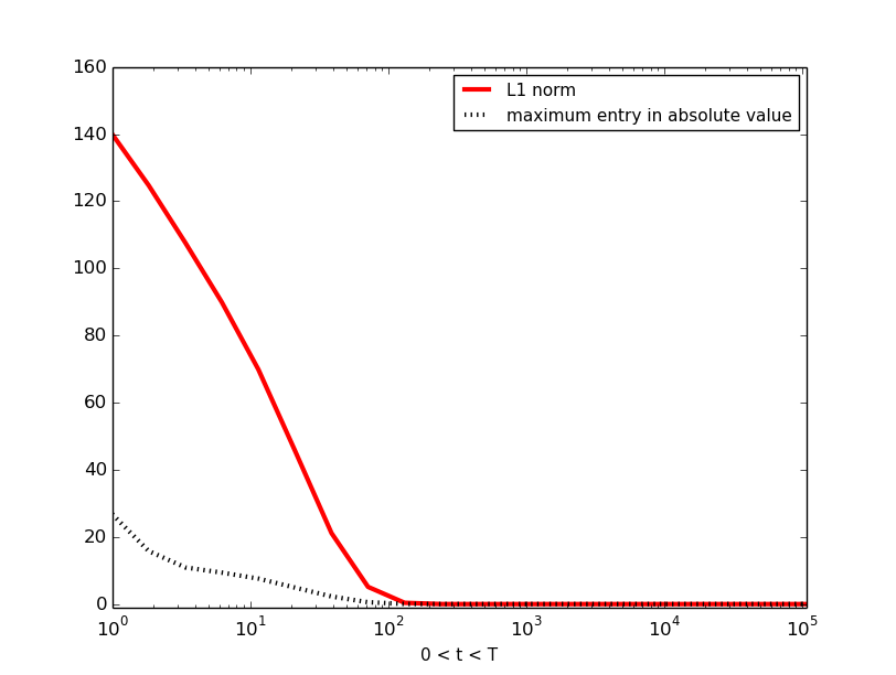
Figure 2: How support values of a Dirichlet heat kernel pagerank vector change for different values of $1\leq t\leq T=s^{3}\log(s^{3}\gamma^{-1})$. The solid line is the $L_{1}$ norm – the sum of all the support values – and the dashed line is the absolute value of the maximum entry in the vector. Note the x-axis is log-scale.

Suppose it is possible to know ahead of time whether a vector $\rho_{S,t,f}$ will have negligably small values for some value $t$. Then we could skip the computation of this vector and simply treat it as a vector of all zeros.

From (8), the norm of Dirichlet heat kernel pagerank vectors are monotone decreasing. Then it is enough to choose a threshold value $t^{\prime}$ beyond which $||\rho_{S,t^{\prime},f}||_{1}<\epsilon$, since any $\epsilon$-approximation will return all zeros, and treat this as a cutoff for actually executing the algorithm. An optimization heuristic is to only compute SolverApproxDirHKPR($G,t,f,S,\epsilon$) if $t$ is less than this threshold value $t^{\prime}$. Otherwise we can add zeros (or do nothing). That is, replace line 10 in GreensSolver with the following:

if $jT/N<t^{\prime}$ then

     $x_{i}\leftarrow$ SolverApproxDirHKPR($G,jT/N,b_{2},S,\epsilon$)

else

     do nothing

end if

From (8), a conservative choice for $t^{\prime}$ is $\frac{1}{\lambda_{1}}\log(\epsilon^{-1})$.

7 An Example Illustrating the Algorithm

We return to our example to illustrate a run of the Green’s solver algorithm for computing local linear solutions. The network is a small communication network of dolphins [18].

In this example, the subset has a good cluster, which makes it a good candidate for an algorithm in which computations are localized. Namely, it is ideal for SolverApproxDirHKPR, which promises good approximation for vertices that exceed a certain support threshold in terms of the error parameter $\epsilon$. The support of the vector $b$ is limited to the set of leaders, which is the vertex boundary of the subset of followers, $l=\delta(f)$. The vector is plotted over the agents (vertices) in Figure 3.

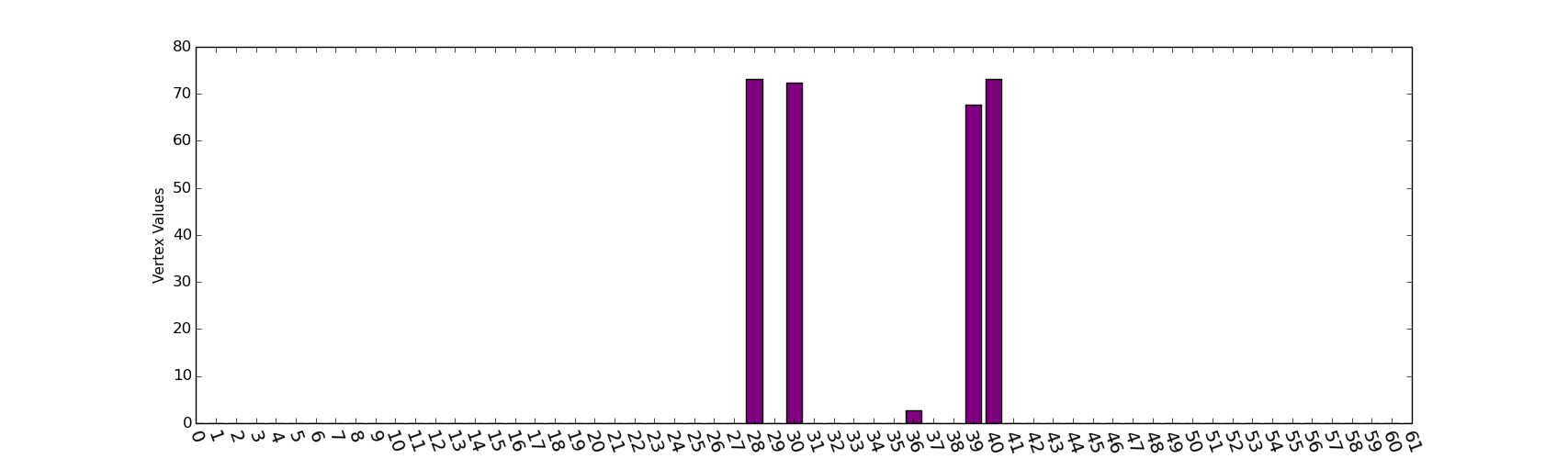
Figure 3: The values of the boundary vector plotted against the agent IDs given in Figure 1.

Figure 4 plots the vector values of the heat kernel pagerank vector $\rho_{t,b_{2}^{\prime}}$ over the full set of agents. Here, we use $b_{2}^{\prime}$, the $n$-dimensional vector:

$$b_{2}^{\prime}(v)=\begin{cases}b_{2}(v)\mbox{ if $v\in S$,}\\ 0\mbox{ otherwise,}\end{cases}$$

and $t=50.0$. The components with largest absolute value are concentrated in the subset of followers over which we compute the local solution. This indicates that an output of SolverApproxDirHKPR will capture these values well.

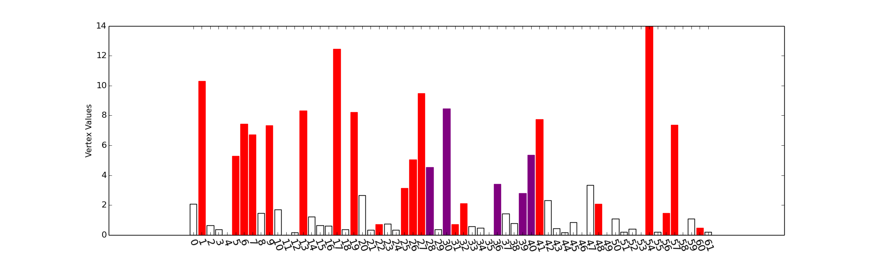
Figure 4: The node values of the full example communication network over a sample heat kernel pagerank vector. The red bars correspond to the network of followers, the purple to the leaders, and the white to the rest of the network.

7.1 Approximate solutions

In the following figures, we plot the results of calls to our approximation algorithms against the exact solution $x_{S}$ using the boundary vector of Figure 3. The solution $x_{S}$ is computed by Theorem 3.1, and the appromimations are sample outputs of Local Linear Solverand GreensSolver, respectively. The exact values of $x_{S}$ are represented by circles, and the approximate values by triangles in each case. Note that we permute the indices of the vertices in the solutions so that vector values in the exact solution, $x_{S}$ are decreasing, for reading ease.

The result of a sample call to Local Linear Solver with error parameter $\gamma=0.01$ is plotted in Figure 5. The total relative error of this solution is $\frac{||x_{S}-\hat{x}_{S}||}{||x_{S}||}=0.02$, and the absolute error $||x_{S}-\hat{x}_{S}||$ is within the error bounds given in Theorem 4.3. That is, $||x_{S}-\hat{x}_{S}||\leq\gamma\left(||b_{1}||+||x_{S}||+||x_{rie}||\right)$, where $x_{rie}$ is the solution obtained by computing the full Riemann sum (as in Lemma 2).

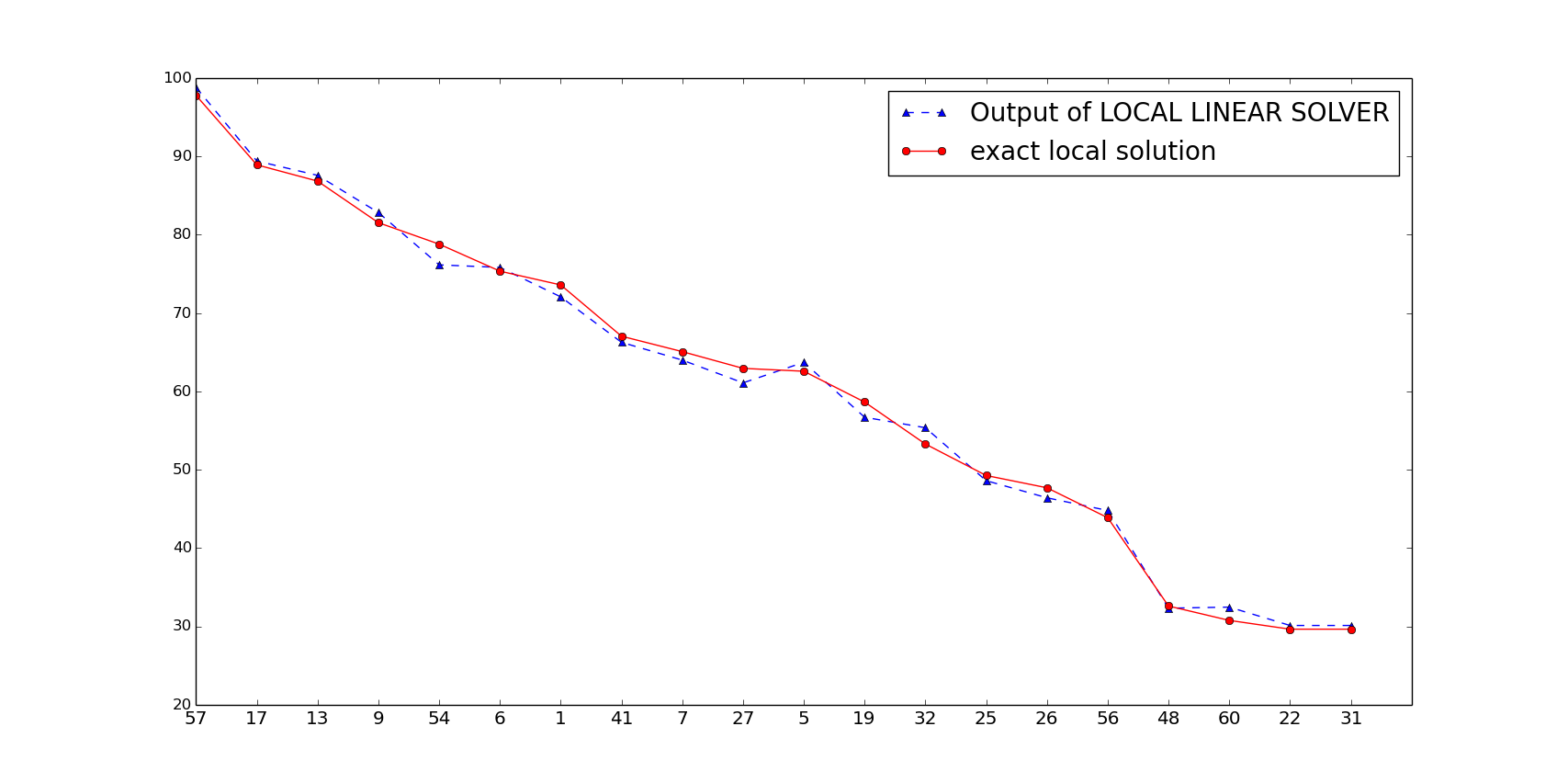
Figure 5: The results of a run of Local Linear Solver. Two vectors are plotted over IDs of agents in the subset. The circles are exact values of $x_{S}$, while the triangles are the approximate values returned by Local Linear Solver.

The result of a sample call to GreensSolver with parameters $\gamma=0.01,\epsilon=0.1$ is plotted in Figure 6. In this case the relative error is $\approx 2.05$, but the absolute error meets the error bounds promised in Theorem 6.2 point (i). Specifically,

$$||x_{S}-\hat{x}_{S}||\leq\left(\gamma(||b_{1}||+||x_{S}||+||x_{rie}||)+\epsilon||b_{2}||_{1}\right).$$

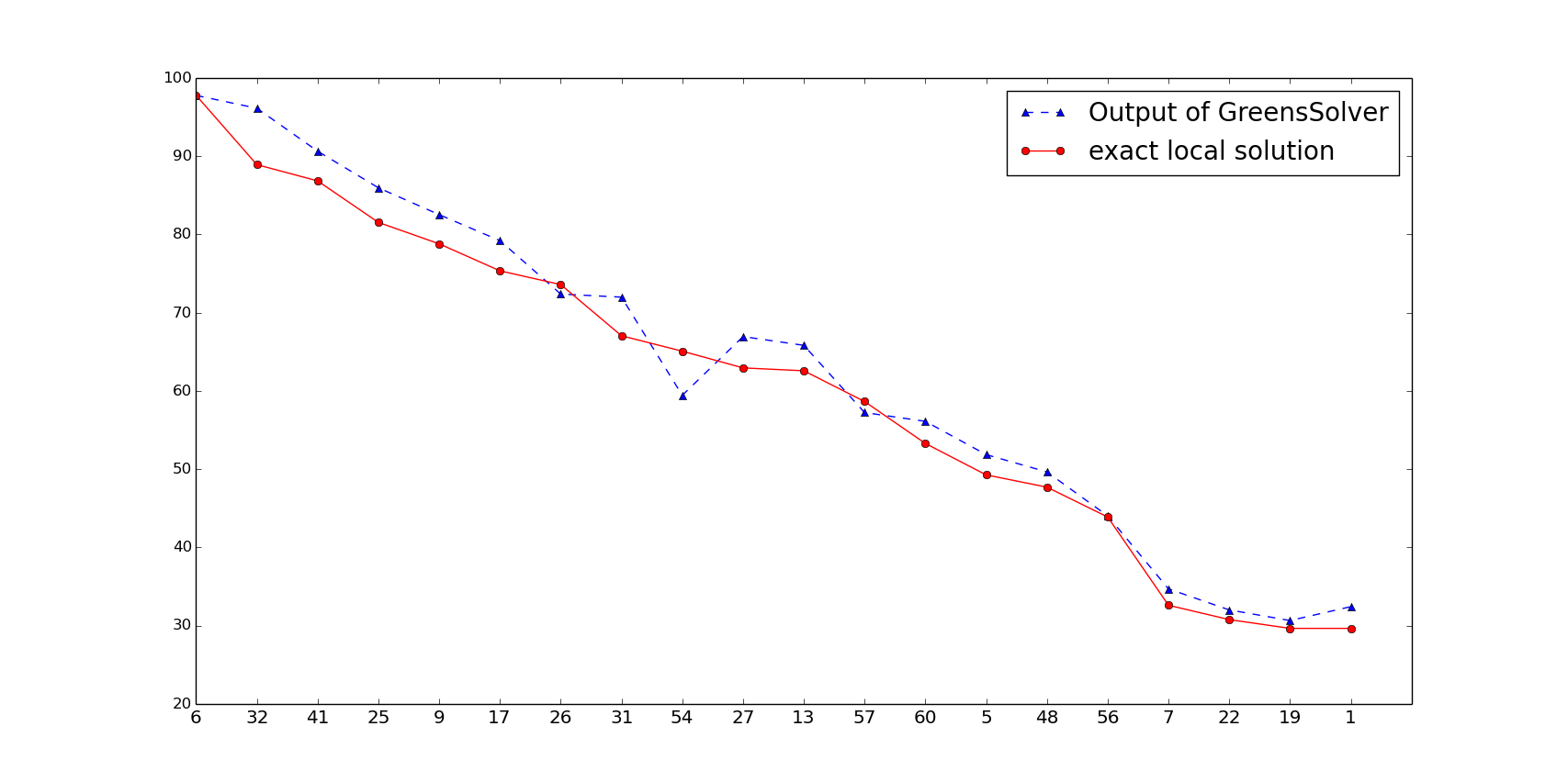
Figure 6: The results of a run of GreensSolver with $\gamma=0.01,\epsilon=0.1$.

General remarks.

While we have focused our analysis on solving local linear systems with the normalized Laplacian $\mathcal{L}$ as the coefficient matrix, our methods can be extended to solve local linear systems expressed in terms of the Laplacian $L$ as well. There are numerous applications involving solving such linear systems. Some examples are discussed in [6], and include computing effective resistance in electrical networks, computing maximum flow by interior point methods, describing the motion of coupled oscillators, and computing state in a network of communicating agents. In addition, we expect the method of approximating Dirichlet heat kernel pagerank in its own right to be useful in a variety of related applications.

Acknowledgements.

The authors would like to thank the anonymous reviewers for their comments and suggestions. Their input has been immensely helpful in improving the presentation of the results and clarifying details of the algorithm.

References

- [1] Rudolf Ahlswede and Andreas Winter, Strong converse for identification via quantum channels, IEEE Trans. Inform. Theory 48 (2002), no. 3, 569–579.
- [2] Guy E. Blelloch, Anupam Gupta, Ioannis Koutis, Gary L. Miller, and Richard Peng, Near linear-work parallel sdd solvers, low-diameter decomposition, and low-stretch subgraphs, Proceedings of the 23th ACM Symposium on Parallelism in Algorithms and Architectures, ACM, 2011, pp. 13–22.
- [3] Christian Borgs, Michael Brautbar, Jennifer T. Chayes, and Shang-Hua Teng, A sublinear time algorithm for pagerank computations, WAW (2012), 41–53.
- [4] Fan Chung, Spectral graph theory, American Mathematical Society, 1997.
- [5] Fan Chung and Mary Radcliffe, On the spectra of general random graphs, The Electronic Journal of Combinatorics 18 (2011), P215.
- [6] Fan Chung and Olivia Simpson, Solving linear systems with boundary conditions using heat kernel pagerank, Algorithms and Models for the Web Graph, 2013, pp. 203 – 219.
- [7] , Computing heat kernel pagerank and a local clustering algorithm, Proceedings of the 25th International Workshop on Combinatorial Algorithms, 2014, p. forthcoming.
- [8] Michael B. Cohen, Rasmus Kyng, Gary L. Miller, Jakub W. Pachocki, Richard Peng, Anup Rao, and Shen Chen Xu, Solving sdd linear systems in nearly time, STOC, 2014.
- [9] Demetres Cristofides and Klas Markström, Expansion properties of random cayley graphs and vertex transitive graphs via matrix martingales, Random Structures Algs. 32 (2008), no. 8, 88–100.
- [10] George E. Forsythe and Richard A. Leibler, Matrix inversion by a monte carlo method, Mathematical Tables and Other Aids to Computation 4 (1950), no. 31, 127–129.
- [11] Keith D. Gremban, Gary L. Miller, and Marco Zagha, Performance evaluation of a new parallel preconditioner, Proceedings of the 9th International Parallel Processing Symposium, IEEE, 1995, pp. 65–69.
- [12] David Gross, Recovering low-rank matrices from few coefficients in any basis, IEEE Trans. Inform. Theory 57 (2011), 1548–1566.
- [13] Jonathan A Kelner, Lorenzo Orecchia, Aaron Sidford, and Zeyuan Allen Zhu, A simple, combinatorial algorithm for solving sdd systems in nearly-linear time, STOC (2013), 911–920.
- [14] Ioannis Koutis and Gary L. Miller, A linear work time algorithm for solving planar laplacians, Proceedings of the 18th Annual ACM-SIAM Symposium on Discrete Algorithms, ACM-SIAM, 2007, pp. 1002–1011.
- [15] Ioannis Koutis, Gary L. Miller, and Richard Peng, Approaching optimality for solving sdd linear systems, FOCS (2010), 235–244.
- [16] , A nearly-m log n time solver for sdd linear systems, FOCS (2011), 590–598.
- [17] Yin Tat Lee and Aaron Sidford, Efficient accelerated coordinate descent methods and faster algorithms for solving linear systems, FOCS (2013).
- [18] D. Lusseau, K. Schneider, O.J Boisseau, P. Haase, E. Slooten, and S.M. Dawson, The bottlenose dolphin community of doubtful sound features a large proportion of long-lasting associations, Behavioral Ecology and Sociobioloy 54 (2003), 396–405.
- [19] Michael Mitzenmacher and Eli Upfal, Probability and computing: Randomized algorithms and probabilistic analysis, Cambridge University Press, 2005.
- [20] Roberto Imbuzeiro Oliveira, Concentration of the adjacency matrix and of the laplacian in random graphs with independent edges, arXiv preprint arXiv:0911.0600 (2009).
- [21] Richard Peng and Daniel A. Spielman, An efficient parallel solver for sdd linear systems, arXiv:1311.3286, November 2013.
- [22] Sushant Sachdeva and Nisheeth K. Vishnoi, Matrix inversion is as easy as exponentiation, arXiv preprint arXiv:1305.0526 (2013).
- [23] Daniel A. Spielman, Algorithms, graph theory, and linear equations in laplacian matrices, Proceedings of the International Congress of Mathematicians 4 (2010), 2698–2722.
- [24] Daniel A. Spielman and Shang-Hua Teng, Nearly-linear time algorithms for graph partitioning, graph sparsification, and solving linear systems, STOC (2004), 81–90.
- [25] Joel A Tropp, User-friendly tail bounds for sums of random matrices, Foundations of Computational Mathematics 12 (2012), no. 4, 389–434.
- [26] Pravin M Vaidya, Solving linear equations with symmetric diagonally dominant matrices by constructing good preconditioners, A talk based on this manuscript 2 (1991), no. 3.4, 2–4.
- [27] Nisheeth K. Vishnoi, Lx= b (laplacian solvers and their algorithmic applications), vol. 8, 2013.