Computing Heat Kernel Pagerank and a Local Clustering Algorithm

Abstract

Heat kernel pagerank is a variation of Personalized PageRank given in an exponential formulation. In this work, we present a sublinear time algorithm for approximating the heat kernel pagerank of a graph. The algorithm works by simulating random walks of bounded length and runs in time $O\big{(}\frac{\log(\epsilon^{-1})\log n}{\epsilon^{3}\log\log(\epsilon^{-1})}\big{)}$, assuming performing a random walk step and sampling from a distribution with bounded support take constant time.

The quantitative ranking of vertices obtained with heat kernel pagerank can be used for local clustering algorithms. We present an efficient local clustering algorithm that finds cuts by performing a sweep over a heat kernel pagerank vector, using the heat kernel pagerank approximation algorithm as a subroutine. Specifically, we show that for a subset $S$ of Cheeger ratio $\phi$, many vertices in $S$ may serve as seeds for a heat kernel pagerank vector which will find a cut of conductance $O(\sqrt{\phi})$.

1 Introduction

In large networks, many similar elements can be identified to a single, larger entity by the process of clustering. Increasing granularity in massive networks through clustering eases operations on the network. There is a large literature on the problem of identifying clusters in a graph ([8, 37, 34, 20, 28, 29]), and the problem has found many applications. However, in a variation of the graph clustering problem we may only be interested in a single cluster near one element in the graph. For this, local clustering algorithms are of greater use.

As an example, the problem of finding a local cluster arises in protein networks. A protein-protein interaction (PPI) network has undirected edges that represent an interaction between two proteins. Given two PPI networks, the goal of the pairwise alignment problem is to identify an optimal mapping between the networks that best represents a conserved biological function. In [27], a local clustering algorithm is applied from a specified protein to identify a group similar to that protein. Such local alignments are useful for analysis of a particular component of a biological system (rather than at a systems level which will call for a global alignment). Local clustering is also a common tool for identifying communities in a network. A community is loosely defined as a subset of vertices in a graph which are more strongly connected internally than to vertices outside the subset. Properties of community structure in large, real world networks have been studied in [25], for example, where local clustering algorithms are employed for identifying communities of varying quality.

The goal of a local clustering algorithm is to identify a cluster in a graph near a specified vertex. Using only local structure avoids unnecessary computation over the entire graph. An important consequence of this are running times which are often in terms of the size of the small side of the partition, rather than of the entire graph. The best performing local clustering algorithms use probability diffusion processes over the graph to determine clusters (see Section 1.1). In this paper we present a new algorithm which identifies a cut near a specified vertex with simple computations over a heat kernel pagerank vector.

The theory behind using heat kernel pagerank for computing local clusters has been considered in previous work. Here we give an efficient approximation algorithm for computing heat kernel pagerank. Note that we use a “relaxed” notion of approximation which allows us to derive a sublinear probabilistic approximation algorithm for heat kernel pagerank, while computing an exact or sharp approximation would require computation complexity of order similar to matrix multiplication. We use this sublinear approximation algorithm for efficient local clustering.

1.1 Previous work

Heat kernel and approximation of matrix exponentials.

Heat kernel pagerank was first introduced in [9] as a variant of personalized PageRank [18]. While PageRank can be viewed as a geometric sum of random walks, the heat kernel pagerank is an exponential sum of random walks. An alternative interpretation of the heat kernel pagerank is related to the heat kernel of a graph as the fundamental solution to the heat equation. As such, it has connections with diffusion and mixing properties of graphs and has been incorporated into a number of graph algorithmic primitives.

Orecchia et al. use a variant of heat kernel random walks in their randomized algorithm for computing a cut in a graph with prescribed balance constraints [35]. A key subroutine in the algorithm is a procedure for computing $e^{-A}v$ for a positive semidefinite matrix $A$ and a unit vector $v$ in time $\tilde{O}(m)$ for graphs on $n$ vertices and $m$ edges. They show how this can be done with a small number of computations of the form $A^{-1}v$ and applying the Spielman-Teng linear solver [38]. Their main result is a randomized algorithm that outputs a balanced cut in time $O(m\operatorname{polylog}n)$. In a follow up paper, Sachdeva and Vishnoi [36] reduce inversion of positive semidefinite matrices to matrix exponentiation, thus proving that matrix exponentiation and matrix inversion are equivalent to polylog factors. In particular, the nearly-linear running time of the balanced separator algorithm depends upon the nearly-linear time Spielman-Teng solver.

Another method for approximating matrix exponentials is given by Kloster and Gleich in [22]. They use a Gauss-Southwell iteration to approximate the Taylor series expansion of the column vector $e^{P}e_{c}$ for transition probability matrix $P$ and $e_{c}$ a standard basis vector. The algorithm runs in sublinear time assuming the maximum degree of the network is $O(\log\log n)$.

Local clustering.

Local clustering algorithms were introduced in [38], where Spielman and Teng present a nearly-linear time algorithm for finding local partitions with certain balance constraints. Let $\Phi(S)$ denote the cut ratio of a subset $S$ that we will later define as the Cheeger ratio. Then, given a graph and a subset of vertices $S$ such that $\Phi(S)<\phi$ and $\textmd{vol}(S)\leq\textmd{vol}(G)/2$, their algorithm finds a set of vertices $T$ such that $\textmd{vol}(T)\geq\textmd{vol}(S)/2$ and $\Phi(T)\leq O(\phi^{1/3}\log^{O(1)}n)$ in time $O(m(\log n/\phi)^{O(1)})$. This seminal work incorporates the ideas of Lovász and Simonovitz [30, 31] on isoperimetric properties of random walks, and their algorithm works by simulating truncated random walks on the graph. Spielman and Teng later improve their approximation guarantee to $O(\phi^{1/2}\log^{3/2}n)$ in a revised version of the paper [39].

The algorithm of [38, 39] improves the spectral methods of [14] and a similar expression in [1] which use an eigenvector of the graph Laplacian to partition the vertices of a graph. However, the local approach of Spielman and Teng allows us to identify focused clusters without investigating the entire graph. For this reason, the running time of this and similar local algorithms are proportional to the size of the small side of the cut, rather than the entire graph.

Andersen et al. [3] give an improved local clustering algorithm using approximate PageRank vectors. For a vertex subset $S$ with Cheeger ratio $\phi$ and volume $k$, they show that a PageRank vector can be used to find a set with Cheeger ratio $O(\phi^{1/2}\log^{1/2}k)$. Their local clustering algorithm runs in time $O(\phi^{-1}m\log^{4}m)$. The analysis of the above process was strengthened in [2] and emphasized that vertices with higher PageRank values will be on the same side of the cut as the starting vertex.

Andersen and Peres [4] later simulate a volume-biased evolving set process to find sparse cuts. Although their approximation guarantee is the same as that of [3], their process yields a better ratio between the computational complexity of the algorithm on a given run and the volume of the output set. They call this value the work/volume ratio, and their evolving set algorithm achieves an expected ratio of $O(\phi^{-1/2}\log^{3/2}n)$. This result is improved by Gharan and Trevisan in [16] with an algorithm that finds a set of conductance at most $O(\epsilon^{-1/2}\phi^{1/2})$ and achieves a work/volume ratio of $O(\varsigma^{\epsilon}\phi^{-1/2}\log^{2}n)$ for target volume $\varsigma$ and target conductance $\phi$. The complexity of their algorithm is achieved by running copies of an evolving set process in parallel.

1.2 Our contributions

In this paper, we give a probabilistic approximation algorithm for computing a vector that yields a ranking of vertices close to the heat kernel pagerank vector. The approximation algorithm, ApproxHKPRseed, works by simulating random walks and computing contributions of these walks for each vertex in the graph. Assuming access to a constant-time query which returns the destination of a heat kernel random walk starting from a specified vertex, ApproxHKPRseed runs in time $O\big{(}\frac{\log(\epsilon^{-1})\log n}{\epsilon^{3}\log\log(\epsilon^{-1})}\big{)}$. In the context of this paper, we strictly address heat kernel pagerank with a single vertex as a seed – an analogy to Personalized PageRank with total preference given to a single vertex. Note that heat kernel pagerank with a general preference vector (see Section 2) is a combination of heat kernel pagerank with a single seed vertex. We refer the reader to [13] for this more general case.

Using ApproxHKPRseed as a subroutine, we then present a local clustering algorithm that uses a ranking according to an approximate heat kernel pagerank. Let $G$ be a graph and $S$ a proper vertex subset with volume $\varsigma\leq\textmd{vol}(G)/4$ and Cheeger ratio $\Phi(S)\leq\phi$. Then, with probability at least $1-\epsilon$, our algorithm outputs either a cutset $T$ with $\textmd{vol}(T)\geq\textmd{vol}(S)/2$ and $\varsigma$-local Cheeger ratio at most $O(\sqrt{\phi})$ or a certificate that no such set exists. The algorithm has work/volume ratio of $O(\varsigma^{-1}\epsilon^{-3}\log n\log(\epsilon^{-1})\log\log(\epsilon^{-1}))$. This result is formalized in Theorem 4.3. A summary of previous results and our contributions are given in Table 1.

Algorithm	Conductance of output set	Work/volume ratio
[39]	$O(\phi^{1/2}\log^{3/2}n)$	$O(\phi^{-2}\operatorname{polylog}n)$
[3]	$O(\phi^{1/2}\log^{1/2}n)$	$O(\phi^{-1}\operatorname{polylog}n)$
[4]	$O(\phi^{1/2}\log^{1/2}n)$	$O(\phi^{-1/2}\operatorname{polylog}n)$
[16]	$O(\epsilon^{-1/2}\phi^{1/2})$	$O(\varsigma^{\epsilon}\phi^{-1/2}\operatorname{polylog}n)$
This work	$O(\phi^{1/2})$	$O(\varsigma^{-1}\epsilon^{-3}\log n\log(\epsilon^{-1})\log\log(\epsilon^{-1}))$

Table 1: Summary of local clustering algorithms

As a summary of the contributions of this work,

1. We present an algorithm for computing a heat kernel pagerank vector from a single seed vertex with $(1+\epsilon)$ approximation guarantee with high probability in time $O\big{(}\frac{\log(\epsilon^{-1})\log n}{\epsilon^{3}\log\log(\epsilon^{-1})}\big{)}$.

2. We present a local clustering algorithm which uses a ranking according to heat kernel pagerank. In our clustering algorithm we use the probabilistic approximation algorithm in (1) as a subroutine, which gives a sublinear-time local clustering algorithm.

3. Using the approximation guarantees of (1) and the analysis for (2), we present a local clustering algorithm which with high probability returns a set with Cheeger ratio at most $O(\sqrt{\phi})$, given a target ratio $\phi$, with work/volume ratio $O(\varsigma^{-1}\epsilon^{-3}\log n\log(\epsilon^{-1})\log\log(\epsilon^{-1}))$ where $\varsigma$ is proportional to the volume of the output set.

4. We validate the performance analysis by implementing our algorithms using several real and synthetic graphs as examples. The clusters that were derived in these examples using the local clustering algorithm and heat kernel pagerank approximation have Cheeger ratios as guaranteed in Theorem 4.3.

The theory behind finding local cuts with heat kernel pagerank vectors was first presented in [9, 10]. Using some of this analysis as a starting point, we provide the algorithm for computing local clusters, called ClusterHKPR.

1.3 Organization

The remainder of the paper is organized as follows. First, we give some definitions and useful facts in Section 2. We give a sublinear-time algorithm for approximating heat kernel pagerank in Section 3. In Section 4 we give the analysis justifying our local clustering algorithm, which we present in Section 4.1. Sections 5 and 6 contain experimental results. In both sections, experiments are performed on real data and on synthetic graphs generated with random graph generators. In Section 5 we demonstrate how the rankings obtained using approximate heat kernel pagerank vectors are compared with rankings obtained using exact heat kernel pagerank vectors. In Section 6 we compute local clusters by implementing the ClusterHKPR algorithm. We compare the volume and Cheeger ratio of these clusters to those output by two existing sweep-based local clustering algorithms. The first is by a sweep of an exact heat kernel pagerank [10] to compare the effects of heat kernel pagerank computation, and the second by a PageRank vector [3]. PageRank has a similar expression as heat kernel pagerank except PageRank is a geometric sum whereas heat kernel pagerank can be viewed as an exponential sum. We expect better convergence rates from heat kernel (see Section 2.2).

2 Preliminaries

Let $G=(V,E)$ be an undirected graph on $n$ vertices and $m$ edges. We use $u\sim v$ to denote $\{u,v\}\in E$. The degree, $d_{v}$, of a vertex $v$ is the number of vertices $u$ such that $u\sim v$. The volume of a set of vertices $S\subseteq V$ is the total degree of its vertices, $\textmd{vol}(S)=\sum_{v\in S}d_{v}$, and the edge boundary of $S$ is the set of edges with one vertex in $S$ and the other outside of $S$, $\partial(S)=\{u\sim v~{}:~{}u\in S,v\notin S\}$. When discussing the full vertex set, $V$, we write $S\subseteq G$ and $\textmd{vol}(G)=\textmd{vol}(V)$.

Let $f\in\mathbb{R}^{n}$ be a row vector over the vertices of $G$. Then the support of $f$ is the set of vertices with nonzero values in $f$, $\textmd{supp}(f)=\{u\in V~{}:~{}f(u)\neq 0\}$. For a subset of vertices $S$, we define $f(S)=\sum_{u\in S}f(u)$.

2.1 A local Cheeger inequality

The quality of a cut can be measured by the ratio of the number of edges between the two parts of the cut and the volume of the smaller side of the cut. This is called the Cheeger ratio of a set, defined by

$$\Phi(S)=\frac{|\partial(S)|}{\min(\textmd{vol}(S),\textmd{vol}(V\setminus S))}.$$

The Cheeger constant of a graph is the minimal Cheeger ratio,

$$\Phi(G)=\min_{S\subset G}\Phi(S).$$

Finally, for a given subset $S$ of a graph $G$, the local Cheeger ratio is defined

$$\Phi^{*}(S)=\min\limits_{T\subseteq S}\Phi(T).$$

Our local clustering algorithm is derived from a local version of the usual Cheeger inequalities which relate the Cheeger constant of a graph to an eigenvalue associated to the graph. Namely, let the normalized Laplacian of a graph be the matrix $\mathcal{L}=D^{-1/2}(D-A)D^{-1/2}$, where $D$ is the diagonal matrix of vertex degrees and $A$ is the unweighted, symmetric adjacency matrix. Also, let $\mathcal{L}_{S}$ be determined by a subset $S$ of size $|S|=s$ and define $\mathcal{L}_{S}=D_{S}^{-1/2}(D_{S}-A_{S})D_{S}^{-1/2}$ where $D_{S}$ and $A_{S}$ are the restricted matrices of $D$ and $A$ with rows and columns indexed by vertices in $S$. Then the eigenvalues $\lambda_{S}:=\lambda_{S,1}\leq\lambda_{S,2}\leq\cdots\leq\lambda_{S,s}$ of $\mathcal{L}_{S}$ are also known as the Dirichlet eigenvalues of $S$, and are related to $\Phi^{*}(S)$ by the following local Cheeger inequality [10]:

$$\frac{1}{2}(\Phi^{*}(S))^{2}\leq\lambda_{S}\leq\Phi^{*}(S).$$ (1)

The inequality (1) will be used to derive a relationship between a ranking according to heat kernel pagerank and sets with good Cheeger ratios. Details will be given in Section 4.

2.2 Heat kernel and heat kernel pagerank

The heat kernel pagerank vector has entries indexed by the vertices of the graph and involves two parameters; a non-negative real value $t$, representing the temperature, and a preference row vector $f:V\rightarrow\mathbb{R}$, by the following equation:

$$\rho_{t,f}=e^{-t}\sum\limits_{k=0}^{\infty}\frac{t^{k}}{k!}fP^{k}$$ (2)

where $P$ is the transition probability matrix

$$(P)_{uv}=\begin{cases}1/d_{u}&\mbox{ if }u\sim v\\ 0&\mbox{ otherwise}.\end{cases}$$

When $f$ is a probability distribution, the heat kernel pagerank can be regarded as the expected distribution of a random walk according to the transition probability matrix $P$. A starting distribution we will be particularly concerned with is that with all probability initially on a single vertex $u$, i.e. $f=\chi_{u}$ where $\chi_{u}$ is the indicator vector for vertex $u$. We will denote the heat kernel pagerank vector over this distribution by $\rho_{t,u}:=\rho_{t,\chi_{u}}$ and refer to $u$ as the seed vertex.

The heat kernel of a graph is defined $H_{t}=e^{-t\Delta}$ where $\Delta$ is the Laplace operator $\Delta=I-P$. Then an alternative definition for heat kernel pagerank is $\rho_{t,f}=fH_{t}$, and we have that heat kernel pagerank satisfies the heat differential equation

$$\frac{\partial}{\partial t}\rho_{t,f}=-\rho_{t,f}(I-P).$$ (3)

We can compare the heat kernel pagerank to the personalized PageRank vector, given by

$$\textsf{pr}_{\alpha,f}=\alpha\sum\limits_{k=0}^{\infty}(1-\alpha)^{k}fP^{k}.$$ (4)

In this definition, $\alpha$ is often called the jumping or reset constant, meaning that at any step the random walk may jump to a vertex taken from $f$ with probability $\alpha$. When $f=\chi_{u}$ for some $u$, i.e. preference is given to a single vertex, the random walk is “reset” to the first vertex of the walk, $u$, with probability $\alpha$. We note that, compared to the personalized PageRank vector, which can be viewed as a geometric sum, we can expect better convergence rates from the heat kernel pagerank, defined as an exponential sum.

3 Heat Kernel Pagerank Approximation

We begin our discussion of heat kernel pagerank approximation with an observation. Each term in the infinite series defining heat kernel pagerank in $(\ref{eq:hkpr})$ is of the form $e^{-t}\frac{t^{k}}{k!}fP^{k}$ for $k\in[0,\infty]$. The vector $fP^{k}$ is the distribution after $k$ random walk steps with starting distribution $f$. Then, if we perform $k$ steps of a random walk given by transition probability matrix $P$ from starting distribution $f$ with probability $p_{k}=e^{-t}\frac{t^{k}}{k!}$, the heat kernel pagerank vector can be viewed as the expected distribution of this process.

This suggests a natural way to approximate the heat kernel pagerank. That is, we can obtain a close approximation to the expected distribution with sufficiently many samples. Our algorithm operates as follows. We perform $r$ random walks to approximate the infinite sum, choosing $r$ large enough to bound the error. We also use the fact that very long walks are performed with small probability. As such, we limit the lengths of our random walks by a finite number $K$. Both $r,K$ depend on a predetermined error bound $\epsilon$.

In our analysis we will use the following definition of an $\epsilon$-approximate vector.

Definition 1

Let $G$ be a graph on $n$ vertices, and let $f:V\rightarrow\mathbb{R}$ be a vector over the vertices of $G$. Let $\rho_{t,f}$ be the heat kernel pagerank vector according to $f$ and $t$. Then we say that $\nu\in\mathbb{R}^{n}$ is an $\epsilon$-approximate vector of $\rho_{t,f}$ if

1. for every vertex $v\in V$ in the support of $\nu$,

   $$(1-\epsilon)\rho_{t,f}(v)-\epsilon\leq\nu(v)\leq(1+\epsilon)\rho_{t,f}(v),$$

2. for every vertex with $\nu(v)=0$, it must be that $\rho_{t,f}(v)\leq\epsilon$.

We note that this is a rather coarse requirement for an approximation, but satisfies our needs for local clustering. In the following algorithm, we approximate $\rho_{t,u}$ by an $\epsilon$-approximate vector which we denote by $\hat{\rho}_{t,u}$. The running time of the algorithm is $O\big{(}\frac{\log(\epsilon^{-1})\log n}{\epsilon^{3}\log\log(\epsilon^{-1})}\big{)}$. The method and complexity of the algorithm, ApproxHKPRseed, are similar to the ApproxRow algorithm for personalized PageRank given in [7].

ApproxHKPRseed($G,t,u,\epsilon$)

input: a graph $G$, $t\in\mathbb{R}^{+}$, seed vertex $u\in V$, error parameter $0<\epsilon<1$.
output: $\rho$, an $\epsilon$-approximation of $\rho_{t,u}$.

initialize a $0$-vector $\rho$ of dimension $n$, where $n=|V|$

$r\leftarrow\frac{16}{\epsilon^{3}}\log n$

$K\leftarrow c\cdot\frac{\log(\epsilon^{-1})}{\log\log(\epsilon^{-1})}$ for some choice of contant $c$

for $r$ iterations do

     Start

         simulate a $P$ random walk from vertex $u$ where $k$ steps are taken with probability $e^{-t}\frac{t^{k}}{k!}$ and $k\leq K$

         let $v$ be the last vertex visited in the walk

         $\rho[v]\leftarrow\rho[v]+1$

     End

end for

return $1/r\cdot\rho$

Theorem 3.1

Let $G$ be a graph and let $u$ be a vertex of $G$. Then, the algorithm ApproxHKPRseed($G,t,u,\epsilon$)outputs an $\epsilon$-approximate vector $\hat{\rho}_{t,u}$ of the heat kernel pagerank $\rho_{t,u}$ for $0<\epsilon<1$ with probability at least $1-\epsilon$. The running time of ApproxHKPRseed is $O\big{(}\frac{\log(\epsilon^{-1})\log n}{\epsilon^{3}\log\log(\epsilon^{-1})}\big{)}$.

3.1 Analysis of the heat kernel pagerank algorithm

Our analysis relies on the usual Chernoff bounds as stated below.

Lemma 1 ([7])

Let $X_{i}$ be independent Bernoulli random variables with $X=\sum\limits_{i=1}^{r}X_{i}$. Then,

1. for $0<\epsilon<1$, $\mathbb{P}(X<(1-\epsilon)r\mathbb{E}(X))<\exp(-\frac{\epsilon^{2}}{2}r\mathbb{E}(X))$

2. for $0<\epsilon<1$, $\mathbb{P}(X>(1+\epsilon)r\mathbb{E}(X))<\exp(-\frac{\epsilon^{2}}{4}r\mathbb{E}(X))$

3. for $c\geq 1$, $\mathbb{P}(X>(1+c)r\mathbb{E}(X))<\exp(-\frac{c}{2}r\mathbb{E}(X))$.

Proof (Theorem 3.1)

Consider the random variable which takes on value $fP^{k}$ with probability $p_{k}=e^{-t}\frac{t^{k}}{k!}$ for $k\in[0,\infty)$. The expectation of this random variable is exactly $\rho_{t,f}$. Heat kernel pagerank can be understood as a series of distributions of weighted random walks over the vertices, and the weights are related to the number of steps taken in the walk. The series can be computed by simulating this process, i.e., draw $k$ according to $p_{k}$ and compute $fP^{k}$ with sufficiently many random walks of length $k$.

We approximate the infinite sum by limiting the walks to at most $K$ steps. We will take $K$ to be $K=\frac{\log(\epsilon^{-1})}{\log\log(\epsilon^{-1})}$. These interrupts risk the loss of contribution to the expected value, but can be upper bounded by $\frac{e^{-t}t^{K}}{K!}\leq\frac{\epsilon}{2}$ provided that $t>K/\log K$. This is within the error bound for an approximate heat kernel pagerank. If $t\leq K/\log K$, the expected length of the random walk is

$$\sum_{k=0}^{\infty}\frac{e^{-t}t^{k}}{k!}\cdot k=t<K/\log K.$$

Thus we can ignore walks of length more than $K$ while maintaining $\rho_{t,u}(v)-\epsilon\leq\hat{\rho}_{t,u}(v)\leq\rho_{t,u}(v)$ for every vertex $v$.

Next we show how many samples are necessary for our approximation vectors. For $k\leq K$, our algorithm simulates $k$ random walk steps with probability $e^{-t}\frac{t^{k}}{k!}$. To be specific, for a fixed $u$, let $X^{v}_{k}$ be the indicator random variable defined by $X^{v}_{k}=1$ if a random walk beginning from vertex $u$ ends at vertex $v$ in $k$ steps. Let $X^{v}$ be the random variable that considers the random walk process ending at vertex $v$ in at most $k$ steps. That is, $X^{v}$ assumes the vector $X^{v}_{k}$ with probability $e^{-t}\frac{t^{k}}{k!}$. Namely, we consider the combined random walk

$$X^{v}=\sum_{k\leq K}e^{-t}\frac{t^{k}}{k!}X^{v}_{k}.$$

Now, let $\rho(k)_{t,u}$ be the contribution to the heat kernel pagerank vector $\rho_{t,u}$ of walks of length at most $k$. The expectation of each $X^{v}$ is $\rho(k)_{t,u}(v)$. Then, by Lemma 1,

$$\mathbb{P}(X^{v}<(1-\epsilon)\rho(k)_{t,u}(v)\cdot r) <\exp(-\rho(k)_{t,u}(v)r\epsilon^{2}/2)$$

$$=\exp(-(8/\epsilon)\rho(k)_{t,u}(v)\log n)$$

$$<n^{-4}$$

for every component with $\rho_{t,u}(v)>\epsilon$, since then $\rho(k)_{t,u}(v)>\epsilon/2$. Similarly,

$$\mathbb{P}(X^{v}>(1+\epsilon)\rho(k)_{t,u}(v)\cdot r) <\exp(-\rho(k)_{t,u}(v)r\epsilon^{2}/4)$$

$$=\exp(-(4/\epsilon)\rho(k)_{t,u}(v)\log n)$$

$$<n^{-2}.$$

We conclude the analysis for the support of $\rho_{t,u}$ by noting that $\hat{\rho}_{t,u}=\frac{1}{r}X^{v}$, and we achieve an $\epsilon$-multiplicative error bound for every vertex $v$ with $\rho_{t,u}(v)>\epsilon$ with probability at least $1-O(n^{-2})$.

On the other hand, if $\rho_{t,u}(v)\leq\epsilon$, by the third part of Lemma 1, $\mathbb{P}(\hat{\rho}_{t,u}(v)>2\epsilon)\leq n^{-8/\epsilon^{2}}$. We may conclude that, with high probability, $\hat{\rho}_{t,u}(v)\leq 2\epsilon$.

For the running time, we use the assumptions that performing a random walk step and drawing from a distribution with bounded support require constant time. These are incorporated in the random walk simulation, which dominates the computation. Therefore, for each of the $r$ rounds, at most $K$ steps of the random walk are simulated, giving a total of $rK=O\Big{(}\frac{16}{\epsilon^{3}}\log n\cdot\frac{\log(\epsilon^{-1})}{\log\log(\epsilon^{-1})}\Big{)}=\tilde{O}(1)$ queries. ∎

Remark 1

This bound on $K$ is not tight. However, it is enough to use $cK$ for some small constant $c$ to cluster vertices with $\epsilon$-approximate heat kernel pagerank vectors computed with bounded random walks. Regardless, this value $O(K)$ is independent of the size of the graph and never affects the running time. See Section 5 for a futher discussion.

Remark 2

We note that the algorithm works for any $t$, but a good choice of $t$ will be related to the size of the local cluster $S$ and a desirable convergence rate. In particular, the constraints put on $t$ are necessary for our local clustering results, presented in Section 4.

The algorithm for efficient heat kernel pagerank computation has promise for a variety of applications. It has been shown in [11] how to apply heat kernel pagerank in solving symmetric diagonally dominant linear systems with a boundary condition, for example.

4 Finding Good Local Cuts

The premise of the local clustering algorithm is to find a good cut near a specified vertex by performing a sweep over a vector associated to that vertex, which we will specify. Let $p:V\rightarrow\mathbb{R}$ be a probability distribution vector over the vertices of the graph of support size $N_{p}=\textmd{supp}(p)$. Then, consider a probability-per-degree ordering of the vertices where $p(v_{1})/d_{v_{1}}\geq p(v_{2})/d_{v_{2}}\geq\cdots\geq p(v_{N_{p}})/d_{v_{N_{p}}}$. Let $S_{i}$ be the set of the first $i$ vertices per the ordering. We call each $S_{i}$ a segment. Then the process of investigating the cuts induced by the segments to find an optimal cut is called performing a sweep over $p$.

In this section we will show how a sweep over a single heat kernel pagerank vector finds local cuts. Specifically, we show that for a subset $S$ with $\textmd{vol}(S)\leq\textmd{vol}(G)/4$ and $\Phi(S)\leq\phi$, and for a large number of vertices $u\in S$, performing a sweep over the vector $\hat{\rho}_{t,u}$, where $\hat{\rho}_{t,u}$ is an $\epsilon$-approximation of $\rho_{t,u}$, will find a set with Cheeger ratio at most $O(\sqrt{\phi})$.

Remark 3

Though all the vertices in the support of the vector are sorted to build segments, in practice the sweep will be aborted after the volume of the current segment is larger than the target size. This is the locality of the algorithm, and ensures that the amount of work performed is proportional to the volume of the output set.

The $\varsigma$-local Cheeger ratio of a sweep over a vector $\nu$ is the minimum Cheeger ratio over segments $S_{i}$ with volume $0\leq\textmd{vol}(S_{i})\leq 2\varsigma$. Let $\Phi_{\varsigma}(\nu)$ the $\varsigma$-local Cheeger ratio of cuts over a sweep of $\nu$ that separates sets of volume between $0$ and $2\varsigma$.

We will use the following bounds for heat kernel pagerank in terms of local Cheeger ratios and sweep cuts to reason that many vertices $u$ can serve as good seeds for performing a sweep.

Lemma 2

Let $G$ be a graph and $S$ a subset of vertices of volume $\varsigma\leq\rm{vol}(G)/4$. Then the set of $u\in S$ satisfying

$$\frac{1}{2}e^{-t\Phi^{*}(S)}\leq\rho_{t,u}(S)\leq\sqrt{\varsigma}e^{-t\Phi_{\varsigma}(\rho_{t,f_{S}})^{2}/4}$$

has volume at least $\varsigma/2$.

To proof Lemma 2, we begin with some bounds for heat kernel pagerank in terms of local Cheeger ratios and sweep cuts. For a subset $S$, define $f_{S}$ to be the following distribution over the vertices,

$$f_{S}(u)=\begin{cases}d_{u}/\textmd{vol}(S)&\mbox{ if }u\in S\\ 0&\mbox{ otherwise.}\end{cases}$$

Then the expected value of $\rho_{t,u}(S)$ over $u$ in $S$ is given by:

$$\mathbb{E}(\rho_{t,u}(S)) =\sum\limits_{u\in S}\frac{d_{u}}{\textmd{vol}(S)}\rho_{t,u}(S)$$

$$=\sum\limits_{u\in S}\frac{d_{u}}{\textmd{vol}(S)}(\chi_{u}H_{t})(S)$$

$$=f_{S}H_{t}(S)$$

$$=\rho_{t,f_{S}}(S).$$ (5)

We will make use of the following result, given here without proof (see [10]), which bounds the expected value of $\rho_{t,u}(S)$ given by (5) in terms of local Cheeger ratios.

Lemma 3 ([10])

In a graph $G$, and for a subset $S$, the following holds:

$$\frac{1}{2}e^{-t\Phi^{*}(S)}\leq\frac{1}{2}e^{-t\lambda_{S}}\leq\rho_{t,f_{S}}(S).$$

Next, we use an upper bound on the amount of probability remaining in $S$ after sufficient mixing. This is an extension of a theorem given in [10].

Theorem 4.1

Let $G$ be a graph and $S$ a subset of vertices with volume $\varsigma\leq\rm{vol}(G)/4$. Then,

$$\rho_{t,f_{S}}(S)\leq\sqrt{\varsigma}e^{-t\Phi_{\varsigma}(\rho_{t,f_{S}})^{2}/4}.$$

To prove Theorem 4.1, we define the following for an arbitrary function $f:V\rightarrow\mathbb{R}$ and any integer $x$ with $0\leq x\leq\textmd{vol}(G)/2$,

$$f(x)=\max\limits_{T\subseteq V\times V,|T|=x}\sum\limits_{(u,v)\in T}f(u,v),~{}~{}~{}f(u,v)=\begin{cases}f(u)/d_{u},\mbox{ if $u\sim v$,}\\ 0,\mbox{ otherwise}.\end{cases}$$

The above definition can be extended to all real values of $x$,

$$f(x)=\max\limits_{T\subseteq V\times V,|T|=x}\sum\limits_{(u,v)\in T}\alpha_{uv}f(u,v),~{}~{}~{}\alpha_{uv}\leq 1\mbox{ if }u\sim v,~{}~{}\sum_{u\sim v}\alpha_{uv}=x.$$

Claim

Let $S_{i}$ be a segment according to a vector $f:V\rightarrow\mathbb{R}$ such that $x=\rm{vol}(S_{i})$ and $f(v)>0$ for every $v\in S_{i}$. Then

$$f(x)=\sum_{u\in S_{i}}f(u)=f(S_{i}).$$

Proof

We are considering the maximum over a subset of vertex pairs $T$ of size $\textmd{vol}(S_{i})$. Since we are only adding values over vertex pairs which are edges in $G$, this maximum is achieved when

$$f(x) =\sum\limits_{u\in S_{i}}\sum\limits_{v\sim u}f(u)/d_{u}$$

$$=\sum\limits_{u\in S_{i}}f(u)\sum\limits_{v\sim u}1/d_{u}$$

$$=f(S_{i}).$$

∎

Proof (Theorem 4.1)

Let $Z$ be the lazy random walk $Z=1/2(I+P)$. Then,

$$fZ(S) =1/2\Big{(}f(S)+\sum\limits_{u\sim v\in S}f(u,v)\Big{)}$$

$$=1/2\Big{(}\sum\limits_{u\vee v\in S}f(u,v)+\sum\limits_{u\wedge v\in S}f(u,v)\Big{)}$$

$$\leq 1/2(f(\textmd{vol}(S)+|\partial(S)|)+f(\textmd{vol}(S)-|\partial(S)|))$$

$$=1/2\Big{(}f(\textmd{vol}(S)(1+\Phi(S)))+f(\textmd{vol}(S)(1-\Phi(S)))\Big{)}.$$

Let $f_{t}=\rho_{t,f_{S}}$, and let $x$ satisfy $0\leq x\leq 2\varsigma\leq\textmd{vol}(G)/2$ and represent a volume of some set $S_{i}$. Then taking cue from the above inequality, we can associate $S$ to $S_{i}$, $\textmd{vol}(S)$ to $\textmd{vol}(S_{i})=x$ and $\Phi(S)$ to the minimum Cheeger ratio of a set $S_{i}$ satisfying $\textmd{vol}(S_{i})=x\leq 2\varsigma$, or $\Phi_{\varsigma}(\rho_{t,f_{S}})$. Then using Claim 4,

$$f_{t}Z(x)\leq 1/2(f_{t}(x(1+\Phi_{\varsigma}(\rho_{t,f_{S}})))+f_{t}(x(1-\Phi_{\varsigma}(\rho_{t,f_{S}})))).$$

Now consider the following differential inequality,

$$\frac{\partial}{\partial t}f_{t}(x) =-\rho_{t,f_{S}}(I-W)(x)$$ (6)

$$=-2\rho_{t,f_{S}}(I-Z)(x)$$

$$=-2f_{t}(x)+2f_{t}Z(x)$$

$$\leq-2f_{t}(x)+f_{t}(x(1+\Phi_{\varsigma}(\rho_{t,f_{S}})))$$

$$~{}~{}~{}~{}+f_{t}(x(1-\Phi_{\varsigma}(\rho_{t,f_{S}})))$$ (7)

$$\leq 0.$$ (8)

Line (6) follows from (3), and line (8) follows from the concavity of $f$.

Consider $g_{t}(x)$ to be $g_{t}(x)=\sqrt{x}e^{-t\Phi_{\varsigma}(\rho_{t,f_{S}})^{2}/4}$. Then,

$$-2g_{t}(x)+g_{t}(x(1+\Phi_{\varsigma}(\rho_{t,f_{S}})))+g_{t}(x(1-\Phi_{\varsigma}(\rho_{t,f_{S}})))$$

$$=-2g_{t}(x)+\sqrt{1+\Phi_{\varsigma}(\rho_{t,f_{S}})}g_{t}(x)+\sqrt{1-\Phi_{\varsigma}(\rho_{t,f_{S}})}g_{t}(x)$$

$$=(-2+\sqrt{1+\Phi_{\varsigma}(\rho_{t,f_{S}})}+\sqrt{1-\Phi_{\varsigma}(\rho_{t,f_{S}})})g_{t}(x)$$

$$\leq\frac{-\Phi_{\varsigma}(\rho_{t,f_{S}})^{2}}{4}g_{t}(x)$$ (9)

$$=\frac{\partial}{\partial t}g_{t}(x),$$

where we use the fact that $-2+\sqrt{1+y}+\sqrt{1-y}\leq-y^{2}/4$ for $y\in(0,1]$ in line (9). Now, since $f_{t}(0)=g_{t}(0)$ and $\frac{\partial}{\partial t}f_{t}(x)|_{t=0}\leq\frac{\partial}{\partial t}g_{t}(x)|_{t=0}$,

$$-2f_{t}(x)+f_{t}(x(1+\Phi_{\varsigma}(\rho_{t,f_{S}})))+f_{t}(x(1-\Phi_{\varsigma}(\rho_{t,f_{S}})))$$

$$<-2g_{t}(x)+g_{t}(x(1+\Phi_{\varsigma}(\rho_{t,f_{S}})))+g_{t}(x(1-\Phi_{\varsigma}(\rho_{t,f_{S}}))),$$

and in particular, $\frac{\partial}{\partial t}f_{t}(x)\leq\frac{\partial}{\partial t}g_{t}(x)$. Since $f_{0}(x)\leq g_{0}(x)$, we may conclude that

$$f_{t}(x)\leq g_{t}(x)=\sqrt{x}e^{-t\Phi_{\varsigma}(\rho_{t,f_{S}})^{2}/4}.$$

∎

Using Lemma 3 and Theorem 4.1, we arrive at the following useful inequalities.

Corollary 1

Let $G$ be a graph and $S$ a subset with volume $\varsigma\leq\rm{vol}(G)/4$. Then,

$$\frac{1}{2}e^{-t\Phi^{*}(S)}\leq\rho_{t,f_{S}}(S)\leq\sqrt{\varsigma}e^{-t\Phi_{\varsigma}(\rho_{t,f_{S}})^{2}/4}.$$

We are now prepared to prove Lemma 2.

Proof (Lemma 2)

Let $F$ be the set of seeds $F=\{u\in S~{}:~{}\rho_{t,u}(S)\leq 2\rho_{t,f_{S}}(S)\}$. Then, by (5),

$$F=\{u\in S~{}:~{}\rho_{t,u}(S)\leq 2\mathbb{E}(\rho_{t,u}(S))\}.$$

Now we consider the set of vertices not included in $F$,

$$\mathbb{E}(\rho_{t,u}(S)~{}|~{}u\notin F) \geq\sum\limits_{u\notin F}\frac{d_{u}}{\textmd{vol}(S)}2\mathbb{E}(\rho_{t,u}(S))$$

$$\geq\frac{\textmd{vol}(S\setminus F)}{\textmd{vol}(S)}2\sum\limits_{u\notin F}\mathbb{E}(\rho_{t,u}(S)).$$

Which implies

$$\frac{\textmd{vol}(S)}{2}>\textmd{vol}(S\setminus F)~{}~{}~{}\mbox{ or, }~{}~{}~{}\textmd{vol}(F)>\varsigma/2.$$

∎

We can use Lemma 2 to reason that many vertices $u$ satisfy the above inequalities, and thus can serve as good seeds for performing a sweep.

4.1 A local graph clustering algorithm

It follows from Lemma 2 that the ranking induced by a heat kernel pagerank vector with appropriate seed vertex can be used to find a cut with approximation guarantee $O(\sqrt{\phi})$ by choosing the appropriate $t$. To obtain a sublinear time local clustering algorithm for massive graphs, we use ApproxHKPRseed to efficiently compute an $\epsilon$-approximate heat kernel pagerank vector, $\hat{\rho}_{t,u}$, to rank vertices.

The ranking induced by $\hat{\rho}_{t,u}$ is not very different from that of a true vector $\rho_{t,u}$ in the support of $\hat{\rho}_{t,u}$ (for an experimental analysis, see Section 5). Namely, using the bounds of Lemma 3, we have

$$\hat{\rho}_{t,u}(S)\geq(1-\epsilon)\rho_{t,u}(S)-\epsilon s,$$

where $s=|S|$. In particular,

$$\frac{1}{2}(1-\epsilon)e^{-t\Phi^{*}(S)}-\epsilon s\leq\hat{\rho}_{t,u}(S)\leq\sqrt{\varsigma}e^{-t\Phi_{\varsigma}(\hat{\rho}_{t,u})^{2}/4}$$ (10)

for a set of vertices $u$ of volume at least $\varsigma/2$.

Theorem 4.2

Let $G$ be a graph and $S\subset G$ a subset with $\rm{vol}(S)$$=\varsigma\leq$$\rm{vol}(G)/4$, $|S|=s$, and Cheeger ratio $\Phi(S)\leq\phi$. Let $\hat{\rho}_{t,u}$ be an $\epsilon$-approximate of $\rho_{t,u}$ for some vertex $u\in S$. Then there is a subset $S_{t}\subset S$ with $\rm{vol}(S_{t})$$\geq\varsigma/2$ for which a sweep over $\hat{\rho}_{t,u}$ for any vertex $u\in S_{t}$ with

1. $t=\phi^{-1}\log(\frac{2\sqrt{\varsigma}}{1-\epsilon}+2\epsilon s)$ and

2. $\Phi_{\varsigma}(\hat{\rho}_{t,u})^{2}\leq 4/t\log(2)$

finds a set with $\varsigma$-local Cheeger ratio at most $\sqrt{8\phi}$.

Proof

Let $u$ be a vertex in $S_{t}$ as described in the theorem statement. Using the inequalities (10), we can bound the local Cheeger ratio by a sweep over $\hat{\rho}_{t,u}$:

$$e^{-t\Phi^{*}(S)}\leq\frac{2}{1-\epsilon}(\sqrt{\varsigma}e^{-t\Phi_{\varsigma}(\hat{\rho}_{t,u})^{2}/4}+\epsilon s)$$

which implies

$$e^{-t\Phi^{*}(S)}\leq e^{-t\Phi_{\varsigma}(\hat{\rho}_{t,u})^{2}/4}\Big{(}\frac{2\sqrt{\varsigma}}{1-\epsilon}+\epsilon se^{t\Phi_{\varsigma}(\hat{\rho}_{t,u})^{2}/4}\Big{)},$$

and by the assumption 2, we have

$$e^{-t\Phi^{*}(S)} \leq e^{-t\Phi_{\varsigma}(\hat{\rho}_{t,u})^{2}/4}\Big{(}\frac{2\sqrt{\varsigma}}{1-\epsilon}+2\epsilon s\Big{)}$$

$$\Phi^{*}(S) \geq\frac{\Phi_{\varsigma}(\hat{\rho}_{t,u})^{2}}{4}-\frac{\log(\frac{2\sqrt{\varsigma}}{1-\epsilon}+2\epsilon s)}{t}.$$

Let $x=\log(\frac{2\sqrt{\varsigma}}{1-\epsilon}+2\epsilon s)$. Then,

$$\Phi_{\varsigma}(\rho_{t,f_{S}})^{2}\leq 4\Phi^{*}(S)+4x/t.$$

Since $\Phi^{*}(S)\leq\Phi(S)\leq\phi$ and $t=\phi^{-1}x$, it follows that $\Phi_{\varsigma}(\hat{\rho}_{t,u})\leq\sqrt{8\phi}$. In particular, a sweep over $\hat{\rho}_{t,u}$ finds a cut with Cheeger ratio $O(\sqrt{\phi})$ as long as $u$ is contained in $S_{t}$. ∎

We are now prepared to give our algorithm for finding cuts locally with heat kernel pagerank. The algorithm takes as input a starting vertex $u$, a desired volume $\varsigma$ for the cut set, and a target Cheeger ratio $\phi$ for the cut set. Then, to find a set achieving a minimum $\varsigma$-local Cheeger ratio, we perform a sweep over an approximate heat kernel pagerank vector with the starting vertex as a seed.

ClusterHKPR($G,u,s,\varsigma,\phi,\epsilon$)

input: a graph $G$, a vertex $u$, target cluster size $s$, target cluster volume $\varsigma\leq\textmd{vol}(G)/4$, target Cheeger ratio $\phi$, error parameter $\epsilon$.
output: a set $T$ with $\varsigma/2\leq\textmd{vol}(T)\leq 2\varsigma$, $\Phi(T)\leq\sqrt{8\phi}$.

1:$t\leftarrow\phi^{-1}\log(\frac{2\sqrt{\varsigma}}{1-\epsilon}+2\epsilon s)$

2:$\hat{\rho}\leftarrow\texttt{ApproxHKPRseed($G,t,u,\epsilon$)}$

3:sort the vertices of $G$ in the support of $\hat{\rho}$ according to the ranking $\hat{\rho}[v]/d_{v}$

4:for $j\in[1,n]$ do

5:     $S_{j}=\bigcup_{i\leq j}v_{i}$

6:     if $\textmd{vol}(S_{j})>2\varsigma$ then

7:         output NO CUT FOUND, break

8:     else if $\varsigma/2\leq\textmd{vol}(S_{j})\leq 2\varsigma$ and $\Phi(S_{j})\leq\sqrt{8\phi}$ then

9:         output $S_{j}$

10:     else

11:         output NO CUT FOUND

12:     end if

13:end for

Theorem 4.3

Let $G$ be a graph which contains a subset $S$ of volume at most $\rm{vol}(G)/4$ and Cheeger ratio bounded by $\phi$. Further, assume that $u$ is contained in the set $S_{t}\subseteq S$ as defined in Theorem 4.2. Then ClusterHKPR($G,u,s,\varsigma,\phi,\epsilon$)outputs a cutset $T$ with $\varsigma$-local Cheeger ratio at most $\sqrt{8\phi}$. The running time is the same as that of ApproxHKPRseed.

Proof

Since it is given that $u\in S_{t}$ for $t=\phi^{-1}\log(\frac{2\sqrt{\varsigma}}{1-\epsilon}+2\epsilon s)$, and by the assumptions on $G$ and $S$, Theorem 4.2 states that a sweep over the approximate heat kernel pagerank vector $\hat{\rho}$ will find a set with $\varsigma$-local Cheeger ratio at most $\sqrt{8\phi}$. The checks performed in line 8 of the algorithm discover such a set.

The computational work reduces to the main procedures of computing the heat kernel pagerank vector in line 2 and performing a sweep over the vector in line 4. Performing a sweep involves sorting the support of the vector (line 3) and calculating the conductance of segments. From the guarantees of an $\epsilon$-approximate heat kernel pagerank vector, any vertex with average probability less than $\epsilon$ will be excluded from the support. Then the volume of a vector $\hat{\rho}$ output in line 2 is $O(\epsilon^{-1})$, and performing a sweep over $\hat{\rho}$ can be done in $O(\epsilon^{-1}\log(\epsilon^{-1}))$ time. The algorithm is therefore dominated by the time to compute a heat kernel pagerank vector, and the total running time is $O\big{(}\frac{\log(\epsilon^{-1})\log n}{\epsilon^{3}\log\log(\epsilon^{-1})}\big{)}$. ∎

5 Ranking Vertices with Approximate Heat Kernel Pagerank

The backbone procedure of the local clustering algorithm is the sweep: ranking the vertices of the graph according to their approximate heat kernel pagerank values, and then testing the quality of the cluster obtained by adding vertices one at a time in the order of this ranking. To this end, in this section we compare the rankings of vertices obtained using exact heat kernel pagerank vectors with approximate heat kernel pagerank vectors. Specifically, we consider how accuracy changes as the upper bound of random walk lengths, $K$, vary.

In the following experiments, we approximate heat kernel pagerank vectors by sampling random walks of length $\min\{k,K\}$, where $k$ is chosen with probability $p_{k}=e^{-t}\frac{t^{k}}{k!}$. We test the values computed with different values of $K$. Since the expected value of a random walk length $k$ chosen with probability $p_{k}=e^{-t}\frac{t^{k}}{k!}$ is $t$, we set $K$ to range from $1$ to approximately $t$ for a specified value of $t$.

In each trial, for a given graph, seed vertex, and value of $t$, we compute an exact heat kernel pagerank vector $\rho_{t,u}$ and an approximate heat kernel pagerank vector $\hat{\rho}_{t,u}$ using ApproxHKPRseed but limiting the length of random walks to $K$ for various $K$ as described above. We then measure how similar the vectors are in two ways. First, we compare the vector values computed. Second, we compare the rankings obtained with each vector. The following are the measures used:

1. Comparing vector values. We measure the error of the approximate vector $\hat{\rho}_{t,u}$ by examining the values computed for each vertex and comparing to an exact vector $\rho_{t,u}$. We use the following measures:

   • Average $L_{1}$ error: The average absolute error over all vertices of the graph,

     $$\mbox{average $L_{1}$ error }:=\frac{1}{n}\sum_{i=1}^{n}|\rho_{t,u}(v_{i})-\hat{\rho}_{t,u}(v_{i})|.$$ (11)

   • $\epsilon$-error: The accumulated error in excess of an $\epsilon$-approximation (see Definition 1),

     $$\mbox{$\epsilon$-error }:= \sum_{v\in V,\hat{\rho}_{t,u}(v)>0}\max\{|\rho_{t,u}(v)-\hat{\rho}_{t,u}(v)|-\epsilon\rho_{t,u}(v),0\}$$

     $$+\sum_{v\in V,\hat{\rho}_{t,u}(v)=0}\max\{\rho_{t,u}(v)-\epsilon,0\}.$$ (12)

2. Comparing vector rankings. To measure the similarity of vertex rankings we use the intersection difference (see [6, 15] among others). For a ranked list of vertices $A$, let $A_{i}$ be the set of items with the top $i$ rankings. Then we use the following measures:

   • Intersection difference: Given two ranked lists of vertices, $A$ and $B$, each of length $n$, the intersection difference is

     $$\mbox{intersection difference}:=dist(A,B)=\frac{1}{n}\sum\limits_{i=1}^{n}\frac{|A_{i}\oplus B_{i}|}{2i},$$ (13)

     where $A_{i}\oplus B_{i}$ denotes the symmetric difference $(A_{i}\setminus B_{i})\cup(B_{i}\setminus A_{i})$.

   • Top-$k$ intersection difference: The intersection difference among the top $k$ elements in each ranking,

     $$\mbox{top-$k$ intersection difference}:=dist_{k}(A,B)=\frac{1}{k}\sum\limits_{i=1}^{k}\frac{|A_{i}\oplus B_{i}|}{2i}.$$ (14)

   Intersection difference values lie in the range $[0,1]$, where a difference of $0$ is achieved for identical rankings, and $1$ for totally disjoint lists. In these experiments, $A$ is the list of vertices ranked according to an exact heat kernel pagerank vector $\rho_{t,u}$, and $B$ is the list of vertices ranked according to an $\epsilon$-approximate heat kernel pagerank vector $\hat{\rho}_{t,u}$.

In every trial we choose $t=\phi^{-1}\log(\frac{2\sqrt{\varsigma}}{1-\epsilon}+2\epsilon s)$ as specified in the local clustering algorithm stated in Section 4.1. This value depends on several parameters, including desired Cheeger ratio, cluster size, and cluster volume. Specifics are provided for each set of trials.

5.1 Synthetic graphs

5.1.1 Random graph models

In this series of trials we use three different models of random graph generation provided in the NetworkX [17] Python package, which we describe presently.

The first is the Watts-Strogatz small world model [41], generated with the command connected_watts_strogatz in NetworkX. In this model, a ring of $n$ vertices is created and then each vertex is connected to its $d$ nearest neightbors. Then, with probability $p$, each edge $(u,v)$ in the original construction is replaced by the edge $(u,w)$ for a random existing vertex $w$. The model takes parameters $n,d,p$ as input.

The second is the preferential attachment (Barabási-Albert) model [5]. Graphs in this model are created by adding $n$ vertices one at a time, where each new vertex is adjoined to $d$ edges where each edge is chosen with probability proportional to the degree of the neighboring vertex. This is generated with the barabasi_albert_graph generator in NetworkX. The model takes parameters $n,d$ as input.

The third NetworkX generator is powerlaw_cluster_graph, which uses the Holme and Kim algorithm for generating graphs with powerlaw degree distribution and approximate average clustering [19]. It is essentially the Barabási-Albert model, but each random edge forms a triangle with another neighbor with probability $p$. The model takes parameters $n,d,p$ as input.

Table 2 lists the random graph models used and their parameters.

Model	Source	Parameters
small world	Watts-Stragatz[41]	$n$, the size of the vertex set,
		$d$, the number of neighbors each vertex is assigned,
		$p$, the probability of switching an edge.
preferential	Barabási-Albert[5]	$n$, the size of the vertex set,
attachment		$d$, the number of neighbors each vertex is assigned
powerlaw	Holme and Kim [19]	$n$, the size of the vertex set,
cluster		$d$, the number of neighbors each vertex is assigned,
		$p$, the probability of forming a triangle

Table 2: Random graph models used.

5.1.2 Procedure

For every value of $K$ that we test, we generate ten random graphs using each of the three random graph models. For each graph we choose a random seed vertex $u$ with probability proportional to degree, and we choose $t$ as $t=\phi^{-1}\log(\frac{2\sqrt{\varsigma}}{1-\epsilon}+2\epsilon s)$ according to the values in Table 3. Then for each graph we compare an exact heat kernel pagerank vector $\rho_{t,u}$ and the average of two $\epsilon$-approximate heat kernel pagerank vectors $\hat{\rho}_{t,u}$. The results we present are the average over all trials for each $K$ and each type of graph. We use $d=5$ and $p=0.1$ in every trial, and $n=100$ for the first set of trials (Figure 1) and $n=500$ for the second (Figure 2). These parameters are outlined in Table 3.

Model	$|V|$	$d$	$p$	$\epsilon$   Target	Target	Target	$t$
					Cheeger ratio	cluster size	cluster volume
small world	$100$	$5$	$0.1$	$0.1$	$\phi=0.05$	$s=100$	$\varsigma=500$	$84.9$
	$500$	$5$	$0.1$	$0.1$	$\phi=0.05$	$s=100$	$\varsigma=500$	$84.9$
preferential	$100$	$5$	-	$0.1$	$\phi=0.05$	$s=100$	$\varsigma=500$	$84.9$
attachment	$500$	$5$	-	$0.1$	$\phi=0.05$	$s=100$	$\varsigma=500$	$84.9$
powerlaw	$100$	$5$	$0.1$	$0.1$	$\phi=0.05$	$s=100$	$\varsigma=500$	$84.9$
cluster	$500$	$5$	$0.1$	$0.1$	$\phi=0.05$	$s=100$	$\varsigma=500$	$84.9$

Table 3: Parameters used for random graph generation and to compute $t$ for vector computations.

5.1.3 Discussion

For each graph and value of $K$, we measure the $\epsilon$-error, the average $L_{1}$ error, the intersection difference and the top-$10$ intersection difference of an approximate heat kernel pagerank vector as compared to an exact heat kernel pagerank vector. Figure 1 plots the above measures for graphs over $n=100$ vertices, while Figure 2 plots these measures for graphs over $n=500$ vertices. In both Figures 1 and 2, each subplot charts a different notion of error (from top left, clockwise: $\epsilon$-error, average $L_{1}$ error, intersection difference and top-$10$ intersection difference) on the y-axis against $K$ on the x-axis.

Trials on $100$-vertex random graphs.

Figure 1: Different measures of error for random graphs on $100$ vertices when approximating heat kernel pagerank with varying random walk lengths.

Trials on $500$-vertex random graphs.

Figure 2: Different measures of error for random graphs on $500$ when approximating heat kernel pagerank with varying random walk lengths.

In both sets of plots and for every measure of error, we see that in the preferential attachment and powerlaw graphs the error is minimized after limiting random walks to only length $K=10$, regardless of the size. We observe a shallower decline in $\epsilon$-error, average $L_{1}$ error, and intsersection differance for the small world graphs. In particular, we note that the intersection difference drops significantly after $10$ random walk steps for all random graphs on both $100$ and $500$ vertices. For $\epsilon=0.1$, $K=4\cdot\frac{\log(\epsilon^{-1})}{\log\log(\epsilon^{-1})}\approx 11.04$ is enough to approximate the rankings for the purpose of local clustering.

5.2 Real graphs

5.2.1 Network data

For the experiments in this section, and later in Section 6, we use the following graphs compiled from real data. The network data is summarized in Table 4.

1. (dolphins) A dolphin social network consisting of two families [32]. The seed vertex is chosen to be a prominent member of one of the families.

2. (polbooks) A network of books about US politics published around the time of the 2004 Presidential election and sold on Amazon [23]. Edges represent frequent copurchases.

3. (power) The topology of the US Western States Power Grid  [40].

4. (facebook) A combined collection of Facebook ego-networks, including the ego vertices themselves [26].

5. (enron) An Enron email communication network [21], in which vertices represent email addresses and an edge $(i,j)$ exists if an address $i$ sent at least one email to address $j$.

Network	Source	$|V|$	$|E|$	Average degree
dolphins	Dolphins social network [32]	$62$	$159$	$5$
polbooks	Copurchases of political books [23]	$105$	$441$	$8.8$
power	Power grid topology [40]	$4941$	$6594$	$2.7$
facebook	Facebook ego-networks [26]	$4039$	$88234$	$43.7$
enron	Enron communication network [21]	$36692$	$183831$	$10$

Table 4: Graphs compiled from real data.

The network data for graphs 1, 2, and 3 were taken from Mark Newman’s network data collection [33]. The network data for graphs 4 and 5 are from the SNAP Large Network Dataset Collection [24].

5.2.2 Procedure

In this series of experiments, the seed vertex $u$ was chosen to be a known member of a cluster. As before, $t$ was chosen according to $t=\phi^{-1}\log(\frac{2\sqrt{\varsigma}}{1-\epsilon}+2\epsilon s)$ with the values in Table 5. For each graph and for each value of $K$ we compare an exact heat kernel pagerank vector $\rho_{t,u}$ with an $\epsilon$-approximate heat kernel pagerank vector $\hat{\rho}_{t,u}$. Specifically, we consider the average $L_{1}$ distance (11) and the intersection difference (13). We again choose $K$ to range from $1$ to $t$.

$\epsilon$	Target	Target	Target	$t$
	Cheeger ratio	cluster size	cluster volume
$0.1$	$\phi=0.05$	$s=100$	$\varsigma=1000$	$95.6$

Table 5: Parameters used to compute $t$ for vector computations.

5.2.3 Discussion

Figure 3 plots the average $L_{1}$ error on the y-axis against different values of $K$ on the x-axis for each of the dolphins, polbooks, and power graphs. Figure 4 plots the intersection difference on the y-axis against $K$ on the x-axis.

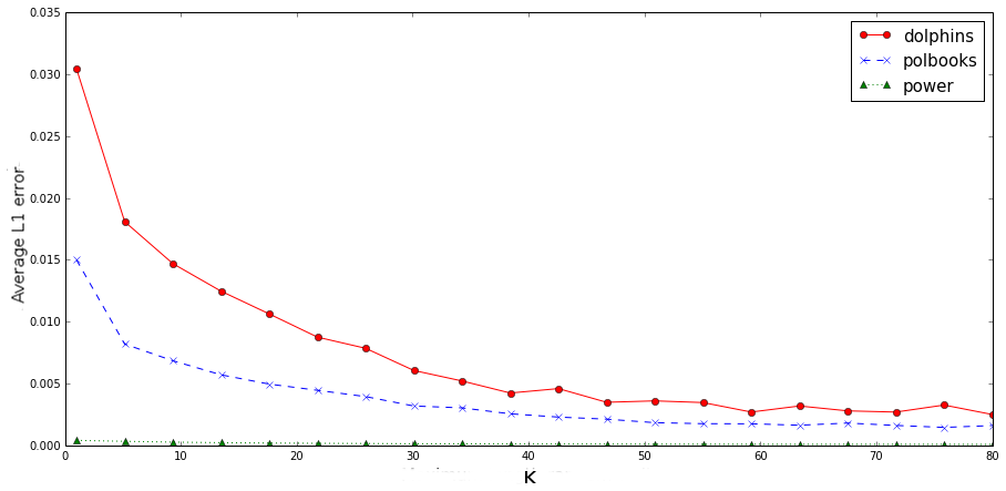
Figure 3: Average error in each component for $\epsilon$-approximate heat kernel pagerank vectors when allowing varying random walk lengths.

Figure 4: Intersersection difference of the ranked lists of vertices computed by exact and $\epsilon$-approximate heat kernel pagerank vectors when allowing varying random walk lengths.

First we discuss the average $L_{1}$ error. The dolphins and the polbooks graphs exihibit properties of both the small world graphs and the preferential attachment graphs of the previous section (Figures 1 and 2). Like the preferential attachment models, there is a significant drop in average $L_{1}$ error after $K=5$, and like the small world model the error continues to drop for larger values of $K$, approaching a minimum error of $\approx 0.003$. The average $L_{1}$ error in the power graph, on the other hand, is small for all values of $K$. We remark that, representing a power grid, the graph has very small average vertex degree, so few random walk steps are enough to approximate the stationary distribution.

As for the intersection difference, we observe a smaller variance in values for the three graphs. Regardless of the size or structure of the graph, the intersection difference drops sharply from $K=1$ to $K=5$. For values larger than $K=10<4\cdot\frac{\log(\epsilon^{-1})}{\log\log(\epsilon^{-1})}$, where $\epsilon=0.1$, the intersection difference decreases only marginally.

The purpose of these experiments was to evaluate how error and differences of ranking change in heat kernel pagerank approximation when varying $K$, the upper bound on number of steps taken in random walks. We found that setting an upper bound for random walk lengths to $K=10<4\cdot\frac{\log(\epsilon^{-1})}{\log\log(\epsilon^{-1})}$ with $\epsilon=0.1$ according to Theorem 3.1 yields approximations which satisfy the prescribed error bounds. This value is independent of the size of the graph and $t$, and depends only on $\epsilon$. Namely, we observed that choosing $K$ this way results in a significant decrease in both average $L_{1}$ error and intersection difference as compared to smaller values of $K$, and only slight decrease in average $L_{1}$ error and intersection difference for larger values of $K$ as demonstrated in Figures 1, 2, 3, and 4. Further, we tested graphs of various size, random graphs generated from various models (see Section 5.1), and graphs from real data representing social networks, copurchasing networks, and topological grids (see Section 5.2). We found this choice of $K$ was optimal for every graph regardless of size or structure. That is, the cutoff for random walk lengths does not depend on the size of the graph.

It is also worth mentioning that the most striking outlier among the subject graphs is the small world graph, or expander graphs. This is due to the fact that the graph consists of a single cluster, which makes local cluster detection ineffective.

6 An Assessment of Cheeger Ratios Obtained with Local Clustering Algorithms

The goal of this section is to analyze the quality of local clusters computed with a sweep over an approximate heat kernel pagerank vector (see Section 4 for details on sweeps). We consider two objectives for analysis.

The first objective is to validate the statement of Theorem 4.3. To do this, we show that the Cheeger ratios of local clusters computed with sweeps over approximate heat kernel pagerank vectors are within the approximation guarantees of Theorem 4.3. We use a slightly modified version of ClusterHKPR to compute these clusters. We call this modified algorithm $\epsilon$HKPR, and it is described in the list below.

The second objective is to compare clusters computed with sweeps over different vectors. Namely, for a given graph and seed vertex, we compare the local clusters computed using the following sweep algorithms:

1. ($\epsilon$HKPR) A sweep over an $\epsilon$-approximate heat kernel pagerank vector is performed. The segment $S$ with volume $\textmd{vol}(S)\leq\textmd{vol}(G)/2$ of minimal Cheeger ratio is output. This is the ClusterHKPR algorithm with the following modification: we allow segments of volume up to $\textmd{vol}(G)/2$ rather than limiting the search to segments of volume $<2\varsigma$, twice the target volume.

2. (HKPR) A sweep over an exact heat kernel pagerank vector is performed. The segment $S$ with volume $\textmd{vol}(S)\leq\textmd{vol}(G)/2$ of minimal Cheeger ratio is output. This algorithm was outlined, but not stated explicitely, in [10].

3. (PR) A sweep over a Personalized PageRank vector (4) is performed. The segment $S$ with volume $\textmd{vol}(S)\leq\textmd{vol}(G)/2$ of minimal Cheeger ratio is output. This is an adaptation of the algorithm PageRank-Nibble[3] with the following modifications: (i) rather than performing a sweep over an approximate PageRank vector, perform a sweep over an exact PageRank vector, and (ii) allow segments only as large as $\textmd{vol}(G)/2$.

We summarize the algorithms and parameters below in Table 6.

Algorithm	Sweep vector	Algorithm parameters	Sweep vector parameters
$\epsilon$HKPR	$\hat{\rho}_{t,u}$	$\phi$, target Cheeger ratio	$t=\phi^{-1}\log(\frac{2\sqrt{\varsigma}}{1-\epsilon}+2\epsilon s)$
		$s$, target cluster size	$u$, seed vertex
		$\varsigma$, target cluster volume	$\epsilon$, approximation parameter
HKPR	$\rho_{t,u}$	$\phi$, target Cheeger ratio	$t=2\phi^{-1}\log s$
		$s$, target cluster size	$u$, seed vertex
PR	$\textsf{pr}_{\alpha,u}$	$\phi$, target Cheeger ratio	$\alpha=\phi^{2}/255\ln(100\sqrt{m})$
			$u$, seed vertex

Table 6: Algorithms used for comparing local clusters.

Each trial will resemble Procedure 1, as stated below.

Procedure 1 Compare Clusters

Let $G$ be a graph and $u$ a seed vertex

Choose parameters $\phi$, $s$, $\varsigma$, $\epsilon$

Let $S_{A}$ be a local cluster computed using the algorithm $\epsilon$HKPR

Let $S_{B}$ be a local cluster computed using the algorithm HKPR

Let $S_{C}$ be a local cluster computed using the algorithm PR

Compare $S_{A},S_{B},S_{C}$.

The following sections describe the experiments in more detail.

6.1 Synthetic graphs

In this section, we use graphs generated with three random graph models: Watts-Strogatz small world, Barabási-Albert preferential attachment, and Holme and Kim’s powerlaw cluster as described in Section 5.1.

6.1.1 Procedure

We perform twenty-five trials of Procedure 1 and take the averages of Cheeger ratios and cluster volumes computed. Specifically, we fix a model and algorithm parameters. Then, generate a random graph according to the model and parameters. For each random graph, pick a random seed vertex with probability proportional to degree. Then, for each seed vertex compute local clusters $S_{A},S_{B},S_{C}$ using the algorithms $\epsilon$HKPR, HKPR, and PR, respectively. We then use the average Cheeger ratio and cluster volume of the $S_{A},S_{B},S_{C}$ for comparison. In Table 7 we summarize the parameters used for each random graph model.

Model	$|V|~{}~{}$	$d$	$p$	$\epsilon$	Target	Target	Target
					Cheeger ratio	cluster size	cluster volume
small world	$100$	$5$	$0.1$	$0.1$	$0.1$	$20$	$100$
	$500$	$5$	$0.1$	$0.1$	$0.1$	$100$	$500$
	$800$	$5$	$0.1$	$0.1$	$0.1$	$100$	$500$
	$1000$	$5$	$0.1$	$0.1$	$0.1$	$100$	$500$
preferential	$100$	$5$	-	$0.1$	$0.1$	$20$	$100$
attachment	$500$	$5$	-	$0.1$	$0.1$	$100$	$500$
	$800$	$5$	-	$0.1$	$0.1$	$100$	$500$
powerlaw	$100$	$5$	$0.1$	$0.1$	$0.1$	$20$	$100$
cluster	$500$	$5$	$0.1$	$0.1$	$0.1$	$100$	$500$
	$800$	$5$	$0.1$	$0.1$	$0.1$	$100$	$500$

Table 7: Algorithm parameters used to compare local clusters.

6.1.2 Discussion

We address the first analytic objective listed in the introduction of this section by discussing the clusters output by $\epsilon$HKPR. Namely, we compare the clusters computed with $\epsilon$HKPR to the guarantees of Theorem 4.3. The results for each graph are given in Table 8. The first three columns indicate the random graph model and algorithm parameters used for each instance. The last two columns demonstrate how the (average) Cheeger ratio of clusters computed by $\epsilon$HKPR compare to the approximation guarantee of Theorem 4.3. Namely, Theorem 4.3 states that the cluster output will have Cheeger ratio $\leq\sqrt{8\phi}$ with high probability. In every case the Cheeger ratio is well within the approximation bounds.

Synthetic graphs
Model   $|V|$ $\phi$, Target Cheeger ratio output by      $\sqrt{8\phi}$ Cheeger ratio $\epsilon$HKPR small world $100$ $0.1$ $0.173557$ $0.894427$ $500$ $0.1$ $0.47316$ $0.894427$ $800$ $0.1$ $0.510597$ $0.894427$ $1000$ $0.1$ $0.519399$ $0.894427$ preferential $100$ $0.1$ $0.523929$ $0.894427$ attachment $500$ $0.1$ $0.503542$ $0.894427$ $800$ $0.1$ $0.491046$ $0.894427$ powerlaw $100$ $0.1$ $0.517521$ $0.894427$ cluster $500$ $0.1$ $0.500312$ $0.894427$ $800$ $0.1$ $0.494145$ $0.894427$

Table 8: Cheeger ratios of cluster output by $\epsilon$HKPR.

The second objective is to compare clusters computed with the three different local clustering algorithms $\epsilon$HKPR, HKPR, and PR. Table 9 is a collection of cluster statistics for the trials. For each graph instance we list the average Cheeger ratio and cluster volume of local clusters computed using the PR, HKPR, and $\epsilon$HKPR algorithms, respectively.

Synthetic graphs
Model $|V|$ PR HKPR $\epsilon$HKPR small world 100 $0.235159$ $0.087723$ $0.173557$ (volume = $52.52$) (volume = $171.28$) (volume = $142$) 500 $0.244261$ $0.062263$ $0.47316$ (volume = $190.16$) (volume = $943.68$) (volume = $206.64$) 800 $0.246564$ $0.064599$ $0.510597$ (volume = $162.68$) (volume = $1413.6$) (volume = $209.6$) 1000 $0.245612$ $0.064716$ $0.519399$ (volume = $584.56$) (volume = $1907.4$) (volume = $225.2$) preferential 100 $0.430071$ $0.512819$ $0.523929$ attachment (volume = $471.2$) (volume = $467.16$) (volume = $468.16$) 500 $0.508305$ $0.51018$ $0.503542$ (volume = $2461.96$) (volume = $2459.4$) (volume = $2463.28$) 800 $0.491046$ $0.496369$ $0.491046$ (volume = $3964.17$) (volume = $3971.17$) (volume = $3951.83$) powerlaw 100 $0.426828$ $0.505277$ $0.517521$ cluster (volume = $463.4$) (volume = $465.44$) (volume = $464.88$) 500 $0.487341$ $0.507328$ $0.500312$ (volume = $2447.12$) (volume = $2460.44$) (volume = $2446.28$) 800 $0.522281$ $0.513365$ $0.494145$ (volume = $3947$) (volume = $3966$) (volume = $3947$)

Table 9: Cheeger ratios of clusters output by different local clustering algorithms on synthetic data.

We remark that for each graph there is little variation in Cheeger ratio and volume of clusters computed by the three different algorithms. We also note that there is no obvious trend as graphs get larger. The small world graphs demonstrate the greatest variation in cluster quality. However, as mentioned in Section 5, expander graphs, such as small world graphs, consist of one large cluster.

It is worth noting that in some trials the output volume is significantly greater than twice the target volume. While this may seem like a contradiction, it is a consequence of our implementation. During a sweep one may choose to output a cluster of minimal Cheeger ratio, or one that satisfies volume constraints, or both. We are interested in comparing Cheeger ratios and so allow the sweep to continue checking clusters that are well beyond twice the target volume.

6.2 Real graphs

For these trials we use graphs generated from real data summarized in Section 5.2.

6.2.1 Procedure

We compare clusters computed by each of the three algorithms as outlined in Procedure 1. In these trials we fix the seed vertex to be a member of a cluster with good Cheeger ratio. Using this seed vertex, we compare the clusters computed using the $\epsilon$HKPR, HKPR, PR algorithms.

For each trial we use the parameters listed in Table 10. We note that in each case the target cluster volume is computed to be roughly the target cluster size times the average vertex degree, and here we use $\epsilon=0.1$.

Network	$|V|$	$|E|$	Average	$\epsilon$	Target	Target	Target
			degree		Cheeger ratio	cluster size	cluster volume
dolphins	$62$	$159$	$5$	$0.1$	$0.08$	$20$	$100$
polbooks	$105$	$441$	$8.8$	$0.1$	$0.05$	$30$	$270$
power	$4941$	$6594$	$2.7$	$0.1$	$0.05$	$200$	$600$
facebook	$4039$	$88234$	$43.7$	$0.1$	$0.05$	$200$	$2800$
enron	$36692$	$183831$	$10$	$0.1$	$0.05$	$100$	$1000$

Table 10: Graph and algorithm parameters used to compare local clusters.

6.2.2 Discussion

Table 11 lists ratios output by $\epsilon$HKPR compared with the approximation guarantees of Theorem 4.3. In each case, the Cheeger ratios are well within the approximation bounds of Theorem 4.3.

Real graphs
Network $\phi$, Target Cheeger ratio output by      $\sqrt{8\phi}$ Cheeger ratio $\epsilon$HKPR dolphins $0.08$ $0.083333$ $0.8$ polbooks $0.05$ $0.052133$ $0.632456$ power $0.05$ $0.346667$ $0.632456$ facebook $0.05$ $0.056939$ $0.632456$ enron $0.05$ $0.036602$ $0.632456$

Table 11: Cheeger ratios of cluster output ClusterHKPR.

The complete numerical data obtained from the set of the trials are given in Table 12. For each graph we list the Cheeger ratio, cluster volume, and additionally the cluster size of local clusters computed using each of the algorithms PR, HKPR, and $\epsilon$HKPR, respectively.

Real graphs
Network PR HKPR $\epsilon$HKPR dolphins $0.226415$ $0.163636$ $0.083333$ (volume = $106$) (volume = $110$) (volume = $96$) (size = $23$) (size = $24$) (size = $20$) polbooks $0.079518$ $0.245657$ $0.052133$ (volume = $415$) (volume = $403$) (volume = $422$) (size = $48$) (size = $49$) (size = $50$) power $0.375$ $0.002764$ $0.346668$ (volume = $16$) (volume = $4342$) (volume = $300$) (size = $6$) (size = $1564$) (size = $85$) facebook $0.418993$ $0.001277$ $0.056939$ (volume = $88140$) (volume = $67326$) (volume = $35266$) (size = $3063$) (size = $1094$) (size = $258$) enron $0.48797$ - $0.036602$ (volume = $183612$) - (volume = $3579$)

Table 12: Cheeger ratios of cluster output by different local clustering algorithms.

For each graph, the local cluster computed using $\epsilon$HKPR has smaller Cheeger ratio than the local cluster computed using PR. For the power graph, we observe that the cluster of minimal Cheeger ratio was computed using the HKPR algorithm, but it is nearly a third the size of the entire network. The algorithms $\epsilon$HKPR and PR, on the other hand, each return smaller clusters. We remark that for real graphs, the clusters computed using sweeps over different vectors have more variation than for random graphs.

At this point we remark about our choice of parameters for the trials. At this point the sensitivity of the algorithm to the choice of $\epsilon,\phi,s,$ and $\varsigma$ has not been fully explored. In particular, it is worth studying the effect of $\phi$ on the output cluster in future work.

To conclude, we include visualizations of clusters computed in the facebook ego-network to illustrate the differences in local cluster detection. Figure 5 colors the vertices in a local cluster computed using the $\epsilon$HKPR algorithm, as described in Table 12. Figure 6 colors the vertices in a local cluster compted using the PR algorithm.

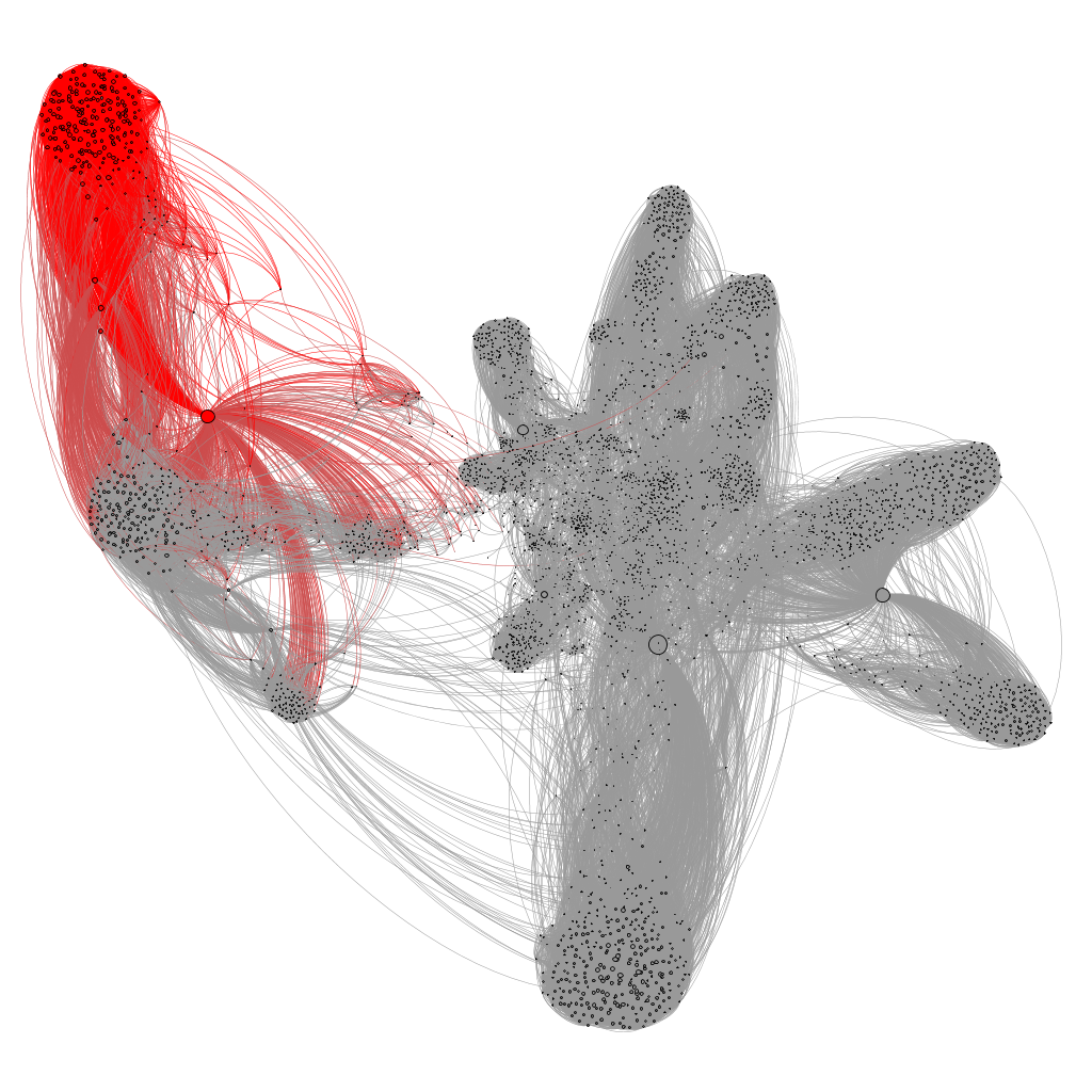
Figure 5: Local cluster in facebook ego network computed using the $\epsilon$HKPR algorithm.

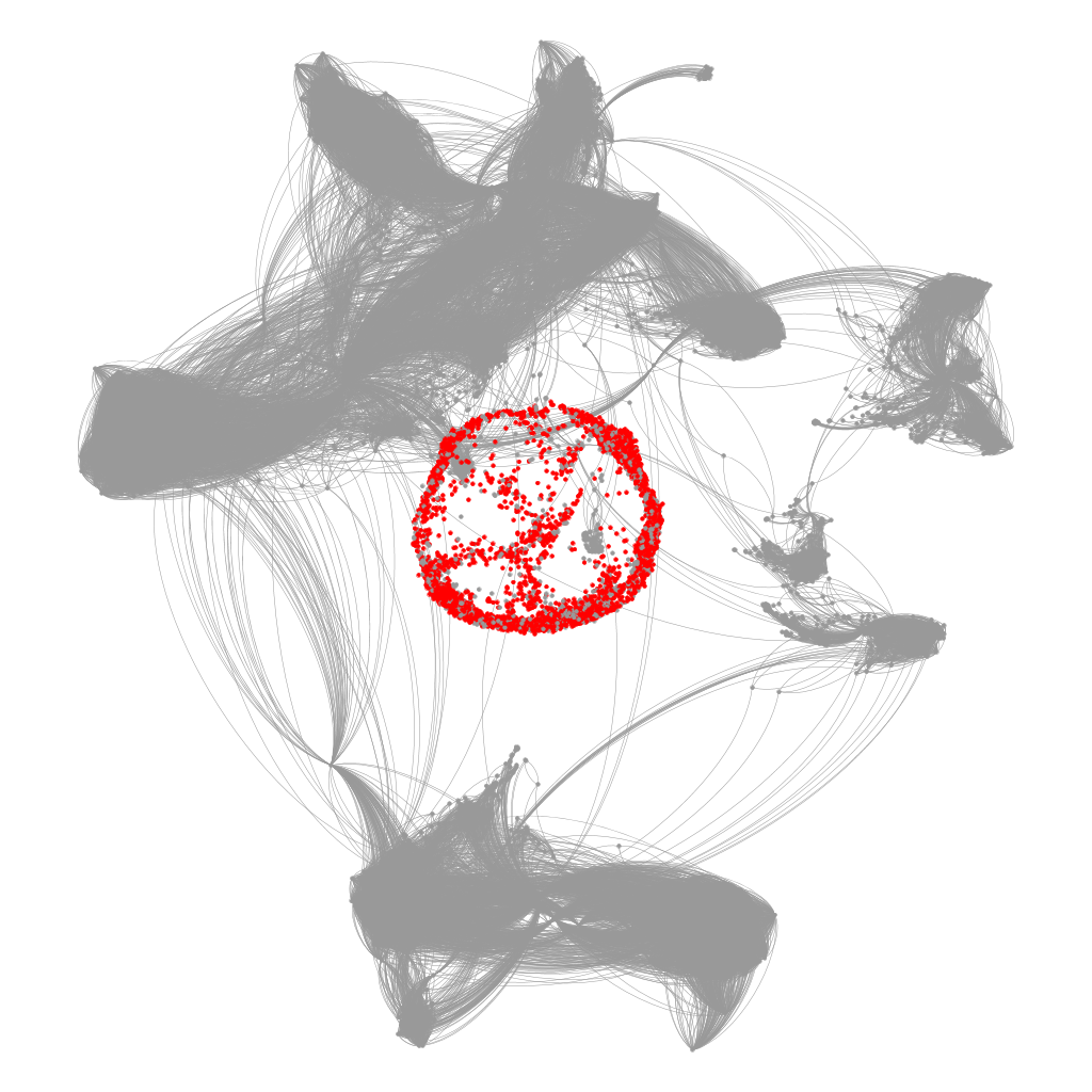
Figure 6: Local cluster in facebook ego network computed using the PR algorithm.

The numerical data of the last two sections validate the effectiveness and efficiency of local cluster detection using sweeps over $\epsilon$-approximate heat kernel pagerank. The experiments of Section 5 demonstrate that sampling a number of random walks of at most $K$ steps yield a ranking of vertices within the error bounds of Theorem 3.1. This ranking in turn is used to compute a local cluster. What is more, this value $K$ does not depend on parameters other than $\epsilon$. Specifically, it does not depend on the size of the graph or the desired cluster volume, size, or Cheeger ratio. Finally, the data of Section 6 validate the statements of Theorem 4.3. That is, perfoming a sweep over an approximate heat kernel pagerank vector detects clusters of Cheeger ratio at most $\sqrt{8\phi}$ for a desired Cheeger ratio $\phi$. The total cost of computing this cluster is $O\big{(}\frac{\log(\epsilon^{-1})\log n}{\epsilon^{3}\log\log(\epsilon^{-1})}\big{)}$, sublinear in the size of the graph.

References

- [1] Noga Alon and Vitali D. Milman, , isoperimetric inequalities for graphs, and superconductors, Journal of Combinatorial Theory, Series B 38 (1985), no. 1, 73–88.
- [2] Reid Andersen and Fan Chung, Detecting sharp drops in pagerank and a simplified local partitioning algorithm, Proceedings of Theory and Applications of Models of Computation, Springer, 2007, pp. 1–12.
- [3] Reid Andersen, Fan Chung, and Kevin Lang, Local graph partitioning using pagerank vectors, IEEE 47th Annual Symposium on Foundations of Computer Science, IEEE, 2006, pp. 475–486.
- [4] Reid Andersen and Yuval Peres, Finding sparse cuts locally using evolving sets, Proceedings of the 41st Annual Symposium on Theory of Computing, ACM, 2009, pp. 235–244.
- [5] Albert-László Barabási and Réka Albert, Emergence of scaling in random networks, Science 286 (1999), no. 5439, 509–512.
- [6] Michele Benzi and Christine Klymko, Total communicability as a centrality measure, Journal of Complex Networks 1 (2013), no. 2, 124–149.
- [7] Christian Borgs, Michael Brautbar, Jennifer T. Chayes, and Shang-Hua Teng, A sublinear time algorithm for pagerank computations, WAW, 2012, pp. 41–53.
- [8] Pak K. Chan, Martine D.F. Schlag, and Jason Y. Zien, Spectral k-way ratio-cut partitioning and clustering, IEEE Transactions on Computer-Aided Design of Integrated Circuits and Systems 13 (1994), no. 9, 1088–1096.
- [9] Fan Chung, The heat kernel as the pagerank of a graph, Proceedings of the National Academy of Sciences 104 (2007), no. 50, 19735–19740.
- [10] , A local graph partitioning algorithm using heat kernel pagerank, Internet Mathematics 6 (2009), no. 3, 315–330.
- [11] Fan Chung and Olivia Simpson, Solving linear systems with boundary conditions using heat kernel pagerank, Workshop on Algorithms and Models for the Web Graph, 2013, pp. 203 – 219.
- [12] , Computing heat kernel pagerank and a local clustering algorithm, Combinatorial Algorithms: 25th International Workshop, IWOCA 2014, Duluth, MN, USA, October 15-17, 2014, Revised Selected Papers, Springer, 2014, pp. 110–121.
- [13] , Solving local linear systems with boundary conditions using heat kernel pagrank, Internet Mathematics 11 (2015), no. 4-5, 449–471.
- [14] William E. Donath and Alan J. Hoffman, Algorithms for partitioning of graphs and computer logic based on eigenvectors of connection matrices, IBM Technical Disclosure Bulletin 15 (1972), no. 3, 938–944.
- [15] Ronald Fagin, Ravi Kumar, and D. Sivakumar, Comparing top lists, SIAM Journal on Discrete Mathematics 17 (2003), no. 1, 134–160.
- [16] Shayan Oveis Gharan and Luca Trevisan, Approximating the expansion profile and almost optimal local graph clustering, IEEE 53rd Annual Symposium on Foundations of Computer Science, IEEE, 2012, pp. 187–196.
- [17] Aric A. Hagberg, Daniel A. Schult, and Pieter J. Swart, Exploring network structure, synamics, and function using NetworkX, Proceedings of the 7th Python in Science Conference (SciPy2008) (Pasadena, CA USA), August 2008, pp. 11–15.
- [18] Taher H Haveliwala, Topic-sensitive pagerank, Proceedings of the 11th international conference on World Wide Web, ACM, 2002, pp. 517–526.
- [19] Petter Holme and Beom Jun Kim, Growing scale-free networks with tunable clustering, Physical Review E 65 (2002), no. 2, 026107.
- [20] Ravi Kannan, Santosh Vempala, and Adrian Vetta, On clusterings: Good, bad and spectral, Journal of the ACM (JACM) 51 (2004), no. 3, 497–515.
- [21] Bryan Klimt and Yiming Yang, Introducing the enron corpus., CEAS, 2004.
- [22] Kyle Kloster and David F. Gleich, A nearly-sublinear method for approximating a column of the matrix exponential for matrices from large, sparse networks, Algorithms and Models for the Web Graph, 2013, pp. 68–79.
- [23] Valdis Krebs, New political patterns, http://www.orgnet.com/divided, 2008.
- [24] Jure Leskovec and Andrej Krevl, SNAP Datasets: Stanford large network dataset collection, http://snap.stanford.edu/data, June 2014.
- [25] Jure Leskovec, Kevin J. Lang, Anirban Dasgupta, and Michael W. Mahoney, Statistical properties of community structure in large social and information networks, Proceedings of the 17th International Conference on World Wide Web, ACM, 2008, pp. 695–704.
- [26] Jure Leskovec and Julian J Mcauley, Learning to discover social circles in ego networks, Advances in Neural Information Processing Systems, 2012, pp. 539–547.
- [27] Chung-Shou Liao, Kanghao Lu, Michael Baym, Rohit Singh, and Bonnie Berger, Isorankn: Spectral methods for global alignment of multiple protein networks, Bioinformatics 25 (2009), no. 12, i253–i258.
- [28] Frank Lin and William W. Cohen, Power iteration clustering, Proceedings of the 27th International Conference on Machine Learning(ICML10), 2010, pp. 655–662.
- [29] , A very fast method for clustering big text datasets, Proceedings of the 19th European Conference on Artificial Intelligence, 2010, pp. 303–308.
- [30] László Lovász and Miklós Simonovits, The mixing rate of markov chains, an isoperimetric inequality, and computing the volume, Proceedings of the 31st Annual Symposium on Foundations of Computer Science, IEEE, 1990, pp. 346–354.
- [31] , Random walks in a convex body and an improved volume algorithm, Random Structures & Algorithms 4 (1993), no. 4, 359–412.
- [32] D. Lusseau, K. Schneider, O.J Boisseau, P. Haase, E. Slooten, and S.M. Dawson, The bottlenose dolphin community of doubtful sound features a large proportion of long-lasting associations, Behavioral Ecology and Sociobioloy 54 (2003), 396–405.
- [33] Mark Newman, Network data, http://www-personal.umich.edu/~mejn/netdata/, 2013.
- [34] Andrew Y Ng, Michael I Jordan, Yair Weiss, et al., On spectral clustering: Analysis and an algorithm, Advances in neural information processing systems 2 (2002), 849–856.
- [35] Lorenzo Orecchia, Sushant Sachdeva, and Nisheeth K. Vishnoi, Approximating the exponential, the lanczos method and an (m)-time spectral algorithm for balanced separator, Proceedings of the 44th Symposium on Theory of Computing, ACM, 2012, pp. 1141–1160.
- [36] Sushant Sachdeva and Nisheeth K. Vishnoi, Matrix inversion is as easy as exponentiation, arXiv preprint arXiv:1305.0526 (2013).
- [37] Jianbo Shi and Jitendra Malik, Normalized cuts and image segmentation, IEEE Transaction on Pattern Analysis and Machine Intelligence 22 (2000), no. 8, 888–905.
- [38] Daniel A. Spielman and Shang-Hua Teng, Nearly-linear time algorithms for graph partitioning, graph sparsification, and solving linear systems, Proceedings of the thirty-sixth annual ACM symposium on Theory of Computing, ACM, 2004, pp. 81–90.
- [39] , A local clustering algorithm for massive graphs and its application to nearly-linear time graph partitioning, CoRR abs/0809.3232 (2008).
- [40] Duncan J. Watts and Steven H. Strogatz, Collective dynamics of ‘small-world’ networks, Nature 393 (1998), no. 6684, 440–442.
- [41] , Collective dynamics of ‘small-world’ networks, Nature 393 (1998), no. 6684, 440–442.