Scalable quantum information transfer between nitrogen-vacancy-center ensembles

Abstract

We propose an architecture for realizing quantum information transfer (QIT). In this architecture, a LC circuit is used to induce the necessary interaction between flux qubits, each magnetically coupling to a nitrogen-vacancy center ensemble (NVCE). We explicitly show that for resonant interaction and large detuning cases, high-fidelity QIT between two spatially-separated NVCEs can be implemented. Our proposal can be extended to achieve QIT between any two selected NVCEs in a large hybrid system by adjusting system parameters, which is important in large scale quantum information processing.

I introduction

Quantum information transfer (QIT) has many applications in communication science a0 . There exist physical systems for realizing QIT, such as, cavity quantum electrodynamics (QED) a01 ; a02 ; a021 ; a022 , linear optics devices a03 , and superconducting qubits a04 ; a05 ; a06 ; a07 ; a08 , etc. In addition, a nitrogen-vacancy center in diamond has been recently considered as one of the most promising candidates for quantum information processing, due to its relatively long coherence time and the possibility of coherent manipulation at room temperature b . For instances, the electron spin relaxation time $T_{1}=6$ms c and isotopically pure diamond sample dephasing time $T_{2}=2$ms d have been reported, coherent oscillations in a single electron spin have been observed d1 , and coherent time of a nitrogen-vacancy center has been improved very much in the recent years and could reach $1$ second d11 . On the other hand, hybrid solid-state devices have attracted tremendous attentions (see a and references therein). Theoretically, the physical systems, composed of spin ensembles and superconducting qubits fabricated in a TLR (transmission line resonator), have been proposed a1 ; a2 ; a3 ; a33 . Experimentally, a quantum circuit consisting of a superconducting qubit and a nitrogen-vacancy center ensemble (NVCE) has been implemented in Ref. a4 ; and a quantum SWAP gate has been realized in this circuit, by employing the strong coupling between a superconducting qubit and a NVCE a4 . In addition, Marcos et al. a5 have proposed a hybrid system, in which the direct coupling between a superconducting flux qubit and a NVCE is much stronger than that between a NVCE and a TLR. For the work on the coupling between a NVCE and a TLR, see Refs. d3 ; d4 . Experimentally, the strong coupling between a superconducting flux qubit and a NVCE has been demonstrated a6 . Moreover, by using the strong coupling, the QIT between a flux qubit and a NVCE has been performed in experiment a7 . Then, the strong coupling between a NVCE and a TLR via a flux qubit used as a data bus was proposed in Ref. a8 . These results provide a platform for using NVCEs as quantum memories, which are essential in quantum information processing.

Motivated by the recent works on the coupling between LC circuits and flux qubits a9 ; a10 ; a11 ; a12 , and the strong coupling hybrid solid quantum system a5 ; a6 ; a7 ; a8 , as well as the QIT with the solid quantum system a80 ; a81 ; a82 , we will propose an architecture for scalable QIT among NVCEs. In this architecture, a LC circuit is used to induce the necessary interaction between flux qubits, each magnetically coupling to a NVCE. We explicitly show that for resonant interaction and large detuning cases, high-fidelity QIT between the two spatially-separated NVCEs can be implemented by solving Schrödinger equations. Moreover, this architecture can be extended to scale up multiple flux qubits and NVCEs by using a single LC circuit, and the QIT between any two selected NVCEs can be achieved in this large hybrid system. To the best of our knowledge, how to realize QIT between NVCEs in this architecture has not been proposed yet. Note that, Refs. a13 ; a14 reported the QIT between two ensembles which are trapped in spatially separated cavities, respectively. But, the fidelity of the QIT was not calculated and the dissipation of the system was not considered in Refs. a13 ; a14 .

II Model

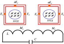
Figure 1: (Color online) Quantum information transfer circuit. Two flux qubits are coupled to a LC circuit by their mutual inductances $M_{j}$ (j=1,2). Each flux qubit consists of three Josephson junctions, i.e., two large junctions with the same coupling energy $E_{J}$ and a small junction with the coupling energy $\alpha E_{J}~{}(0.5<\alpha<1)$. The separation between the two qubits is assumed to be much larger than the linear dimension of each qubit, such that the direct interaction between the two flux qubits is negligible. Here, the NVCEs play a role of memory units, which are used to store quantum information for a long time.

We propose a QIT hybrid circuit, as shown in Fig. (1), which consists of a LC circuit acting as a data bus to induce coupling between two flux qubits. Each flux qubit couples to a NVCE by a magnetic field. Each NVCE is an information memory unit. The electronic ground state of a single nitrogen-vacancy center (NVC) has a spin $\mathbb{S}=1$, with the levels $m_{s}=0$ and $m_{s}=\pm 1$ separated by zero-field splitting $D$. For a NVC, the Hamiltonian can be described by (assuming $\hbar=1$) e0 ; e

$$H_{NVC}=D\mathbb{S}^{2}_{z}+E(\mathbb{S}^{2}_{x}-\mathbb{S}^{2}_{y})+g_{e}\mu_{B}\vec{B}\cdot\vec{\mathbb{S}},$$ (1)

where zero field splitting $D=2.88$ GHz, $\vec{\mathbb{S}}=\{\mathbb{S}_{x},\mathbb{S}_{y},\mathbb{S}_{z}\}$ is a usual Pauli spin-1 operator, $E$ is the strain-induced splitting coefficient, $B$ is the applied magnetic field, $g_{e}$ is the Lande factor, and $\mu_{B}$ is the Bohr magneton. When the static magnetic field $\vec{B}$ is applied along the crystalline axis of the diamond, the degeneracy of levels $|m_{s}=\pm 1\rangle$ can be removed. The quantum information is encoded in sublevels $|m_{s}=0\rangle\equiv|0\rangle$ and $|m_{s}=-1\rangle\equiv|1\rangle$ serving as two logic states of a qubit. For a NVCE with NVCs ($1,2,\ldots N$), the ground state is defined as $|g\rangle=|0_{1}\cdots 0_{k}\cdots 0_{N}\rangle$ while the excited state is defined as $|e\rangle=S^{+}|g\rangle=(1/\sqrt{N})\sum_{k=1}^{N}|0_{1}\cdots 1_{k}\cdots 0_{N}\rangle$ with operator $S^{+}=(S^{-})^{{\dagger}}=(1/\sqrt{N})\sum_{k}^{N}|1\rangle_{k}\langle 0|$, where the subscript k represents the k-th NVC. Thus, the Hamiltonian of a NVCE is written as a3 $H_{NVCE}=\frac{1}{2}\Omega S_{z}$, where $\Omega=D-g_{e}\mu_{B}B_{z}$ is the energy gap between the ground state $|g\rangle$ and the excited state $|e\rangle$, with the operator $S_{z}=|e\rangle\langle e|-|g\rangle\langle g|$.

The Hamiltonian of a flux qubit is described as a two-level system f0 ; f

$$H_{q}=\frac{1}{2}(\varepsilon\sigma_{z}+\Delta\sigma_{x}),$$ (2)

where $\varepsilon(\Phi)=2I_{p}[\Phi-(1/2+n)\Phi_{0}]$ is the energy spacing of the two classical current states, $I_{p}$ is persistent current of the flux qubit, $\Phi_{0}=h/2e$ is the magnetic-flux quantum, $\Phi$ is the external magnetic flux applied to the qubit loop, $\Delta$ is the energy gap between the two energy levels of the qubit at the degeneracy point, and Pauli matrices $\sigma_{z}=|b\rangle\langle b|-|a\rangle\langle a|$ and $\sigma_{x}=|b\rangle\langle a|+|a\rangle\langle b|$ are defined in terms of the classical current, with $|a\rangle=|\circlearrowright\rangle$ and $|b\rangle=|\circlearrowleft\rangle$ denoting the states with clockwise and counterclockwise currents in the qubit loop. In terms of the eigenbasis of the flux qubit, the Hamiltonian (2) can be rewritten as $H_{q}=\frac{1}{2}\omega_{q}\sigma_{z}$, with $\hbar\omega_{q}=\sqrt{\varepsilon^{2}+\Delta^{2}}$ being the energy level separation of the flux qubit.

As long as the distance between the two flux qubits is large, the direct interaction between the two flux qubits is negligible. For a system in Fig. 1, the total Hamiltonian is given by

$$H = \omega a^{{\dagger}}a+\sum_{j=1}^{2}[\frac{1}{2}\omega^{j}_{q}\sigma^{j}_{z}+g_{j}(a\sigma_{j}^{+}+a^{{\dagger}}\sigma_{j}^{-})$$ (3)

$$+\frac{1}{2}\Omega_{j}S^{j}_{z}+J_{j}(S_{j}^{+}\sigma_{j}^{-}+S_{j}^{-}\sigma_{j}^{+})],$$

where the first term is the free Hamiltonian of the LC circuit with the resonance frequency $\omega=1/\sqrt{LC}$ and the plasmon annihilation (creation) operator $a~{}(a^{{\dagger}})$ a11 , the third term represents the interaction between the LC circuit and the flux qubits with the coupling constant $g_{j}=M_{j}I_{p}\sqrt{\omega/2L}$ a11 and the operator $\sigma^{{\dagger}}_{j}=(\sigma^{-}_{j})^{{\dagger}}=|1\rangle_{j}\langle 0|$, the last term indicates the coupling between NVCEs and flux qubits with the coupling strength $J_{j}$ a5 .

III Quantum information transfer

In this section, we discuss how to realize QIT between spatially-separated two NVCEs for both resonant interaction and large detuning cases. By solving Schrödinger equations, we find that high-fidelity QIT can be implemented at some moment, as shown below.

For simplicity, we use NE to represent NVCE in each equation below, but still use NVCE in the word text.

III.1 Resonant interaction case

In the interaction picture, the Hamiltonian of the total system for the resonant interaction case (i.e. $\omega=\omega_{q}^{j}=\Omega_{j}$) can be written as follows

$$H_{I}=\sum_{j=1}^{2}[g_{j}(a\sigma_{j}^{+}+a^{{\dagger}}\sigma_{j}^{-})+J_{j}(S_{j}^{+}\sigma_{j}^{-}+S_{j}^{-}\sigma_{j}^{+})].$$ (4)

The QIT from the left NVCE (i.e., $NE_{1}$) to the right one (i.e., $NE_{2}$) is described by the formula $(\alpha|g\rangle+\beta|e\rangle)_{NE_{1}}|0\rangle_{1}|0\rangle_{2}|0\rangle_{L}|g\rangle_{NE_{2}}\rightarrow|g\rangle_{NE_{1}}|0\rangle_{1}|0\rangle_{2}|0\rangle_{L}(\alpha|g\rangle+\beta|e\rangle)_{NE_{2}}$, where the subscripts $1,~{}2$, and $L$ represent the left flux qubit, the right flux qubit, and LC circuit, respectively; $\alpha$ and $\beta$ are the normalized complex numbers. When the initial state of the system is $|\Psi(0)\rangle=|e\rangle_{NE_{1}}|0\rangle_{1}|0\rangle_{2}|0\rangle_{L}|g\rangle_{NE_{2}}$, the system state evolves in the subspace $\{|\varphi_{1}\rangle,|\varphi_{2}\rangle,|\varphi_{3}\rangle,|\varphi_{4}\rangle,|\varphi_{5}\rangle\}$ with

$$|\varphi_{1}\rangle =|e\rangle_{NE_{1}}|0\rangle_{1}|0\rangle_{2}|0\rangle_{L}|g\rangle_{NE_{2}},$$ (5a)

$$|\varphi_{2}\rangle =|g\rangle_{NE_{1}}|1\rangle_{1}|0\rangle_{2}|0\rangle_{L}|g\rangle_{NE_{2}},$$ (5b)

$$|\varphi_{3}\rangle =|g\rangle_{NE_{1}}|0\rangle_{1}|1\rangle_{2}|0\rangle_{L}|g\rangle_{NE_{2}},$$ (5c)

$$|\varphi_{4}\rangle =|g\rangle_{NE_{1}}|0\rangle_{1}|0\rangle_{2}|1\rangle_{L}|g\rangle_{NE_{2}},$$ (5d)

$$|\varphi_{5}\rangle =|g\rangle_{NE_{1}}|0\rangle_{1}|0\rangle_{2}|0\rangle_{L}|e\rangle_{NE_{2}},$$ (5e)

where $|g\rangle_{NE_{j}}$ and $|e\rangle_{NE_{j}}~{}(j=1,2)$ are, respectively, the ground state and the symmetric Dicke excitation state of the j-th NVCE, $|0\rangle_{j}$ ($|1\rangle_{j}$) is the ground (excited) state of the j-th flux qubit; $|0\rangle_{L}$ ($|1\rangle_{L}$) is the ground (single-excited) state of the LC circuit. At any instant, the quantum state of the system is described by

$$|\Psi(t)\rangle=\sum_{i=1}^{5}C_{i}(t)|\varphi_{i}\rangle,$$ (6)

where the normalized coefficients satisfy $\sum_{i=1}^{5}|C_{i}(t)|^{2}=1$. Suppose the two flux qubits equally couple to the LC circuit ($g_{1}=g_{2}=g$) and equally couple with their NVCEs ($J_{1}=J_{2}=J$). In this case, for the initial conditions $C_{1}(0)=1$ and $C_{2}(0)=C_{3}(0)=C_{4}(0)=C_{5}(0)=0$, we can easily get the expression of the time-dependent coefficients,

$$C_{1}(t) =\frac{g^{2}}{J^{2}+2g^{2}}+\frac{1}{2}\cos Jt+\frac{J^{2}}{2(J^{2}+2g^{2})}\cos\sqrt{J^{2}+2g^{2}}t,$$ (7a)

$$C_{2}(t) =-i\frac{1}{2}\sin Jt-i\frac{J}{2\sqrt{J^{2}+2g^{2}}}\sin\sqrt{J^{2}+2g^{2}}t,$$ (7b)

$$C_{3}(t) =i\frac{1}{2}\sin Jt-i\frac{J}{2\sqrt{J^{2}+2g^{2}}}\sin\sqrt{J^{2}+2g^{2}}t,$$ (7c)

$$C_{4}(t) =-\frac{Jg}{J^{2}+2g^{2}}+\frac{Jg}{J^{2}+2g^{2}}\cos\sqrt{J^{2}+2g^{2}}t,$$ (7d)

$$C_{5}(t) =\frac{g^{2}}{J^{2}+2g^{2}}-\frac{1}{2}\cos Jt+\frac{J^{2}}{2(J^{2}+2g^{2})}\cos\sqrt{J^{2}+2g^{2}}t.$$ (7e)

The quantum state $|g\rangle_{NE_{1}}|0\rangle_{c1}|0\rangle_{c2}|0\rangle_{L}|g\rangle_{NE_{2}}$ remains unchanged under the Hamiltonian (4). Thus, when the quantum state $|\Psi(t)\rangle$ collapses into $|\varphi_{5}\rangle$, the quantum information is transferred from the left NVCE (i.e., $NE_{1}$) to the right one (i.e., $NE_{2}$). Hence, the populations of quantum states $|\varphi_{1}\rangle$ and $|\varphi_{5}\rangle$ are important measure for the QIT. Our proposal includes two coupling mechanisms: the magnetical coupling $J$ between the flux qubits and the NVCEs, the mutual-inductance coupling $g$ between the flux qubits and the LC circuit. Next, according to the relation between coupling strengths $g$ and $J$, we will analyze the populations of quantum states $|\varphi_{1}\rangle$ and $|\varphi_{5}\rangle$.

Case (i) (the case for the equilibrium coupling $g=J$): the coefficients of quantum state $|\varphi_{1}\rangle$ and $|\varphi_{5}\rangle$ can be written as $C_{1}(t)=1/3+1/2\cos Jt+1/6\cos\sqrt{3}Jt$ and $C_{5}(t)=1/3-1/2\cos Jt+1/6\cos\sqrt{3}Jt$, respectively. In Fig. 2(a), we plot the population change with $Jt$. Obviously, $|C_{5}(t)|^{2}$ can reach the maximum at some moment. This means that QIT between spatially-separated two NVCEs can be perfectly realized.

Case (ii) (the case for the strong magnetic coupling $J\gg g$): if $J\gg g$, $C_{5}(t)$ tends to zero. This result shows that the QIT can not be realized in our system. We plot $|C_{1}(t)|^{2}$ and $|C_{5}(t)|^{2}$ for a coupling strength $J=10g$ in Fig. 2(b), which shows that the QIT between spatially-separated two NVCEs can be realized, but it takes a longer time.

Case (iii) (the case for the strong mutual inductance coupling $J\ll g$): if $J\ll g$, the expressions of $C_{1}(t)$ and $C_{5}(t)$ are reduced to $C_{1}(t)=1/2+1/2\cos Jt$ and $C_{5}(t)=1/2-1/2\cos Jt$, respectively. When $Jt=(2k+1)\pi~{}(k=0,1,2\ldots)$, one has $C_{1}(t)=0$, but $C_{5}(t)=1$, which means that the information has been transferred from the left NVCE to the right one. We have plotted Fig. 2(c) to show how $|C_{1}(t)|^{2}$ and $|C_{5}(t)|^{2}$ change with time $t$ for a coupling strength $J=0.1g$. Fig. 2(c) shows that the QIT between spatially-separated two NVCEs can be implemented.

The recent experiments have reported that the effective coupling strength between a flux qubit and a NVCE (containing $N\sim 3.1\times 10^{7}$ NVCs) can reach $J\sim 70$MHz a6 , and the coupling strength between a flux qubit and a LC circuit can reach $g=220$MHz a9 . Hence, the condition $J\ll g$ for Case (iii) can be well satisfied.

However, in real physical systems the coupling strengths between flux qubits and LC circuit (or NVCEs) are not the same. The expressions of the time-dependent coefficients given in Eqs. (7) become rather long and complicated for the unbalanced coupling case. Here, we only numerically simulate the population change of quantum states with time, as shown in Fig. 3. It can be seen from Fig. 3 that the perfect QIT between spatially-separated two NVCEs can also be realized except for the unbalanced strong magnetic coupling case.

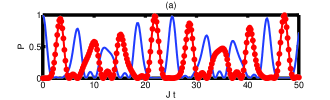
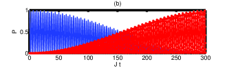
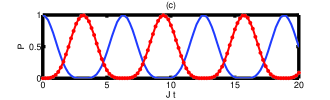
Figure 2: (Color online) Solid-blue lines represent the population $|C_{1}|^{2}$ of the state $|\varphi_{1}\rangle$, while solid-dot-red lines indicate the population $|C_{5}|^{2}$ of the state $|\varphi_{5}\rangle$, (a) the equilibrium coupling $J=g$, (b) the strong magnetic coupling $J=10g$, (c) the strong mutual inductance coupling $J=0.1g$.

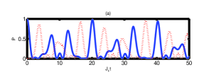
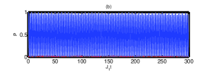
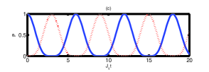
Figure 3: (Color online) Solid-blue lines represent the population $|C_{1}|^{2}$ of the state $|\varphi_{1}\rangle$, while dash lines indicate the population $|C_{5}|^{2}$ of the state $|\varphi_{5}\rangle$, (a) the unbalanced equilibrium coupling $g_{1}=0.9J_{1},~{}g_{2}=0.9J_{2},~{}J_{2}=0.9J_{1}$, (b) the unbalanced strong magnetic coupling $J_{1}=10g_{1},~{}J_{2}=10g_{2},~{}g_{1}=0.9g_{2}$, (c) the unbalanced strong mutual inductance coupling $J_{1}=0.1g_{1},~{}J_{2}=0.1g_{2},g_{1}=0.9g_{2}$.

III.2 Large detuning case

In this section, we will show how to realize QIT between two NVCEs within a large detuning regime. We will only consider the large detuning between the LC circuit and the flux qubits, but still apply the resonance interaction between the flux qubits and the NVCEs. In the interaction picture, the Hamiltonian for the system (shown in Fig. 1) is

$$H_{I}=\sum_{j=1}^{2}[g_{j}(a\sigma_{j}^{+}e^{i\delta_{j}t}+a^{{\dagger}}\sigma_{j}^{-}e^{-i\delta_{j}t})+J_{j}(S_{j}^{+}\sigma_{j}^{-}+S_{j}^{-}\sigma_{j}^{+})],$$ (8)

where $\delta_{j}=\omega_{q}^{j}-\omega$ is the detuning between the transition frequency of the j-th flux qubit and the frequency of the LC circuit. In the large detuning case $\delta_{j}\gg g_{j}$, there is no energy exchange between the flux qubits and the LC circuit. Accordingly, there is no energy exchange between each NVCE and the LC circuit. We consider that two identical flux qubits simultaneously interact with the LC circuit and assume that the LC circuit is initially in the vacuum state. Then, the effective Hamiltonian is given by a01

$$H_{eff} = \sum_{j=1}^{2}\lambda_{j}[(|1\rangle_{j}\langle 1|+\sigma_{1}^{{\dagger}}\sigma_{2}^{-}+\sigma_{1}^{-}\sigma_{2}^{{\dagger}})$$ (9)

$$+J_{j}(S_{j}^{+}\sigma_{j}^{-}+S_{j}^{-}\sigma_{j}^{+})],$$

where $\lambda_{j}=g_{j}^{2}/\delta_{j}$. The first term describes the LC-induced energy stark shift; the second and third terms represent the dipole coupling between the two flux qubits, induced by the LC circuit; and the last two terms represent the interaction between the NVCEs and the flux qubits. The virtual excitation of the LC circuit avoids the population loss of the data bus.

We assume that quantum information is initially encoded in the left NVCE (i.e., $NE_{1}$). Because the state $|g\rangle_{NE_{1}}|0\rangle_{1}|0\rangle_{2}|g\rangle_{NE_{2}}$ remains unchanged under the Hamiltonian (9), we only need to care about the evolution of the state $|\Psi(0)\rangle=|e\rangle_{NE_{1}}|0\rangle_{1}|0\rangle_{2}|g\rangle_{NE_{2}}$. The system state evolves within the subspace, formed by the following states

$$|\phi_{1}\rangle =|e\rangle_{NE_{1}}|0\rangle_{1}|0\rangle_{2}|g\rangle_{NE_{2}},$$ (10a)

$$|\phi_{2}\rangle =|g\rangle_{NE_{1}}|1\rangle_{1}|0\rangle_{2}|g\rangle_{NE_{2}},$$ (10b)

$$|\phi_{3}\rangle =|g\rangle_{NE_{1}}|0\rangle_{1}|1\rangle_{2}|g\rangle_{NE_{2}},$$ (10c)

$$|\phi_{4}\rangle =|g\rangle_{NE_{1}}|0\rangle_{1}|0\rangle_{2}|e\rangle_{NE_{2}}.$$ (10d)

The quantum state of the system at any time is expressed as

$$|\Psi(t)\rangle=\sum_{i=1}^{4}D_{i}(t)|\phi_{i}\rangle,$$ (11)

where the normalized coefficients satisfy $\sum_{i=1}^{4}|D_{i}(t)|^{2}=1$. For the initial condition $D_{1}(0)=1$ and $D_{2}(0)=D_{3}(0)=D_{4}(0)=0$, and for the identical coupling strengths between the flux qubits and the NVCEs (i.e. $J_{1}=J_{2}=J$), and the two flux qubits equally to the LC circuit ($\lambda_{1}=\lambda_{2}=\lambda$), we can easily obtain the following time-dependent coefficients

$$D_{1}(t) =\frac{J^{2}}{4(\kappa^{2}+\lambda\kappa)}e^{-i(\lambda+\kappa)t}+\frac{J^{2}}{4(\kappa^{2}-\lambda\kappa)}e^{-i(\lambda-\kappa)t}+\frac{1}{2}\cos Jt,$$ (12a)

$$D_{2}(t) =\frac{J(\lambda+\kappa)}{4(\kappa^{2}+\lambda\kappa)}e^{-i(\lambda+\kappa)t}+\frac{J(\lambda-\kappa)}{4(\kappa^{2}-\lambda\kappa)}e^{-i(\lambda-\kappa)t}-i\frac{1}{2}\sin Jt,$$ (12b)

$$D_{3}(t) =\frac{J(\lambda+\kappa)}{4(\kappa^{2}+\lambda\kappa)}e^{-i(\lambda+\kappa)t}+\frac{J(\lambda-\kappa)}{4(\kappa^{2}-\lambda\kappa)}e^{-i(\lambda-\kappa)t}+i\frac{1}{2}\sin Jt,$$ (12c)

$$D_{4}(t) =\frac{J^{2}}{4(\kappa^{2}+\lambda\kappa)}e^{-i(\lambda+\kappa)t}+\frac{J^{2}}{4(\kappa^{2}-\lambda\kappa)}e^{-i(\lambda-\kappa)t}-\frac{1}{2}\cos Jt,$$ (12d)

with the parameter $\kappa=\sqrt{\lambda^{2}+J^{2}}$. The information exchange between the two NVCEs can be characterized by the population change of the quantum states $|\phi_{1}\rangle$ and $|\phi_{4}\rangle$. Following the resonant interaction case, we now discuss the relation between the $|D_{1}(t)|^{2}$ and $|D_{4}(t)|^{2}$ for different dipole-dipole coupling strength $\lambda$ and magnetical coupling strength $J$. For the equilibrium coupling $\lambda=J$, we plot the population evolution in Fig. 4(a). The perfect QIT can be achieved at some moment. Comparing Fig. 4(a) with Fig. 2(a), one can see that the time required for QIT is shorter than that for the resonant interaction case. Fig. 4(b) shows that for the strong magnetic coupling $J=10\lambda$, the QIT can be realized and the required time is reduced by one order of magnitude, compared with Fig. 2(b). For the stronge dipole-dipole coupling $J=0.1\lambda$, the QIT can also be realized, as shown in Fig. 4(c). But the successful probability of the QIT decreases as the time increases. For the unbalanced coupling case, we only numerically simulate the changing of the $|D_{1}(t)|^{2}$ and $|D_{4}(t)|^{2}$ with $J_{1}t$ as shown in Fig. 5, which shows that the QIT between two NVCEs can also be implemented.

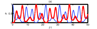
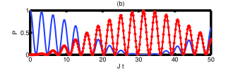
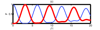
Figure 4: (Color online) The time evolution of the populations of the states $|\phi_{1}\rangle$ and $|\phi_{4}\rangle$ for the different coupling mechanisms (a) $J=\lambda$, (b) $J=10\lambda$, and (c) $J=0.1\lambda$. Solid-blue lines represent the population $|D_{1}(t)|^{2}$ of the state $|\phi_{1}\rangle$, while solid-dot-red lines indicate the the population $|D_{4}(t)|^{2}$ of the state $|\phi_{4}\rangle$.

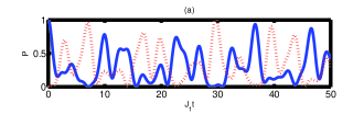
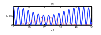
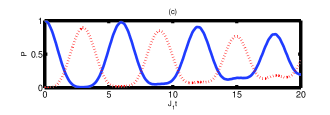
Figure 5: (Color online) The time evolution of the populations of the states $|\phi_{1}\rangle$ and $|\phi_{4}\rangle$ for the unbalanced coupling: (a) $\lambda_{1}=0.9J_{1},~{}\lambda_{2}=0.9J_{2},~{}J_{2}=0.9J_{1}$; (b) $J_{1}=10\lambda_{1},~{}J_{2}=10\lambda_{2},~{}\lambda_{1}=0.9\lambda_{2}$; (c) $J_{1}=0.1\lambda_{1},J_{2}=0.1\lambda_{2},\lambda_{1}=0.9\lambda_{2}$. Solid-blue lines represent the population $|D_{1}(t)|^{2}$ of the state $|\phi_{1}\rangle$, while red-dash lines indicate the the population $|D_{4}(t)|^{2}$ of the state $|\phi_{4}\rangle$.

Fidelity is a direct measure to characterize how accurate the QIT is achieved. Here, the fidelity is defined as $F=|\langle\Psi_{T}|\Psi(t)\rangle|^{2}$, where $|\Psi_{T}\rangle$ is the ideal target state of the transfer. The expression of the ideal target state is $|\Psi_{T}\rangle=|g\rangle_{NE_{1}}|0\rangle_{1}|0\rangle_{2}|0\rangle_{L}(\alpha|g\rangle+\beta|e\rangle)_{NE_{2}}$ for the resonant interaction, while $|\Psi_{T}\rangle=|g\rangle_{NE_{1}}|0\rangle_{1}|0\rangle_{2}(\alpha|g\rangle+\beta|e\rangle)_{NE_{2}}$ for the large detuning case. We obtain the expression of the fidelity $F=|\alpha|^{2}+|\beta C_{5}(t)|^{2}$ for the resonant interaction, while $F=|\alpha|^{2}+|\beta D_{4}(t)|^{2}$ for the large detuning case. As an example, let’s consider $\alpha=1/\sqrt{3}$ and $\beta=\sqrt{2/3}$. We have $F=(1+2|C_{5}(t)|^{2})/3$ for the resonant interaction case, while $F=(1+2|D_{4}(t)|^{2})/3$ for the large detuning case. The fidelities for the two cases are plotted in Fig. 6, which shows that high-fidelity QIT between the two NVCEs can be achieved at some moment.

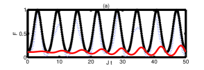
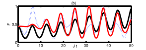
Figure 6: (Color online) Fidelity $F$ versus $Jt$, without considering the dissipation of the system. (a) Resonant interaction case. Dashed-blue, solid-dot-black, and solid-red curves correspond to $J=g$, $J=0.1g$, and $J=10g$, respectively. (b) Large detuning case. Dashed-blue, solid-black, and solid-red lines correspond to $J=\lambda$, $J=0.1\lambda$, and $J=10\lambda$, respectively.

It is meaning to investigating the influence of decoherence of the system on the QIT. When the dissipation of the system is considered, the dynamics of the lossy system is governed by the following master equation

$$\dot{\rho} = -i[H_{I},\rho]+\frac{\kappa}{2}(2a\rho a^{{\dagger}}-a^{{\dagger}}a\rho-\rho a^{{\dagger}}a)$$ (13)

$$+\sum_{j}[\frac{\gamma^{\prime}_{qj}}{2}(\sigma_{z}^{j}\rho\sigma_{z}^{j}-\rho)+\frac{\gamma^{\prime}_{Nj}}{2}(S_{z}^{j}\rho S_{z}^{j}-\rho)$$

$$+\frac{\gamma_{qj}}{2}(2\sigma_{j}^{-}\rho\sigma_{j}^{+}-\rho\sigma_{j}^{+}\sigma_{j}^{-}-\sigma_{j}^{+}\sigma_{j}^{-}\rho)$$

$$+\frac{\gamma_{Nj}}{2}(2S_{j}^{-}\rho S_{j}^{+}-\rho S_{j}^{+}S_{j}^{-}-S_{j}^{+}S_{j}^{-}\rho)],$$

for the resonant interaction. Here, $\kappa$ is the decay rate of the LC circuit, $\gamma^{\prime}_{qj}$ ($\gamma^{\prime}_{Nj}$) is the dephasing rate of the j-th flux qubit (NVCE), and $\gamma_{qj}$ ($\gamma_{Nj}$) is the relaxation rate of the j-th flux qubit (NVCE). For the large detuning case, the LC circuit has been adiabatic eliminated in Hamiltonian (9). Thus, the master equation is given by

$$\dot{\rho} = -i[H_{eff},\rho]+\sum_{j}[\frac{\gamma^{\prime}_{qj}}{2}(\sigma_{z}^{j}\rho\sigma_{z}^{j}-\rho)+\frac{\gamma^{\prime}_{Nj}}{2}(S_{z}^{j}\rho S_{z}^{j}-\rho)$$ (14)

$$+\frac{\gamma_{qj}}{2}(2\sigma_{j}^{-}\rho\sigma_{j}^{+}-\rho\sigma_{j}^{+}\sigma_{j}^{-}-\sigma_{j}^{+}\sigma_{j}^{-}\rho)$$

$$+\frac{\gamma_{Nj}}{2}(2S_{j}^{-}\rho S_{j}^{+}-\rho S_{j}^{+}S_{j}^{-}-S_{j}^{+}S_{j}^{-}\rho)].$$

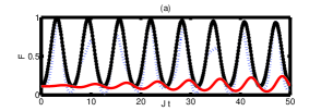
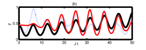
Figure 7: (Color online) Fidelity $F$ versus $Jt$, after taking the system dissipation into account. (a) Resonant interaction case. Dashed-blue, solid-dot-black, and solid-red curves correspond to $J=g$, $J=0.1g$, and $J=10g$, respectively. The plot was drawn by setting $\kappa=\gamma^{\prime}_{qj}=\gamma^{\prime}_{Nj}=\gamma_{qj}=\gamma_{Nj}=0.001J$. (b) Large detuning case. Dashed-blue, solid-black, and solid-red lines correspond to $J=\lambda$, $J=0.1\lambda$, and $J=10\lambda$, respectively. The plot was drawn by setting $\gamma^{\prime}_{qj}=\gamma^{\prime}_{Nj}=\gamma_{qj}=\gamma_{Nj}=0.001J$.

The Fig. 7 shows fidelity of the QIT versus $Jt$, after taking the dissipation of the system into account. Comparing Fig. 7 with Fig. 6, one can see that the influence of the dissipation of the system on the fidelity is negligible at small $Jt$.

Let us briefly discuss the experimental feasibility of our proposal. During the annealing process, a NVCE is created by ion implantation into a diamond. A diamond crystal is bonded on top of the flux qubit chip with its surface facing the chip a6 ; a7 . The size of a flux qubit is $1\mu$m order a5 . A physical system with multiple flux qubits coupled to a LC circuit has been proposed a11 . The time $t$ of the QIT is inverse ratio to the coupling strength $J$. For the coupling strength $J\approx 70$MHz, we have $t\sim 1/J\sim 14$ ns, which is much shorter than the flux qubit’s coherence time $T_{2}\simeq 20\mu$s h and the NVCE’s coherence time approaching $1$ second h1 . Also, decoherence of the flux qubits and the NVCEs can be effectively suppressed by periodic dynamical decoupling j .

IV Extending to the scalable quantum circuit

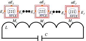
Figure 8: (Color online) Scalable quantum information transfer circuit. Multiple flux qubits are coupled to a LC circuit by their mutual inductances $M_{j}(j=1,2,...n)$. Each flux qubit couples to a NVCE acting as an information memory unit.

Our proposal can be extended to the scalable quantum circuit, which is constructed by $n$ flux qubits, NVCEs and a LC circuit acting as a data bus, shown in Fig. 8. All flux qubits can be made to be coupled (or decoupled) with the LC circuit by varying the external flux applied to each qubit loop. Alternatively, one can replace the small junction of each flux qubit with a SQUID and change external magnetic field threading the SQUID loop f0 ; f ; k , such that each flux qubit is coupled or decoupled to the LC circuit. In this way, the information can be transferred between any two selected NVCEs. Furthermore, the architecture provides the possibility for creating entanglement among NVCEs and performing quantum logic operations on NVCEs, which are important in quantum information processing.

V Conclusion

A hybrid architecture has been proposed for realizing QIT between NVCEs. For both resonant interaction and large detuning cases, it has been explicitly shown that high-fidelity QIT can be achieved between two spatially-separated NVCEs, and is robust against decoherence of the hybrid architecture. Also, a discussion has been given for the influence of the different coupling mechanisms on the QIT. According to the current experimental conditions, the feasibility of this proposed has been analyzed. The proposed architecture opens a way for scalable QIT among NVCEs, which is important in large scale quantum information processing. Finally, the method presented here is applicable to a wide range of physical implementation with different types of data buses such as nanomechanical resonators and TLRs.

- (1) L. M. Duan, M. D. Lukin, J. I. Cirac, and P. Zoller, Nature 414, 413 (2001).
- (2) S. B. Zheng and G. C. Guo, Phys. Rev. Lett. 85, 2392 (2000).
- (3) S. Osnaghi, P. Bertet, A. Auffeves, P. Maioli, M. Brune, J. M. Raimond, and S. Haroche, Phys. Rev. Lett. 87, 037902 (2001).
- (4) C. P. Yang, S. I Chu, and S. Han, Phys. Rev. A 67, 042311 (2003).
- (5) P. B. Li, Y. Gu, Q. H. Gong, and G. C. Guo, Phys. Rev. A 79, 042339 (2009).
- (6) J. W. Pan, Z. B. Chen, C. Y. Lu, H. Weinfurter, A. Zeilinger, and M. Żukowski, Rev. Mod. Phys. 84, 777 (2012), and references therein.
- (7) C. P. Yang, Q. P. Su, and F. Nori, New J. Phys. 15, 115003 (2013).
- (8) F. Y. Zhang, B. Liu, Z. H. Chen, S. L. Wu, and H. S. Song, Ann. Phys. (N.Y.) 346, 103 (2014).
- (9) I. Buluta, S. Ashhab, and F. Nori, Rep. Prog. Phys. 74, 104401 (2011).
- (10) J. Q. You and F. Nori, Phys. Today 58, 42 (2005); Nature 474, 589 (2011).
- (11) P. D. Nation, J. R. Johansson, M. P. Blencowe, and F. Nori, Rev. Mod. Phys. 84, 1 (2012).
- (12) L. Childress, M. V. Gurudev Dutt, J. M. Taylor, A. S. Zibrov, F. Jelezko, J. Wrachtrup, P. R. Hemmer, and M. D. Lukin, Science 314, 281 (2006).
- (13) P. Neumann, N. Mizuochi, F. Rempp, P. Hemmer, H. Watanabe, S. Yamasaki, V. Jacques, T. Gaebel, F. Jelezko, and J. Wrachtrup, Science 320, 1326 (2008).
- (14) G. Balasubramanian, P. Neumann, D. Twitchen, M. Markham, R. Kolesov, N. Mizuochi, J. Isoya, J. Achard, J. Beck, J. Tissler, V. Jacques, P. R. Hemmer, F. Jelezko, and J. Wrachtrup, Nature Mater. 8, 383 (2009).
- (15) F. Jelezko, T. Gaebel, I. Popa, A. Gruber, and J. Wrachtrup, Phys. Rev. Lett. 92, 076401 (2004).
- (16) P. C. Maurer, G. Kucsko, C. Latta, L. Jiang, N. Y. Yao, S. D. Bennett, F. Pastawski, D. Hunger, N. Chisholm, M. Markham, D. J. Twitchen, J. I. Cirac, and M. D. Lukin, Science 336, 1283 (2012).
- (17) Z. L. Xiang, S. Ashhab, J. Q. You, and F. Nori, Rev. Mod. Phys. 85, 623 (2013).
- (18) A. Imamoğlu, Phys. Rev. Lett. 102, 083602 (2009).
- (19) J. H. Wesenberg, A. Ardavan, G. A. D. Briggs, J. J. L. Morton, R. J. Schoelkopf, D. I. Schuster, and K. Mølmer, Phys. Rev. Lett. 103, 070502 (2009).
- (20) W. L. Yang, Z. Q. Yin, Y. Hu, M. Feng, and J. F. Du, Phys. Rev. A 84, 010301(R) (2011).
- (21) F. Y. Zhang, Y. Shi, C. Li, and H. S. Song, Eur. Phys. J. B 85, 385 (2012).
- (22) Y. Kubo, C. Grezes, A. Dewes, T. Umeda, J. Isoya, H. Sumiya, N. Morishita, H. Abe, S. Onoda, T. Ohshima, V. Jacques, A. Dréau, J.-F. Roch, I. Diniz, A. Auffeves, D. Vion, D. Esteve, and P. Berte, Phys. Rev. Lett. 107, 220501 (2011).
- (23) D. Marcos, M. Wubs, J. M. Taylor, R. Aguado, M. D. Lukin, and A. S. Sørensen, Phys. Rev. Lett. 105, 210501 (2010).
- (24) D. I. Schuster, A. P. Sears, E. Ginossar, L. DiCarlo, L. Frunzio, J. J. L. Morton, H. Wu, G. A. D. Briggs, B. B. Buckley, D. D. Awschalom, and R. J. Schoelkopf, Phys. Rev. Lett. 105, 140501 (2010).
- (25) Y. Kubo, F. R. Ong, P. Bertet,1 D. Vion, V. Jacques, D. Zheng, A. Dréau, J. F. Roch, A. Auffeves, F. Jelezko, J. Wrachtrup, M. F. Barthe, P. Bergonzo, and D. Esteve, Phys. Rev. Lett. 105, 140502 (2010).
- (26) X. Zhu, S. Saito, A. Kemp, K. Kakuyanagi, S. Karimoto, H. Nakano, W. J. Munro, Y. Tokura, M. S. Everitt, K. Nemoto, M. Kasu, N. Mizuochi, and K. Semba, Nature 478, 221 (2011).
- (27) S. Saito, X. Zhu, R. Amsüss, Y. Matsuzaki, K. Kakuyanagi, T. Shimo-Oka, N. Mizuochi, K. Nemoto, W. J. Munro, and K. Semba, Phys. Rev. Lett. 111, 107008 (2013).
- (28) Z. L. Xiang, X. Y. Lü, T. F. Lie, J. Q. You, and F. Nori, Phys. Rev. B 87, 144516 (2013).
- (29) J. Johansson, S. Saito, T. Meno, H. Nakano, M. Ueda, K. Semba, and H. Takayanagi, Phys. Rev. Lett. 96, 127006 (2006).
- (30) R. H. Koch, G. A. Keefe, F. P. Milliken, J. R. Rozen, C. C. Tsuei, J. R. Kirtley, and D. P. DiVincenzo, Phys. Rev. Lett. 96, 127001 (2006).
- (31) Y. X. Liu, et al., Phys. Rev. A 74, 052321 (2006); Phys. Rev. B 76, 144518 (2007).
- (32) A. Fedorov, A. K. Feofanov, P. Macha, P. Forn-Díaz, C. J. P. M. Harmans, and J. E. Mooij, Phys. Rev. Lett. 105, 060503 (2010).
- (33) Y. J. Zhao, X. M. Fang, F. Zhou, and K. H. Song, Phys. Rev. A 86, 052325 (2012).
- (34) Q. Chen, W. L. Yang, and M. Feng, Phys. Rev. A 86, 022327 (2012).
- (35) X. Y. Lü, Z. L. Xiang, W. Cui, J. Q. You, and F. Nori, Phys. Rev. A 88, 012329 (2013).
- (36) T. P. Spiller, K. Nemoto, S. L. Braunstein, W. J. Munro, P. van Loock, and G. J. Milburn, New J. Phys. 8, 30 (2006).
- (37) A. M. Stephens, J. Huang, K. Nemoto, W. J. Munro, Phys. Rev. A 87, 052333 (2013).
- (38) J. H. N. Loubser and J. A. van Wyk, Rep. Prog. Phys. 41, 1201 (1978).
- (39) P. Neumann, R. Kolesov, V. Jacques, J. Beek, J. Tisler, A. Batalov, L. Rogers, N. B. Manson, G. Balasubramanian, F. Jelezko, and J. Wrachtrup, New J. Phys. 11, 013017 (2009).
- (40) T. P. Orlando, J. E. Mooij, L. Tian, C. H. van der Wal, L. S. Levitov, S. Lloyd, and J. J. Mazo, Phys. Rev. B 60, 15398 (1999).
- (41) J. E. Mooij, T. P. Orlando, L. Levitov, L. Tian, C. H. wan der Wal, and S. Lloyd, Science 285, 1036 (1999).
- (42) J. Bylander, S. Gustavsson, F. Yan, F. Yoshihara, K. Harrabi, G. Fitch, D. G. Cory, Y. Nakamura, J. S. Tsai, and W. D. Oliver, Nature Phys. 7, 565 (2011).
- (43) N. Bar-Gill, L.M. Pham, A. Jarmola, D. Budker, and R.L. Walsworth, Nature Comm. 4, 1743 (2013).
- (44) W. Yang, Z. Y. Wang, and R. B. Liu, Front. Phys. 6, 2 (2011), and references therein.
- (45) X. Zhu, A. Kemp, S. Saito, and K. Semba, Appl. Phys. Lett. 97, 102503 (2010).