Ripples in hexagonal lattices of atoms coupled to Glauber spins
Abstract
A system of atoms connected by harmonic springs to their nearest neighbors on a lattice is coupled to Ising spins that are in contact with a thermal bath and evolve under Glauber dynamics. Assuming a nearest-neighbor antiferromagnetic interaction between spins, we calculate analytically the equilibrium state. On a one-dimensional lattice, the system exhibits first and second order phase transitions. The order parameters are the total magnetization and the number of spin pairs in an antiferromagnetic configuration. On a hexagonal two dimensional lattice, spins interact with their nearest-neighbors and next-nearest-neighbors. Together with the coupling to atoms, these interactions produce a complex behavior that is displayed on a phase diagram. There are: ordered phases associated to ripples with atomic wavelength and antiferromagnetic order, ordered phases associated to ripples with nanometer wavelengths and ferromagnetic order, disordered glassy phases, and other phases presenting stripes formed by different domains. These static phases are discussed in relation to existing experiments and results for other models found in the literature.
1 Introduction
Graphene is a one-atom thick crystal membrane with extraordinary mechanical and electronic properties [1, 2, 3]. Experimental characterization of suspended graphene shows that it is covered with ripples. These ripples are several nanometers long waves of the sheet without a preferred direction [4, 5], modify the electronic band structure [6], and are expected to be relevant in the understanding of electronic transport in graphene [7]. Also, more recently, buckling in which the unit structures consist of only two-three unit cells of the graphene honeycomb lattice has been experimentally observed [8].
There have been many studies of ripples. The earliest studies using Monte Carlo [9] or molecular dynamics simulations [10] have shown that ripples may be connected to variable length bonds of carbon atoms and may be caused by thermal fluctuations. Other studies have explored the connection between rippling and electron-phonon coupling [11, 12]. In particular, it has been suggested that, at zero temperature, the electron-phonon coupling may drive the graphene sheet into a quantum critical point characterized by the vanishing of the bending rigidity of the membrane [13]. The continuation of this work by J. Gonzalez [14] discusses the nonzero expectation value of the mean curvature (the Laplacian of the flexural phonon field) once the bending rigidity of the membrane vanishes, and its role as order parameter. Alternatively, assuming that the graphene membrane is fluctuating in dimensions (with ), Guinea et al. have calculated the dressed two-particle propagators of the elastic and electron interactions. They have found a collective mode which becomes unstable at a nonzero wave vector and causes the appearance of Gaussian curvature [15]. Amorim et al. [16] estimate the crossover temperature between quantum and classical descriptions to be 70-90 K. Thus a quantum description of ripples is not necessary at room temperature. All these studies investigate and characterize rippling as equilibrium phenomena.
We are interested in rippling dynamics and stability of static corrugations under disturbances. In experiments to visualize ripples using a transmission electron microscope (TEM), the suspended graphene sheet is hit by a low-intensity electron beam that may push atoms out-of-plane upward or downward in a random fashion. An alternative technique to visualize ripples is using a scanning tunneling microscope (STM)[17]. In this case, the graphene sheet is pushed and locally heated in the region close to the tip. Depending on the tunneling current and the voltage between tip and sheet, the latter may undergo a phase transition from a flexible (rippled) to a rigid (buckled) state [18].
In Ref. [19], the authors simplify the distortion of the d crystal by modeling it with two-state spin-like variables ( upward, downward). There are antiferromagnetic interactions among these spins, because the out-of-plane shift of the atoms in opposite directions stabilize the strictly d system while keeping the gapless band structure of graphene [19]. A rich phase diagram is found, including paramagnetic, ordered and glassy phases, depending on the temperature and the values of the nearest-neighbor and next-nearest-neighbor couplings. In this way, they describe the formation and origin of the atomic scale rippling found in Ref. [8]. On the other hand, there are also models that investigate rippling by considering at each lattice site a continuous variable describing the out-of-plane displacement of the carbon atom coupled to a spin variable () representing an internal degree of freedom [20, 21]. This may be understood as a mechanical system coupled to a spin system. The spin at each lattice site represents the non-saturated fourth bond that, by a physical mechanism similar to the one discussed in [19], tries to pull the corresponding atom upward () or downward () from the flat sheet configuration. Mathematically, this is done by introducing a linear coupling term in the system energy, proportional to for each lattice site. In these simple models, the mechanical system is either a chain of oscillators [20] or a discrete elasticity model of the hexagonal graphene lattice [21], while the spins are in contact with a thermal bath and flip randomly according to Glauber dynamics at the temperature of the thermal bath. In both models, the system forms metastable but long-lived ripples assuming slow spin relaxation [20, 21].
It is worth investigating a combination of the two approaches described in the previous paragraph. Firstly, it seems sensible to model the out-of-plane displacement at each lattice site by a continuous variable as in Refs. [20, 21], which is driven by the internal degree of freedom represented by the spin. Secondly, these spins certainly interact among themselves, by the mechanism proposed in [19]. Thus, in this paper we discuss the formation and dynamics of ripples in graphene through a system of atoms connected by harmonic springs and coupled to interacting Ising spins. We start from the spin-oscillator chain model [20, 21, 22] and add interactions among spins that produce stable rippling states. There appear different phases and transitions between them depending on parameter values.
The plan of the paper is as follows. In Section 2, we introduce the one-dimensional model and calculate analytically the equilibrium state. We also present the equations that determine the dynamics of the system. Section 3 is devoted to the expansion of the model to dimensions on a hexagonal lattice, with first and second-neighbors interactions between spins. Besides, we do a systematic analysis of the system modifying the parameters and studying the stationary configuration after the transitory, using a phase diagram in Section 3.1, and describing the different phenomenology of each phase in Section 3.2. The main conclusions are presented in Sec. 4. Relevant information that is not covered in the main text is presented in the Appendices: some geometrical expressions for the hexagonal lattice are discussed in A, while images of the different phases are collected in B.
2 The one-dimensional model
To start with, we consider a one-dimensional chain of oscillators with nearest-neighbor interactions, in which each oscillator is linearly coupled to an Ising spin . A detailed investigation of this model can be found in Ref. [20]. Therein, it was shown that, for appropriate temperatures, the stable equilibrium configuration has only one ripple, although there appeared some more complex long-lived metastable rippled states. To explore whether stable multi-rippled equilibrium configurations are possible, we add an anti-ferromagnetic term to the hamiltonian,
| (1) |
Here and are the vertical displacement and momentum respectively, and the extreme oscillators and spins are fixed () [23]. The dynamics of the model is as follows: (i) the oscillators’ equations of motion,
| (2) |
are the usual ones, whereas the spins evolve according to Glauber dynamics [24]. The transition rate from the configuration to (obtained from by flipping the -th spin) is
| (3) | |||
| (4) |
in which is the characteristic attempt rate for the spin flips. The Glauber transition rates ensure that the system satisfies detailed balance, and therefore the system reaches equilibrium for long enough times. In equilibrium, the probability of a certain configuration is proportional to , where we measure the temperature in units of energy.
As explained in [20], for rippling appears provided the temperature is less than
| (5) |
as . To guarantee that the diffusive term in (2) remains finite in the continuum limit, it is convenient to nondimensionalize the equations of motion as follows:
| (6) | |||
| (7) |
Then the transition rates and the equations of motion become
| (8) |
We will omit the asterisks in nondimensional equations from now on. In order to obtain the scaling of the critical temperature, we need to know the scaling of the model parameters with the system size. In principle, this could be done by deriving our model from a fundamental microscopic one, but this is outside the scope of this paper. Nevertheless, we discuss some possible scalings in the following. If both the elastic constant and the antiferromagnetic coupling constant are considered to be independent of the system size, the only remaining parameter is , the coupling between the elastic and internal (spin) degrees of freedom. If is also independent of the system size, the critical temperature diverges as . In this case, rippling would be observed at all temperatures. On the other hand, a finite value of in the large system size limit is obtained when . Then, rippling would be observed only for . In principle, both situations are compatible with current experiments, in which rippling is observed over a wide temperature range.
Let us consider now the equilibrium situation. Equation (8) can be averaged, with the result
| (9) |
in which and are the equilibrium average height and spin at position ; the system has unit size in the continuous space variable , . Therefore, the average curvature of the ripples is directly linked to the average spin. Very recently, this idea has been used to develop a phenomenological Ising model to study rippling in graphene in scanning tunneling microscopy experiments, in which each spin represents a whole ripple and the spin sign gives its corresponding convexity [18]. Interestingly, we can derive an effective free energy for the string, by integrating the canonical distribution over the momenta and the spins : the resulting probability becomes a functional of the string profile , which in dimensionless variables reads [25]
| (10a) | |||
| (10b) |
The quantity is the logarithm of the spins partition function per site, which depends on the “field” and the coupling . The particularization of this free energy to the case was obtained in Ref. [20]. For , in order to calculate , the system is divided into a set of nearly independent subsystems with sites each, but such that and the “field” can be considered almost constant within each subsystem. We may denote the subsystems by , in which corresponds to the position of the subsystem in the continuum limit. In each subsystem, the local average magnetization and correlation are given by the usual formulas
| (11) |
as plays the role of the external field and is the coupling constant. Global order parameters may be defined as
| (12) |
in which is the absolute value of the total magnetization per site and the fraction of spin pairs in an antiferromagnetic configuration is () for perfect antiferromagnetic (ferromagnetic) ordering.
Equation (10) clearly shows that the free energy is an extensive quantity if the dimensionless variables are of the order of unity, which is consistent with our scalings. Taking into account the expressions for the free energy, Eq. (10), and the average magnetization, Eq. (11), the equation giving the equilibrium profile (9) is nothing but the Euler-Lagrange equation for the free energy functional, as it should be: the string profile minimizes the free energy.
In what follows, we summarize the main physical implications of the short-ranged antiferromagnetic interaction, as compared to the case. The flat profile is always a solution of Eq. (9), but it becomes unstable for . For , there appear rippled configurations with non-zero magnetization that are stable for [20]. For the bifurcation condition produces two temperatures and for , as seen in the left panel of Fig. 1. Specifically, these rippled configurations become unstable for low (high) enough temperatures, (). The transitions at and are of second order, the order parameters and are continuous because bifurcates continuously from the solution , similarly to the behaviour found in the case. For , this rippled ferromagnetic phase no longer exists because the antiferromagnetic coupling is too strong.
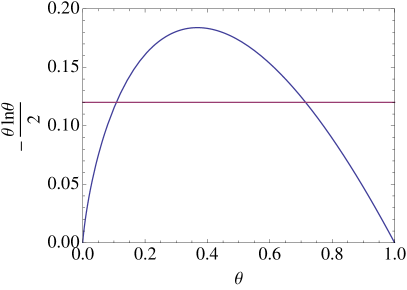
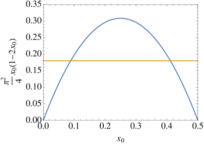
In the limit , the partition function of the spins becomes
| (13a) | |||
| (13b) |
where is the Heaviside step function, for and for , and is the sign function, . In the flat configuration, and everywhere. There appears a new rippled low temperature phase, that is antiferromagnetic near the boundaries because of the clamped boundary conditions. Inside an interval of length close to the boundaries, , and , therein. Then, the simplest configuration is composed of (i) two straight lines () near the boundaries, that is, in the intervals and , and (ii) a parabolic ripple with () in between, for , which corresponds to ferromagnetic ordering because and for . The continuity of and at implies that , which determines two possible values of for , as seen in the right panel of Fig. 1. The configuration corresponding to the smallest value is the absolute minimum of the free energy for , whereas both the flat string and the configuration corresponding to are metastable. For , the absolute minimum of the free energy corresponds to the flat string, whereas both configurations corresponding to and are metastable. The transition at (which corresponds to percent of the spins being antiferromagnetic) is first order, because the order parameters and change discontinuously: in the zero temperature flat configuration, it is and , whereas in the rippled state we have and . Moreover, as is usually the case in first-order phase transitions, the string has many other metastable configurations: they have internal nodes , , at which changes sign. The existence of the different phases and their relative stability will be thoroughly discussed elsewhere [25].
3 The two-dimensional model
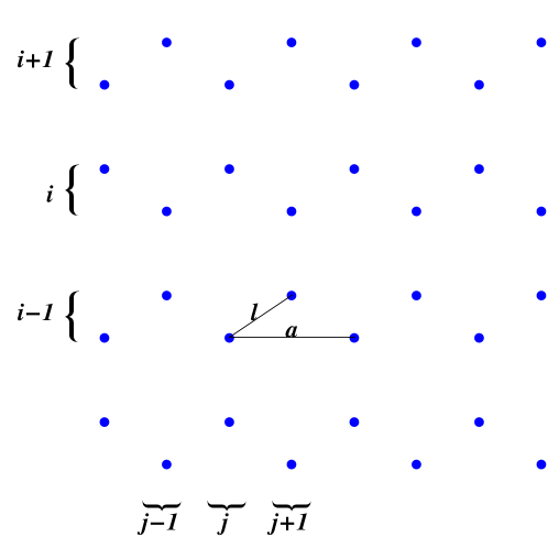
Here, we extend the model to dimension , in the hope that this will make it possible to find more complex behaviors. This extension is almost direct and, as we are interested in applying the model to mimic a graphene sheet, we consider a hexagonal lattice. Due to the symmetry, it is important to write the hamiltonian carefully. First, each atom is indexed: will be the row index and the column index, with the peculiarity that each row comprises atoms with two different heights in a zigzag distribution, see Figure 2. It is important to note that the form of the equations will be qualitatively different for atoms for which is an even number (e-atoms), which have one nearest neighbor above and two below, and those for which is an odd number (o-atoms), which have one nearest neighbor below and two above, that is, the opposite situation. It is quite obvious that if the plane is rotated by an angle of , the two types of atoms are interchanged.
Taking into account the notation described above, we can write down the extension of the 1 Hamiltonian to . Moreover, we introduce next-nearest-neighbor interactions,
| (14) | |||||
where and take values and , respectively. Following the same steps as in the previous section, the nondimensional equation of motion for each atom and the expressions for the transition rate become
| (15) |
| (16) |
| (17) | |||||
where is a large scale parameter to be calculated later. As we said before, the difference between e-atoms with o-atoms follows from the rotation by of the plane. For that reason, only equations for e-atoms have been written. In the latter equations, the height variable and time are dimensionless. In the nondimensionalization, the same parameters as in equations (6) and (7) appear, with the addition of , which corresponds to the new next-nearest-neighbor interaction.
The length of each side of the finite hexagonal lattice is , where is the side of a unit hexagonal cell and is the maximum value of the row index in Fig. 2. Let us measure all lengths in units of , so that tends to zero as the hexagonal lattice fills the plane. Then the expression within parenthesis in (15) has the limit [26, 27, 21]
| (18) |
as . Therefore, we take proportional to , namely
| (19) |
to guarantee that the diffusive term in (15) remains finite as (continuum limit). Note that the increments of the continuous variables are and , as seen in Fig. 2, so that the hexagonal lattice goes to the unit square in the continuum limit. For details, see A.
Once the system reaches the stationary state, equation (15) can be averaged ignoring thermal fluctuations. Thus, using equation (18) for we get
| (20) |
where and are the average height and spin at the point of the unit square. For , we have that and the flat configuration becomes unstable at , similarly to the situation in the 1d case. This kind of rigidly buckled configurations have been observed in graphene in recent STM experiments [18]. Equation (20) tells us that there is a correspondence between lattice patterns given by the average height profile and the spin configuration. Specifically, the curvature of the rippling is directly proportional to the average spin. Therefore, in the following section we will mainly characterize the phases by the spin configuration.
3.1 Phase diagram
As it has already been said, the stable steady state is a rigidly buckled configuration below the critical temperature (), provided there is no interaction between spins. We expect that the introduction of the nearest neighbour interaction among the spins should introduce new phases. By analogy with the 1d system, an antiferromagnetic nearest neighbour interaction should make antiferromagnetic ordered phases to appear for low enough temperatures. Looking for a more complex phenomenology, we introduce a next-nearest-neighbor interaction, as in Ref. [19]. This term appears in (14) through and in (17) through its dimensionless counterpart .
It is important to note that both () and () may take positive or negative values, corresponding to antiferromagnetic and ferromagnetic interactions, respectively. However, only positive values of will be considered, since a next-nearest-neighbor ferromagnetic interaction just strengthens the nearest-neighbor one [28]. For positive values of and the qualitative behavior is quite different. The nearest-neighbor interaction provides a defined minimum energy distribution in which each spin and its nearest-neighbors point in opposite directions. However, the next-nearest-neighbor interaction does not yield a defined minimum energy distribution. In fact, the second-neighbors of each atom are second-neighbors to each other, and therefore the next-nearest-neighbor interaction causes the system to be frustrated [19]. An enlightening discussion about frustration is given in the introduction of [29]. In principle, it is tempting to exclude negative values of from the analysis. On intuitive grounds, one may conclude that the nearest-neighbour ferromagnetic coupling with should only strengthen the already long-ranged ferromagnetic interaction among the spins induced by the spin-lattice coupling term [20]. Nevertheless, the situation is a little bit more complex, as discussed below.
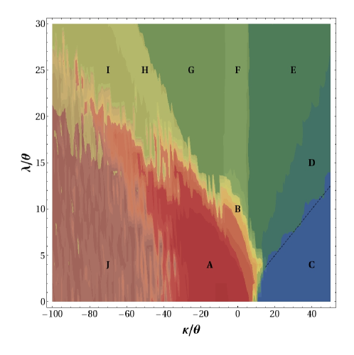
We plot a phase diagram to show in only one graph all the different behaviors, see Figure 3. In our simulations, we have chosen a nondimensional temperature , which is far below critical for . A key parameter is
| (21) |
where denotes the number of atoms in the lattice. This parameter estimates the domain-wall length [19], and it is equal to (resp. ) for completely ferromagnetic (resp. antiferromagnetic) behavior. In addition, to delimit the regions on the diagram, we have used the absolute value of the usual magnetization
| (22) |
and energy fluctuations (proportional to the specific heat),
| (23) |
Here is the system energy and , where the angular brackets stands for the mean value that is calculated once the stationary state has been reached.
3.2 Region characterization
The different regions in the phase diagram have been characterized using the three parameters , and . Figure 3 is the superposition of the projections of and on the plane . Each region of the plane correspond to different combinations of and values. Once the regions have been delimited using the magnitudes described above, the system is allowed to evolve with and in one of the regions. Next, we verify that the system reaches the equilibrium state and we obtain the basic structures in the spin domains. Moreover, to check that we have actually reached the equilibrium state, another simulation is carried out with this distribution as the initial condition: if, aside from thermal fluctuations, no evolution is found, equilibrium has been reached.
-
•
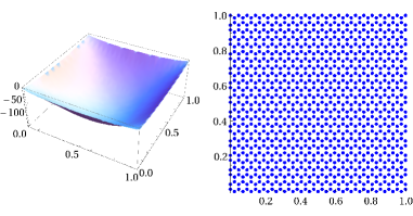
Region . , . The plane is completely curved, and the spins are all pointing in the same direction. This situation corresponds to small values of and , for which the interaction that dominates is the one between the surface and the spins, in agreement with the simple picture already present in the 1 model, see Section 2.
-
•
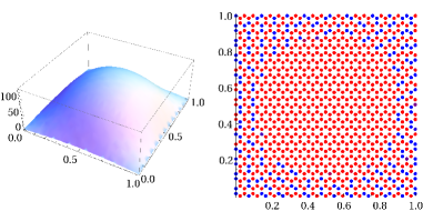
Region . It is the zone surrounding , on which and decrease from the values to those on the other regions. Here, the system displays a behavior that is analogous to the one described at the end of Section 2 (in 1). The interaction between the surface and the spins is an effective ferromagnetic interaction with an intensity that decreases from the center to the border. Thus, the plane is curved but the spins close to the border are antiferromagnetically arranged.
-
•
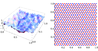
Region . , . The predominant interaction is the antiferromagnetic first-neighbor one. The equilibrium state (starting from a random initial spin distribution) is composed of antiferromagnetic domains.
-
•
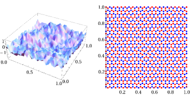
Region . increases from to , . The states in this region are metastable. Taking the distribution corresponding to the equilibrium state of or as the initial condition, the system does not evolve to the other state, at least in a simulation time much greater than the relaxation time from random initial conditions.
-
•
Region . , . In this case, the spins are distributed in rows of two atoms in the lowest energy configuration. Beginning with random initial conditions, these two-atoms domains were created, with the rows in any of the three symmetrical directions.
-
•
Region . , . The interaction between the plane and the spins is relevant again, since the antiferromagnetic next-nearest-neighbor interaction (with ) has no defined minimum energy distribution. The plane is curved, leading to a non-zero magnetization.
-
•
Region . , . The typical equilibrium configurations are long serpentine lines, with zero magnetization. Taking as initial conditions the spins arranged in rows, the system remains static.
-
•
Regions and . In them, the system evolves from the characteristic configurations of to the ferromagnetic configurations of , with the difference that in the magnetization is different from zero whereas in it is not. is a ferromagnetic first-neighbor state, but with domains smaller than in ( smaller than in ).
-
•
Region . , . In this case the system behaves as a completely ferromagnetic first-neighbor system. Starting from random initial conditions, ferromagnetic domains grow until reaching a stationary state. In this case is close to zero since spins are pointing to different directions in adjoining domains.
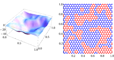
The plots of the typical equilibrium configurations for each region are in B.
It should be noted that our phase diagram does not contain a paramagnetic state because the chosen temperature, , is far below the critical temperature for and (unity in our dimensionless variables). Each point of the phase diagram corresponds to the energy minimum to which the system evolves for the considered parameters. Once it is in the neighborhood of this minimum, the energy barriers are so high that ergodicity is no longer valid, and the system remains frozen [30]. This causes an Edwards-Anderson order parameter [31],
| (24) |
to be different from zero at every point of the plotted phase diagram. On the other hand, close to , the order parameter will vanish as , once ergodicity is recovered. In Eq. (24) the average should be understood as a time average or an extended Gibbs average in a phase space composed of disjoint ergodic components [30].
4 Conclusions
We have studied a system of atoms connected by harmonic springs and coupled to Glauber spins. The spins are in contact with a thermal bath and interact with their neighbors. The system forms one ripple and becomes antiferromagnetic at the boundaries as increases, until it becomes completely antiferromagnetic. When the system is on a hexagonal lattice, each spin interacts with its nearest-neighbors and next-nearest-neighbors, aside from the coupling with the out-of-plane displacement. This situation generates different phases which are included in a phase diagram.
The range of parameters in our phase diagram includes negative values for the nearest neighbor coupling constant and is thus wider than the one used in [19], in which only antiferromagnetic interactions were considered. The change in the sign of the spin-spin interaction can be produced by the scattering of the conduction electrons at the spins, see [32, 33]. We are interested in zero magnetization phases since they correspond to no overall bending. Our model provides different phases obeying this constraint: I and J are long wave length phases, similar to those observed in [4, 5], whereas C, E and G are phases with atomic wave length. G is a stripy phase (see Figure 4), which could be associated with patterns seen in [8]. The atomic wave length phases C and E correspond with phases Ordered 1 and 2, respectively, from Ref. [19]. Therein, the line between these two phases is (in our variables) , which agrees with the limit of true stability of C here. Interestingly, neither the metastable phase or the other phases (including the long wavelength phases I and J) were found in Ref. [19]. In that reference, (i) only positive values of were considered, and (ii) there was no spin-atom coupling.
The buckling phase A is surrounded by rippled phases C, E, and G with no overall bending. Starting from a point of the phase diagram belonging to region C (rippled phase), if we increase the temperature while keeping and (supposed temperature independent) fixed, we move along a straight line of slope in Figure 3 from phase C to the buckled phase A. In experiments with STM at fixed current, the temperature is locally increased at the tip region and this triggers a transition from a rippled flexible phase to a rigid buckled phase [18]. Thus our model contains the ripples-to-buckling transition observed in experiments although more work needs to be done to explain STM observations in detail [25].
To conclude, our model is based in a few parameters controlling simple interactions which generate complex collective behaviors. This allows us to identify the interactions responsible for each pattern. In addition, the elastic feature of the model makes it possible to visualize and quantify the magnitude of the rippling, which could be compared with experiments once height measurements had been improved.
Appendix A Geometrical expressions
We want our hexagonal lattice to have equal overall length and height. Let be the total number of rows. Then
| (25) |
is the total number of columns, and the height of the hexagonal lattice is
| (26) |
where is the length of the side of a unit hexagonal cell. With these expressions, if , then and the vertical and horizontal side of the lattice are and respectively, in units of . Our finite hexagonal lattice is then roughly inscribed in a square and the nondimensional side of the unit hexagonal cell is .
Appendix B Phase diagram images
In our simulations, we have used a lattice of 2,150 atoms and a temperature . We need to impose initial and boundary conditions for the membrane and the spins. Initially, the spins are in a completely random configuration, whereas the membrane is flat and at rest. The membrane is clamped (zero displacement) at the boundaries. As nearest and next-nearest neighbors determine the dynamics of a given spin, see eq. (17), a spin located next to the boundary condition needs data from nearby spins located at the boundaries and also outside the lattice. The simplest possibility is that the spins of clamped boundary atoms and their nearest neighbors outside the lattice do not interact with the others, which can be achieved by formally assigning spin zero to them.
A
 B
B
C
 E
E
F
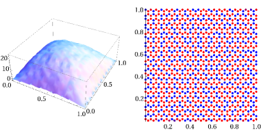 G
G
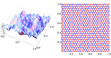
H
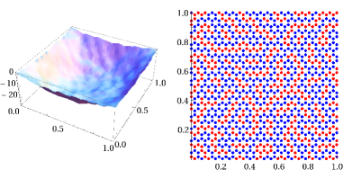 I
I
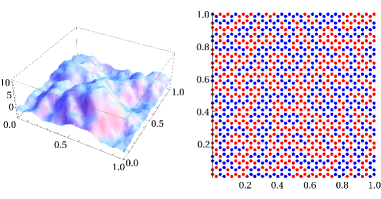
J
References
- [1] Novoselov K S, Geim A K, Morozov S V, Jiang D, Y. Zhang Y, Dubonos S V, Grigorieva I V and Firsov A A, 2004 Science 306 666
- [2] Novoselov K S, Jiang D, Schedin F, Booth T J, Khotkevich V V, Morozov S V and Geim A K, 2005 Proc. Natl. Acad. Sci. USA 102 10451
- [3] Castro Neto A H, Guinea F, Peres N M R, Novoselov K S, and Geim A K, 2009 Rev. Mod. Phys. 81 109
- [4] Meyer J C, Geim A K, Katsnelson M I, Novoselov K S, Booth T J and Roth S, 2007 Nature 446 60
- [5] Bangert U, Gass M H, Bleloch A L, Nair R R, and Geim A K, 2009 Physica status solidi (a) 206 1117
- [6] Guinea F, Horovitz B and Le Doussal P, 2008 Phys. Rev. B 77 205421
- [7] Katsnelson M I and Geim A K, 2008 Phil. Trans. R. Soc. A 366 195
- [8] Mao Y, and Wang W L, Wei D, Kaxiras E, and Sodroski J G, 2011 ACS Nano. 5 1395
- [9] Fasolino A, Los J H and Katsnelson M I, 2007 Nature Materials 6 858
- [10] Abedpour N, Neek-Amal M, Asgari R, Shahbazi F, Nafari N and Tabar M R, 2007 Phys. Rev. B 76 195407
- [11] Kim E A and Castro Neto A H, 2008 Europhys. Lett. 84 57007
- [12] Gazit D, 2009 Phys. Rev. B 80 161406(R)
- [13] San-Jose P, González J and Guinea F, 2011 Phys. Rev. Lett. 106 045502
- [14] González J, 2014 Phys. Rev. B 90 165402
- [15] Guinea F, Le Doussal P and Wiese K J, 2014 Phys. Rev. B 89 125428
- [16] Amorim B, Roldán R, Cappelluti E, Fasolino A, Guinea F and Katsnelson MI, 2014 Phys. Rev. B 89 224307
- [17] R. Zan, C. Muryn, U. Bangert, P. Mattocks, P. Wincott, D. Vaughan, X. Li, L. Colombo, R.S. Ruoff, B. Hamilton and K.S. Novoselov, 2012 Nanoscale 4, 3065
- [18] J.K. Schoelz, P. Xu, V. Meunier, P. Kumar, M. Neek-Amal, P. M. Thibado, and F. M. Peeters, 2015 Phys. Rev. B 91, 045413
- [19] O’Hare A, Kursmartsev F V and Kugel K I, 2012 Nano Lett. 12 1045
- [20] Bonilla L L, Carpio A, Prados A and Rosales R R, 2012 Phys. Rev. E 85 031125
- [21] Bonilla L L and Carpio A, 2012 J. Stat. Mech.: Theor. Exp. P09015
- [22] Prados A, Bonilla L L and Carpio A, 2010 J. Stat. Mech.: Theor. Exp. P06016; Bonilla L L, Prados A and Carpio A, 2010 J. Stat. Mech.: Theor. Exp. P09019
- [23] We take the spins at the boundaries formally equal to zero because it is the simplest choice. Alternatively, this boundary condition may be understood as if there were no spin associated to the clamped displacements . From either point of view, the term corresponding to the spin-oscillator and the spin-spin interactions in eq. (1) become , which only involve the “bulk” sites .
- [24] Glauber R J, 1963 J. Math. Phys. 4 294
- [25] Ruiz-García M, Bonilla L L, and Prados A, to be published.
- [26] Carpio A and Bonilla L L, 2008 Phys. Rev. B 78 085406
- [27] Bonilla L L and Carpio A, 2012 Phys. Rev. B 86 195402
- [28] For both ferromagnetic and antiferromagnetic ordering, the next-nearest-neighbors of a given spin are parallel to it.
- [29] Mezard M, Parisi G and Virasoro M A, 1987 Spin glass theory and beyond, (Singapore: World Scientific)
- [30] Heidelberg Colloquium on Glassy Dynamics, (Van Hemmen J L and Morgenstern I, ed.), 1983 Lect. N. Phys. 192 203-233
- [31] Edwards S F, and Anderson P W, 1975 Journal of Physics F: Metal Physics 5 965
- [32] Ruderman R A and Kittel C, 1954 Physical Review 96 99
- [33] Binder K and Young A P, 1986 Reviews of Modern Physics 58 4