Non-monotonicity of trace distance under tensor products

Abstract

The trace distance (TD) possesses several of the good properties required for a faithful distance measure in the quantum state space. Despite its importance and ubiquitous use in quantum information science, one of its questionable features, its possible non-monotonicity under taking tensor products of its arguments (NMuTP), has been hitherto unexplored. In this article we advance analytical and numerical investigations of this issue considering different classes of states living in a discrete and finite dimensional Hilbert space. Our results reveal that although this property of TD does not shows up for pure states and for some particular classes of mixed states, it is present in a non-negligible fraction of the regarded density operators. Hence, even though the percentage of quartets of states leading to the NMuTP drawback of TD and its strength decrease as the system’s dimension grows, this property of TD must be taken into account before using it as a figure of merit for distinguishing mixed quantum states.

1 Introduction

Quantifiers for the distance (distinguishability) between two density operators in the quantum state space $\mathcal{D}(\mathcal{H})$–the space formed by positive semidefinite matrices with trace equal to one–are an essential and frequently used item in the quantum information scientist toolkit Nielsen_Book ; Wilde_Book ; Fuchs_PhD . For instance, how well a quantum system was prepared Watanabe_QSP , manipulated Walter_EOWQC or protected Laflamme_QEC in an experiment is usually evaluated via how close (how indistinguishable) its real state is from what one would ideally expect. Distance measures in $\mathcal{D}(\mathcal{H})$ naturally appear also in the contexts of quantum foundations Gisin_cloning ; Wilde_U_Mem ; Zurek_qcb1 , quantum processes Cory_QP ; Nielsen_QP , quantum cryptography Fuchs_Cryp ; Gisin_RevQC , quantum phase transitions Gu_RevF , quantum speed limits Plastino_QSL ; Kok_QSL ; Davidovich_QSL ; Lutz_QSL ; Plenio_QSL ; Fan_QSL , quantum channel capacities Giovannetti_Channels , and also in the theories of quantum entanglement Horodecki_RevE ; Davidovich_RevE , quantum discord Lucas_RevD ; Vedral_RevD ; Streltsov_B , and quantum coherence Plenio_QC ; Aberg_QC ; Girolami_QC ; Zhao_QC .

Several distance (distinguishability) measures in the quantum state space have been proposed in the literature in the last decades. A partial list is provided in Ref. Audenaerte_DM . A few examples are the Bures’ distance, that is defined in terms of a similarity measure known as Uhlmann’s fidelity Bures ; Uhlmann_F (for a critical assessment regarding the use of this function in quantum information science see Ref. Paris_F ), the $p-$norm distance, with the trace distance (or $1-$norm distance) and the Hilbert-Schmidt distance (or $2-$norm distance) being used more frequently (see Refs. Petz_p_norm ; Sarandy_1Norm_D ; Sarandy_DSC_exp ; Vedral_2Norm_D and references therein), the quantum relative entropy Umegaki_QRE ; Petz_QRE ; Vedral_QRE ; Maziero_dist_MI , and the quantum Chernoff bound Szkola_QCB ; Acin_QCB , with these last two distinguishability measures being defined operationally, respectively, in the contexts of asymmetric and symmetric quantum hypothesis testing.

In this article we are interested mainly in one of the most popular distance measures, the trace distance, that is defined using the trace norm. For a Hermitian matrix $A$, the trace norm is defined and given as follows:

$$||A||_{1}:=\mathrm{Tr}\sqrt{A^{\dagger}A}=\mathrm{Tr}\sqrt{A^{2}}={\textstyle\sum_{j}}|a_{j}|,$$ (1)

with $|a_{j}|$ being the absolute value of the real eigenvalues of $A$. We can quantify how dissimilar two density operators $\rho$ and $\zeta$ are by their trace distance (TD), which is defined as the trace norm of their subtraction,

$$d_{tr}(\rho,\zeta):=||\rho-\zeta||_{1},$$ (2)

and assumes values between zero and two Wilde_Book .

This mathematical function possesses several of those properties required for a faithful distance (distinguishability) measure in the quantum state space Nielsen_Book ; Wilde_Book : For the density operators $\rho$, $\zeta$, and $\alpha$, the trace distance is, e.g., positive semidefinite ($d_{tr}(\rho,\zeta)\geq 0$), it is zero if and only if the two density operators are equal ($d_{tr}(\rho,\zeta)=0\Leftrightarrow\rho=\zeta$), it is symmetric ($d_{tr}(\rho,\zeta)=d_{tr}(\zeta,\rho)$), it obeys the triangle inequality ($d_{tr}(\rho,\zeta)\leq d_{tr}(\rho,\alpha)+d_{tr}(\alpha,\zeta)$), it is invariant under unitary transformations ($d_{tr}(\rho,\zeta)=d_{tr}(U\rho U^{\dagger},U\zeta U^{\dagger})$ for $UU^{\dagger}=\mathbb{I}_{d}$, where $\mathbb{I}_{d}$ is the $d\mathrm{x}d$ identity matrix), it leads to the equality $d_{tr}(\rho\otimes\alpha,\zeta\otimes\alpha)=d_{tr}(\rho,\zeta)$, it is monotonic under discarding subsystems ($d_{tr}(\rho_{1},\zeta_{1})\leq d_{tr}(\rho_{12},\zeta_{12})$ with $x_{1}=\mathrm{Tr}_{2}(x_{12})$), and it is consequently also monotonic under trace-preserving quantum operations ($d_{tr}(\rho,\zeta)\geq d_{tr}(\Phi(\rho),\Phi(\zeta))$ with $\Phi(x)={\textstyle\sum_{j}}K_{j}xK_{j}^{\dagger}$ and ${\textstyle\sum_{j}}K_{j}^{\dagger}K_{j}=\mathbb{I}_{d}$).

Notwithstanding, it was mentioned in Ref. Acin_QCB that the trace distance lacks monotonicity under taken tensor products of its arguments. That is to say, we can find four density operators $\rho$, $\zeta$, $\xi$, and $\eta$ such that the following inequalities are satisfied:

$$d_{tr}(\rho,\zeta) \gtrless d_{tr}(\xi,\eta),$$

and

$$d_{tr}(\rho^{\otimes 2},\zeta^{\otimes 2}) \lessgtr d_{tr}(\xi^{\otimes 2},\eta^{\otimes 2}).$$ (4)

This non-monotonicity under tensor products (NMuTP) does not seem to be a desirable property for a distance measure in $\mathcal{D}(\mathcal{H})$. If a pair of states of a quantum system is more distinguishable than another pair of states, one would expect the same to hold for two identical and uncorrelated copies of the system prepared in those states.

Two relevant questions to answer regarding this issue are (i) for what kind of state and (ii) how often the inequalities in Eqs. (1) and (4) can simultaneously hold. The remainder of this article will be devoted to answer these questions for the cases of general state vectors (Sec. 2.1), for one-qubit states (Sec. 2.2), and also for high-dimensional quantum systems (Sec. 2.3).

2 The non-monotonicity of trace distance under tensor products

This section is dedicated to investigate such an issue considering some particular classes of states. Though we present some analytical results, much of the work should be numeric. We will start using general pure states and a two-level quantum system to address the question (i). In the sequence the question (ii) will be studied mainly with regard to its dependence with the system’s dimension.

2.1 Arbitrary pure states

Let $\rho$, $\zeta$, $\xi$, and $\eta$ be arbitrary state vectors on the discrete Hilbert space $\mathcal{H}$ of dimension $d$. The trace distance between the pair of states $x=\rho\mbox{ }(\xi)$ and $y=\zeta\mbox{ }(\eta)$ can be written as Wilde_Book :

$$d_{tr}(x,y)=2\sqrt{1-\mathrm{Tr}(xy)}.$$ (5)

Given that $0\leq\mathrm{Tr}(xy)\leq 1$, $d_{tr}(\rho,\zeta)>d_{tr}(\xi,\eta)$ implies $\mathrm{Tr}(\rho\zeta)<\mathrm{Tr}(\xi\eta)$. Using this inequality and the fact that, in the present case,

$$d_{tr}(x^{\otimes 2},y^{\otimes 2})=2\sqrt{1-[\mathrm{Tr}(xy)]^{2}},$$ (6)

we see that $d_{tr}(\rho^{\otimes 2},\zeta^{\otimes 2})>d_{tr}(\xi^{\otimes 2},\eta^{\otimes 2}).$ Thus, if all the states involved are pure states, the trace distance does not suffer from the NMuTP drawback under analysis here.

2.2 One-qubit states

2.2.1 Collinear States

Let us consider the special case in which the pairs of density operators $(\rho,\zeta)$ and $(\xi,\eta)$ are, individually, collinear. That is to say, let e.g.

$$\rho=2^{-1}(\mathbb{I}_{2}+\vec{r}\cdot\vec{\sigma})\mbox{ and }\zeta=2^{-1}(\mathbb{I}_{2}+\vec{z}\cdot\vec{\sigma})$$ (7)

with the two Bloch’s vectors being $\vec{r}=r\hat{n}$ and $\vec{z}=\pm z\hat{n}$, where $\hat{n}$ is any unit vector in $\mathbb{R}^{3}$ and $\vec{\sigma}$ is the Pauli’s vector. One can readily show that

$$d_{tr}(\rho,\zeta)=|r\mp z|.$$ (8)

For the tensor products we have

$$\rho^{\otimes 2}-\zeta^{\otimes 2} = 2^{-2}((r\mp z)(\mathbb{I}_{2}\otimes\hat{n}\cdot\vec{\sigma}+\hat{n}\cdot\vec{\sigma}\otimes\mathbb{I}_{2})$$ (10)

$$+(r^{2}-z^{2})\hat{n}\cdot\vec{\sigma}\otimes\hat{n}\cdot\vec{\sigma})$$

$$= 2^{-2}((r\mp z)(r\pm z+2)P_{+}\otimes P_{+}$$

$$+(r\mp z)(r\pm z-2)P_{-}\otimes P_{-}$$

$$-(r^{2}-z^{2})(P_{+}\otimes P_{-}+P_{-}\otimes P_{+})),$$

where we used $\hat{n}\cdot\vec{\sigma}=P_{+}-P_{-}$ and $\mathbb{I}_{2}=P_{+}+P_{-}$. It is straightforward applying Eq. (10) to get

$$d_{tr}(\rho^{\otimes 2},\zeta^{\otimes 2}) = d_{tr}(\rho,\zeta)2^{-1}(2+|r\pm z|).$$ (11)

We see that $d_{tr}(\rho^{\otimes 2},\zeta^{\otimes 2})$ is a monotonically increasing function of $d_{tr}(\rho,\zeta)$. Thus, for this particular set of states, the inequalities in Eqs. (1) and (4) cannot be satisfied simultaneously.

2.2.2 $\rho$, $\zeta$, $\xi$, and $\eta$ arbitrary states

Even this apparently simple one-qubit case is not easily tamable for analytical computations. Hence we recourse to numerical calculations via Monte Carlo (random) sampling of the quartets of states to be used. The computations of eigenvalues involved in this article are done utilizing the LAPACK subroutines (see Ref. LAPACK ). Let us start by using the Fano’s parametrization Fano_1983 to write an one-qubit density matrix $x=\rho\mbox{, }\zeta\mbox{, }\xi\mbox{, }\eta$ in the form:

$$x=2^{-1}(\mathbb{I}_{2}+{\textstyle\sum_{j=1}^{3}}x_{j}\sigma_{j}),$$ (12)

with $\vec{x}=(x_{1},x_{2},x_{3})$, where $x_{1}=||\vec{x}||_{2}\sin\theta\cos\phi$, $x_{2}=||\vec{x}||_{2}\sin\theta\sin\phi$, and $x_{3}=||\vec{x}||_{2}\cos\theta$. The parameters appearing in these equations can assume values in the ranges Fano_1983 ; Petruccione_PofU : $||\vec{x}||_{2}\in[0,1]$, $\theta\in[0,\pi]$, and $\phi\in[0,2\pi]$. In order to obtain an uniform distribution of points (states) in the Bloch’s ball, each one of the quantum states is generated setting

$$||\vec{x}||_{2}=(t_{1})^{1/3}\mbox{, }\theta=\arccos(-1+2t_{2})\mbox{, }\phi=2\pi t_{3}$$ (13)

with $t_{j}$ ($j=1,2,3$) being a pseudorandom number with uniform distribution in the interval $[0,1]$. The Mersenne Twister pseudo-random number generator Matsumoto_MT is applied to produce these numbers. By setting the Euclidean norm of the Bloch’s vector equal to one (zero) we obtain pure (maximally mixed) states. For the sake of illustration, the probability distribution for the values of TD between pairs of randomly-generated one-qubit states is presented in Fig. 1.

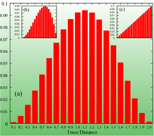
Figure 1: (color online) Probability distribution for the different values of trace distance ($d_{tr}(\rho,\zeta)=||\vec{r}-\vec{z}||_{2}$, where $\zeta=2^{-1}(\mathbb{I}_{2}+\vec{z}\cdot\vec{\sigma})$) for $10^{8}$ pairs of randomly-generated one-qubit states: (a) two density operators $(\rho\mbox{, }\zeta)$, (b) one mixed and one pure state $(\rho\mbox{, }|\zeta\rangle)$, and (c) two state vectors $(|\rho\rangle\mbox{, }|\zeta\rangle)$. The mean value of TD in the three cases are, respectively, $1.03$, $1.20$, and $1.33$.

It is worthwhile mentioning at this point that we have made several tests from which we found that the numerical and analytical results for the TD coincide up to the fifteenth digit when applied to random states in those classes considered in Secs. 2.2.1 and 2.1. More specifically, we generated one million pairs of random collinear states ($d=2$) and one million pairs of random pure states (see e.g. Ref. Maziero_pRPV ) for each value of the system dimension (with $d=2,\cdots,20$). The error, in each case, is computed by comparing the trace distance obtained via diagonalization with the LAPACK subroutines and the value of TD obtained using its analytical expression. Then the precision is established via the worst case error.

States generated	Percentage	$\langle G\rangle$	$\Delta G$	$G_{\mathrm{max}}$
$(\rho,\zeta),(\xi,\eta)$	$7.28$	$0.161$	$0.083$	$0.475$
$(\rho,\zeta),(\xi,|\eta\rangle)$	$7.86$	$0.186$	$0.091$	$0.486$
$(\rho,|\zeta\rangle),(\xi,|\eta\rangle)$	$3.16$	$0.071$	$0.038$	$0.190$
$(\rho,\zeta),(|\xi\rangle,|\eta\rangle)$	$4.06$	$0.134$	$0.072$	$0.333$
$(\rho,|\zeta\rangle),(|\xi\rangle,|\eta\rangle)$	$3.00$	$0.083$	$0.044$	$0.194$
$(\rho,\zeta),(\xi,\mathbb{I}_{2}/2)$	$8.49$	$0.192$	$0.098$	$0.488$
$(\rho,\zeta),(|\xi\rangle,\mathbb{I}_{2}/2)$	$20.75$	$0.226$	$0.096$	$0.500$
$(\rho,|\zeta\rangle),(\xi,\mathbb{I}_{2}/2)$	$3.20$	$0.101$	$0.045$	$0.248$
$(\rho,|\zeta\rangle),(|\xi\rangle,\mathbb{I}_{2}/2)$	$7.67$	$0.123$	$0.037$	$0.177$
$(|\rho\rangle,|\zeta\rangle),(\xi,\mathbb{I}_{2}/2)$	$2.63$	$0.107$	$0.043$	$0.177$
$(|\rho\rangle,|\zeta\rangle),(|\xi\rangle,\mathbb{I}_{2}/2)$	$8.85$	$0.169$	$0.004$	$0.177$

Table 1: Percentage of the $10^{6}$ quartets of randomly-generated one-qubit states leading to the NMuTP drawback of trace distance. In the last three columns are presented the average value, standard deviation, and maximum value of the strength of the NMuTP drawback of TD, as defined in Eq. (2.2.2), for each case study.

We proved in the previous subsections that if the pairs $(\rho,\zeta)$ and $(\xi,\eta)$ are, individually, collinear or if all the four states are pure, we shall have no NMuTP drawback of trace distance. However, as is shown in Table 1, for all the other possibilities a significant fraction of the one million one-qubit quartets of states randomly generated presented this unwanted property of TD. In Fig. 2 we draw an example of such a quartet of states.

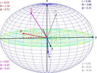
Figure 2: (color online) Example of a quartet of states for which the trace distance is not monotonic under taking tensor products of its arguments. Here $r$ is the size of the corresponding Bloch’s vector, the angles are given in radians, and $d_{tr}(\rho,\zeta)=0.80$, $d_{tr}(\xi,\eta)=0.76$, $d_{tr}(\rho^{\otimes 2},\zeta^{\otimes 2})=0.87$, and $d_{tr}(\xi^{\otimes 2},\eta^{\otimes 2})=1.07$.

For the sake of measuring the strength of the NMuTP drawback of TD, when applicable, we will define the following quantity:

$$G(\rho,\zeta,\xi,\eta) := |d_{tr}(\rho,\zeta)-d_{tr}(\xi,\eta)|$$

$$+|d_{tr}(\rho^{\otimes 2},\zeta^{\otimes 2})-d_{tr}(\xi^{\otimes 2},\eta^{\otimes 2})|.$$

The quantity $G$ measures how far the TD is from been monotonic under tensor products. As $G$ is defined only for those quartets of states leading to the NMuTP of TD, its lower bound is zero. In order to access more details about the distribution of $G$, we shall use its mean value $\langle G\rangle$, standard deviation $\Delta G$, and maximum value $G_{\mathrm{max}}$. These quantities are also shown in Table 1. A sample of the values of $G$ for the case study $(\rho,\zeta),(\xi,\eta)$ is presented in Fig. 3.

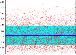
Figure 3: (color online) Values of the strength defined in Eq. (2.2.2) for one fourth of the $72802$ quartets of states leading to the NMuTP drawback of TD in the case study $(\rho,\zeta),(\xi,\eta)$, in one numerical experiment with one million random samples generated. The blue line is $\langle G\rangle$ and the points in the cyan area are values of $G$ in the interval $[\langle G\rangle-\Delta G,\langle G\rangle+\Delta G]$ (see Table 1).

Even with these additional informations, as can be seem in Table 1, in the general case the relationship between the existence of the NMuTP drawback of TD and the classes of states involved is not an easy matter. For instance, starting with general states and then restricting one of them to be pure we pass from a percentage of $7.28\mbox{ \%}$ to $7.86\mbox{ \%}$. But then the addition of the same restriction for one state of the other pair reduces the percentage with the undesired property of TD to $3.16\mbox{ \%}$. Several other similar nontrivial changes in the percentages can be identified. One striking one is that in the last line of the table. For four pure states there is no drawback, however just by putting one of the states in the center of the Bloch’s ball, we get a percentage of $8.85\mbox{ \%}$, the second higher among the classes of one-qubit states studied. These results stress the richness and complexity of the quantum state space, already for the composition of two of its simplest systems. Thus, in order to simplify the analysis, we will investigate in the next section the general dependence of the NMuTP drawback of TD with the dimension of the system.

2.3 General one-qudit states

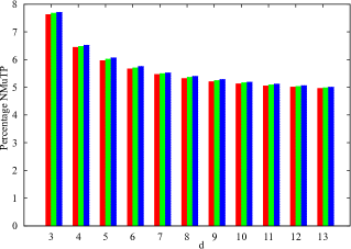
Figure 4: (color online) Minimum value (red bar on the left), mean value (green bar in the middle), and maximum value (blue bar on the right) of the fraction of the quartets of randomly-generated quantum states leading to the NMuTP drawback of trace distance as a function of the system’s dimension for ten numerical experiments. We generated one million quartets of states in each experiment.

In this subsection we shall study the NMuTP drawback of trace distance for $d-$level quantum systems, known as qudits. As there is no explicit parametrization for density matrices with $d\geq 3$ Petruccione_PofU , we will proceed as follows. Let us first look for the spectral decomposition of a given density operator $x=\rho\mbox{, }\zeta\mbox{, }\xi\mbox{, }\eta$:

$$x={\textstyle\sum_{j=1}^{d}x_{j}|x_{j}\rangle\langle x_{j}|}.$$ (15)

Once the eigenvalues of $x$ form a probability distribution, i.e.,

$$x_{j}\geq 0\mbox{ and }{\textstyle\sum_{j=1}^{d}x_{j}=1,}$$ (16)

we can use a geometric parametrization for them Fritzche4 :

$$x_{j}=\sin^{2}\theta_{j-1}{\textstyle\prod_{k=j}^{d-1}}\cos^{2}\theta_{k}$$ (17)

with $\theta_{0}=\pi/2$. The details about the numerical generation of $\{x_{j}\}$ using this parametrization can be found in Ref. Maziero_pRPV .

The basis formed by the eigenvectors of a density operator $x$, $\{|x_{j}\rangle\}$, can be obtained from the computational basis, $\{|j\rangle\}$, using an unitary matrix $U$, i.e.,

$$|x_{j}\rangle=U|j\rangle,\mbox{ with }j=1,\cdots,d.$$ (18)

There are several parametrizations for unitary matrices Petruccione_PofU . Here we use the Hurwitz’s parametrization with Euler’s angles. For details see e.g. Ref. Zyczkowski_U .

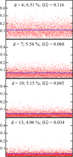
Figure 5: (color online) Samples with 5000 values of the strength of the NMuTP drawback of trace distance for some values of the system’s dimension $d$. The NMuTP average percentage of the whole sample with ten sets of $10^{6}$quartets of states is shown at the side of $d$. The blue line indicates $\langle G\rangle$.

By creating pseudo-random probability distributions $\{x_{j}\}$ and pseudo-random unitary matrices $U$, we did ten numerical experiments for each value of the system’s dimension $d$ generating one million quartets of states in each experiment. The mean, minimum, and maximum values of the percentages of the quartets of states leading to NMuTP of TD are shown in Fig. 4. In the Fig. 5 we present samples of the distribution of values of the drawback’s strength for some values of $d$. We can see in these figures a steady decreasing of such a proportion and strength as the system dimension $d$ grows.

3 Final remarks

The trace distance has several good properties that rank it as one of the major distance measures between quantum states. Nevertheless, it also presents a potential drawback, the possibility of being non-monotonic under taking tensor products of its arguments, that was shown in this article to exist for a non-negligible fraction of the density matrices investigated. Thus, although such issue seems not to be much relevant for high-dimensional quantum systems, it must be taken into account when dealing with few qubits.

The important question that yet remains is if, in the cases were the NMuTP of TD is significant, it has some undesirable consequence for important functions in quantum information science. The possible implications of this issue regarding, for instance, the quantification of quantum entanglement, of quantum discord, and of quantum coherence is an appealing topic for further researches. It would also be fruitful analyzing the NMuTP drawback considering other quantum distance measures. The obtention of a more precise operational and/or physical interpretation of $G$ and its upper bound are also left as open problems.

- (1) M.A. Nielsen and I.L. Chuang, Quantum Computation and Quantum Information (Cambridge University Press, Cambridge, 2000)
- (2) M.M. Wilde, Quantum Information Theory (Cambridge University Press, Cambridge, 2013)
- (3) C.A. Fuchs, Distinguishability and accessible information in quantum theory, arXiv:quant-ph/9601020
- (4) P. Neumann, N. Mizuochi, F. Rempp, P. Hemmer, H. Watanabe, S. Yamasaki, V. Jacques, T. Gaebel, F. Jelezko, J. Wrachtrup, Multipartite entanglement among single spins in diamond, Science 320, 1326 (2008)
- (5) P. Walther, K.J. Resch, T. Rudolph, E. Schenck, H. Weinfurter, V. Vedral, M. Aspelmeyer, and A. Zeilinger, Experimental one-way quantum computing, Nature 434, 169 (2005)
- (6) J. Zhang, R. Laflamme, and D. Suter, Experimental implementation of encoded logical qubit operations in a perfect quantum error correcting code, Phys. Rev. Lett. 109, 100503 (2012)
- (7) V. Scarani, S. Iblisdir, N. Gisin, and A. Acín, Quantum cloning, Rev. Mod. Phys. 77, 1225 (2005)
- (8) A.K. Pati, M.M. Wilde, A.R.U. Devi, A.K. Rajagopal, and Sudha, Quantum discord and classical correlation can tighten the uncertainty principle in the presence of quantum memor, Phys. Rev. A 86, 042105 (2012)
- (9) M. Zwolak, C.J. Riede, and W.H. Zurek, Amplification, redundancy, and quantum chernoff information, Phys. Rev. Lett. 112, 140406 (2014)
- (10) N. Boulant, T.F. Havel, M.A. Pravia, and D.G. Cory, Robust method for estimating the Lindblad operators of a dissipative quantum process from measurements of the density operator at multiple time points, Phys. Rev. A 67, 042322 (2003)
- (11) A. Gilchrist, N.K. Langford, and M.A. Nielsen, Distance measures to compare real and ideal quantum processes, Phys. Rev. A 71, 062310 (2005)
- (12) C.A. Fuchs and J. van de Graaf, Cryptographic distinguishability measures for quantum-mechanical states, IEEE Trans. Inf. Theory 45, 1216 (1999)
- (13) N. Gisin, G. Ribordy, W. Tittel, and H. Zbinden, Quantum cryptography, Rev. Mod. Phys. 74, 145 (2002)
- (14) S.-J. Gu, Fidelity approach to quantum phase transitions, Int. J. Mod. Phys. B 24, 4371 (2010)
- (15) A. Borrás, M. Casas, A.R. Plastino, and A. Plastino, Entanglement and the lower bounds on the speed of quantum evolution, Phys. Rev. A 74, 022326 (2006)
- (16) P.J. Jones and P. Kok, Geometric derivation of the quantum speed limit, Phys. Rev. A 82, 022107 (2010)
- (17) M.M. Taddei, B.M. Escher, L. Davidovich, and R.L. de Matos Filho, Quantum speed limit for physical processes, Phys. Rev. Lett. 110, 050402 (2013)
- (18) S. Deffner and E. Lutz, Quantum speed limit for non-Markovian dynamics, Phys. Rev. Lett. 111, 010402 (2013)
- (19) A. del Campo, I.L. Egusquiza, M.B. Plenio, and S.F. Huelga, Quantum speed limits in open system dynamics, Phys. Rev. Lett. 110, 050403 (2013)
- (20) Y.-J. Zhang, W. Han, Y.-J. Xia, J.-P. Cao, and H. Fan, Quantum speed limit for arbitrary initial states, Sci. Rep. 4, 4890 (2014)
- (21) F. Caruso, V. Giovannetti, C. Lupo, and S. Mancini, Quantum channels and memory effects, Rev. Mod. Phys. 86, 1203 (2014)
- (22) R. Horodecki, P. Horodecki, M. Horodecki, and K. Horodecki, Quantum entanglement, Rev. Mod. Phys. 81, 865 (2009)
- (23) L. Aolita, F. de Melo, and L. Davidovich, Open-system dynamics of entanglement: a key issues review, Rep. Prog. Phys. 78, 042001 (2015)
- (24) L.C. Céleri, J. Maziero, and R.M. Serra, Theoretical and experimental aspects of quantum discord and related measures, Int. J. Quant. Inf. 9, 1837 (2011)
- (25) K. Modi, A. Brodutch, H. Cable, T. Paterek, and V. Vedral, The classical-quantum boundary for correlations: Discord and related measures, Rev. Mod. Phys. 84, 1655 (2012)
- (26) A. Streltsov, Quantum Correlations Beyond Entanglement and Their Role in Quantum Information Theory (Springer, Berlin, 2015)
- (27) T. Baumgratz, M. Cramer, and M.B. Plenio, Quantifying coherence, Phys. Rev. Lett. 113, 140401 (2014)
- (28) J. Åberg, Catalytic coherence, Phys. Rev. Lett. 113, 150402 (2014)
- (29) D. Girolami, Observable measure of quantum coherence in finite dimensional systems, Phys. Rev. Lett. 113, 170401 (2014)
- (30) C.-s. Yu, Y. Zhang, and H. Zhao, Quantum correlation via quantum coherence, Quant. Inf. Process. 13, 1437 (2014)
- (31) K.M.R. Audenaert, Comparisons between quantum state distinguishability measures, Quant. Inf. Comp. 14, 31 (2014)
- (32) D. Bures, An extension of Kakutani’s theorem on infinite product measures to the tensor product of semifinite algebras, Trans. Amer. Math. Soc. 135, 199 (1969)
- (33) A. Uhlmann, The “transition probability” in the state space of a algebra, Rep. Math. Phys. 9, 273 (1976)
- (34) M. Bina, A. Mandarino, S. Olivares, and M.G.A. Paris, Drawbacks of the use of fidelity to assess quantum resources, Phys. Rev. A 89, 012305 (2014)
- (35) D. Pérez-García, M.M. Wolf, D. Petz, and M.B. Ruskai, Contractivity of positive and trace-preserving maps under Lp norms, J. Math. Phys. 47, 083506 (2006)
- (36) F.M. Paula, T.R. de Oliveira, and M.S. Sarandy, Geometric quantum discord through the Schatten 1-norm, Phys. Rev. A 87, 064101 (2013)
- (37) F.M. Paula, I.A. Silva, J.D. Montealegre, A.M. Souza, E.R. deAzevedo, R.S. Sarthour, A. Saguia, I.S. Oliveira, D.O. Soares-Pinto, G. Adesso, and M.S. Sarandy, Observation of environment-induced double sudden transitions in geometric quantum correlations, Phys. Rev. Lett. 111, 250401 (2013)
- (38) B. Dakić, V. Vedral, and Č. Brukner, Necessary and sufficient condition for nonzero quantum discord, Phys. Rev. Lett. 105, 190502 (2010)
- (39) H. Umegaki, Conditional expectation in an operator algebra. IV. Entropy and information, Kodai Math. Sem. Rep. 14, 59 (1962)
- (40) F. Hiai and D. Petz, The proper formula for relative entropy and its asymptotics in quantum probability, Comm. Math. Phys. 143, 99 (1991)
- (41) V. Vedral, The role of relative entropy in quantum information theory, Rev. Mod. Phys. 74, 197 (2002)
- (42) J. Maziero, Distribution of mutual information in multipartite states, Braz. J. Phys. 44, 194 (2014)
- (43) M. Nussbaum and A. Szkoła, The Chernoff lower bound for symmetric quantum hypothesis testing, Ann. Stat. 37, 1040 (2009)
- (44) K.M.R. Audenaert, J. Calsamiglia, R. Munõz-Tapia, E. Bagan, Ll. Masanes, A. Acin, and F. Verstraete, Discriminating states: The quantum Chernoff bound, Phys. Rev. Lett. 98, 160501 (2007)
- (45) E. Anderson, Z. Bai, C. Bischof, S. Blackford, J. Demmel, J. Dongarra, J. Du Croz, A. Greenbaum, S. Hammarling, A. McKenney, and D. Sorensen, LAPACK Users’ Guide, 3rd Ed. (Society for Industrial and Applied Mathematics, Philadelphia, 1999)
- (46) U. Fano, Pairs of two-level systems, Rev. Mod. Phys. 55, 855 (1983)
- (47) E. Brüning, H. Mäkelä, A. Messina, and F. Petruccione, Parametrizations of density matrices, J. Mod. Opt. 59, 1 (2012)
- (48) M. Matsumoto and T. Nishimura, Mersenne Twister: A 623-dimensionally equidistributed uniform pseudorandom number generator, ACM Trans. Model. Comput. Sim. 8, 3 (1998)
- (49) J. Maziero, Generating pseudo-random discrete probability distributions, Braz. J. Phys. 45, 377 (2015)
- (50) T. Radtke and S. Fritzsche, Simulation of n-qubit quantum systems. IV. Parametrizations of quantum states, matrices and probability distributions, Comput. Phys. Comm. 179, 647 (2008)
- (51) K. Życzkowski and M. Kuś, Random unitary matrices, J. Phys. A: Math. Gen. 27, 4235 (1994)