The Effect of Orbital Angular Momentum on Nondiffracting Ultrashort Optical Pulses

Abstract

We introduce a new class of nondiffracting optical pulses possessing orbital angular momentum. By generalizing the X-waves solution of the Maxwell equation, we discover the coupling between angular momentum and the temporal degrees of freedom of ultra-short pulses. The spatial twist of propagation invariant light pulse turns out to be directly related to the number of optical cycles. Our results may trigger the development on novel multi-level classical and quantum transmission channels free of dispersion and diffraction, may also find application in the manipulation of nano-structured objects by ultra-short pulses, and for novel approaches to the spatio-temporal measurements in ultrafast photonics.

Since the development of the laser, and in particular of mode locking modeL and Q-switching Qsw techniques, optical pulses have attracted a lot of interest, and their development influenced many fields of fundamental and applied research such as atomic physics, spectroscopy, communications, material processing and medicine, to name a few OP1 ; OP2 . As they are essentially suitable superpositions of plane waves that travel with different frequencies, optical pulses tend to diffract in both space and time during propagation. This feature constitutes a limiting factor for some applications like lithography lito , where the spatial broadening affects the quality of the generated mask, or communication science, where temporal broadening can induce additional noise between adjacent channels agrawal . To solve these issues, so-called localized waves localizedWaves , i.e., nondiffracting electromagnetic fields in both space and time, have been proposed in the last decades, with their most famous representatives being the X-waves. First introduced in acustics ref3 ; ref4 , X-waves were subsequently studied in different areas of physics, such as nonlinear optics ref5 ; ref6 , Bose-Einstein condensates ref7 , quantum optics ref8 and waveguide arrays ref8bis1 ; ref8bis , to name a few. Recently, they have also been proposed as a possible solution to efficient free space communication freeSpace .

X-waves are polychromatic superpositions of Bessel waves, and the related vast literature mostly considers superpositions of Bessel beams of order zero, and neglects their possible orbital angular momentum (OAM) content OAMX . OAM is indeed related to the twisted wavefront of higher order Bessel beam solutions of the Maxwell equations libroOAM . Seemingly, despite some published papers pulseAM1 ; pulseAM2 , OAM is still seldomly associated to ultrashort pulses, and only very recently some experimental results reported femtosecond vortex beams pulseOAM1 ; pulseOAM2 and Laguerre-Gauss supercontinuum pulseOAM3 .

The fact that light possesses both linear and angular momentum is known since the pioneering works by Poynting poynting and Darwin darwin . However, it is only thanks to the seminal works of Berry and Nye in 1974 berry and Allen and Woerdman in 1992 allenWoerdman that the OAM concept was brought into the field of optical beams, where it has been extensively studied both from a fundamental sep1 ; sep2 ; sep3 ; sep4 and experimental point of view, leading to striking applications such as optical tweezers tweezer and spanners spanner . Very recently, OAM has also been proposed as a new degree of freedom for encoding information in a superdense manner, and both its classical refCoding1 and quantum refCoding2 features have been investigated.

A challenging issue at the moment is generating ultrashort pulses with variable OAM; this would open unprecedented possibilities in terms of lightwave transmission systems unaffected by dispersion and diffractions. In this terms, a very prosiming direction is combining the non-diffracting character of X-waves with the superdense coding by OAM. Moreover, the extension of the concept of OAM to the domain of ultra-short optical pulses may give new insights on light-matter interaction, as recent works suggest vortexIon .

Following the recent experimental realization of higher order Bessel beams by holographic techniques BesselHigh , in this Letter we propose a new class of OAM-carrying non diffracting pulses. We consider superpositions of $m$-th order Bessel beams with an exponentially decaying spectrum, and generalize the well known fundamental X-waves localizedWaves . This new class of few-cycles optical pulses is not only an exact model for the connection between OAM and the ultra-fast photonics, but they are a new tool for OAM-based free-space quantum and classical communications by localized waves.

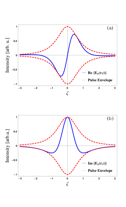
Figure 1: Real (a) and imaginary (b) part of the electric field component $E_{x}(\mathbf{r},t)$ as a function of the co-moving coordinate $\zeta=(z/c)\cos\vartheta_{0}-t$, for the case $m=1$. The real part is an odd function that crosses the line $\zeta=0$ three times, while the imaginary part is an even function, with two crossings. Parameters: $\vartheta_{0}=0.01$ (corresponding to the paraxial case) and $\alpha=1$; $\zeta$ is dimensionless.

We first introduce the general solution for X-waves with OAM. We start from a Bessel beam durnin , namely:

$$\psi(R,\theta,z)=\text{J}_{m}\left(\frac{\omega}{c}\sin\vartheta_{0}R\right)e^{im\theta}e^{i\omega z\cos\vartheta_{0}},$$ (1)

where $\omega=ck$ and $\vartheta_{0}$ is the Bessel cone angle, i.e., the beam’s characteristic parameter. Bessel beams carry OAM because they are eigenstates of the $z$-components of the angular momentum operator $\hat{L}_{z}=-i\partial/\partial\theta$ with eigenvalue $m$ AMQM . It is well known that Eq. (1) well describes a monochromatic field. It is not difficult, however, to generalize this result to the non-monochromatic case, where, following Ref. localizedWaves , the scalar field

$$\phi(\mathbf{r},t)=e^{im\theta}\int d\omega\;f(\omega)\text{J}_{m}\left(\frac{\omega}{c}\sin\vartheta_{0}R\right)e^{-i\omega(t-\frac{z}{c}\cos\vartheta_{0})},$$ (2)

is an exact solution of the full wave equation, being $f(\omega)$ an arbitrary spectrum. Equation (2) is known in literature to describe localized waves, namely field configurations that are well localized both in space and time. If the following exponentially decaying spectrum is used

$$f(\omega)=\omega^{n}e^{-\alpha\omega}\Theta(\omega),$$ (3)

where $\alpha$ is a parameter with the dimensions of a time that controls the width of the spectrum and $\Theta(\omega)$ is the Heaviside step function nist , Eq. (2) with $m=0$ describes the well known fundamental X-waves localizedWaves . For $m\neq 0$, however, Eq. (2) admits the following analytical solution gradstein :

$$\phi_{m}(\mathbf{r},t)=\frac{C_{n,m}\xi^{m}e^{im\theta}}{(\alpha+i\zeta)^{n+1}}\,_{2}F_{1}\left(a,b;m+1;-\xi^{2}\right),$$ (4)

where $C_{n,m}=(n+m)!/(2^{m}m!)$, $a=(n+m+1)/2$, $b=(n+m+2)/2$, $\xi=R\sin\vartheta_{0}/[c(\alpha+i\zeta)]$, $\zeta=(z/c)\cos\vartheta_{0}-t$ is the co-moving reference frame attached to the X-wave and $\,{}_{2}F_{1}(a,b;c,z)$ is the Gauss hypergeometric function nist . Eq. (4) represents a scalar X wave carrying $m$ units of OAM. Moreover, as ultrashort pulses are often modeled through an exponentially decaying spectrum OP1 , Eq. (4) can be therefore taken as a scalar ultrashort non diffracting wave that carries OAM. To correctly describe an optical ultrashort pulse, however, the scalar theory is no longer sufficient, and a full vector theory is required. An exact vectorial solution of Maxwell’s equation can be built from a scalar function by means of the so-called Hertz vector potentials stratton . We choose $\boldsymbol{\Pi}(\mathbf{r},t)=\hat{\mathbf{z}}\;\phi_{m}(\mathbf{r},t)$ as the Hertz potential, and the electric and magnetic vector fields are given by stratton :

$$\mathbf{E}(\mathbf{r},t) =\nabla\times\nabla\times\boldsymbol{\Pi}(\mathbf{r},t),$$ (5a)

$$\mathbf{B}(\mathbf{r},t) =\frac{\partial}{\partial t}\left[\nabla\times\boldsymbol{\Pi}(\mathbf{r},t)\right].$$ (5b)

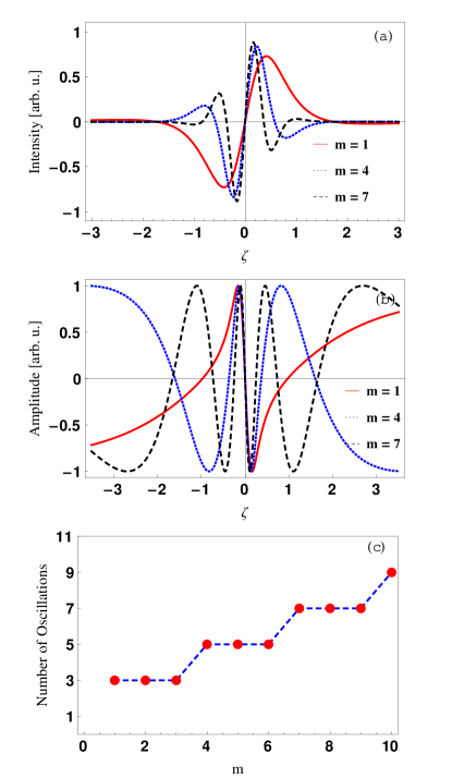
Figure 2: (a) Real part of the $x$-component of the electric field $E_{x}(\mathbf{r},t)$ for different values of the OAM parameter $m$. (b) Oscillatory function $\cos\psi(\mathbf{r},\zeta)$ for different values of the OAM parameter. The choice of these values corresponds to $\omega_{c}=3/\alpha$, $\omega_{c}=6/\alpha=2(\omega_{c})|_{m=1}$ and $\omega_{c}=9/\alpha=3(\omega_{c})|_{m=1}$, respectively. When the OAM increases, the carrier frequency blue shifts, with an increase of the number of optical cycles, but the envelope FWHM decreases, thus resulting in a shorter pulse. (c) Calculated (red dots) number of oscillations performed by $\cos\psi(\mathbf{r},\zeta)$ as a function of $m$. Every three units of $m$ added, the number of cycles of $\cos\psi(\mathbf{r},\zeta)$ grows by one unity. The number of oscillations is calculated by counting the number of zero crossing $N_{0}$ of each cosine term and using $N_{0}=2N_{osc}+1$. Here, $\vartheta_{0}=0.01$ (corresponding to the paraxial case) and $\alpha=1$ has been chosen. In particular, $\alpha=1$ means that $\zeta$ is a dimensionless quantity.

The explicit expression of the vector electric and magnetic fields generated with the above equations are available in the Supplementary Material. The real and imaginary parts of the $x$-component of the electric field $E_{x}(\mathbf{r},t)$ are depicted in Fig. 1 as a function of the co-moving coordinate $\zeta$. As can be seen, the real part is an odd function that crosses the axis $\zeta=0$ three times, while the imaginary part of the field is an even function, with only two crossings. This corresponds to a single-cycle optical-pulses following the definition in Ref. singleCycle . Note, moreover, that single-cycle optical-pulses are often described using of the so-called Ziolkowski’s modified power spectrum solution ziolkowski as generating scalar function. Here, instead, we have used fundamental X-waves with OAM to generate a new class of diffractionless single cycled optical pulses that naturally carry OAM. This is the first result of this Letter: Eq. (4) and its vector counterpart, defined through Eqs. (5), represent a new class of optical pulses, namely fundamental X-waves with OAM. With this result we can investigate the effects of OAM on optical pulses.

We consider, in particular, the case $m=1$, i.e., we assume to have a single-cycled optical pulse with one unit of OAM, and we study the connection between OAM and its temporal properties. We focus our attention on the $E_{x}(\mathbf{r},t)$ component; a similar discussion also holds for the other components. Fig. 2(a) shows the real part of the field for various values of the OAM parameter $m$. As can be seen, OAM affects the pulse’s temporal properties by changing its carrier frequency.

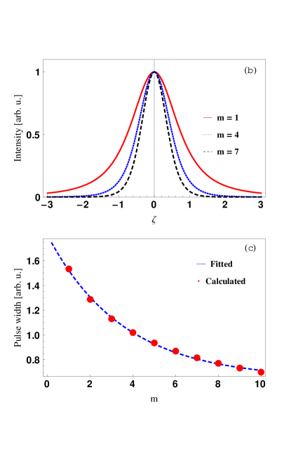
Figure 3: (a) Pulse envelope of the $x$-component of the electric field $E_{x}(\mathbf{r},t)$ for different values of the OAM parameter $m$. (b) Calculated (red dots) and fitted (blue dashed line) pulse width $\Delta\tau$ as a function of the OAM $m$. The fit predicts an exponential shortening of the pulse width with respect to $m$, according to $Ae^{-Bm}+C$. We have $A=1.16$, $B=0.28$ and $C=0.64$. Here, $\vartheta_{0}=0.01$ (corresponding to the paraxial case) and $\alpha=1$ has been chosen. In particular, $\alpha=1$ means that $\zeta$ is a dimensionless quantity.

As $m$ grows, in fact, the pulse’s carrier frequency $\omega_{c}$ also increases. Correspondigly, the field oscillates more rapidly, and the number of the optical cycles changes. To estabilish the relation between the carrier frequency $\omega_{c}$ and the OAM parameter $m$, we recall that an optical pulse is written as the product of an envelope function $A(\mathbf{r},t)$ and an harmonic term, i.e., $A(\mathbf{r},t)\exp{(-i\omega_{c}t)}$. As detailed in the supplementary material, for a general field, the carrier frequency can be calculated as the derivative of the phase $\psi$ of the field in $t=0$. Here, $\psi(\mathbf{r},t)=\arg[E_{x}(\mathbf{r},t)]$ and we obtain:

$$\omega_{c}=\left|\frac{\partial\psi(\mathbf{r},\zeta)}{\partial\zeta}\right|_{\zeta=0}=\frac{m+2}{\alpha},$$ (6)

where $\alpha$ is the spectral width of the pulse and the derivative has been taken with respect to the co-moving coordinate $\zeta$. It is worth noticing that the result of Eq. (6) is exact only in the paraxial regime, where $\vartheta_{0}\ll 1$. However, although for the nonparaxial case the expression of $\omega_{c}$ is much more complicated, it can be demonstrated that the variation of $\omega_{c}$ with $m$ can still be well described by a slightly modified version of Eq. (6), namely $\omega_{c}=(m+2)/\alpha+\sigma_{m}$, where $\sigma_{m}$ accounts for the nonparaxial corrections. Although $\sigma_{m}$ actually depends on $m$, this dependence is very weak, and it can be treated, at the leading order in $m$, like a constant shift. Eq. (6) is therefore valid independently of the value of $\vartheta_{0}$.

Fig. 2(b) shows the oscillatory term $\cos\psi(\mathbf{r},\zeta)$ (which, apart from an unimportant multiplicative factor, represents the real part of the field $E_{x}(\mathbf{r},t)$ note ) for various values of the OAM parameter $m$). This term increases by one optical cycle every three units of OAM. This result can be interpreted in a simple intuitive way: as the amount of OAM carried by the pulse grows, the pulse itself adapts to it by increasing the number of optical cycles that it is able to perform under its envelope.

The additional effect of OAM on the pulse is reported in Fig. 3(a), where the envelope of the field is plotted for various values of the OAM parameter $m$ . As the amount of OAM increases, the pulse duration given by its full-width half-maximum (FWHM) $\Delta\tau$, becomes smaller. To quantify this OAM-driven compression, we have numerically estimated $\Delta\tau$ for various $m$, and we show the results in Fig. 3 (b): $\Delta\tau$ decreases exponentially with $m$. This is the second result of our Letter. The amount of OAM carried by a nondiffracting optical pulse affects its temporal properties, namely it varies its time duration $\Delta\tau$ (making it smaller as $m$ increases) and also changes its carrier frequency in such a way that the pulse gains an extra optical cycle every three units of OAM it carries (after the first one). In other words, in order to have high values of OAM in propagation-invariant pulses one needs to resort to higher frequencies and shorter temporal duration. At a fixed carrier frequency the maximal angular momentum is given by Eq. (6).

In conclusion we have introduced a new class of optical pulses possessing OAM by generalizing the well-known fundamental X-waves. We have theoretically investigated the effects of OAM onto such pulses and shown that, as the amount of OAM carried by the pulse increases, the pulse’s carrier frequency increases accordingly, thus resulting in a shortening of the pulse width and the appearance (at certain discrete threshold of OAM) of extra field oscillations. Given the enormous interest that OAM has generated in the past years, we believe that its extension to the domain of optical pulses presented here with OAM-carrying X-waves will open the way for new and intriguing applications. In particular, this result sets a fundamental limit to the amount of OAM that a non diffracting optical pulse can carry. This could have interesting consequences for the case of superdense free space communication protocols with X-waves.

The authors thank the German Ministry of Education and Science (ZIK 03Z1HN31) for financial support.

References

- (1) W. E. Lamb Jr., Phys. Rev. 134, A1429 (1964).
- (2) F. J. McClung and R. W. Hellwarth, J. Appl. Phys. 33, 828 (1962).
- (3) A. Weiner, Ultrafast Optics, Wiley (2009).
- (4) F. X. Kärtner, Few-Cycle Laser Pulse Generation and Its Applications (Topics in Applied Physics), Spinrger (2010).
- (5) S. Okazaki, J. Vac. Sci. Technol. B 9, 2829 (1991).
- (6) G. P. Agrawal, Fiber optics Communication Systems, Wiley (2002).
- (7) H. E. Hernandez-Figueroa, M. Zamboni-Rached and E. recami (editors), Localized Waves, Wiley (2008).
- (8) J. Lu and J. F. Greenleaf, IEEE Trans. Ultrason. Ferroelectr. Freq. Control 39, 19 (1992).
- (9) J. Lu and J. F. Greenleaf, IEEE Trans. Ultrason. Ferroelectr. Freq. Control 39, 441 (1992).
- (10) C. Conti, S. Trillo, P. Di Trapani, G. Valiulis, A. Piskarskas, O. Jedrkiewicz and J. Trull, Phys. Rev. Lett. 90, 170406 (2003).
- (11) G. Valiulis, J. Kilius, O. Jedrkiewicz, A. Bramati, S. Minardi, C. Conti, S. Trillo, A. Piskarskas and P. Di Trapani in Quantum Electronics and Laser Science Conference, Vol. 57 of Trends in Optics and Photonics (Optical Society of America, 2001).
- (12) C. Conti and S. Trillo, Phys. Rev. Lett. 92, 120404 (2004).
- (13) A. Ciattoni and C. Conti, J. Opt. Soc. Am. B 24, 2195 (2007).
- (14) Y. Lahini, E. Frumker, Y. Silberberg, S. Droulias, K. Hizanidis, R. Morandotti and D. N. Christodoulides, Phys. Rev. Lett. 98, 023901 (2007).
- (15) M. Heinrich, A. Szameit, F. Dreisow, R. Keil, S. Minardi, T. Pertsch, S. Nolte, A. Tünnermann and F. Lederer, Phys. Rev. Lett. 103, 113903 (2009).
- (16) J. Lu and S. He, Opt. Commun 161, 187 (1999).
- (17) D. L. Andrews and M. Babiker (editors), The Angular Momentum of Light, Cambridge (2012).
- (18) M. A. Salem and H. Bagci, Opt. Express 19, 8526 (2011).
- (19) J. Lekner, J. Opt. A: Pure Appl. Opt. 5, L15 (2003).
- (20) J. Lekner, J. Opt. A: Pure Appl. Opt. 6, 146 (2004).
- (21) K. Bezuhanov, A. Dreischuh, G. G. Paulus, M. Schätzel and H. Walther, Opt. Lett 29, 1942 (2004).
- (22) I. G. Mariyenko, J. Strohaber and C. J. G. J Uiterwaal, Opt. Express 19, 7599 (2005).
- (23) H. I. Sztul, V. Kortazayev and R. R. Alfano, Opt. Lett. 31, 2725 (2006).
- (24) J. H. Poynting, Proc. R. Soc. Lond. A Ser. A 82, 560-567 (1909).
- (25) C. G. Darwin, Proc. R. Soc. Lond. A 136, 36-52 (1932).
- (26) J. F. Nye and M. V. Berry, Proc. R. Soc. Lond. Ser. A 336, 1605 (1974).
- (27) L. Allen, M. W. Beijersbergen, R. J. C. Spreeuw and J. P. Woerdman, Phys. Rev. A 45, 8185-8189 (1992).
- (28) S. J. van Enk, and G. Nienhuis, Europhys. Lett., 25, 497-501 (1994).
- (29) S. M. Barnett and L. Allen, Opt. Comm. 110, 670-678 (1994).
- (30) I. Bialynicki-Birula and Z. Bialynicki-Birula, J. Opt. 13, 064014 (2011).
- (31) M. Ornigotti and A. Aiello, Opt. Express 22, 6586 (2014).
- (32) S. Franke-Arnold , L. Allen and M. Padgett, Laser & Photon. Rev. 2, 299 (2008).
- (33) M. Padgett and R. Bowman, nat, Phot 5, 343 (2011).
- (34) J. Wang, J. Y. Yang, I. M. Fazal, N. Ahmed, Y. Yan, H. Huang, Y. Ren,Y. Yue, S. Dolinar, M. Tur and A. E. Willner, Nat. Phot. 6, 488 (2012).
- (35) R. Fickler, R. Lapkiewicz, W. N. Plick, M. Krenn, C. Schaeff, S. Ramelov and A. Zeilinger, Science 338, 640 (2012).
- (36) A. Picon, J. Mompart, J.R. Vazquez de Aldana, L. Plaja, G. F. Calvo and L. Roso, Opt. Express 18, 3660 (2010).
- (37) R. Vasilyeu, A. Dudley, and A. Forbes, Opt. Express 17, 23389 (2009).
- (38) J. Durnin, J. J. Miceli and J. H. Eberly, Phys. Rev. Lett 58 1499 (1987)
- (39) S. Feng, H. G. Winful and R. W. Hellwarth, Phys. Rev. E 59, 4630 (1999).
- (40) A. R. Edmonds, Angular Momentum in Quantum Mechanics, Princeton University Press (1996).
- (41) Digital Library of Mathematical Functions, http://dlmf.nist.gov, National Institute of Standard and Technology (2010).
- (42) I. S. Gradshteyn and I. M. Ryzhiz, Table of Integrals, Series and Products, Academic Press (2006).
- (43) J. A. Stratton, Electromagnetic Theory, Dover (2010).
- (44) R. W. Ziolkowski, J. Math. Phys. 26, 861 (1985).
- (45) In the complex exponential notation, the electric field can be written as , where . Then, the real part of this field can be written as . To analyze the frequency properties of this field, it is therefore enough to analyze only its oscillatory part, i.e., .