A NEW METHOD FOR NUMERICAL SOLUTION OF THE FRACTIONAL RELAXATION AND SUBDIFFUSION EQUATIONS USING FRACTIONAL TAYLOR POLYNOMIALS

Abstract

The accuracy of the numerical solution of a fractional differential equation depends on the differentiability class of the solution. The derivatives of the solutions of fractional differential equations often have a singularity at the initial point, which may result in a lower accuracy of the numerical solutions. We propose a method for improving the accuracy of the numerical solutions of the fractional relaxation and subdiffusion equations based on the fractional Taylor polynomials of the solution at the initial point.
AMS Subject Classification: 33F05, 34A08, 57R10
Key words: fractional differential equation, Caputo derivative, numerical solution, fractional Taylor polynomial.

1 Introduction

Differential equations with fractional derivatives are used for modeling non-Markovian processes in various areas of science such as Physics, Biology and Economics [1-5]. The methods for analytical solution of ordinary and partial fractional differential equations can be applied to only special types of equations and initial conditions. In practical applications the solutions of the fractional differential equations are determined by numerical methods. The development of efficient methods for numerical solution of fractional differential equations is an active research field.

An important approximation for the Caputo fractional derivative is the $L1$ approximation (3). It has been successfully used for numerical solution of ordinary and partial fractional differential equations. When the function $y(x)$ is a smooth function, the accuracy of the $L1$ approximation is $O\left(h^{2-\alpha}\right)$. In previous work [13] we determined the second order approximation (4) by modifying the first three coefficients of the $L1$ approximation with the value of the Riemann zeta function at the point $\alpha-1$, and we computed the numerical solutions of the fractional relaxation and subdiffusion equations with sufficiently differentiable solutions. The solutions of fractional differential equations often have a singularity at the initial point. In this case the numerical solutions may converge to the exact solution but their accuracy may be lower than the expected accuracy from the numerical analysis. In this paper we propose a method for improving the accuracy of the numerical solutions of the fractional relaxation equation

$$y^{(\alpha)}(x)+By(x)=0,\quad y(0)=1,$$ (1)

where $0<\alpha<1$, and the fractional subdiffusion equation

$$\left\{\begin{array}[]{l l}\dfrac{\partial^{\alpha}u(x,t)}{\partial t^{\alpha}}=\dfrac{\partial^{2}u(x,t)}{\partial x^{2}},\quad x\in[0,\pi],t>0,&\\ u(x,0)=\sin x,\;u(0,t)=0,\;u(\pi,t)=0.\end{array}\right.$$ (2)

When the solutions of the relaxation and subdiffusion equations are smooth functions the accuracy of the numerical solutions using the $L1$ approximation are $O\left(h^{2-\alpha}\right)$ and $O\left(\tau^{2-\alpha}+h^{2}\right)$ and the numerical solutions using the modified $L1$ approximation have accuracy $O\left(h^{2}\right)$ and $O\left(\tau^{2}+h^{2}\right)$. The solutions of the fractional relaxation and subdiffusion equations (1) and (2) have differentiable singularities at the initial point. The accuracy of the numerical solutions (10) and (11) of the fractional relaxation equation is $O\left(h^{\alpha}\right)$ and the numerical solutions (20) and (21) of the fractional subdiffusion equation have accuracy $O\left(\tau+h^{2}\right)$. Equations (1) and (2) are linear fractional differential equations. The form of the equations allows us to compute the Miller-Ross derivatives of the solutions at the initial point. In section 3 and section 4 we use the fractional Taylor polynomials to improve the differentiability properties of the solutions and the accuracy of the numerical methods.

The Caputo derivative of order $\alpha$, where $0<\alpha<1$ is defined as

$$D_{\_}C^{\alpha}y(x)=y^{(\alpha)}(x)=\dfrac{d^{\alpha}}{dx^{\alpha}}y(x)=\dfrac{1}{\Gamma(1-\alpha)}\int_{\_}0^{x}\dfrac{y^{\prime}(\xi)}{(x-\xi)^{\alpha}}d\xi.$$

When the function $y$ is defined on the interval $(-\infty,x]$, the lower limit of the integral in the definition of Caputo derivative is $-\infty$. The value of the fractional derivative $y^{(\alpha)}(x)$ depends on the values of the function on the whole interval of definition. One approach for discretizing the Caputo derivative is to divide the interval to subintervals of small length and approximate the derivative of the function $y(x)$ using spline interpolation or a Lagrange polynomial [17]. Let $h$ be a small positive number. Denote

$$x_{\_}n=nh,\;y_{\_}n=y(x_{\_}n)=y(nh).$$

The $L1$ approximation for Caputo derivative is derived [13] by approximating the derivative of the function $y(x)$ on the interval $\left[x_{\_}{k-1},x_{\_}k\right]$ with its value $y^{\prime}_{\_}{k-0.5}$ at the midpoint of the interval.

$$y^{(\alpha)}_{\_}n\approx\dfrac{1}{h^{\alpha}\Gamma(2-\alpha)}\sum_{\_}{k=0}^{n-1}\sigma_{\_}k^{(\alpha)}y_{\_}{n-k},$$ (3)

where $\sigma_{\_}0^{(\alpha)}=1,\;\sigma_{\_}n^{(\alpha)}=(n-1)^{1-\alpha}-n^{1-\alpha}$ and

$$\sigma_{\_}k^{(\alpha)}=(k+1)^{1-\alpha}-2k^{1-\alpha}+(k-1)^{1-\alpha},\quad(k=1,\cdots,n-1).$$

When the function $y(x)$ has a continuous second derivative, the accuracy of the $L1$ approximation is $O\left(h^{2-\alpha}\right)$ ([18]). The modified $L1$ approximation for the Caputo derivative

$$y^{(\alpha)}_{\_}n\approx\dfrac{1}{\Gamma(2-\alpha)h^{\alpha}}\sum_{\_}{k=0}^{n}\delta_{\_}k^{(\alpha)}y_{\_}{n-k},$$ (4)

has coefficients $\delta_{\_}k^{(\alpha)}=\sigma_{\_}k^{(\alpha)}$ for $2\leq k\leq n$,

$$\delta_{\_}0^{(\alpha)}=\sigma_{\_}0^{(\alpha)}-\zeta(\alpha-1),\delta_{\_}1^{(\alpha)}=\sigma_{\_}1^{(\alpha)}+2\zeta(\alpha-1),\delta_{\_}2^{(\alpha)}=\sigma_{\_}2^{(\alpha)}-\zeta(\alpha-1),$$

where $\zeta(x)$ is the Riemann zeta function. The modified $L1$ approximation has accuracy $O\left(h^{2}\right)$.

By approximating the Caputo derivative at the point $x_{\_}n$ with (3) and (4) we obtain the numerical solutions (10) and (11) of the fractional relaxation equation. In Table 1 and Table 2 we compute the maximum error and the order of the numerical solutions (10) and (11) for the following equations

$$y^{(0.5)}(x)+y(x)=x^{2}+\dfrac{8}{3\sqrt{\pi}}x^{1.5},\quad y(0)=0,$$ (5)

$$y^{(0.5)}(x)+y(x)=x^{1.25}+\dfrac{5\sqrt{2}}{24\pi}\Gamma^{2}(0.25)x^{0.75},\quad y(0)=0.$$ (6)

Equations (5) and (6) have solutions $y(t)=x^{2}$ and $y(t)=x^{1.25}$. The solution of equation (6) has an unbounded second derivative at $t=0$. While the numerical solutions of equation (6) converge to the exact solution, their accuracy is smaller than $O\left(h^{2-\alpha}\right)$.

Table 1: Maximum error and order of numerical solutions (10) and (11) for equation (5) on the interval $[0,1]$.

$h$	$Error$	$Order$
$0.05$	$0.00281532$	$1.45619$
$0.025$	$0.00101549$	$1.47112$
$0.0125$	$0.00036392$	$1.48049$
$0.00625$	$0.00012986$	$1.48661$
$0.003125$	$0.00004621$	$1.49072$

$h$	$Error$	$Order$
$0.05$	$0.000695507$	$1.90440$
$0.025$	$0.000182729$	$1.92836$
$0.0125$	$0.000047388$	$1.94711$
$0.00625$	$0.000012168$	$1.96139$
$0.003125$	$3.10\times 10^{-6}$	$1.97206$

Table 2: Maximum error and order of numerical solutions (10) and (11) for equation (6) on the interval $[0,1]$.

$h$	$Error$	$Order$
$0.05$	$0.001825790$	$1.1544$
$0.025$	$0.000806728$	$1.17836$
$0.0125$	$0.000357787$	$1.17298$
$0.00625$	$0.000156707$	$1.19103$
$0.003125$	$0.000067873$	$1.20717$

$h$	$Error$	$Order$
$0.05$	$0.001825790$	$1.15440$
$0.025$	$0.000806728$	$1.17836$
$0.0125$	$0.000351853$	$1.19711$
$0.00625$	$0.000151948$	$1.21139$
$0.003125$	$0.000065135$	$1.22206$

The fractional relaxation equation (1) and the fractional subdiffusion equation (2) have solutions

$$y(x)=E_{\_}\alpha\left(-Bx^{\alpha}\right),\quad u(x,t)=\sin xE_{\_}\alpha\left(-t^{\alpha}\right).$$

Both solutions have a differentiable singularity at the initial point of fractional differentiation. Jin, Lazarov and Zhou [16] discuss the numerical solution of the fractional subdiffusion equation with accuracy in the time direction $O(\tau)$ and determine that the accuracy of the numerical solution (10) of the relaxation equation (1) is $O\left(h^{\alpha}\right)$. Murillo and Yuste [22] use a finite difference method with adaptive non-uniform timesteps for numerical solution of the fractional subdiffusion and diffusion-wave equations. In section 3 and section 4 we present a method for improving the accuracy of the numerical solutions of equations (1) and (2) based on the fractional Taylor polynomials of the solution.

2 Preliminaries

The values of a differentiable function close to the point $x=x_{\_}0$ are approximated by its Taylor polynomials of degree $m$

$$y(x)\approx\sum_{\_}{n=0}^{m}\dfrac{(x-x_{\_}0)^{n}}{n!}y^{(n)}(x_{\_}0).$$

The definition of fractional Taylor polynomials at the point $x=0$ is based on the composition of Caputo derivatives. The Miller-Ross sequential fractional derivative for the Caputo derivative is defined as

$$D^{\alpha_{\_}1}y(x)=D_{\_}C^{\alpha_{\_}1}y(x),\quad D^{\alpha_{\_}1+\alpha_{\_}2}y(x)=D_{\_}C^{\alpha_{\_}1}D_{\_}C^{\alpha_{\_}2}y(x),$$

and

$$D^{\alpha_{\_}1+\alpha_{\_}2+\cdots+\alpha_{\_}n}y(x)=D_{\_}C^{\alpha_{\_}1}D_{\_}C^{\alpha_{\_}2}\cdots D_{\_}C^{\alpha_{\_}n}y(x).$$

When $y(x)$ is a differentiable function

$$D^{0.5+0.5}y(x)=D_{\_}C^{0.5}y(x)D_{\_}C^{0.5}y(x)=D_{\_}C^{1}y(x)=y^{\prime}(x).$$

The Caputo derivative $D_{\_}C^{1}y(x)=y^{\prime}(x)$ and the Miller-Ross derivative $D^{0.5+0.5}y(x)$ of the function $y(x)=1+x^{0.5}+x$ are different.

$$D_{\_}C^{1}y(x)=y^{\prime}(x)=1+0.5x^{-0.5},$$

$$D^{0.5+0.5}y(x)=D_{\_}C^{0.5}D_{\_}C^{0.5}y(x)=D_{\_}C^{0.5}\left(\Gamma(1.5)+\dfrac{1}{\Gamma(1.5)}x^{0.5}\right)=1.$$

Two important functions in Fractional Calculus are the Mittag-Leffler and the Gamma function

$$\Gamma(x)=\int_{\_}0^{\infty}e^{-\xi}\xi^{x-1}d\xi.$$

The Gamma function has values $\Gamma(0)=\Gamma(1)=1,\Gamma(0.5)=\sqrt{\pi}$ and satisfies

$$\Gamma(1+x)=x\Gamma(x),\quad\Gamma(x)\Gamma(1-x)=\dfrac{\pi}{\sin\pi x}.$$

The one-parameter and two-parameter Mittag-Leffler functions are defined for $\alpha>0$ as

$$E_{\_}\alpha(x)=\sum_{\_}{n=0}^{\infty}\dfrac{x^{n}}{\Gamma(\alpha n+1)},\quad E_{\_}{\alpha,\beta}(x)=\sum_{\_}{n=0}^{\infty}\dfrac{x^{n}}{\Gamma(\alpha n+\beta)}.$$

When $\alpha=\beta=1$ the Mittag-Leffler functions are equal to the exponential function. The Mittag-Leffler functions appear in the solutions of fractional differential equations. The Laplace transform of the derivatives of the Mittag-Leffler functions satisfy

$$\mathcal{L}\{x^{\alpha k+\beta-1}E^{(k)}_{\_}{\alpha,\beta}(\pm ax^{\alpha})\}(s)=\dfrac{k!s^{\alpha-\beta}}{\left(s^{\alpha}\mp a\right)^{k+1}}.$$

The next theorem is a generalization of the Mean-Value Theorem for differentiable functions.

Theorem.

(Generalized Mean-Value Theorem)

$$y(x)=y(0)+\dfrac{x^{\alpha}}{\Gamma(\alpha+1)}y^{(\alpha)}(\xi_{\_}x)\quad(0\leq\xi_{\_}x\leq x).$$

In this paper we denote

$$D^{n\alpha}y(x)=D^{\alpha+\alpha+\cdots+\alpha}y(x)=D_{\_}C^{\alpha}D_{\_}C^{\alpha}\cdots D_{\_}C^{\alpha}y(x).$$

When the function $y(x)$ has nonzero Miller-Ross derivatives $D^{n\alpha}y(0)$ the value of $y(h)$ is approximated by the fractional Taylor polynomials [10].

$$y(h)\approx\sum_{\_}{n=0}^{m}\dfrac{h^{\alpha n}}{\Gamma(\alpha n+1)}D^{n\alpha}y(0),$$

where $h$ is a small positive number. The Miller-Ross derivatives of the function $E_{\_}\alpha\left(x^{\alpha}\right)$ satisfy

$$D^{n\alpha}E_{\_}\alpha\left(x^{\alpha}\right)=E_{\_}\alpha\left(x^{\alpha}\right),\quad\left.D^{n\alpha}E_{\_}\alpha\left(x^{\alpha}\right)\right|_{\_}{x=0}=E_{\_}\alpha\left(0\right)=1.$$

The integer order derivatives of the function $E_{\_}\alpha\left(x^{\alpha}\right)\rightarrow\pm\infty$ as $x\rightarrow 0$. When $h$ is a small number, the value of $E_{\_}\alpha\left(h^{\alpha}\right)$ is approximated by its fractional Taylor polynomials.

The fractional relaxation and subdiffusion equations,

$$y^{(0.5)}(x)+y(x)=0,\quad y(0)=1,$$ (7)

$$\left\{\begin{array}[]{l l}\dfrac{\partial^{0.5}u(x,t)}{\partial t^{0.5}}=\dfrac{\partial^{2}u(x,t)}{\partial x^{2}},&\\ u(x,0)=\sin x,\;u(0,t)=u(\pi,t)=0,&\\ \end{array}\right.$$ (8)

have solutions $y(x)=E_{\_}{0.5}\left(-x^{0.5}\right)$ and $u(x,t)=\sin xE_{\_}{0.5}\left(-t^{0.5}\right)$.

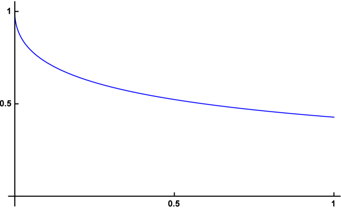
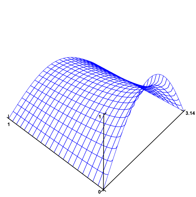
Figure 1: Graphs of the solutions of the fractional relaxation and subdiffusion equations (7) and (8).

In [13] we determined the finite-difference approximations (20) and (21) for the fractional subdiffusion equation. The second derivative in the space direction is approximated by second order central difference. Numerical solution (20) uses the $L1$ approximation for the Caputo derivative in the time direction and (21) uses the modified $L1$ approximation. In Table 3 and Table 4 we compute the maximal error and the order of numerical solutions (10) and (11) of the fractional relaxation equation (7) on the interval $[0,1]$, and the numerical solutions (20) and (21) of the subdiffusion equation (8) on the rectangle $[0,1]\times[0,\pi]$.

Table 3: Maximum error and order of numerical solutions (10) and (20) of the relaxation equation (7) on $[0,1]$ (left) and the subdiffusion equation (8) when $\tau=3h/\pi$, at time $t=1$ (right).

$h$	$Error$	$Order$
$0.05$	$0.0442319$	$0.378959$
$0.025$	$0.0331978$	$0.414001$
$0.0125$	$0.024484$	$0.439247$
$0.00625$	$0.0178342$	$0.457192$
$0.003125$	$0.0128769$	$0.469859$

$\tau\;(h=\pi\tau/3)$	$Error$	$Order$
$0.05\quad$	$0.00382782$	$1.08802$
$0.025\quad$	$0.00184202$	$1.05524$
$0.0125\quad$	$0.00089863$	$1.03549$
$0.00625\quad$	$0.00044211$	$1.02333$
$0.003125\quad$	$0.00021867$	$1.01563$

Table 4: Maximum error and order of numerical solutions (11) and (21) of the relaxation equation (7) on $[0,1]$ (left) and the subdiffusion equation (8) when $\tau=3h/\pi$, at time $t=1$ (right).

$h$	$Error$	$Order$
$0.05$	$0.0442319$	$0.378959$
$0.025$	$0.0331978$	$0.414001$
$0.0125$	$0.024484$	$0.439247$
$0.00625$	$0.0178342$	$0.457192$
$0.003125$	$0.0128769$	$0.469859$

$\tau\;(h=\pi\tau/3)$	$Error$	$Order$
$0.05\quad$	$0.00222875$	$1.03303$
$0.025\quad$	$0.00108596$	$1.03727$
$0.0125\quad$	$0.00053127$	$1.03146$
$0.00625\quad$	$0.00026116$	$1.02448$
$0.003125\quad$	$0.00012893$	$1.01838$

The accuracy of numerical solution (10) is $O\left(h^{\alpha}\right)$ ([16, Example 3.1]). The maximum error and order of numerical solutions (10) and (11) for the fractional relaxation equation (7) are given in Table 3 (left) and Table 4 (left). The two numerical solutions have the same maximal error. The maximum error is attained at the first approximation for $y(h)$. Both numerical solutions use the same approximation $v_{\_}1=w_{\_}1$ for $y(h)$. Now we show that the error of the approximation $v_{\_}1$ for $y(h)$ is $O\left(h^{0.5}\right)$.

$$y(h)=E_{\_}{0.5}\left(-h^{0.5}\right)=\sum_{\_}{n=0}^{\infty}\dfrac{\left(-h^{0.5}\right)^{n}}{\Gamma(0.5n+1)},$$

$$y(h)=1-\dfrac{2}{\sqrt{\pi}}h^{0.5}+O\left(h\right).$$

The approximation $v_{\_}1=w_{\_}1$ for $y(h)$ is computed with $v_{\_}0=1$ and

$$\dfrac{v_{\_}1-v_{\_}0}{\Gamma(1.5)h^{0.5}}+v_{\_}1=0,\quad v_{\_}1\left(1+\Gamma(1.5)h^{0.5}\right)-1=0,$$

$$v_{\_}1=\dfrac{1}{1+\Gamma(1.5)h^{0.5}}=1-\dfrac{\sqrt{\pi}}{2}h^{0.5}+O\left(h\right).$$

Then

$$\left|y(h)-v_{\_}1\right|=\left(\dfrac{\sqrt{\pi}}{2}-\dfrac{2}{\sqrt{\pi}}\right)h^{0.5}+O\left(h\right).$$

The accuracy of the approximation $v_{\_}1=w_{\_}1$ for $y(h)$ is $O\left(h^{0.5}\right)$.

3 Numerical Solutions of the Fractional Relaxation Equation

The fractional relaxation equation is an important ordinary fractional differential equation. The numerical and analytical solutions of the relaxation equation are discussed in [3,7,9,11-14]. The exact solution of the equation

$$y^{(\alpha)}(x)+By(x)=F(x),\;y(0)=1,$$ (9)

is determined with the Laplace transform method

$$y(x)=E_{\_}{\alpha}(-Bx^{\alpha})+\int_{\_}{0}^{x}\xi^{\alpha-1}E_{\_}{\alpha,\alpha}\left(-B\xi^{\alpha}\right)F(x-\xi)d\xi.$$

The numerical solutions $\left\{v_{\_}n\right\}$ and $\left\{w_{\_}n\right\}$ of the fractional relaxation equation (9) for approximations (3) and (4) are computed explicitly with $v_{\_}0=1$ ([13]),

$$v_{\_}n=\dfrac{1}{\sigma_{\_}0^{(\alpha)}+Bh^{\alpha}\Gamma(2-\alpha)}\left(\Gamma(2-\alpha)h^{\alpha}F_{\_}n-\sum_{\_}{k=1}^{n}\sigma_{\_}k^{(\alpha)}v_{\_}{n-k}\right),$$ (10)

and $w_{\_}0=1,w_{\_}1=v_{\_}1$,

$$w_{\_}n=\dfrac{1}{\delta_{\_}0^{(\alpha)}+Bh^{\alpha}\Gamma(2-\alpha)}\left(\Gamma(2-\alpha)h^{\alpha}F_{\_}n-\sum_{\_}{k=1}^{n}\delta_{\_}k^{(\alpha)}w_{\_}{n-k}\right).$$ (11)

When $F(x)=0$, the fractional relaxation equation

$$y^{(\alpha)}(x)+By(x)=0,\quad y(0)=1,$$

has the solution $y(x)=E_{\_}{\alpha}(-Bx^{\alpha})$. In section 2 we computed the numerical solutions (10) and (11) of equation (1) for $\alpha=0.5$. Both numerical solutions have maximum error at the first approximation $v_{\_}1=w_{\_}1$ and accuracy $O\left(h^{0.5}\right)$. The numerical experiments in this section confirm that the accuracy of $\eqref{NS1}$ and $\eqref{NS2}$ for equation $\eqref{R1}$ is $O\left(h^{\alpha}\right)$ when $\alpha=0.3$ and $\alpha=0.7$ and all values of $\alpha$ between $0$ and $1$. In this section we improve the accuracy of $\eqref{NS1}$ and $\eqref{NS2}$ using the fractional Taylor polynomials of the solution at the point $x=0$. The improved numerical solutions have accuracy $O\left(h^{2-\alpha}\right)$ and $O\left(h^{2}\right)$. In Fig. 2 we compare (10) with the improved numerical solution (14) and the exact solution of equation (1) for $\alpha=0.3$.

The fractional relaxation equation is a linear ordinary fractional differential equation. We can determine the Miller-Ross derivatives of the solution at $x=0$ using fractional differentiation. The Miller-Ross fractional derivative of order $\alpha$ is equal to the Caputo derivative. Write the relaxation equation in the form

$$D^{\alpha}y(x)+By(x)=0,\;y(0)=1.$$ (12)

When $x=0$ we obtain $D^{\alpha}y(0)=-By(0)=-B$. By applying fractional differentiation of order $\alpha$

$$D^{2\alpha}y(x)+BD^{\alpha}y(x)=0,$$

$$D^{3\alpha}y(x)+BD^{2\alpha}y(x)=0.$$

From the above equations we determine the values of $D^{2\alpha}y(0)$ and $D^{3\alpha}y(0)$.

$$D^{2\alpha}y(0)=-BD^{\alpha}y(0)=B^{2},\quad D^{3\alpha}y(0)=-BD^{2\alpha}y(0)=-B^{3}.$$

By differentiating $n-1$ times equation (12) we obtain

$$D^{n\alpha}y(0)=-BD^{(n-1)\alpha}y(0).$$

By induction we can show that $D^{n\alpha}y(0)=(-B)^{n}$. When $h$ is a small number, the fractional Taylor polynomials approximate the value of $y(h)$

$$y(h)\approx\sum_{\_}{n=0}^{m}\dfrac{\left(-Bh^{\alpha}\right)^{n}}{\Gamma(\alpha n+1)}.$$

Now we use the fractional Taylor polynomials for improving the differentiability properties of the solution of the relaxation equation. Let $m$ be a positive integer such that $m\alpha\geq 2$. Substitute

$$z(x)=y(x)-\sum_{\_}{n=0}^{m}\dfrac{\left(-Bx^{\alpha}\right)^{n}}{\Gamma(\alpha n+1)}.$$

The Caputo derivative of the function $z(x)$ is

$$z^{(\alpha)}(x)=y^{(\alpha)}(x)+B\sum_{\_}{n=0}^{m-1}\dfrac{\left(-Bx^{\alpha}\right)^{n}}{\Gamma(\alpha n+1)}.$$

The function $z(x)$ is a twice continuously differentiable function and satisfies the relaxation equation

$$z^{(\alpha)}(x)+Bz(x)=\dfrac{(-B)^{m+1}x^{\alpha m}}{\Gamma(\alpha m+1)},\quad z(0)=0.$$ (13)

The accuracy of numerical solutions (10) and (11) for equation (13) is $O\left(h^{2-\alpha}\right)$ and $O\left(h^{2}\right)$. Let $\left\{\widetilde{z}_{\_}k\right\}$ be a numerical solution of (13). The improved numerical solution $\left\{\widetilde{y}_{\_}k\right\}$ of equation (1) is determined from $\left\{\widetilde{z}_{\_}k\right\}$ with

$$\widetilde{y}_{\_}k=\widetilde{z}_{\_}k+\sum_{\_}{n=0}^{m}(-1)^{n}\dfrac{(-Bkh)^{0.3n}}{\Gamma(0.3n+1)}.$$ (14)

In Table 5, Table 6 and Table 7 we compute the numerical solutions of the relaxation equations (1) and (13) for $\alpha=0.3$ and $\alpha=0.7$. The number $m$ is chosen such that $m\alpha\geq 2$.

$\bullet$ Let $\alpha=0.3,B=1$ and $m=7$. The fractional relaxation equation

$$y^{(0.3)}(x)+y(x)=0,\quad y(0)=1$$ (15)

has analytical solution $E_{\_}{0.3}(-x^{0.3})$. Substitute

$$z(x)=y(x)+\sum_{\_}{n=0}^{7}(-1)^{n+1}\dfrac{x^{0.3n}}{\Gamma(0.3n+1)}.$$

The function $z(x)\in C^{2}[0,1]$ and is a solution of the equation

$$z^{(0.3)}(x)+z(x)=\dfrac{x^{2.1}}{\Gamma(3.1)},\quad z(0)=0.$$ (16)

The accuracy of of numerical solutions (10) and (11) for equation (15) is $O(h)$ - Table 5 (left). The maximum error and order of numerical solutions (10) and (11) for equation (16) are given in Table 6. In Figure 2 we compare the analytical solution of (15) with numerical solution (10) and its improved numerical solution (14).

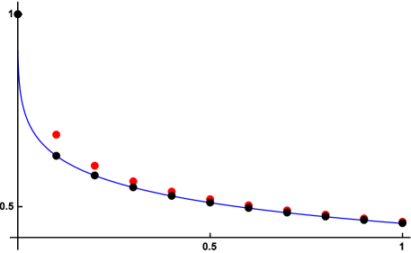
Figure 2: Graph of the analytical solution of equation (15) on the interval $[0,1]$ and numerical solutions (10)-red and the improved numerical solution (14)-black for (10), when $h=0.1$.

Table 5: Maximum error and order of numerical solutions (10) and (11) for equation (15) (left) and equation (17) (right).

$h$	$Error$	$Order$
$0.05$	$0.0496688$	$0.147528$
$0.025$	$0.0441259$	$0.170715$
$0.0125$	$0.0386498$	$0.191164$
$0.00625$	$0.0334386$	$0.208945$
$0.003125$	$0.0286254$	$0.224219$

$h$	$Error$	$Order$
$0.05$	$0.0840166$	$0.4486824$
$0.025$	$0.0567272$	$0.566632$
$0.0125$	$0.0365217$	$0.635288$
$0.00625$	$0.0229408$	$0.670839$
$0.003125$	$0.0142437$	$0.687593$

$\bullet$ Let $\alpha=0.7,m=3$ and $B=4.$

$$y^{(0.7)}(x)+4y(x)=0,\quad y(0)=1.$$ (17)

The maximum error and order of numerical solutions (10) and (11) for equation (17) are given in Table 5 (right). Substitute

$$z(x)=y(x)-1+\dfrac{4x^{0.7}}{\Gamma(1.7)}-\dfrac{16x^{1.4}}{\Gamma(2.4)}+\dfrac{64x^{2.1}}{\Gamma(3.1)}.$$

The function $z(x)$ is a solution of the equation

$$z^{(0.7)}(x)+z(x)=\dfrac{256x^{2.1}}{\Gamma(3.1)},\quad z(0)=0.$$ (18)

The maximum error and order of numerical solutions (10) and (11) for equation (18) are given in Table 7.

Table 6: Maximum error and order of numerical solutions (10) and (11) for equation (15).

$h$	$Error$	$Order$
$0.05$	$0.00022816$	$1.61147$
$0.025$	$0.00007356$	$1.63301$
$0.0125$	$0.00002347$	$1.64829$
$0.00625$	$7.43\times 10^{-6}$	$1.65956$
$0.003125$	$2.34\times 10^{-6}$	$1.66807$

$h$	$Error$	$Order$
$0.05$	$0.0000506703$	$1.88353$
$0.025$	$0.0000132354$	$1.93674$
$0.0125$	$3.39\times 10^{-6}$	$1.96378$
$0.00625$	$8.61\times 10^{-7}$	$1.97867$
$0.003125$	$2.17\times 10^{-7}$	$1.98724$

Table 7: Maximum error and order of numerical solutions (10) and (11) for equation (17).

$h$	$Error$	$Order$
$0.05$	$0.0825401$	$1.27437$
$0.025$	$0.0338612$	$1.28546$
$0.0125$	$0.0138328$	$1.29154$
$0.00625$	$0.0056374$	$1.29499$
$0.003125$	$0.0022943$	$1.29701$

$h$	$Error$	$Order$
$0.05$	$0.00682601$	$2.21359$
$0.025$	$0.00136314$	$2.32411$
$0.0125$	$0.00024704$	$2.46412$
$0.00625$	$0.00004329$	$2.51272$
$0.003125$	$7.24\times 10^{-6}$	$2.57940$

4 Numerical Solutions of the Fractional Subdiffusion Equation

The time-fractional subdiffusion equation is a parabolic partial fractional differential equation obtained from the heat equation by replacing the time derivative with a fractional derivative of order $\alpha$, where $0<\alpha<1$,

$$\dfrac{\partial^{\alpha}u(x,t)}{\partial t^{\alpha}}=\dfrac{\partial^{2}u(x,t)}{\partial x^{2}}.$$ (19)

The analytical solution of the fractional subdiffusion equation with initial and boundary conditions

$$u(x,0)=u_{\_}0(x),\;u(0,t)=u(\pi,t)=0,$$

is determined using the separation of variables method

$$u(x,t)=\sum_{\_}{n=1}^{\infty}c_{\_}nE_{\_}\alpha(-n^{2}t^{\alpha})\sin(nx),$$

where

$$c_{\_}n=\dfrac{2}{\pi}\int_{\_}0^{1}u_{\_}0(\xi)\sin(n\xi)d\xi.$$

Each term $E_{\_}\alpha(-n^{2}t^{\alpha})\sin nx$ is a solution of (19) and the coefficient $c_{\_}n$ is the coefficient of the Fourier sine series of the function $u_{\_}0(x)$. When $u_{\_}0(x)=\sin x$, the subdiffusion equation (2) has analytical solution $u(x,t)=\sin xE_{\_}\alpha(-t^{\alpha})$. In section 3 we used the fractional Taylor polynomials of the solution of the relaxation equation to improve the accuracy of numerical solutions (10) and (11). In this section we use the fractional Taylor polynomials of the solution of the subdiffusion equation in the time direction for improving the accuracy of difference approximations (20) and (21).

Let $h=\pi/N,\tau=1/M$, where $M$ and $N$ are positive integers, and $\mathcal{G}$ be a grid on the rectangle $[0,\pi]\times[0,1]$

$$\mathcal{G}=\left\{(nh,m\tau)\|1\leq n\leq N,1\leq m\leq M\right\}.$$

In [13] we determined the finite difference approximations (20) and (21) for the the fractional subdiffusion equation

$$\left\{\begin{array}[]{l l}\dfrac{\partial^{\alpha}u(x,t)}{\partial t^{\alpha}}=\dfrac{\partial^{2}u(x,t)}{\partial x^{2}}+F(x,t),&\\ u(x,0)=u_{\_}0(x),\;u(0,t)=u(\pi,t)=0.&\\ \end{array}\right.$$

Denote by $u_{\_}n^{m}$ and $F_{\_}n^{m}$ the values of the functions $u(x,t)$ and $F(x,t)$ on $\mathcal{G}$.

$$u_{\_}n^{m}=u(nh,m\tau),\quad F_{\_}n^{m}=F(nh,m\tau).$$

Let

$$\eta=\Gamma(2-\alpha)\dfrac{\tau^{\alpha}}{h^{2}},$$

$K$ be the tridiagonal matrix of dimension $N-1$ with values $1+2\eta$ on the main diagonal, and $-\eta$ on the diagonals above and below the main diagonal

$$K_{\_}{5}=\begin{pmatrix}1+2\eta&-\eta&0&0&0\\ -\eta&1+2\eta&-\eta&0&0\\ 0&-\eta&1+2\eta&-\eta&0\\ 0&0&-\eta&1+2\eta&-\eta\\ 0&0&0&-\eta&1+2\eta\end{pmatrix}$$

and $V^{0}$ be the vector of dimension $N-1$ determined from the initial condition

$$V^{0}=\left[u_{\_}0(nh)\right]_{\_}{n=1}^{N-1}.$$

The difference approximation for the subdiffusion equation $\left\{V^{m}\right\}$ using the $L1$ approximation (3) is computed with the linear system

$$KV^{m}=R_{\_}1,$$ (20)

where $R_{\_}1$ is the vector

$$R_{\_}1=\left[-\sum_{\_}{k=1}^{m}\sigma_{\_}k^{(\alpha)}V_{\_}n^{m-k}+\tau^{\alpha}\Gamma(2-\alpha)F_{\_}n^{m}\right]_{\_}{n=1}^{N-1}.$$

The numerical solution $\left\{W^{m}\right\}$ of the subdiffusion equation using the modified $L1$ approximation (4) is computed with the linear system

$$(K-\zeta(\alpha-1)I)W^{m}=R_{\_}2,$$ (21)

for $2\leq m\leq N-1$, where $R_{\_}2$ is the vector

$$R_{\_}2=\left[-\sum_{\_}{k=1}^{m}\delta_{\_}k^{(\alpha)}W_{\_}n^{m-k}+\tau^{\alpha}\Gamma(2-\alpha)F_{\_}n^{m}\right]_{\_}{n=1}^{N-1},$$

and $W^{0}=V^{0},W^{1}=V^{1}$.

When the solution of the subdiffusion equation is a sufficiently differentiable function, the difference approximations (20) and (21) have accuracy $O\left(\tau^{2-\alpha}+h^{2}\right)$ and $O\left(\tau^{2}+h^{2}\right)$. The solution of subdiffusion equation $\eqref{S1}$ has an unbounded first derivative at $t=0$. The numerical experiments in section 2 with $\alpha=0.5$ and other values of $\alpha\in(0,1)$ indicate that the accuracy of numerical solutions (20) and (21) is $O\left(\tau+h^{2}\right)$.

Let $D_{\_}t^{\beta}u(x,t)$ be the Miller-Ross derivative of order $\beta$ of the function $u(x,t)$ in the time direction.

$$D_{\_}t^{\alpha}u(x,t)=\dfrac{\partial^{2}u(x,t)}{\partial x^{2}}.$$

Then

$$D_{\_}t^{2\alpha}u(x,t)=D_{\_}t^{\alpha}D_{\_}t^{\alpha}u(x,t)=D_{\_}t^{\alpha}\dfrac{\partial^{2}u(x,t)}{\partial x^{2}}=\dfrac{\partial^{2}}{\partial x^{2}}D_{\_}t^{\alpha}u(x,t)=\dfrac{\partial^{4}u(x,t)}{\partial x^{4}},$$

$$D_{\_}t^{3\alpha}u(x,t)=D_{\_}t^{\alpha}D_{\_}t^{2\alpha}u(x,t)=D_{\_}t^{\alpha}\dfrac{\partial^{4}u(x,t)}{\partial x^{4}}=\dfrac{\partial^{4}}{\partial x^{4}}D_{\_}t^{\alpha}u(x,t)=\dfrac{\partial^{6}u(x,t)}{\partial x^{6}}.$$

In this way we obtain

$$D_{\_}t^{n\alpha}u(x,t)=\dfrac{\partial^{2n}u(x,t)}{\partial x^{2n}}.$$

Set $t=0$

$$D_{\_}t^{n\alpha}u(x,0)=\dfrac{\partial^{2n}u(x,0)}{\partial x^{2n}}=\dfrac{\partial^{2n}\sin x}{\partial x^{2n}}=(-1)^{n}\sin x.$$

From the fractional Taylor polynomials approximation

$$u(x,h)\approx\sin x\sum_{\_}{n=0}^{m}(-1)^{n}\dfrac{h^{n\alpha}}{\Gamma(n\alpha+1)},$$

when $h>0$ is a sufficiently small number. Substitute

$$v(x,t)=u(x,t)-\sin x\sum_{\_}{n=0}^{m}(-1)^{n}\dfrac{t^{n\alpha}}{\Gamma(n\alpha+1)}.$$

We have that

$$D_{\_}t^{\alpha}v(x,t)=D_{\_}t^{\alpha}u(x,t)+\sin x\sum_{\_}{n=0}^{m-1}(-1)^{n+1}\dfrac{t^{n\alpha}}{\Gamma(n\alpha+1)},$$

$$\dfrac{\partial^{2}}{\partial x^{2}}v(x,t)=\dfrac{\partial^{2}}{\partial x^{2}}u(x,t)+\sin x\sum_{\_}{n=0}^{m}(-1)^{n+1}\dfrac{t^{n\alpha}}{\Gamma(n\alpha+1)}.$$

The function $v(x,t)$ is a solution of the fractional subdiffusion equation

$$\left\{\begin{array}[]{l l}\dfrac{\partial^{\alpha}v(x,t)}{\partial t^{\alpha}}=\dfrac{\partial^{2}v(x,t)}{\partial x^{2}}+(-1)^{m+1}\sin x\dfrac{t^{m\alpha}}{\Gamma(m\alpha+1)},&\\ v(x,0)=v(0,t)=v(\pi,t)=0.&\\ \end{array}\right.$$

When $\alpha=0.3$ and $m=7$, the fractional subdiffusion equation

$$\left\{\begin{array}[]{l l}\dfrac{\partial^{0.3}u(x,t)}{\partial t^{0.3}}=\dfrac{\partial^{2}u(x,t)}{\partial x^{2}},&\\ u(x,0)=\sin x,\;u(0,t)=u(\pi,t)=0,&\\ \end{array}\right.$$ (22)

has analytical solution $u(x,t)=\sin xE_{\_}{0.3}\left(-t^{0.3}\right)$. The difference approximations (20) and (21) for equation (22) have accuracy $O(\tau)$ in the time direction (Table 8 (left) and Table 9 (left)). Let

$$v(x,t)=u(x,t)-\sin x\sum_{\_}{n=0}^{7}(-1)^{n}\dfrac{h^{0.3n}}{\Gamma(0.3n+1)}.$$

The function $v(x,t)$ is a twice continuously differentiable function and is a solution of the homogeneous subdiffusion equation

$$\left\{\begin{array}[]{l l}\dfrac{\partial^{0.3}v(x,t)}{\partial t^{0.3}}=\dfrac{\partial^{2}v(x,t)}{\partial x^{2}}+\sin x\dfrac{t^{2.1}}{\Gamma(3.1)},&\\ v(x,0)=v(0,t)=v(\pi,t)=0.&\\ \end{array}\right.$$ (23)

In Table 8 (right) and Table 9 (right) we compute the maximum error and numerical order of difference approximations (20) and (21) for the fractional subdiffusion equation (23) on the rectangle

$$(x,t)\in[0,\pi]\times[0,1],$$

with step size in the space direction $h=\pi\tau/3$. Numerical experiments with other values of the step sizes $h$ and $\tau$ confirm that the numerical solutions (20) and (21) converge to the analytical solution of the fractional subdiffusion equation (23) with the expected accuracy $O\left(\tau^{2-\alpha}+h^{2}\right)$ and $O\left(\tau^{2}+h^{2}\right)$. A question for future work is to extend the method presented in this paper to other ordinary and partial fractional differential equations.

Table 8: Maximum error and order of numerical solution (20) of equations (22) (left) and (23) (right), for $h=\pi\tau/3$, at time $t=1$.

$\tau$	$Error$	$Order$
$0.05$	$0.00208324$	$1.08653$
$0.025$	$0.00100782$	$1.04759$
$0.0125$	$0.00049480$	$1.02633$
$0.00625$	$0.00024489$	$1.01468$
$0.003125$	$0.00012175$	$1.00826$

$\tau$	$Error$	$Order$
$0.05$	$0.000247016$	$1.64590$
$0.025$	$0.000078268$	$1.65812$
$0.0125$	$0.000024643$	$1.66722$
$0.00625$	$7.72\times 10^{-6}$	$1.67411$
$0.003125$	$2.41\times 10^{-6}$	$1.67940$

Table 9: Maximum error and order of numerical solution (21) of equations (22) (left) and (23) (right), for $h=\pi\tau/3$, at time $t=1$.

$\tau$	$Error$	$Order$
$0.05$	$0.001565250$	$1.05230$
$0.025$	$0.000760933$	$1.04055$
$0.0125$	$0.000372634$	$1.03001$
$0.00625$	$0.000183395$	$1.02281$
$0.003125$	$0.000090563$	$1.01796$

$\tau$	$Error$	$Order$
$0.05$	$0.000031877$	$1.81175$
$0.025$	$8.54\times 10^{-6}$	$1.90107$
$0.0125$	$2.22\times 10^{-6}$	$1.94430$
$0.00625$	$5.67\times 10^{-7}$	$1.96751$
$0.003125$	$1.44\times 10^{-7}$	$1.98068$

References

• [1] A. Cartea, D. del Castillo-Negrete, Fractional diffusion models of option prices in markets with jumps. Physica A, 374(2) (2007), 749–763.
• [2] O. Marom, E. Momoniat, A comparison of numerical solutions of fractional diffusion models in finance, Nonlinear Analysis: Real World Applications, 140(6) (2009), 3435–3442.
• [3] F, Mainardi, Fractional relaxation-oscillation and fractional diffusion-wave phenomena, Chaos, Solitons $\&$ Fractals, 7(9) (1996), 1461 – 1477.
• [4] S. I. Muslih, Om P. Agrawal, D. Baleanu, A fractional SchrΓΆdinger equation and its solution, International Journal of Theoretical Physics, 49(8) (2010), 1746–1752.
• [5] P. M. Lima, N. J. Ford, and P. M. Lumb, Computational methods for a mathematical model of propagation of nerve impulses in myelinated axons, Applied Numerical Mathematics 85, (2014), 38–53.
• [6] W. Deng, C. Li, Numerical Schemes for Fractional Ordinary Differential Equations, In Numerical Modeling, Peep Miidla (editor). InTech; 2012.
• [7] K. Diethelm, The Analysis of Fractional Differential Equations: An Application-Oriented Exposition Using Differential Operators of Caputo Type. Springer; 2010.
• [8] K.S. Miller, B. Ross, An Introduction to the Fractional Calculus and Fractional Differential Equations. John Wiley & Sons, New York; 1993.
• [9] I. Podlubny, Fractional Differential Equations. Academic Press, San Diego; 1999.
• [10] A. El-Ajou, O. Arqub, Z. Zhour and S. Momani, New results on fractional power series: theory and applications, Entropy, 15, (2013), 5305-5323.
• [11] J. Cao, C. Xu, A high order schema for the numerical solution of the fractional ordinary differential equations, Journal of Computational Physics, 238(1), (2013), 154–168.
• [12] Y. Dimitrov, Numerical approximations for fractional differential equations, Journal of Fractional Calculus and Applications, 5(3S), (2014), No. 22, 1–45.
• [13] Y. Dimitrov, A second order approximation for the Caputo fractional derivative, arXiv:1502.00719, (2015).
• [14] M. GΓΌlsu, Y. Γ–ztΓΌrk, A. AnapalΔ±, Numerical approach for solving fractional relaxation–oscillation equation, Applied Mathematical Modelling 37, (2013) 5927–5937.
• [15] H. Hejazi, T. Moroney, F. Liu, Stability and convergence of a finite volume method for the space fractional advection–dispersion equation, Journal of Computational and Applied Mathematics, 255, (2014), 684 – 697.
• [16] B.Jin, R. Lazarov and Z. Zhou, An analysis of the $L1$ scheme for the subdiffusion equation with nonsmooth data, arXiv:1501.00253, (2015).
• [17] C. Li, A. Chen, J. Ye, Numerical approaches to fractional calculus and fractional ordinary differential equation, Journal of Computational Physics, 230(9), (2011), 3352 – 3368.
• [18] Y. Lin and C. Xu. Finite difference/spectral approximations for the time-fractional diffusion equation. Journal of Computational Physics, 225(2), (2007), 1533–1552.
• [19] R. Lin, F. Liu, Fractional high order methods for the nonlinear fractional ordinary differential equation, Nonlinear Analysis: Theory, Methods & Applications, 66(4), (2007), 856–869.
• [20] N. F. Martins, M. L. Morgado and M. Rebelo, A meshfree numerical method for the time-fractional diffusion equation, Proceedings of the 13th International Conference on Computational and Mathematical Methods in Science and Engineering, CMMSE 2013, 24–27 June, 2013.
• [21] S.B. Yuste, J. Quintana-Murillo, A finite difference method with non-uniform timesteps for fractional diffusion equations, Computer Physics Communications, 182, 2594 (2012)
• [22] J. Quintana-Murillo, S.B. Yuste, A finite difference method with non-uniform timesteps for fractional diffusion and diffusion-wave equations, Eur. Phys. J. Special Topics 222, (2013), 1987–1998.
• [23] B.Jin, R. Lazarov and Z. Zhou, Two fully discrete schemes for fractional diffusion and diffusion-wave equations, arXiv:1404.3800, (2015).
• [24] Z. Odibat, N. Shawagfeh, Generalized Taylor’s formula, Applied Mathematics and Computation 186, (2007), 286–293.
• [25] T. J. Osler, Taylor’s series generalized for fractional derivatives and applications, SIAM J. Math. Anal., 2(1), (1971), 37–-48.
• [26] J. E. PečariΔ‡, I. PeriΔ‡, H.M. Srivastava, A family of the Cauchy type mean-value theorems, Journal of Mathematical Analysis and Applications, 306(2), (2005), 730–739.
• [27] M. Stynes, J. L. Gracia, Boundary layers in a two-point boundary value problem with a Caputo fractional derivative, Comput. Methods Appl. Math., 15 (1), (2015), 79–95.
• [28] Z.-Z. Sun, X. Wu, A fully discrete scheme for a diffusion wave system, Applied Numerical Mathematics, 56(2), (2006), 193–209.
• [29] J. Rena, Z.-Z. Sun, Maximum norm error analysis of difference schemes for fractional diffusion equations, Applied Mathematics and Computation, 256, (2015) 299–314.
• [30] J.J. Trujillo, M. Rivero, B. Bonilla, On a Riemann–Liouville generalized Taylor’s formula, Journal of Mathematical Analysis and Applications, 231(1), (1999), 255–265.
• [31] P. Zhuang, F. Liu, Implicit difference approximation for the time fractional diffusion equation, Journal of Applied Mathematics and Computing, 22(3), (2006), 87–99.