GRO J1744-28: an intermediate B-field pulsar in a low mass X-ray binary

Abstract

The bursting pulsar, GRO J1744-28, went again in outburst after $\sim$18 years of quiescence in mid-January 2014. We studied the broad-band, persistent, X-ray spectrum using X-ray data from a XMM-Newton observation, performed almost at the peak of the outburst, and from a close INTEGRAL observation, performed 3 days later, thus covering the 1.3–70.0 keV band. The spectrum shows a complex continuum shape that cannot be modelled with standard high-mass X-ray pulsar models, nor by two-components models. We observe broadband and peaked residuals from 4 to 15 keV, and we propose a self-consistent interpretation of these residuals, assuming they are produced by cyclotron absorption features and by a moderately smeared, highly ionized, reflection component. We identify the cyclotron fundamental at $\sim$ 4.7 keV, with hints for two possible harmonics at $\sim$ 10.4 keV and $\sim$ 15.8 keV. The position of the cyclotron fundamental allows an estimate for the pulsar magnetic field of (5.27 $\pm$ 0.06) $\times$ 10¹¹ G, if the feature is produced at its surface. From the dynamical and relativistic smearing of the disk reflected component, we obtain a lower limit estimate for the truncated accretion disk inner radius, ($\gtrsim$ 100 R_g), and for the inclination angle (18^∘–48^∘). We also detect the presence of a softer thermal component, that we associate with the emission from an accretion disk truncated at a distance from the pulsar of 50–115 R_g. From these estimates, we derive the magneto-spheric radius for disk accretion to be $\sim$ 0.2 times the classical Alfvén radius for radial accretion.

1 Introduction

Mildly-recycled, slowly spinning, accreting X-ray pulsars in low-mass X-ray binaries (LMXBs) are uncommon objects, because of the relatively short time required to spin up the neutron star (NS) to frequencies $f_{spin}$ $>$ 100 Hz during the X-ray active phase. Before, or simultaneously, with this recycling phase, the magnetic field (B-field) of the NS decays from values B $\gtrsim$ 10¹² G, typical of young NS in high-mass X-ray binaries (HMXBs), down to B $\lesssim$ 10⁸ G, when the strength of the field is no longer able to significantly drive the accretion flow and coherent pulsations in the persistent emission are no longer detected.

Our current understanding of how NS B-fields are actually dissipated is not yet complete (Payne & Melatos 2004; Zhang & Kojima 2006), so that the study of LMXBs where measures of the B-field are possible are of extreme importance. Direct and indirect methods for the determination of the B-field are possible if pulsations are detected, as in the case of recycled LMXBs that host fast spinning NSs (the class of the accreting millisecond X-ray pulsars, AMXPs) and for a smaller group of LMXBs where the process of recycling is probably caught in its very early stage, and the NS spin frequency is much below 100 Hz (Patruno et al. 2012). Members of this class are e.g. the 1.7 Hz pulsar in X1822-371, where the mass transfer is probably highly non-conservative and at super-Eddington rates (Burderi et al. 2010; Iaria et al. 2013); the 11 Hz pulsar in IGR J1748-2446 (Papitto et al. 2011); the 0.13 Hz pulsar in 4U 1626-67 (Beri et al. 2014); the 0.8 Hz pulsar in the well-known system Her X-1 (Tananbaum et al. 1972) and the 2.14 Hz pulsar in GRO J1744-28 (Degenaar et al. 2014).

GRO J1744-28 was discovered in hard X-rays (25–60 keV) by BATSE/CGRO on 2nd, December 1995 (Kouveliotou et al. 1996) as a bursting source. Bursts were soon associated to unstable/spasmodic accretion episodes (type-II bursts, Kouveliotou et al. 1996; Lewin et al. 1996). Finger et al. (1996) discovered coherent pulsations at 2.14 Hz and its Doppler modulation, leading to the determination of the orbital period (11.8337 days), eccentricity ($e$ $<$ 1.1 $\times$ 10^-3), projected semi-major axis (2.6324 lt-s), and mass function (1.3638 $\times$ 10^-4 M_⊙). The pulsed profile showed a nearly sinusoidal shape, which together with the value of the mass function, implies the inclination angle, or the companion mass, or both these conditions, to have low values.

We observed to date three major X-ray outbursts from GRO J1744-28: the first associated with its discovery lasting from December 1995 to May 1996, where at the peak outburst reached over-Eddington luminosities (Jahoda et al. 1999; Giles et al. 1996; Woods et al. 1999; Woods et al. 2000); the second outburst occurred about one year later, started at the beginning of December 1996 and lasted about four months. A long period of quiescence followed, interrupted by the third and most recent outburst observed in January 2014.

It was soon realized, just after its discovery, that the low spin period, the long orbital period and the observed flux and spin derivative are all factors that point to an intermediate B-field pulsar (10¹¹ G $<$ B $<$ 10¹² G) in a low inclination system (Daumerie et al. 1996). Cui (1997) presented observational evidence for a propeller effect during the decay period of the first outburst, where pulsations were not detected below a flux of 2.3 $\times$ 10^-9 erg cm^-2 s^-1 (2-60 keV), from which a rough limit on the Alfvén radius could be derived, and thus leading to a B-field estimate of $\sim$ 2.4 $\times$ 10¹¹ G, assuming a distance of 8 kpc. Rappaport & Joss (1997) presented possible evolutionary paths for GRO J1744-28 that could lead to the formation of the presently observed system, and starting from a set of reasonable initial conditions, gave rather tight limits on the possible companion mass (0.2–0.7 M_⊙), neutron star mass (1.4–2.0 M_⊙), inclination angle (7^∘–22^∘) and pulsar B-field (1.8–7 $\times$ 10¹¹ G).

Search for the optical/NIR counterpart has been difficult because of the crowded Galactic Centre field where GRO J1744-28 resides. $Chandra$ and XMM-Newton detected a low-level (1–3 $\times$ 10³³ erg s^-1) persistent X-ray activity in 2002 (Wijnands & Wang 2002; Daigne et al. 2002), allowing to refine the estimates on the source coordinates. Degenaar et al. (2012) reported enhanced flux (L_X $\sim$ 1.9 $\times$ 10³⁴ erg s^-1) in September 2008. Gosling et al. (2007) determined two near-infrared possible candidate sources within the $Chandra$ error circle. Most recent determinations (Masetti et al. 2014) indicate that the candidate source $a$ by Gosling et al. (2007) is the likely counterpart. Hence, the companion star is an evolved G/K III star. GRO J1744-28 has been associated to the Galactic Centre population, setting its distance at $\sim$ 7.5 kpc (Augusteijn et al. 1997).

One of the main peculiarity of GRO J1744-28 is the presence of Type-II bursts (Lewin et al. 1996). Cannizzo (1997) identified the Lightman-Eardley instability occurring at the magnetospheric radius in the accretion disk as the possible cause of the bursting behaviour. Bildsten & Brown (1997) argued for the possible presence of type-I bursts together with the type-II as observed also for the Rapid Burster for accretion rates lower than 6 $\times$ 10^-9 M_⊙ yr^-1. The bursts have similar structures, with a fast rising (few seconds), a peak emission that lasts few seconds and a tail that appears as a dip with respect to the pre-burst average count rate. During the bursts the pulsed fraction increases but the phase with the pre-outburst pulsations is not maintained, leading to the unusual phenomenon of pulsar glitches (Stark et al. 1996).

The X-ray continuum emission of GRO J1744-28 during the 1996 outburst has been studied using the low energy-resolution $RXTE$/PCA data. Giles et al. (1996) modelled this spectrum using an absorbed power-law with a high-energy cut-off (E_cut = 20 keV, E_fold = 15 keV). They also found a pulse-dependent photon-index between 1.20 $\pm$ 0.02 (at the peak of the pulsed emission) and 1.35 $\pm$ 0.01 (at the pulse minimum), and detected a broad ($\sigma\sim$ 1 keV) Gaussian emission line in the Fe K$\alpha$ region. Nishiuchi et al. (1999) presented a spectroscopic investigation with ASCA data for two different dates and accretion rates. They found the line to be intrinsically broad and they proposed a relativistically smeared reflection component as the cause of the broadening. The iron line profile was compatible with resonant emission from mildly ionized iron for the first observation, whereas highly ionized (6.7–6.97 keV) iron seemed preferred for the second observation. However, the best-fitting value for the inclination angle, $>$ 50^∘, seems unlikely because of the constraints on the mass function and companion’s spectral type. Similarly, the value for the inner disk radius, 10 R_g $<$ R_in $<$ 30 R_g) appears also unlikely because of the different indications for an intermediate NS B-field (Daumerie et al. 1996; Cui 1997; Rappaport & Joss 1997), that would truncate the disk at larger distances, so that other broadening mechanisms, or a more complex profile, have been additionally advocated.

Degenaar et al. (2014) reported from a recent high-resolution $Chandra$/HETGS observation the detection of an asymmetric line profile from He-like iron, and interpreted it as a disk reflected feature, from which an inner disk radius of 85 $\pm$ 11 R_g and an inclination angle of 52${}^{\circ}\,\pm\,4^{\circ}$ have been estimated. Younes et al. (2015) analysed the broadband spectrum of GRO J1744-28 with $NuSTAR$ and $Chandra$, fitting the continuum emission with a cut-off power-law of photon-index $\Gamma\sim$ 0, cut-off energy $\sim$ 7 keV, and a soft continuum thermal component at a temperature of 0.55 keV, interpreted as emission from the accretion disk. They also reported the presence of a significantly broadened ($\sigma$ = 3.7 keV) feature at $\sim$ 10 keV. Moderately broadened highly-ionized emission lines at 6.6 keV and 7.01 keV were also detected, together with emission from neutral iron at 6.4 keV.

The 2014 outburst of GRO J1744-28

Enhanced X-ray emission from the direction of the transient outbursting source GRO J1744-28 was detected from 18th, January 2014 with MAXI (Negoro et al. 2014). Pulsations at 2.14 Hz were detected in hard X-rays with FERMI/GBM monitor on 24th, January 2014 (Finger et al. 2014) and in soft X-rays with the $Swift$/XRT on 6th, February 2014 (D’Aì et al. 2014), confirming the association of the ongoing outburst with the bursting pulsar. The outburst reached its peak in mid-March, when the source was accreting close to the Eddington limit (Negoro et al. 2014) and from then it started to decline linearly until 23th April when the light curve as seen in the $Swift$/BAT monitor (Fig. 1) clearly showed a drop, and the profile became exponential with a decay time of $\sim$ 11 days. The outburst was regularly monitored by $Swift$ and $INTEGRAL$ satellites (Masetti et al. 2014). A Target of Opportunity observation with XMM-Newton observed the source from 6th 14:03:12.27 to 7th 13:29:50 March 2014, for a total exposure time of 83915 s. The observation was performed few days before the GRO J1744-28 flux reached the outburst peak as shown by the black thick arrow superimposed to the BAT light curve from MJD 56679 (22nd, January 2014) to MJD 56809 (1st, June 2014) in Fig. 1. For this work we also exploited data from an INTEGRAL observation (dotted arrow in Fig. 1) performed three days later the XMM-Newton pointing.

Figure 1: $Swift$-BAT (Krimm et al. 2013) daily light curve in the 15–50 keV range from 22nd January to 1st June 2014. The black thick (dotted) arrow marks the time of the XMM-Newton (INTEGRAL) observation.

2 Observation and data reduction

We used the Science Analysis System (SAS) version 13.5.0 and the calibration files (CCF) updated at March 2014 for the data extraction and analysis of the XMM-Newton data; we used the software package HeaSOFT version 6.15.1 for the timing analysis and for general purposes data reduction, and Xspec v.12.8.1 for spectral fitting.

The EPIC/pn operated in Timing Mode with the optical thick filter, while the Reflection Grating Spectrometer instruments (RGS1 and RGS2) in Spectroscopy Mode. The EPIC/MOS instruments were switched off to allow the highest possible telemetry for the EPIC/pn.

The RGS data were extracted using the rgsproc pipeline task. The total exposure for the RGS1 (RGS2) instrument is 83715 s (83750), and the first-order net light curves has an average count rate per second (cps) of 0.283 $\pm$ 0.002 (0.268 $\pm$ 0.002). Second-order count rates, for RGS1 and RGS2, are $\sim$ 30 % and $\sim$ 70 % the first-order rates, respectively. The bursts are not clearly resolved in the RGS light curves, because the source is strongly absorbed at lower energies and the RGS1 and RGS2 frame times are 4.59 s and 9.05 s, respectively, that are long compared to the rapid burst evolution.

The EPIC/pn event file was processed using the epproc pipeline processing task with the runepreject=yes, withxrlcorrection=yes, runepfast=no. and withrdpha=yes, as suggested by the most recent calibration status report (see also Pintore et al. 2014). The average count rate, corrected for telemetry gaps (epiclccorr tool), during the entire observation over all the EPIC/pn CCD was 714 cps. The EPIC/pn light curve shows 43 bursts during the entire observation with a mean rate of 0.53 burst hr^-1. Fig. 2 shows the first 20 ks of the EPIC/pn observation, where nine bursts are present. The bursts profiles can be clearly resolved, they have similar structures with an average rising time and typical peak duration of a few seconds. During these peaks the observed rate becomes so high that telemetry saturation and strong pile-up prevent a reliable analysis of the data.

The burst decay is well described by an exponential tail with decay-times in the range 2–10 s. The count rate after each burst drops about 10% with respect to the pre-burst level and returns to it slowly after few hundred seconds. Such behaviour and the burst characteristics are very close to the typical phenomenology shown by the source in the two past outbursts (Giles et al. 1996).

In Fig. 3 we show a snapshot of the EPIC/pn light curve encompassing two typical bursts (upper panel), and the hardness ratio (HR) evolution, where the soft color is defined in the energy range 0.5–4 keV and the hard color in the 4–10 keV range (lower panel). The light curve is corrected for telemetry saturation (epicclcorr task), and it is filtered removing the three hottest RAWX columns to limit pile-up effects at the burst peak.

Figure 2: EPIC/pn light curve for the first 20 ks of the observation. Bin time is 5 s.

Figure 3: Two consecutive bursts and relative hardness ratio (HR, 4.0–10.0/0.5–4.0 keV). Selected extraction region excludes the RAWX = [36:38] columns to avoid photon pile-up. Bin time is 5 s.

We focused on the persistent emission of the pulsar by time-filtering the EPIC/pn event list excluding appropriate intervals around the bursts. The excluded windows are all of 400 s length, starting a few seconds before the rising trail of the bursts. The final exposure, corrected also for telemetry drops, of the persistent emission resulted of 64130 s.

2.1 Timing analysis

We barycentred the EPIC/pn, burst-filtered, event file with respect to the Barycentric Dynamical Time (TDB) using the barycen tool with R.A. and DEC coordinates 266.137792 and -28.740803, respectively (Gosling et al. 2007). We used all the events that passed the filtering condition FLAG==0. A power spectrum of the persistent emission clearly reveals the pulsation at 2.14 Hz and the first harmonic at 4.28 Hz. To correct the pulse arrival times for the orbital motion of the pulsar, we used the following orbital parameters (GBM pulsar project): P_orb = 11.836397 d, a sin(i) = 2.637 lt-s, and T_π/2 = 56695.6988 MJD. We then used a folding search ($efsearch$ in XRONOS) to find the averaged pulse period during the persistent emission. The $\chi^{2}$ highest peak is found in correspondence with a period of 0.4670450(1) s, or 2.14112130(46) Hz, where the uncertainty corresponds to the step period search time (10^-7 s).

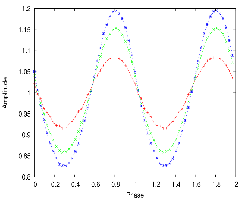
Figure 4: Top panel: energy-averaged pulse-folded profile (32 channels) and best-fitting model using two sinusoids. Bottom panel: pulse-folded profile for the EPIC/pn data in energy bands: 0.5–3.0 keV (red data), 3.0–6.0 keV (green data), and 6.0–12-0 keV (blue data).

To check possible shifts in the spin frequency during the observation, we folded at this period the persistent event file using a folding time window of 10⁴ pulse periods and the start time of the observation as epoch of reference. We then plotted the phases with respect to this folding period as a function of the time. The phases showed random scattering, and no other correction was found necessary. Folding the entire persistent emission at this period resulted in the folded profile of Fig. 4. The pulse shape can be well fitted as the sum of two sinusoids. Using the standard notation for the pulse amplitude $A$,

$$A=\frac{I_{max}-I_{min}}{I_{max}+I_{min}}$$ (1)

we found the fundamental has an amplitude of 15.1%, while the first harmonic amplitude is 0.91%, corresponding to $\sim$ 6% the fundamental. The folded profile is strongly energy dependent in the EPIC/pn band, as clearly shown in the bottom panel of Fig. 4, where the folded profile is obtained for three energy band: 0.5–3.0 keV, 3.0–6.0 keV and 6.0–12.0 keV.

2.2 The amplitude fraction

We studied the amplitude fraction as a function of energy for the EPIC/pn band. We exploited all the selected events in the RAWX columns, although we were aware that pile-up may distort the energy-dependent amplitude measures; however we estimated that the relative error induced by some fraction of pile-up events is significantly lower than the statistical uncertainties introduced when removing the hottest columns. We selected the pulse profiles in the pulse-invariant (PI) channel as follows: from 0.5 to 2 keV by a step of 0.5 keV, from 2 keV to 8 keV by a step of 0.25 keV, from 8 to 10.5 keV by a step of 0.5 keV, and from 10.5 keV to 12 keV into a single profile.

We folded the persistent event file using our best period estimate (0.4670450 s) and fitted the resulting pulse shape using two sinusoids. In Fig. 5 we show the dependence of the amplitude of the fundamental and first harmonic as a function of the energy.

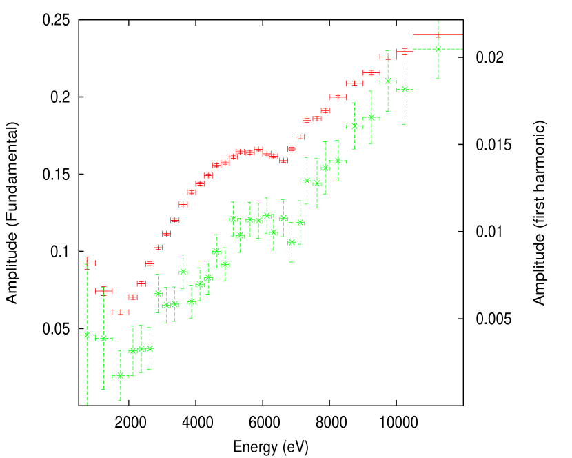
Figure 5: Amplitude fraction for the fundamental (red data, left y-axis) and first harmonic (green data, right y-axis) as a function of the energy.

It is evident that above 2 keV the pulse amplitude strongly correlates with energy, with the exception of the energy range between 6 and 7 keV where a remarkable drop in amplitude is present. To better characterize the shape of this drop we used a phenomenological model to describe the amplitude dependence in the 2.0–5.5 and 7.5–12 keV range. We described this trend using a polynomial fit, attaining a $\chi^{2}\sim$ 1 with a third order polynomial. We show in Fig. 6, the residuals of this fit when the data of the 5.5–7.5 keV region are then noticed. The shape of the residuals is consistent with a Gaussian profile, that it is centred at $\sim$ 6.5 keV and has a sigma of $\sim$ 0.8 keV. This drop indicates the presence of a spectral component that is not pulsed, and we shall show that its shape is compatible with the shape of a disk reflection component as derived from the analysis of the broadband spectrum (see Sect. 3.5).

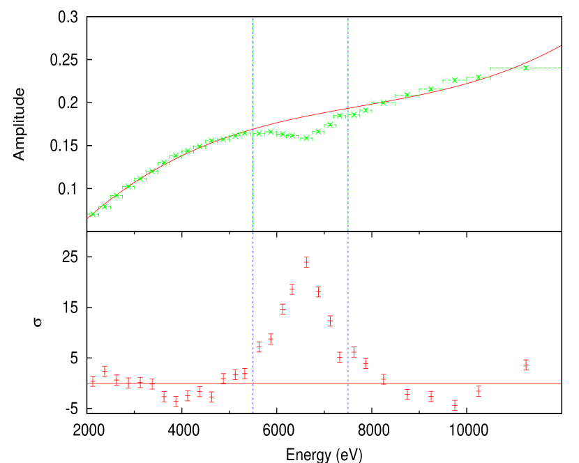
Figure 6: Upper panel: fundamental amplitude as a function of energy in the 2.0–12.0 keV range, super-imposed with the best-fitting trend derived by data in the same range, excluding the interval 5.5–7.5 keV. Lower panel: residuals in units of sigma for the 5.5–7.5 keV range for the best-fitting model consisting of a third degree polynomial derived by fitting the data in the 2.0–5.5 keV and 7.5–12 keV range.

3 Spectral analysis

3.1 RGS data analysis

RGS count rates are always below the threshold for photon pile-up. Because of the higher spectral resolution of the RGS detector with respect to the EPIC/pn and the low-energy coverage in a region where the effect of ISM absorption is the highest and the EPIC/pn spectrum is affected by larger systematics, we first performed a preliminary spectral analysis in this restricted energy band. We extracted first and second order RGS spectra of the persistent emission using the same good time intervals obtained from the EPIC/pn light curve. We looked at the background contribution to choose the noticed energy ranges for spectral fitting, keeping channels above $\sim$ 3 $\sigma$ the background value. Using a simple model consisting of an absorbed power-law and a constant of normalization free to vary for the different datasets, we found this inter-calibration factor among the four spectra variable at the 7% level.

We verified the consistency of the RGS1/RGS2 spectra and generated a combined spectrum using the SAS rgscombine tool for the first (RGSo1) and second (RGSo2) order spectra. After having verified that the persistent spectrum is, within the statistical uncertainties, consistent with the total time-averaged spectrum, to increase the statistical weight of the RGS data, we used this time averaged spectrum for the rest of our analysis. We found no evident emission/absorption narrow feature, so that we chose to group the spectra to a minimum of 100 counts/channel. Both spectra (first and second orders summed) are used in the 1.3–2.0 keV range, because below 1.3 keV the spectrum becomes background-dominated.

3.2 EPIC/pn data analysis: pile-up and background issues

Because of the high count rate recorded by the EPIC/pn instrument, we checked the pile-up level of the persistent time-averaged emission. In the EPIC/pn Timing mode spatial information is collapsed into one dimension (RAWX coordinate), while spectral extraction is usually performed in a 2-dimensional array, using the RAWY coordinate, that, however, is a temporal coordinate.

The point-spread function in the RAWX-RAWY image peaks for the RAWX=37 column and we created four filtered spectra selecting the RAWX=[28:46] region, and successively removing one, three, and five central columns, accompanied always by the filtering expressions PATTERN$\leq$4 and (FLAG==0). We obtained response matrices using the rmfgen tool and the ancillary files using the arfgen tool, following standard pipelines.

For each filtered event list, we applied the epatplot tool and we noted that the exclusion of three central columns provided a spectrum with an observed-to-model singles and doubles pattern fraction close to unity. However, we noted that the choice of excising the PSF caused severe effects on the continuum spectral determination. In fact, when the spectra were comparatively examined, it resulted evident that the removal of central columns softened the spectrum beyond what could be expected by the pile-up correction. We probed this by means of spectral analysis. In Fig.7, we show the spectra extracted from the EPIC/pn using all the RAWX[28:46] columns (full spectrum), and removing the three hottest columns, together with a $\sim$ 1 ks $Swift$/XRT spectrum (WT mode) taken on March 7th (OBS.ID 00030898022) in a simultaneous time window with XMM-Newton. We note here that the averaged count rate for the $Swift$/XRT spectrum was $\sim$ 70 cps, which is considerably below the threshold limit ($\sim$ 100 cps) for the WT mode photon pile-up, and the spectrum can be considered a bona fide benchmark.

The excised spectrum clearly displays a strong flux drop above 7 keV that is not observed in the $Swift$/XRT spectrum. The color ratio of the 2.0-6.0/6.0-10.0 keV absorbed flux is 0.61 for the spectrum without excision, and 0.69 for the spectrum with three columns removed, while for the $Swift$/XRT spectrum we measured a value of 0.63, that is much more consistent with the spectrum with no removed column. We argue that, although some level of pile-up could be present, the choice of excising the PSF artificially introduces spectral distortions, possibly related to the reconstruction of the energy-dependent ancillary response, that becomes more significant than the eventual pile-up correction. We choose therefore to use the whole PSF extraction region for spectral analysis, but we will also show the best-fitting results for the three-columns excised spectrum, to have a rough estimate of the sensitivity due to these instrumental issues on the determination of the physical parameters. Because the EPIC/pn full spectrum contains $\sim$ 5$\times$10⁷ counts, statistical errors become possibly dominated by systematic errors of the response matrix and, to account for this, and obtain final $\chi^{2}$ close to 1, we added a 0.5 % systematic error to the EPIC/pn channels (see also Hiemstra et al. 2011).

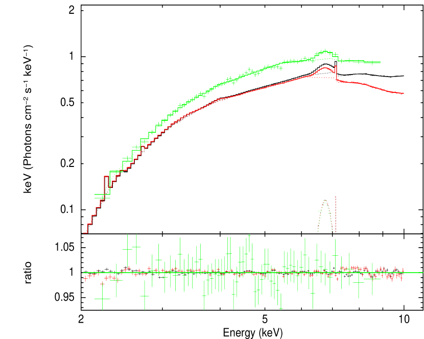
Figure 7: Data, unfolded spectra and data/model ratio for the EPIC/pn spectrum extracted from the whole PSF (no columns removed, black data), for the EPIC/pn spectrum extracted from the wings of the PSF (three columns removed, red data), and for the $Swift$/XRT spectrum from a simultaneous observation (green data).

It is suggested to extract the background spectrum from the first columns (e.g. selecting RAWX columns between 2 and 6) of the RAWX-RAWY image, however the flux of the source is severe, causing considerable spreading of the point spread function leading to contamination of source photons even in these first columns. Light curves extracted from this region and from central columns do in fact show a very significant positive correlation (p-value $<$ 2.2e-16). To obtain a measure of the expected level of background, we used a 2001 XMM-Newton observation covering the field of view of GRO J1744-28 (Obs.ID 0112971201) of $\sim$ 3 ks performed with the EPIC/pn in Imaging Mode (Full-Frame). In this observation the source is quiescent and no other point source is detected in a 5′region around the source coordinates. We extracted a spectrum around the coordinates of the source using a circular region of 2.4′radius, thus covering the same geometric area of our selection.

We fitted this spectrum using a phenomenological model of a broken power-law, obtaining a satisfactory description of the data with a reduced $\chi^{2}$ = 1.1 for 112 d.o.f. We used this best-fitting model to generate a faked background spectrum using the same response matrix, ancillary response, and time integration of the source spectrum. We thus verified that the expected background contribution compared with the observed source flux is very small in all the EPIC/pn range, contributing $\sim$ 1% below 2 keV and $\sim$ 0.2% above. The background spectrum extracted from the first columns contributes $\sim$ 2% above 2 keV, so although some variability in the region around the source can be expected, we argue that the background subtraction may affect the source flux determination with this level of uncertainty. We finally verified that setting no background for the EPIC/pn spectrum had no significant impact for the determination of the spectral parameters reported in the analysis.

Finally, we re-binned the spectrum in order to have at least 25 counts/channel and set the oversampling at 3 channels/energy resolution with the specgroup tool. We quoted spectral errors at $\Delta\chi^{2}$ = 2.7, if not stated otherwise.

3.3 Spectral Analysis of the Persistent Phase-Averaged Emission

We first studied the persistent, pulse-averaged, spectrum. For spectral analysis, we used the 1.3–2.0 keV range of the RGS spectra and the 2.0–9.5 keV range for the EPIC/pn spectrum. We first noted that the EPIC/pn data below 2 keV do not well match the RGS spectrum, and this mismatch can be modelled by an non-physical soft excess present in the EPIC/pn data that is not required in the RGS. Such mismatch has been reported in many other Timing Mode observations of highly absorbed (N_H $>$ 10²² cm^-2) sources (see e.g. D’Aì et al. 2010), and it has been investigated in one of the most recent calibration technical reports of the EPIC/pn team (CAL-TN-0083). Although we carefully applied the suggested corrections to the EPIC/pn processing pipeline, still the residuals do clearly point to the presence of this instrumental artefact, probably enhanced by the high statistics of the EPIC/pn spectrum. Because the spectrum below 2 keV is well covered by the RGS data (Fig. 9), that do not suffer from any known instrumental issue, we chose to discard EPIC/pn data below 2 keV. Because the source is highly absorbed, we found that the choice of the abundance table is quite relevant for determining the absolute value of the equivalent hydrogen column and the slope of the continuum emission as well, given the high correlation between these parameters. We used the tbabs model and tried all the different abundance tables available for Xspec, setting the cross-section table to that of Verner et al. (1996). We derived first some estimates using only the RGS datasets and a simple power-law continuum, obtaining values for equivalent column between (6.24 $\pm$ 0.07) $\times$ 10²² cm^-2, adopting the Anders & Grevesse (1989) table, to (9.68 $\pm$ 0.40) $\times$ 10²² cm^-2, adopting the Wilms et al. (2000) abundance table. We then obtained the corresponding best-fitting values using only the EPIC/pn band and finally chose to adopt the abundance table that provided the best match between the RGS and EPIC/pn energy bands for the rest of our analysis (i.e. abundance aneb, from Anders & Ebihara (1982)).

Because the spectrum of the source extends well above 10 keV and the cut-off energy of the spectrum is close to the edge of the EPIC/pn band, it is extremely useful, to better constrain the overall X-ray continuum shape, to complement the XMM-Newton data with observations from other satellites covering the hard X-ray emission of the source. To this aim we used publicly available INTEGRAL/ISGRI (20.0–70.0 keV range) and INTEGRAL/JEMX (we used both instruments JEMX1 and JEMX2 in the 7.0–18 keV range) of the $INTEGRAL$ observation from March 10th (Revolution #1392), three days after the $XMM-Newton$ observation (see Fig. 1, where the $Swift$/BAT rate is 0.181 $\pm$ 0.006 and 0.182 $\pm$ 0.006 cts cm^-2 s^-1 for the dates of the $XMM-Newton$ and $INTEGRAL$ observations, respectively). We used a calibration constant to take into account flux variations occurred between the $INTEGRAL$ and XMM-Newton observations, assuming that the spectral shape has not significantly varied.

We started selecting the possible continua based on the physical characteristics of GRO J1744-28, that is quite likely an intermediate B-field source, accreting via Roche-lobe overflow, with presence of strong pulsed emission (15% in the average 1.0–10 keV range). The pulsed fraction emission is intermediate between typical values found in HMXB pulsars and the ones found in AMXPs, and this supports the hypothesis that the NS magnetic field is not so high to efficiently capture matter from large distance in the disk. We expect therefore that part of accreting matter is channelled and up-scattered in the accretion column, and that a (significant?) part of the X-ray emission may be produced either at the magnetospheric boundary or directly linked with emission from the accretion disk (if the disk is truncated relatively not far away) or from reflection by the accretion disc of the primary radiation.

However, if the magnetospheric radius R_mag is $\gg$ 100 R_g, we expect a spectrum closer to that shown from HMXBs. Consequently, following the phenomenological descriptions mostly adopted to model the spectra of accreting HMXBs, we tried to fit the data with a set of commonly used spectral models for accreting X-ray pulsars (see model details in Coburn et al. 2002): a cut-off power-law model (cutoffpl), a power-law with a high-energy cut-off model (highecut), a power-law with a Fermi-Dirac cut-off (fdco), and a negative-positive cut-off power-law model (npex).

Alternatively, assuming the magnetic field is relatively low and unable to stop the accretion flow at large distance (R_mag $\lesssim$ 100 R_g) from the NS, we fitted the data with two-component models as commonly done for low-inclination angle and high-$\dot{M}$ accreting LMXBs.

We used for the hard X-ray emission from the accretion column a thermal Comptonization model, (nthcomp model Życki et al. 1999), and for the soft X-ray emission either a black-body component or a multi-coloured disk emission (ezdiskbb component in Xspec, model disk+nthcomp).

We generally found very high reduced $\chi^{2}$ ($>>$ 10), irrespective of the continuum choice, with a common trend in the residuals, driven by the high signal-to-noise-ratio of the EPIC/pn channels. The residuals pattern has a clear broad peak centred in the 6.4–7.0 keV K$\alpha$ iron range, a residuals dip from $\sim$ 4 to $\sim$ 6 keV, and some local peaks at $\sim$ 2.2 keV, 2.7 keV, 3.3 keV and 4.0 keV. The residuals of the iron peak strongly pivot the fit and cause a general softer continuum and a poor determination of the energy cut-off. We show in Fig.8, the EPIC/pn residuals for three representative models.

Figure 8: EPIC/pn 2–9.5 keV residuals for three representative best-fitting continua.

Because the residuals cover a large energy range, it is not straightforward to determine their origin from a single corresponding local process. To simplify the presentation of our results, we show and discuss them in the frame of one representative continuum model; we chose the disk+nthcomp model because it provided the marginal final best $\chi^{2}$ and it gives a reasonable representation of the main physical characteristics of the spectrum. We repeated the analysis using the set of continua listed above, and we found only small variations in the spectral parameters that did not affect the overall picture here presented.

We first assumed that the major processes are in emission and tried to model the residuals with a set of local emission Gaussian lines, starting by the highest peak found in the iron range. Because the residuals indicated a broadened feature, and a single Gaussian proved inadequate to fit it, we assumed a possible blending of different transitions and we checked this hypothesis using two Gaussian lines with fixed energies at 6.7 keV (He-like iron) and at 6.97 keV (H-like iron), tying their widths, assuming they are produced in the same photo-ionised plasma. Both lines are strongly required, with a common width of $\sim$ 0.35 keV (Fig.9, panel A), although the residuals landscape was still far from being satisfactory.

We further examined the secondary pattern of local residuals outside the iron range. Because the peaked emission in the iron range had suggested presence of fluorescence lines of highly ionized elements, we followed this scenario and looked at the expected energies of H-like and He-like transitions of the most abundant elements (Si, S, Ar, Ca, and Fe). We added a set of Gaussian lines fixing the energies at the expected laboratory frame. To limit the degrees of freedom of the fit we set a common line width for the Si, S, Ar and Ca transitions and another one for the Fe transitions. Because of the intensity of the iron lines, we also took into account the possible presence of the K$\beta$ transitions. We found significant detections ($\geq$ 2 $\sigma$) for the following transitions: S xvi (2.62 keV), Ar xviii (3.32 keV), Ca xix (3.90 keV), K$\alpha$ Fe xxv (6.7 keV), K$\alpha$ Fe xxvi (6.97 keV), K$\beta$ Fe xxv (7.88 keV) K$\beta$ Fe xxvi (8.25 keV). We also found a significant narrow line detection at $\sim$ 2.2 keV This line is found in correspondence with a strong derivative of the effective area at an instrumental Au M-edge, and we retain it of instrumental origin, so that we will keep them for the evaluation of the fits but we will not longer discuss it.

This best-fitting model and the residuals appeared, however, still unsatisfactory, because of the persistent S-shaped curvature between 4 and 6 keV (see Fig.9, panel B). A possible physical process able to impress on the spectrum such features is the cyclotron resonant scattering process (CRSFs). CRSFs, when besides the fundamental, higher harmonics are detected, are present in the spectra of young X-ray pulsars hosted in HMXBs, and are usually detected between 20 and 60 keV, whereas their detection in the spectra of X-ray pulsars in LMXBs is strongly hampered because of lower B-fields strengths and/or possible different accretion geometries.

The position of the line, $E_{\rm cycl}$ is related to the strength of the field by the simple relation:

$$E_{\rm cycl}=11.6\times B_{12}/(1+z)\quad\textrm{keV}$$ (2)

where the B-field is expressed in units of 10¹² G and the gravitational red-shift $z$ is a function of the distance where the line is effectively produced ($z$ $\sim$ 0.3 for a line originating very close to the NS surface). For the case of GRO J1744-28, where a possible intermediate field between 1.8 and 7 $\times$ 10¹¹ G has been claimed, the presence of a line between 1.8 and 6.2 keV would be not surprising.

To model this feature we used an absorption Gaussian line profile (gabs component in Xspec) that has three free parameters: the line energy position (E₁), the width (W₁) and the depth, D₁, related to the optical depth, $\tau$, by the relation $\tau$ = 0.4$\times D_{1}/W_{1}$. We found a strong improvement in the $\chi^{2}$ for the addition of this component (the $\chi^{2}$/degrees of freedom [dof] passing from 632/524 to 571/521), with an F-test probability of chance improvement of 2 $\times$ 10^-11. Further, we also found possible hints for the presence of higher harmonics at $\sim$ 10 keV and at $\sim$ 15 keV, however the depth and the position of these features showed strong correlation with other spectral parameters, resulting in large relative errors. To limit these correlations and the implied large uncertainties, we imposed the width of the first (second) harmonic to have two (three) times the value of the corresponding fundamental width, and with this constraint, we found a reduced $\chi^{2}$ of 1.052 for 517 dof, resulting, however, in a marginal detection at $\sim$ 3.8 $\sigma$ level. Finally, we noted a very narrow emission line, with an equivalent width of 9 eV, close to the energy of the neutral iron edge. The addition of this feature was found very significant (final reduced $\chi^{2}$ 1.021 for 515 dof, panel D of Fig.9). After this last component addition, no other evident feature was apparent in the residual pattern. The values of the instrumental constants for the different data-sets resulted generally reasonable. There is a $\sim$ 10% mismatch between the EPIC/pn data and the RGS first-order/second-order data, and it is most likely due to uncertainties in the reconstruction of the EPIC/pn effective area and to the EPIC/pn background issues. A cross-calibration factor, around 30%, is obtained between the EPIC/pn and the $INTEGRAL$/JEMX2 and $INTEGRAL$/ISGRI data, but these data are not simultaneous with the EPIC/pn data as the $INTEGRAL$ data were taken few days later the $XMM-Newton$ observation.

The continuum emission is characterized by three temperatures. We associated the softest (kT_disk = 0.54 keV) to the maximum temperature reached in a multi-coloured accretion disk, and we derived from the normalization of the component (N_ez), an estimate for the accretion disk inner radius (R_ez) through the relation:

$$N_{ez}=cos(i)\left(\frac{R_{ez}}{Df^{2}}\right)^{2}$$ (3)

where $D$ is the source distance and $f$ is the color to effective ratio. We assumed for this estimate a $D$ = 7.5 kpc, $i$ = 20^∘ and $f$ = 2, obtaining a best-estimate for R_ez of 27.5 R_g.

The second temperature (kT_bb = 1.8 keV) is the soft seed photon temperature and it is related to the radiation field which provided the source of soft photons, and it could correspond to the plasma temperature in the post-shock region, or the mould temperature at the surface of the NS (Becker & Wolff 2007). The highest temperature (kT_e = 6.7 keV) is the thermal electron temperature, responsible for the Compton up-scattering of the soft photons (neglecting the contribution from bulk-motion Comptonization) and it is associated with the spectral cut-off energy. If we consider the RGSo1 flux as a more reliable proxy for estimating the source flux (because it is likely much less affected than the EPIC/pn spectrum by background and systematic uncertainties), we derived a 1.0–10.0 keV unabsorbed flux of 1.32 $\times$ 10^-8 erg cm^-2 s^-1, and an extrapolated 0.1–100 keV flux of 3.0 $\times$ 10^-8 erg cm^-2 s^-1. For a distance of 7.5 kpc, the isotropic source luminosity is $\sim$ 2.1 $\times$ 10³⁸ erg s^-1, slightly above the Eddington limit for a canonical 1.4 M_⊙ NS (L_Edd $\sim$ 1.8 $\times$ 10³⁸ erg s^-1). Within the energy band covered by the data (1.3–70 keV), the relative flux contribution of the disk component is 6.2% of the total X-ray output from source.

The final best-fitting model and residuals are shown in panel D of Fig. 9, the best-fitting parameters and errors of the continuum emission are shown in Table 1, and the best-fitting parameters and errors for the set of emission lines in Table 2. We determined the uncertainties on the line energies and widths using the EPIC/pn data set without any systematic error, because these parameters are not expected to be driven by this type of uncertainty.

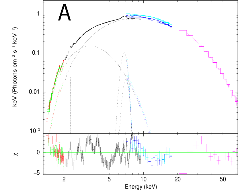
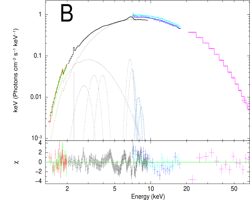
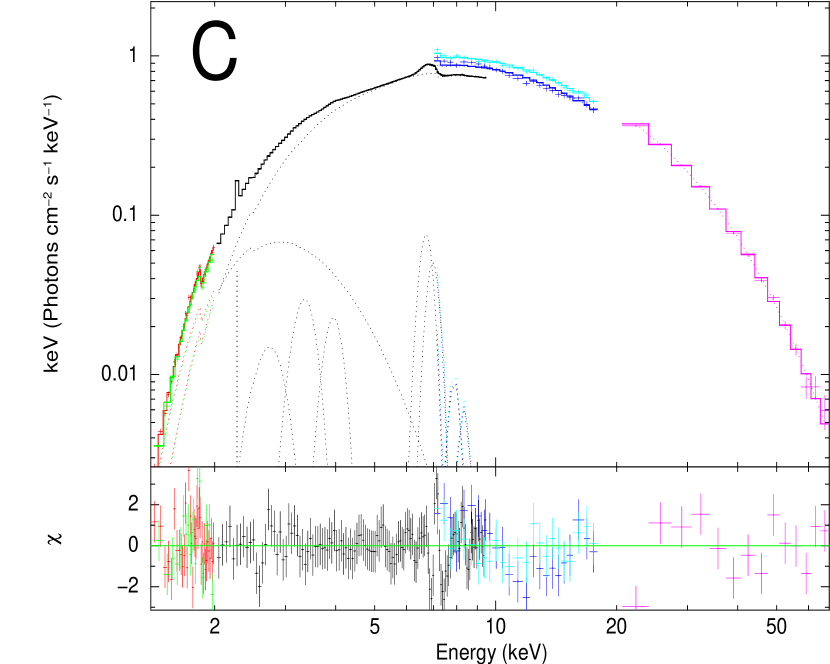
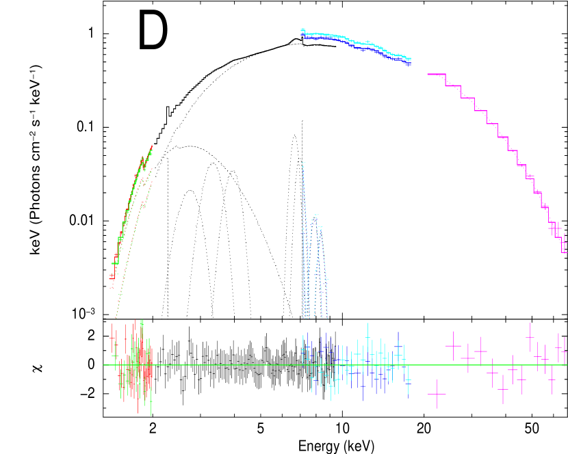
Figure 9: Data, best-fit unfolded models ($E\times f(E)$ representation) and residuals in units of $\sigma$ for a model composed of an accretion disk component and a thermal Comptonization model. RGSo1 data in red, RGSo2 data in green, EPIC/pn (full spectrum) data in black, JEMX1 data in blue, JEMX2 data in light blue, ISGRI data in magenta. RGS data graphically re-binned for clarity. Panel A: addition of two moderately broadened emission Gaussian lines in the iron range; panel B: addition of a set of highly ionized emission lines; panel C: addition of a gabs at $\sim$ 5 keV. panel D: addition of two other gabs harmonics at $\sim$ 10 and $\sim$ 15 keV and of a zero-width line at 7.11 keV.

Table 1: Spectral fitting results for the model disk+nthcomp. Continuum and cyclotron line parameters. Errors given at $\Delta\chi^{2}\,=\,2.706$ (90% confidence for the single interesting parameter).

Parameter (Units)	Value
N${}_{\textrm{H}}$ (1022 cm-2)	6.3$\pm$0.1
$\Gamma$	1.96$\pm$0.09
kTe (keV)	6.75$\pm$0.26
kTbb (keV)	1.80$\pm$0.08
Norm.a	0.11${}_{-0.01}^{+0.04}$
kTdisk (keV)	0.54${}_{-0.07}^{+0.11}$
Inner disk radius Rez (Rg)	27${}_{-7}^{+18}$
E1 (keV)	5.31${}_{-0.14}^{+0.09}$
W1 (keV)	0.39${}_{-0.09}^{+0.18}$
D1 ($\times$ 10-2)	2.9${}_{-0.1}^{+0.4}$
E2 (keV)	11.4${}_{-0.4}^{+1.0}$
W2 (keV)	0.78b
D2 ($\times$ 10-2)	22$\pm$10
E3 (keV)	15${}_{-1.0}^{+2.0}$
W3 (keV)	1.17c
D3 ($\times$ 10-2)	32${}_{-15}^{+25}$
Constant RGSo1/PN	1.13$\pm$0.02
Constant RGSo2/PN	1.08$\pm$0.02
Constant JEMX1/PN	1.18$\pm$0.02
Constant JEMX2/PN	1.32$\pm$0.02
Constant ISGRI/PN	1.33$\pm$0.10
$\chi^{2}_{red}$ (dof)	1.00 (515)
a nthcomp normalization, unity at 1 keV for a norm of 1.
b Parameter tied to 2 $\times$ W1.
c Parameter tied to 3 $\times$ W1.

Table 2: Emission lines in the spectrum of GRO J1744-28. Errors given at $\Delta\chi^{2}\,=\,2.706$ (90% confidence for the single interesting parameter).

Ion (Transitiona)	Elab	Eobs	Width	Fluxb	EQWc
	keV	keV	eV	(10-4)	eV
K$\alpha$ S xvi	2.62	2.65${}_{-0.03}^{+0.04}$	=Ca xix	160${}_{-10}^{+40}$	60${}_{-10}^{+20}$
K$\alpha$ Ar xviii	3.32	3.28${}_{-0.02}^{+0.03}$	=Ca xix	150${}_{-10}^{+40}$	70$\pm$5
K$\alpha$ Ca xix	3.90	3.91$\pm$0.02	240$\pm$10	82${}_{-17}^{+10}$	44$\pm$6
K$\alpha$ Fe xxv	6.70	6.69$\pm$0.04	210${}_{-40}^{+20}$	67${}_{-11}^{+30}$	55$\pm$15
K$\alpha$ Fe xxvi	6.97	6.96$\pm$0.07	=Fe xxv	40${}_{-22}^{+12}$	30$\pm$10
K$\beta$ Fe xxv	7.88	7.88d	=Fe xxv	7.9${}_{-3.2}^{+4.9}$	7.4$\pm$2.5
K$\beta$ Fe xxvi	8.25	8.25d	=Fe xxv	5.1${}_{-1.3}^{+1.7}$	5.1${}_{-1.0}^{+2.3}$
systematic		2.264$\pm$0.004	0d	60$\pm$6	18$\pm$3
systematic		7.11${}_{-0.1}^{+0.2}$	0d	12${}_{-1}^{+2}$	9.4$\pm$2.4
a Rest-frame energies from Verner et al. (1996).
b Total area of the Gaussian (absolute value), in units of photons/cm2/s.
c Line equivalent width.
d Frozen parameter.

3.4 Modelling the highly-ionized features with a reflection component

We have shown in the previous section as a possible interpretation for the large deviations from the continuum shape can be due to the presence of large, moderately deep, absorption features that we interpreted as signs of CRSFs. We have also shown a complex pattern of local emission features, moderately broadened, and compatible with a set of highly ionized transitions from a photo-ionized environment. We investigate the characteristics of the line emission spectrum applying a self-consistent and physically motivated scenario for this set of local features. Excluding a possible origin in a thermal environment, that would require unrealistic MeV temperature, we make the hypothesis that this set of lines is due to reflection in an accretion disk that is still relatively close to the NS to produce appreciable dynamical and relativistic broadening.

To this aim, we slightly changed the continuum shape in order to self-consistently incorporate the reflection component, adopting the reflection model relxill (see details in Dauser et al. 2010; García et al. 2014). This model assumes as incident continuum a cut-off power-law and it correctly takes into-account the angle-dependent reflection pattern. The reflection component is calculated only down to values of photon-index, $\Gamma$, of 1.4 and cut-off energy of 20 keV; such values are sensibly different from the continuum parameters that we found, however, because the reflection component is mainly a contributor in the iron range (fluorescence lines), we retain the model still a reasonable and satisfactory approximation of the true reflection pattern. We left as free parameter the inner disk radius (R_in), the inclination angle and the emissivity index ($\epsilon$). The outer disk radius was held fixed at 1000 R_g, and the spin parameter $a$=0. The other free parameters of this component are the ionization parameter (log($\xi$)), the reflection fraction ($Refl.\leavevmode\nobreak\ fr.$) and the iron abundance relative to the solar value ($A_{Fe}$).

We tested our constraints on the widths of the CRSFs, but we found the widths of the first and second harmonic to be significantly different from 2 $\times$ W₁ and 3 $\times$ W₁, and, to obtain a satisfactory fit, we left the CRSFs widths free to vary. We note that the two harmonics become statistically more necessary with respect to the continuum model of Table 1 (both features detected at $\sim$ 6.8 $\sigma$, but the single harmonics are detected at $\sim$ 3 $\sigma$ level), implying a certain model-dependent detection. We tested the presence of the softer disk component, left free to vary energy and normalization of the 2.22 keV instrumental feature. The best-fitting model has a final reduced chi-squared of 1.32 (526 dof), it describes quite satisfactorily the residual pattern in the iron range although we noted (left panel of Fig.10) that some residuals still persisted at the energies corresponding to the K$\alpha$ Si xvi, Ar xviii, Ca xix and Ca xx emission lines. To model the larger intensities suggested by these residuals, we used blurred relativistic profiles (relconv model) for the non-iron highly ionized emission lines, setting the blurring parameters (inner and outer disk radius, inclination angle and emissivity profile index of the relconv component) to be tied to the parameters of the relxill model. We found that the broadened line at $\sim$ 3.9 keV, identified with the K$\alpha$ Ca xix transition in Table 2, is much better modelled with a combination of He- and H-like calcium emission lines. We found that the energies of the K$\alpha$ Ar xviii, Ca xix and Ca xx are consistent with the expected rest-frame values, but the position of the S xvi line is found at higher energies (2.73 $\pm$ 0.02 keV), however setting the line energy at 2.62 keV still gives a lower limit on the normalization higher than zero. We calculated the errors on the line normalizations freezing the line energies at the laboratory frame values, obtaining normalization values significantly lower than the values reported in Table 2 and physically more consistent with the expected widths implied by the blurring parameters of the fluorescence iron transitions (Table 3).

Finally, we added a zero-width line at $\sim$ 7.11 keV, finding best-fitting position and normalization consistent with the values reported in Table 2, and obtaining a final best-fit reduced $\chi^{2}$ of 1.025 (519 dof) and a satisfactory pattern of residuals as shown in Fig. 10. In Fig. 11, we show the broadband data/model ratio for a best-fit continuum without emission/absorption features (panel A); for the best-fitting model of Table 3 when the reflection fraction is set to zero (panel B); when the depth of the fundamental cyclotron line is set to zero (panel C); when the depths of the two harmonics are set to zero (panel D).

During the fitting procedure we noted that the inner disk radius, R_in, of the reflection component becomes rather unconstrained by the fit because of a strong correlation with the other smearing spectral parameters (i.e. inclination angle and $\epsilon$). Fixing the inclination angle to 18^∘, 22^∘, and 25^∘, we obtained a lower limit on R_in of 90 R_g, 80 R_g, and 70 R_g, respectively. For higher values of the inclination angle R_in is not constrained. If the value of the $\epsilon$ parameter is frozen to 3 (a value that would correspond to an isotropic point-like irradiating source), we obtained a lower limit for R_in of $\sim$ 100 R_g; if both the inclination is fixed to 22^∘ (upper limit based on the calculations from Rappaport & Joss 1997, Table 3) and $\epsilon$ = 3, then the lower limit for R_in is 120 R_g.

In Table 3, first column, we report the best-fitting results with R_in fixed to a reference value of 100 R_g. Finally, we note that if no systematic error is assumed for the EPIC/pn data, then a strict lower limit on R_in is derived at $\sim$ 60 R_g (Table 3, second column). We obtained similar results adopting the EPIC/pn spectrum without the three central columns (Table 3, third column).

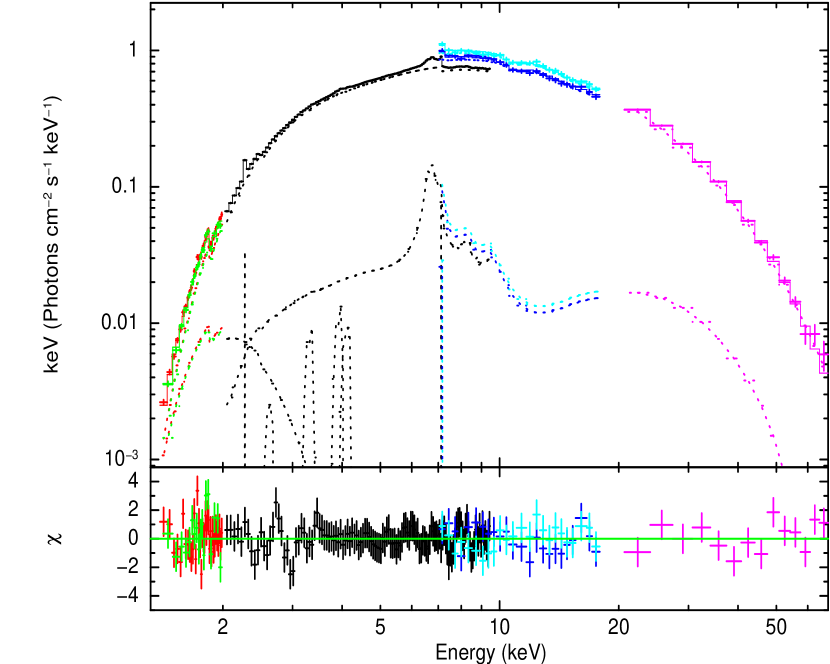
Figure 10: Data, unfolded model with additive components (upper panel) and residuals in units of $\sigma$ (lower panel) using the disk+relxill model1 (Table 3) and a set of ionized emission lines with common blurring parameters.

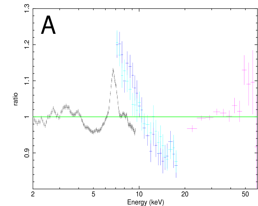
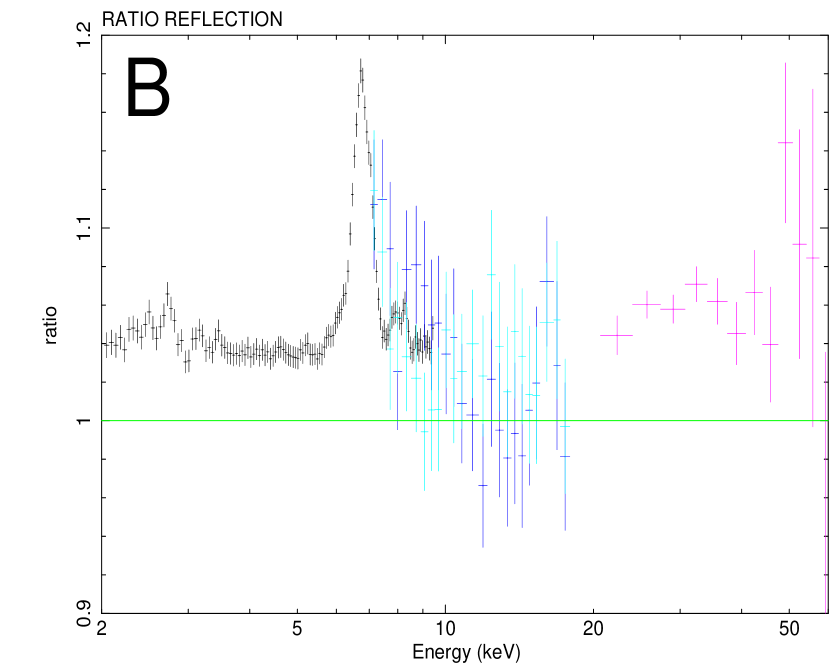
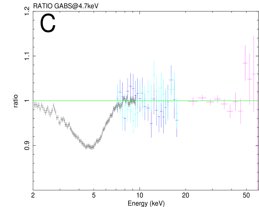
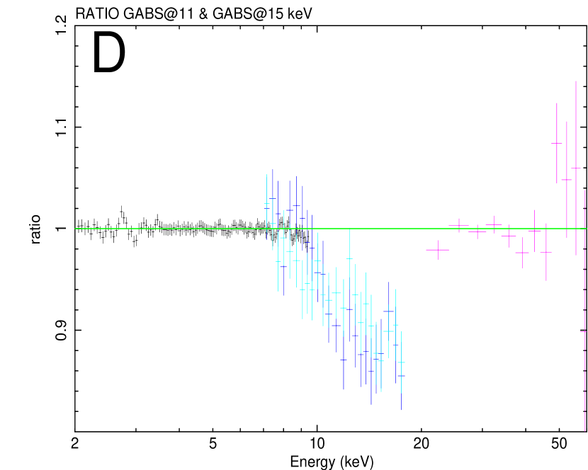
Figure 11: 2-60 keV data/model ratios: for a best-fitting continuum without reflection and gabs (panel A), for the best-fitting continuum of Table 3 with $Refl.\,fr.$ set to 0 (panel B); for the best-fitting continuum of Table 3 with D₁ set to 0; for the best-fitting continuum of Table 3 with D₂ and D₃ set to 0.

Differently from the nthcomp Comptonization model, the relxill continuum has no low-energy roll-over, implying a higher flux of this component in the softest X-ray band. This affected the determination of the disk emission, and we obtained a shift of the ezdiskbb temperature to lower values and a higher value for the disk inner radius (R_ez $\sim$ 90 R_g). We found that the reflection component requires a high metallicity, where iron over-abundance is $\sim$10 the solar value. Also the emission lines from the highly ionized transitions of Si/Ar/Ca were not fully well fitted by the broadband reflection model and the residuals strongly required more flux at the line energies that we interpreted as an indication of possible higher metal abundance. The companion star of GRO J1744-28 is an evolved giant (Gosling et al. 2007) whose external layers are probably rich in the ejecta of the supernova explosion that generated GRO J1744-28 and a high level of metallicity in the accretion flow could be expected.

The best-fitting parameters and associated errors are shown in first column of Table 3, while in the second and third columns of the same table, we comparatively show the two best-fitting models using the EPIC/pn data without any systematic error (second column), and the EPIC/pn spectrum extracted from the wings of the PSF (excising the three hottest RAWX columns) and no systematic error (third column). The range of best-fitting values and associated errors is useful to comparatively visualize the impact of the assumptions based on the choice to assign a systematic error to the EPIC/pn data and the impact of possible residual pile-up.

Table 3: Best-fitting parameters and errors for models using a self-consistent reflection component to fit the highly ionized emission lines. In the first column we assigned to the EPIC/pn channel a systematic error of 0.5%, in the second column the EPIC/pn spectrum has no systematic error, in the third column we used the EPIC/pn spectrum obtained by excising the PSF after removing the three central columns. Errors given at $\Delta\chi^{2}\,=\,2.706$ (90% confidence for the single interesting parameter).

	0.5% sys.	No sys.error	3 cols
N${}_{\textrm{H}}$ (1022 cm-2)	6.4$\pm$0.3	6.15$\pm$0.15	6.2${}_{-0.3}^{+0.2}$
$\Gamma$	0.33${}_{-0.07}^{+0.12}$	0.295$\pm$0.015	0.49$\pm$0.07
Norm.a	0.45$\pm$0.06	0.42$\pm$0.01	0.55${}_{-0.06}^{+0.04}$
Ecut (keV)	8.56$\pm$0.15	8.48$\pm$0.10	8.94${}_{-0.16}^{+0.11}$
kTdisk (KeV)	0.29$\pm$0.04	0.30$\pm$0.02	0.28$\pm$0.02
Rez (Rg)	90${}^{+100}_{-50}$	65${}_{-15}^{+50}$	100${}_{-40}^{+35}$
E1 (keV)	4.68$\pm$0.05	4.75${}_{-0.02}^{+0.03}$	4.59$\pm$0.06
W1 (keV)	0.68$\pm$0.08	1.02$\pm$0.05	0.84$\pm$0.07
D1 ($\times$ 10-2)	8.7$\pm$0.2	22$\pm$3	16$\pm$4
E2 (keV)	10.4$\pm$0.10	11.4$\pm$0.08	9.43$\pm$0.09
W2 (keV)	0.66$\pm$0.10	1.0$\pm$0.4	0.94${}_{-0.08}^{+0.13}$
D2 ($\times$ 10-2)	14$\pm$9	24$\pm$15	25$\pm$7
E3 (keV)	15.8${}_{-0.7}^{+1.3}$	16.0$\pm$0.07	15.4$\pm$0.7
W3 (keV)	2.6${}_{-0.9}^{+0.7}$	2.3$\pm$0.7	2.6$\pm$0.8
D3 ($\times$ 10-2)	90$\pm$30	93$\pm$22	95$\pm$25
$\epsilon$ (emissivity)	1.5${}_{-1.5}^{+2.0}$	1.1${}_{-0.9}^{+1.2}$	2.3${}_{-0.8}^{+1.2}$
Inclination (deg)	28${}_{-10}^{+20}$	28$\pm$4	23${}_{-4}^{+10}$
Rin (Rg)	100b	$>$60	100b
Relxill Log($\xi$)	3.09$\pm$0.02	3.09$\pm$0.02	3.1$\pm$0.03
Relxill $A_{Fe}$	$>$8c	$>$9c	$>$7c
Relxill $Refl.\leavevmode\nobreak\ fr.$ (10-2)	5.3$\pm$0.4	5.3${}_{-0.2}^{+0.7}$	7.6${}_{-1.8}^{+1.2}$
S xvi  norm.d	7$\pm$5	5.6$\pm$1.9	4.9$\pm$3.9
Ar xviii  norm.d	8${}_{-4}^{+2}$	7.9$\pm$1.8	7.3$\pm$2.5
Ca xix  norm.d	8${}_{-3}^{+2}$	7.3$\pm$1.3	6.2$\pm$2.2
Ca xx  norm.d	6$\pm$3	5.4$\pm$1.3	7.7$\pm$2.0
C1 PN/RGSo1	1.15$\pm$0.02	1.16$\pm$0.01	1.07$\pm$0.02
C2 PN/RGSo2	1.02$\pm$0.03	1.10$\pm$0.02	1.02$\pm$0.02
C3 PN/JEMX1	1.19$\pm$0.02	1.18$\pm$0.02	1.36$\pm$0.02
C4 PN/JEMX2	1.32$\pm$0.02	1.32$\pm$0.02	1.52$\pm$0.02
C5 PN/ISGRI	1.20$\pm$0.03	1.16$\pm$0.03	1.41$\pm$0.05
$\chi^{2}_{red}$ (dof)	1.025 (519)	1.408 (519)	1.284 (519)
a In units of photons keV-1 cm-2 s-1 at 1 keV.
b Frozen parameter during fitting search.
c Hard limit for this parameter set to 10.
d Line normalization in units of 10-4 photons cm-2 s-1 in the line.

3.5 The pulsed fraction in the iron region: comparison with best-fitting models

We have shown in Sect. 2.1 that there is a clear drop in the pulsed fraction in the iron region of the spectrum (see Fig. 5) and that the shape of the drop is consistent with a broad Gaussian profile. Such drop has been also noted in Nishiuchi et al. (1999), who proposed its origin in the not-pulsed flux of a relativistically smeared iron line. We have shown that the large iron residuals can be interpreted as reflection from a truncated disk and we establish here if the shape and strength of the residuals of Fig. 5 are consistent with this origin. To this aim, we divided the energy spectral range in bins of 100 eV width from 5.5 keV to 7.5 keV. We calculate for each channel the observed flux of the reflection component, relxill, and of the reflection component according to the best-fitting model of Table. 3. We calculated the not-pulsed $excess$ flux ($F_{ex}$) for the amplitude versus energy plot using a best-fitting third-order polynomial function fit to the pulsed fraction outside the 5.5–7.5 keV range as explained in Sect. 2.2, according to the following expression:

$$F_{ex}=\left(\frac{f_{exp}}{f_{obs}}-1\right)\times F_{tot}$$ (4)

where $f_{exp}$ is the value of the $expected$ pulse fraction in that energy bin from the best-fitting function, $f_{obs}$ is the observed pulsed fraction, and $F_{tot}$ is the continuum flux per bin. In Fig. 12, we show the results of this procedure. We found that the not-pulsed flux excess is in reasonable agreement with the flux of the reflection component.

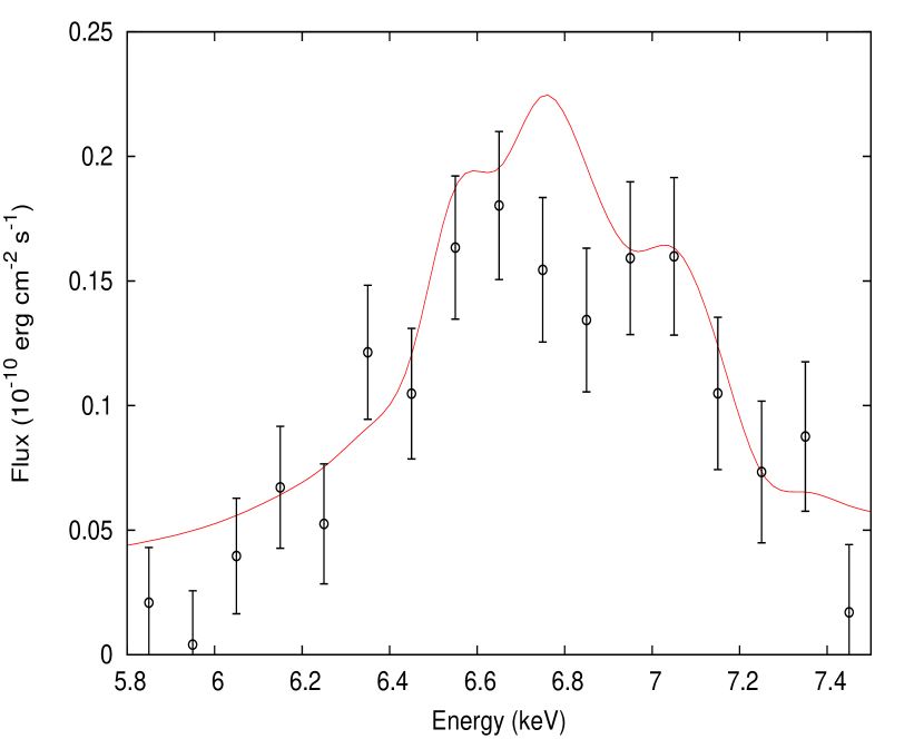
Figure 12: Red line: the reflection component flux according to the best-fit model of Table 3. Black data: excess flux from the amplitude fraction according to Eq. 4.

4 Pulse-phase resolved spectroscopy

Based on the best time-averaged pulse period during the persistent emission, we extracted ten pulse-resolved spectra, equally phase-spaced, to study the spectral evolution as a function of the spin phase. We used only data from the EPIC/pn instrument in the 2.0–9.5 keV range. To get a preliminary idea of the spectral changes, we first plotted the count difference between the time-averaged spectrum and the phase-selected spectrum as a function of the energy channel. The result of this operation is shown in the heat map of Fig.13, where no evident substructure is visible, implying that most of the spectral changes is due to a slowly changing slope of the overall continuum. To fit the spin-resolved spectra we adopted the best-fitting model of Table 3 and we found a global acceptable fit (reduced $\chi^{2}$ 1287/1241) by setting the following parameters free to vary: the photon index ($\Gamma$), the normalization of the relxill component, and the reflection fraction. The remaining parameters of the fit were kept fixed to the best-fitting values of the pulse-averaged spectrum (Table 3).

In Fig. 14, we show the variation of the photon-index, reflection fraction and absorbed flux as a function of the spin phase, all following the smooth sinusoidal trend of the pulsed flux. We clearly observe that the lowest value of the photon-index is found in correspondence with the pulse maximum, while the highest reflection fraction is at the pulse minimum. Because the reflection fraction is the ratio between the reflected and the direct, primary flux, this result suggests that the reflected flux does not sensibly depend on the pulse phase and we verified this by calculating the reflected flux for each phase-selected spectrum, finding it constant within a $\sim$ 5% relative uncertainty. We did not detect statistically significant variations of the fundamental cyclotron line parameters along the pulse phase.

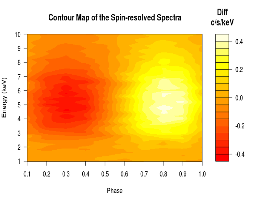
Figure 13: Heat map for the EPIC/pn spin-resolved spectra. We plot on the y-axis the count/s/keV difference with respect to the time-averaged spectrum.

Figure 14: Best-fitting parameters 1 $\sigma$ errors for the ten phase-resolved spectra. From top to bottom: relxill 0.5–10 keV unabsorbed flux in units of 10^-8 erg cm^-2 s^-1, photon-index, and reflection fraction.

5 Discussion

In this paper we presented a complete analysis of the broadband (1.3–70 keV) spectral characteristics of the persistent emission of the bursting pulsar GRO J1744-28 based on a long continuous XMM-Newton observation and on the hard X-ray coverage provided by two of the instruments on board of $INTEGRAL$ (JEMX and ISGRI).

The EPIC/pn spectrum is, however, affected by some level of uncertainty, because of the high registered count rate causing instrumental spectral distortions and shifts in the energy scale (i.e. charge transfer inefficiency and X-ray loading, see Pintore et al. 2014) and by some level of photon pile-up. To process the EPIC/pn data we adopted the RDPHA pipeline as suggested by the EPIC/pn hardware team, and we obtained our best-fitting results considering both an excised PSF and the total PSF (full spectrum, see Table 3). The main spectral differences in the two spectra affect the determination of the power-law photon index, the cut-off energy, and the depth of the first harmonic, which resulted each other not compatible. Moreover, the EPIC/pn spectrum is according to us affected by two other (possible) instrumental artefacts: a narrow emission line at $\sim$ 2.2 keV, observed in the spectra of bright sources either in emission or in absorption (Hiemstra et al. 2011; Pintore et al. 2014), due to the strong effective area derivative of the Au-M edge and a narrow line at 7.11 keV, where there is a physical spectral discontinuity due to the sharp neutral iron edge. The RDPHA method assigns a $\sim$ 20 eV uncertainty in the photon energy scale reconstruction, and the appearance of such narrow feature could be caused by a slight mismatch in the energy scale reconstruction of photons in this band.

However, despite these caveats, the overall picture and interpretation of the main physical processes producing the X-ray spectrum remains quite solid, because it was found not to sensibly depend on these instrumental uncertainties (Table 3).

5.1 Continuum emission and cyclotron lines

The X-ray continuum spectrum of an accreting pulsar is governed by different physical process that are all sensible to the local condition of the accreting plasma and to the geometry and strength of the NS magnetic field. Soft photons produced by bremsstrahlung, synchrotron and thermal, black-body, emission are Compton up-scattered to higher energies either by the energetic, free-falling, electrons (bulk-motion Comptonization) or through thermal Comptonization. X-ray pulsars accreting above the critical luminosity ($L_{crit}$ $\approx$ 3 $\times$ 10³⁶ erg s^-1 Basko & Sunyaev 1976; Becker & Wolff 2005) have a radiative shock, formed and sustained by the Eddington radiation pressure, and a significant part of the scattering process is due to thermal Comptonization. For sources below the critical luminosity, bulk-motion (or fist-order Fermi energization) dominates. Sources in this latter category show steeper spectra ($\Gamma>$ 2), whereas sources of the former class appear flatter ($\Gamma<$ 2, Becker & Wolff (2007)).

Because of the complexity and non-linearity of all these processes, the pulsar spectra have usually been fitted with phenomenological models, that, however, provided in most cases a statistical adequate description of the data, and a general common frame for comparing the spectra of different sources and detect, even very broad local absorption/emission features (Heindl et al. 2004). We found that the broadband spectrum GRO J1744-28, however, cannot be described in terms of simple power-law models (whatever the prescription for the exponential cut-off), or combinations of black-body and cut-off power-laws, that are more typical for bright un-magnetized accreting NSs. We observed a common trend of residuals, extending in the 4.0–10.0 keV range, giving rise to a spectral curvature that can be satisfactorily accounted by a set of broad features in absorption at the edges of the iron K$\alpha$ region, together with a set of moderately broadened features in emission, that can be satisfactorily described with a self-consistent reflection component, smeared by dynamical and relativistic effects produced at the inner edge of a truncated disk. The presence of these features is statistically required independently from the adopted continuum. We have modelled it first with the sum of a soft thermal disk emission and a thermal Comptonization model (nthcomp), that has two main parameters that determine the cut-off, high-energy, roll-over (the electron temperature and the cloud optical depth, related to the $\Gamma$ parameter). We note here that we obtained very similar results, in terms of $\chi^{2}$ and spectral parameters for the local emission/absorption features, using a power-law with a highecut cut-off, a model widely adopted for describing the hard spectra of X-ray pulsars. The addition of an other continuum component (as a black-body emission) resulted in thermal temperatures that closely followed the shape of the nthcomp soft seed-photon temperature, and we concluded that the nthcomp encloses all the characteristics of the most commonly models used in the literature to fit the spectra of bright X-ray pulsars.

In Sect. 3.4 we showed results from a simpler continuum made with a cut-off power-law (relxill model), a softer thermal disk emission (ezdiskbb), and a broadband reflection component. The reflected spectrum is also an important continuum contributor, through continuum Thomson scattering and bremsstrahlung emission, and significant changes in the best-fitting parameters of the other local features in absorption were expected (compare Table 1 and Table 3). It is clear that the modelling of the underneath continuum is more important than the statistical uncertainties from the best-fitting modelling, although the general picture of the cyclotron features appears quite solid. The uncertainty on the cyclotron fundamental energy is of the order of 6%, the width of 25%, whereas the depth is the most sensible parameter, due to the strong correlation with the general shape of the fluorescence iron line.

If we use the best-fitting parameters from Table 3 for the fundamental cyclotron line energy (E₁ = 4.7 keV), we can derive the magnetic field of the NS using Eq. 2, leading to a magnetic dipole field of (5.27 $\pm$ 0.06) $\times$ 10¹¹ G (magnetic dipole moment $\mu$ = 5.27 $\times$ 10²⁹ G cm³), assuming the CRSF is formed at the surface of the NS (gravitational red-shift $z$ = 0.3).

This estimate allows to constrain the magnetospheric radius ($R_{M}$), where the ram pressure of the accretion flow is balanced by the magnetic pressure, according to the formula (Frank et al. 2002):

$$R_{M}=2.9\times 10^{8}\kappa_{m}M_{NS}^{1/7}R_{6}^{-2/7}L_{37}^{-2/7}\mu_{30}^{4/7}\quad\textrm{cm}$$ (5)

where $\kappa_{m}$ is a coefficient related to the accretion flow geometry (1 for isotropic radial accretion), $M_{NS}$ is the NS mass in units of $M_{\odot}$, $R_{6}$ is the NS radius in units of 10⁶ cm, $L_{37}$ is the source luminosity in units of 10³⁷ erg s^-1, and $\mu_{30}$ is the magnetic dipole moment in units of 10³⁰ G cm³. From our B estimate, the bolometric luminosity derived by extrapolating the observed flux, assuming isotropic emission, and classical values for the NS mass and radius (1.4 M_⊙, 10⁶ cm radius), we derive a value of $R_{M}$ $\simeq$ 10⁸ $\times\kappa_{m}$ cm. The co-rotation radius for a NS of period P_spin is

$$R_{\Omega}=\left(\frac{GMP^{2}_{spin}}{4\pi^{2}}\right)^{1/3}$$ (6)

and corresponds for GRO J1744-28 to 10⁸ cm. A value of $\kappa_{m}$ close to 1 (isotropic accretion) would imply that the NS is accreting at the spin equilibrium. However, we derived from the best-fitting parameters of the disk emission and of the reflection component an inner disk radius lower limit closer to a value of 2 $\times$ 10⁷ cm, that sets the $\kappa_{m}$ lower limit value at $\sim$ 0.2, that is in agreement with the value $\sim$ 0.2 reported for low B-field pulsars in Burderi et al. (2002), and not unrealistically lower than a more recent estimate of 0.5 found by Long et al. (2005). We also note that, as discussed by Bozzo et al. (2009), the expected value of this parameter is affected by large uncertainties due to the different theoretical prescriptions for the magnetospheric radius published so far.

We found that the width of the fundamental CSRF is 15–20% the value of the energy position, and this is in line with what observed in similar other accreting pulsars (see Fig. 5 in Heindl et al. 2004). Adopting the classical formulation for the thermal broadening in a plasma with electron temperature $kT_{e}$ (Meszaros & Nagel 1985):

$$\left(\frac{\Delta E}{E}\right)_{FWHM}=\left(\frac{8\textrm{ln}2\quad kT_{e}}{m_{e}c^{2}}\right)^{1/2}\textrm{cos}\theta$$ (7)

assuming an angle $\theta$ $\sim$ 20^∘, we can derive an electron temperature of $\sim$ 11 keV, which is quite close to the cut-off energy of the broadband spectrum, estimated at $\sim$ 8.6 keV. From the spin-resolved analysis, we found that the fundamental cyclotron feature did not show any statistical significant correlation with the pulsed emission. Degenaar et al. (2014) noted in the $Chandra$/HETGS observation of GRO J1744-28 an unidentified absorption line at $\sim$ 5.11 keV that was tentatively associated with a cyclotron absorption feature, though the line width could not be constrained and it was kept fixed to 10 eV in the fit. Because the energy and the width of the fundamental cyclotron line as derived by our analysis of the EPIC/pn data (Table 3) points towards a significantly broader feature, we retain that these two detections are not related.

We found a suggestive, but statistically weak, hint of two cyclotron harmonics at $\sim$ 11 keV and $\sim$ 15 keV. We note that Younes et al. (2015) reported also a broad dip in the $NuSTAR$ spectrum of this source at $\sim$ 10 keV, whose shape resembles the one shown in the $INTEGRAL$/JEMX data. The widths and depths of these two features could not be independently determined, because the features are broad and they spectrally overlap. Moreover, we noted a certain dependence based on the assumptions for the continuum and for the systematics that affect the inter-calibration of the different instruments that were used to constrain these shapes. Notwithstanding these limitations, the energies of the first and second harmonics were always found close to the expected harmonic ratios 1:2 and 1:3 (for a fundamental line at $\sim$ 4.7 keV), and GRO J1744-28 would be, after 4U 0115+64 (Müller et al. 2013, CRSF fundamental at 14 keV) and V 0332+53 (Pottschmidt et al. 2005, CRSF fundamental at 26 keV), the third X-ray pulsar to show a second harmonic in its spectrum. The slight discrepancy in the harmonic ratios (2.2 and 3.3 for the first and second harmonic, respectively) has been observed also in other X-ray pulsars, and it has been shown to be dependant on the accretion rate as discussed in Nakajima et al. (2010). We found that the two harmonics have larger depths with respect to the fundamental, as reported in other sources (e.g. for X0115+63, Santangelo et al. 1999), an observational fact explained through the two-photon process (Alexander & Meszaros 1991). Because these features lie outside the EPIC/pn band, we could not track parameter variations with respect to the spin-phase.

5.2 The highly ionized reflection component: GRO J1744-28 between the LMXB and the HMXB class

The set of highly ionized feature is satisfactorily compatible with a reflection spectrum from a cold disk truncate at large distance from the NS. The inner disk radius estimate is correlated with the values of the other smearing parameters, but for realistic values of both inclination angle ($\sim$ 22 deg) and index of the emissivity law profile ($\epsilon$ = 3), a lower limit value on R_in is obtained at 120 R_g. The temperature and the luminosity of the disk continuum component was found compatible with this estimate. Differently from Nishiuchi et al. (1999), we do not find evidence of extreme red wings, that would imply low inner disk radii, and our estimate is rather close to an independent estimate based on the iron line shape observed in the $Chandra$ observation analysed by Degenaar et al. (2014).

The presence of reflection components in highly magnetized accreting pulsars has been usually neglected, because of the large distance of the inner disk radius (if present) and expected low reflection fraction. Ballantyne et al. (2012) first proposed a set of self-consistent reflection tables and showed that moderately broad emission features could be signatures of such component as in the case of the accreting pulsar LMC X-4. In that case however blurring parameters derived from best-fitting did not provide physically consistent results, as the derived inner radii were too low compared with the expected disk truncation radius at the magnetosphere. On the contrary, for weakly magnetized accreting X-ray pulsars the detection of reflection components has been already established in a considerable amount of cases. A relativistic iron line profile has been first reported for SAX J1808.4-3658, where the blurring parameters were found in line with the expectations (Papitto et al. 2009), and later also for IGR J17511-3057 (Papitto et al. 2010), IGR J17480-2446 (Miller et al. 2011) and in HETE J1900.1-2455 (Papitto et al. 2013). In the above-mentioned cases the inner disk radii were constrained in the range 20–40 R_g and were consistent with the possible magneto-spheric radii derived from the study of spin timing, whereas in non-pulsating accreting neutron stars significantly lower values were derived (6–15 R_g, see Cackett et al. 2010).

We derived an inclination angle between 18^∘ and 48^∘, that is within the range of values for the system according to the possible evolutionary histories of the system (Rappaport & Joss 1997). From the X-ray mass function of GRO J1744-28 (Finger et al. 1996), we thus derive an upper limit on the companion mass between 0.23 M_⊙ and 0.27 M_⊙, for a 1.4 and 1.8 M_⊙ NS mass, respectively. This range encompasses the most probable value (0.24 M_⊙) indicated for the present companion mass by Rappaport & Joss (1997).

The reflected component has a high ionization degree (log$\xi$ $\sim$ 3.1) as expected from the presence of H- and He-like emission lines, and from the distance of the inner disk radius and bolometric source luminosity, we can estimate the reflector electron density $n_{e}$ = $L_{bol}/(r^{2}\xi)$ $\sim$ 3 $\times$ 10²⁰ cm^-3.

6 Conclusions

We presented results from the spectral analysis of the broadband spectrum of the bursting pulsar GRO J1744-28. Using $XMM-Newton/INTEGRAL$ data we covered the 1.3–70 keV energy range, when the source was accreting near the Eddington limit for a 1.4 M_⊙ NS. Independently from the adopted continuum, we found in the spectrum a moderately broadened absorption feature in the range 4.6–5.3 keV and a set of moderately broadened emission features. We interpreted this absorption dip in terms of a cyclotron resonant scattering feature and we also found suggestive evidence of two other absorption features close to the energies expected for the first and second harmonic. From this interpretation, we derived an estimation of the GRO J1744-28 pulsar magnetic field, 5.27 $\pm$ 0.06 $\times$ 10¹¹ G.
We located the region responsible for the moderately broadened emission lines outside the pulsar magnetosphere, in a reflecting, accretion disk. The study of the pulse amplitude fraction and the spin-resolved spectra indicated that the iron complex in emission is not pulsed and its flux is not phase-dependent. We found that the disk surface is highly photo-ionized, with log($\xi$) $\sim$ 3.1, with a metal over-abundance of a factor $\sim$ 10 and truncated at a distance of $\gtrsim$ 100 R_g, where dynamical effects, caused by the high velocities of matter in the disk, are still important. The spectrum is also characterized by soft disk emission, whose truncation radius results compatible with the estimate from the reflected component. These two independent, but converging, constraints allowed us to estimate the Alfvén efficiency parameter for disk-accretion, close to 0.2. The lower limit on the inclination angle of the disk is 18^∘ and compatible with independent estimates on the possible evolutionary history of the system (Rappaport & Joss 1997).

7 Acknowledgements

We are specially grateful to N. Schartel, who made possible this ToO observation through the Director Discretionary Time and all the XMM-Newton team who performed and supported this observation.
The High-Energy Astrophysics Group of Palermo acknowledges support from the Fondo Finalizzato alla Ricerca (FFR) 2012/13, project N. 2012-ATE-0390, founded by the University of Palermo.
A.  R.  gratefully acknowledges the Sardinia Regional Government for the financial support (P. O.  R. Sardegna F.S.E. Operational Programme of the Autonomous Region of Sardinia, European Social Fund 2007-2013 - Axis IV Human Resources, Objective l.3, Line of Activity l.3.1).

References

- Alexander & Meszaros (1991) Alexander S. G., Meszaros P., 1991, ApJ, 372, 565
- Anders & Ebihara (1982) Anders E., Ebihara M., 1982, Geochim. Cosmochim. Acta, 46, 2363
- Anders & Grevesse (1989) Anders E., Grevesse N., 1989, Geochim. Cosmochim. Acta, 53, 197
- Augusteijn et al. (1997) Augusteijn T., Greiner J., Kouveliotou C., van Paradijs J., Lidman C., Blanco P., Fishman G. J., Briggs M. S., Kommers J., Rutledge R., Lewin W. H. G., Henden A. A., Luginbuhl C. B., Vrba F. J., Hurley K., 1997, ApJ, 486, 1013
- Ballantyne et al. (2012) Ballantyne D. R., Purvis J. D., Strausbaugh R. G., Hickox R. C., 2012, ApJL, 747, L35
- Basko & Sunyaev (1976) Basko M. M., Sunyaev R. A., 1976, MNRAS, 175, 395
- Becker & Wolff (2005) Becker P. A., Wolff M. T., 2005, ApJ, 630, 465
- Becker & Wolff (2007) Becker P. A., Wolff M. T., 2007, ApJ, 654, 435
- Beri et al. (2014) Beri A., Jain C., Paul B., Raichur H., 2014, MNRAS, 439, 1940
- Bildsten & Brown (1997) Bildsten L., Brown E. F., 1997, ApJ, 477, 897
- Bozzo et al. (2009) Bozzo E., Stella L., Vietri M., Ghosh P., 2009, A&A, 493, 809
- Burderi et al. (2010) Burderi L., Di Salvo T., Riggio A., Papitto A., Iaria R., D’Aì A., Menna M. T., 2010, A&A, 515, A44
- Burderi et al. (2002) Burderi L., Di Salvo T., Stella L., Fiore F., Robba N. R., van der Klis M., Iaria R., Mendez M., Menna M. T., Campana S., Gennaro G., Rebecchi S., Burgay M., 2002, ApJ, 574, 930
- Cackett et al. (2010) Cackett E. M., Miller J. M., Ballantyne D. R., Barret D., Bhattacharyya S., Boutelier M., Miller M. C., Strohmayer T. E., Wijnands R., 2010, ApJ, 720, 205
- Cannizzo (1997) Cannizzo J. K., 1997, ApJ, 482, 178
- Coburn et al. (2002) Coburn W., Heindl W. A., Rothschild R. E., Gruber D. E., Kreykenbohm I., Wilms J., Kretschmar P., Staubert R., 2002, ApJ, 580, 394
- Cui (1997) Cui W., 1997, ApJL, 482, L163
- D’Aì et al. (2010) D’Aì A., di Salvo T., Ballantyne D., Iaria R., Robba N. R., Papitto A., Riggio A., Burderi L., Piraino S., Santangelo A., Matt G., Dovčiak M., Karas V., 2010, A&A, 516, A36
- D’Aì et al. (2014) D’Aì A., Di Salvo T., Iaria R., Riggio A., Burderi L., Sanna A., Pintore F., 2014, The Astronomer’s Telegram, 5858, 1
- Daigne et al. (2002) Daigne F., Goldoni P., Ferrando P., Goldwurm A., Decourchelle A., Warwick R. S., 2002, A&A, 386, 531
- Daumerie et al. (1996) Daumerie P., Kalogera V., Lamb F. K., Psaltis D., 1996, Nature, 382, 141
- Dauser et al. (2010) Dauser T., Wilms J., Reynolds C. S., Brenneman L. W., 2010, MNRAS, 409, 1534
- Degenaar et al. (2014) Degenaar N., Miller J. M., Harrison F. A., Kennea J. A., Kouveliotou C., Younes G., 2014, ApJL, 796, L9
- Degenaar et al. (2012) Degenaar N., Wijnands R., Cackett E. M., Homan J., in’t Zand J. J. M., Kuulkers E., Maccarone T. J., van der Klis M., 2012, A&A, 545, A49
- Finger et al. (2014) Finger M. H., Jenke P. A., Wilson-Hodge C., 2014, The Astronomer’s Telegram, 5810, 1
- Finger et al. (1996) Finger M. H., Koh D. T., Nelson R. W., Prince T. A., Vaughan B. A., Wilson R. B., 1996, Nature, 381, 291
- Frank et al. (2002) Frank J., King A., Raine D. J., 2002, Accretion Power in Astrophysics: Third Edition. Accretion Power in Astrophysics, by Juhan Frank and Andrew King and Derek Raine, pp. 398. ISBN 0521620538. Cambridge, UK: Cambridge University Press, February 2002.
- García et al. (2014) García J., Dauser T., Lohfink A., Kallman T. R., Steiner J. F., McClintock J. E., Brenneman L., Wilms J., Eikmann W., Reynolds C. S., Tombesi F., 2014, ApJ, 782, 76
- Giles et al. (1996) Giles A. B., Swank J. H., Jahoda K., Zhang W., Strohmayer T., Stark M. J., Morgan E. H., 1996, ApJL, 469, L25
- Gosling et al. (2007) Gosling A. J., Bandyopadhyay R. M., Miller-Jones J. C. A., Farrell S. A., 2007, MNRAS, 380, 1511
- Heindl et al. (2004) Heindl W. A., Rothschild R. E., Coburn W., Staubert R., Wilms J., Kreykenbohm I., Kretschmar P., 2004, in Kaaret P., Lamb F. K., Swank J. H., eds, X-ray Timing 2003: Rossi and Beyond Vol. 714 of American Institute of Physics Conference Series, Timing and Spectroscopy of Accreting X-ray Pulsars: the State of Cyclotron Line Studies. pp 323–330
- Hiemstra et al. (2011) Hiemstra B., Méndez M., Done C., Díaz Trigo M., Altamirano D., Casella P., 2011, MNRAS, 411, 137
- Iaria et al. (2013) Iaria R., Di Salvo T., D’Aì A., Burderi L., Mineo T., Riggio A., Papitto A., Robba N. R., 2013, A&A, 549, A33
- Jahoda et al. (1999) Jahoda K., Stark M. J., Strohmayer T. E., Zhang W., Morgan E. H., Fox D., 1999, Nuclear Physics B Proceedings Supplements, 69, 210
- Kouveliotou et al. (1996) Kouveliotou C., van Paradijs J., Fishman G. J., Briggs M. S., Kommers J., Harmon B. A., Meegan C. A., Lewin W. H. G., 1996, Nature, 379, 799
- Krimm et al. (2013) Krimm H. A., Holland S. T., Corbet R. H. D., Pearlman A. B., Romano P., Kennea J. A., Bloom J. S., Barthelmy S. D., Baumgartner W. H., Cummings J. R., Gehrels N., Lien A. Y., Markwardt C. B., Palmer D. M., Sakamoto T., Stamatikos M., Ukwatta T. N., 2013, ApJS, 209, 14
- Lewin et al. (1996) Lewin W. H. G., Rutledge R. E., Kommers J. M., van Paradijs J., Kouveliotou C., 1996, ApJL, 462, L39
- Long et al. (2005) Long M., Romanova M. M., Lovelace R. V. E., 2005, ApJ, 634, 1214
- Masetti et al. (2014) Masetti N., Orlandini M., Parisi P., Fiocchi M., Sanchez-Fernandez C., Kuulkers E., 2014, The Astronomer’s Telegram, 5997, 1
- Meszaros & Nagel (1985) Meszaros P., Nagel W., 1985, ApJ, 298, 147
- Miller et al. (2011) Miller J. M., Maitra D., Cackett E. M., Bhattacharyya S., Strohmayer T. E., 2011, ApJL, 731, L7
- Müller et al. (2013) Müller S., Ferrigno C., Kühnel M. e. a., 2013, A&A, 551, A6
- Nakajima et al. (2010) Nakajima M., Mihara T., Makishima K., 2010, ApJ, 710, 1755
- Negoro et al. (2014) Negoro H., Mihara T., Kawai 2014, The Astronomer’s Telegram, 5963, 1
- Negoro et al. (2014) Negoro H., Sugizaki M., Krimm 2014, The Astronomer’s Telegram, 5790, 1
- Nishiuchi et al. (1999) Nishiuchi M., Koyama K., Maeda Y., Asai K., Dotani T., Inoue H., Mitsuda K., Nagase F., Ueda Y., Kouveliotou C., 1999, ApJ, 517, 436
- Papitto et al. (2013) Papitto A., D’Aì A., Di Salvo T., Egron E., Bozzo E., Burderi L., Iaria R., Riggio A., Menna M. T., 2013, MNRAS, 429, 3411
- Papitto et al. (2011) Papitto A., D’Aì A., Motta S., Riggio A., Burderi L., di Salvo T., Belloni T., Iaria R., 2011, A&A, 526, L3
- Papitto et al. (2009) Papitto A., Di Salvo T., D’Aì A., Iaria R., Burderi L., Riggio A., Menna M. T., Robba N. R., 2009, A&A, 493, L39
- Papitto et al. (2010) Papitto A., Riggio A., di Salvo T., Burderi L., D’Aì A., Iaria R., Bozzo E., Menna M. T., 2010, MNRAS, 407, 2575
- Patruno et al. (2012) Patruno A., Alpar M. A., van der Klis M., van den Heuvel E. P. J., 2012, ApJ, 752, 33
- Payne & Melatos (2004) Payne D. J. B., Melatos A., 2004, MNRAS, 351, 569
- Pintore et al. (2014) Pintore F., Sanna A., Di Salvo T., Guainazzi M., D’Aì A., Riggio A., Burderi L., Iaria R., Robba N. R., 2014, MNRAS, 445, 3745
- Pottschmidt et al. (2005) Pottschmidt K., Kreykenbohm I., Wilms J., Coburn W., Rothschild R. E., Kretschmar P., McBride V., Suchy S., Staubert R., 2005, ApJL, 634, L97
- Rappaport & Joss (1997) Rappaport S., Joss P. C., 1997, ApJ, 486, 435
- Santangelo et al. (1999) Santangelo A., Segreto A., Giarrusso S., Dal Fiume D., Orlandini M., Parmar A. N., Oosterbroek T., Bulik T., Mihara T., Campana S., Israel G. L., Stella L., 1999, ApJL, 523, L85
- Stark et al. (1996) Stark M. J., Baykal A., Strohmayer T., Swank J. H., 1996, ApJL, 470, L109
- Tananbaum et al. (1972) Tananbaum H., Gursky H., Kellogg E. M., Levinson R., Schreier E., Giacconi R., 1972, ApJL, 174, L143
- Verner et al. (1996) Verner D. A., Ferland G. J., Korista K. T., Yakovlev D. G., 1996, ApJ, 465, 487
- Wijnands & Wang (2002) Wijnands R., Wang Q. D., 2002, ApJL, 568, L93
- Wilms et al. (2000) Wilms J., Allen A., McCray R., 2000, ApJ, 542, 914
- Woods et al. (1999) Woods P. M., Kouveliotou C., van Paradijs J., Briggs M. S., Wilson C. A., Deal K., Harmon B. A., Fishman G. J., Lewin W. H. G., Kommers J., 1999, ApJ, 517, 431
- Woods et al. (2000) Woods P. M., Kouveliotou C., van Paradijs J., Koshut T. M., Finger M. H., Briggs M. S., Fishman G. J., Lewin W. H. G., 2000, ApJ, 540, 1062
- Younes et al. (2015) Younes G., Kouveliotou C., Grefenstette B. W., Tomsick J. A., Tennant A., Finger M. H., Furst F., Pottschmidt K., 2015, ArXiv e-prints
- Zhang & Kojima (2006) Zhang C. M., Kojima Y., 2006, MNRAS, 366, 137
- Życki et al. (1999) Życki P. T., Done C., Smith D. A., 1999, MNRAS, 309, 561