Derivative expansion for the electromagnetic and Neumann Casimir effects in $2+1$ dimensions with imperfect mirrors

Abstract

We calculate the Casimir interaction energy in $d=2$ spatial dimensions between two (zero-width) mirrors, one flat, and the other slightly curved, upon which imperfect conductor boundary conditions are imposed for an Electromagnetic (EM) field. Our main result is a second-order Derivative Expansion (DE) approximation for the Casimir energy, which is studied in different interesting limits. In particular, we focus on the emergence of a non-analyticity beyond the leading-order term in the DE, when approaching the limit of perfectly-conducting mirrors. We also show that the system considered is equivalent to a dual one, consisting of a massless real scalar field satisfying imperfect Neumann conditions (on the very same boundaries). Therefore, the results obtained for the EM field hold also true for the scalar field model.

I Introduction

The static Casimir force is a physical effect which manifests itself in systems consisting of a fluctuating (quantum, thermal,…) field in the presence of non trivial, time-independent boundary conditions booksCasimir . The corresponding Casimir energy, may be characterized as a real-valued functional of function(s) which, under a certain parametrization, define the geometry of the boundaries. This observation can be used as the starting point for an approximation scheme, the Derivative Expansion (DE) originally proposed in Ref.de1 (for subsequent developments see Ref.de2 ). The DE adopts its simplest form when the boundary conditions considered are ‘perfect’, i.e., they do not involve any parameter, and the geometry of the system is sufficiently simple, yet non trivial: One has two boundaries, one of them, $R$, is smoothly curved, and describable in terms of a single-valued ‘height function’ $\psi$, which measures the vertical distance of each one of its points to the flat boundary, $L$. In other words, such that $R$ can be projected in terms of a single Monge patch, with $L$ the projection plane.

Under the assumptions above, one is clearly left with an energy which is a functional of a single function, $\psi$, and also possibly a function of the parameters eventually appearing in the definition of the boundary conditions (specially when they are imperfect). The DE is an approximation scheme for that functional, such that its leading-order term is tantamount to the proximity force approximation (PFA) pfa .

The nature of the next-to-leading-order (NTLO) term, on the other hand, depends on the type of boundary condition being imposed on the field. For Dirichlet boundary conditions, it has been shown that it is always quadratic in the derivatives of the smooth functions $\psi$, regardless of the number of spatial dimensions, $d$ ded . Therefore its contribution to the Casimir energy is the integral of a local function. The same happens for perfect Neumann conditions when $d\neq 2$, but the situation is qualitatively different when $d=2$: the NTLO term becomes nonlocal in coordinate space, a phenomenon which, we have argued, is a manifestation of the existence of a massless excitation for the fluctuating field ded . A similar effect may be seen to appear for the case of the EM field with perfect boundary conditions, also in $d=2$. This is, as we shall show below, no coincidence, as both theories, scalar with Neumann conditions and EM field with perfect boundary conditions are equivalent.

In order to gain more insight about this issue, namely, the special nature of the NTLO contribution for the EM field in $2+1$ spacetime dimensions with perfect boundary conditions, we perform here the following analysis: we consider a system with imperfect-conductor boundary conditions on both surfaces, and evaluate the leading and NTLO contributions to the DE.

This study is of interest because of several reasons: on the one hand, one knows that the perfect-conductor condition is an approximation to a real, imperfect mirror. Besides, it will provide a way to cope with the infrared divergences which would appear for perfect conditions. Finally, note that, in spite of the fact that the system is defined in $2+1$ dimensions, this analysis may be useful even when one considers the $3+1$-dimensional case at finite temperature. Indeed, thermal effects mean that one should take into account the contribution of the Matsubara modes finiteT . Among them, the thermal zero mode behaves as a $d=2$ field and, as we have shown, an entirely analogous effect to the one has in $d=2$ is induced ded . The same can be said of a fluctuating Electromagnetic (EM) field with perfect boundary conditions at a finite temperature, since it can be shown to accommodate a Neumann like contribution.

This paper is organized as follows: in Sect. II we define the system, starting by a description of the duality between the scalar and EM field models, and then constructing the model for the EM field coupled to the two boundaries. We then define the respective effective action, functional of the shape of the deformed mirror. In Sect. III we present results about the expansion of the effective action to second order in the departure with respect to the case of flat parallel mirrors. Then, in Sect. IV we deal with the DE for the Casimir energy, based on the results obtained in the previous Section. In Sect. V we present some examples where the NTLO correction is evaluated for imperfect Neumann boundary conditions in 2+1 dimensions. Sect. VI contains our conclusions. Some technical details about the evaluation of the effective action to the second order in the deformation are presented in an Appendix.

II The system and its effective action

II.1 Scalar field / EM field duality

Let us first see how a real scalar field in $2+1$ dimensions with Neumann conditions may be described, alternatively, in terms of an EM field with conductor boundary conditions.

We first assume that we want to study a massless quantum real scalar field $\varphi(x)$, satisfying perfect Neumann boundary conditions on two static curves, denoted by $L$ and $R$, the former assumed to be straight and the latter slightly curved. We use Euclidean conventions, such that $x=(x_{\mu})$, with $\mu=0,1,2$, denote the $(2+1)$-dimensional spacetime coordinates ($x_{0}\equiv$ imaginary time). Besides, we shall use the notation $v_{\parallel}$ for a vector on a $1+1$ dimensional spacetime, e.g. $v_{\parallel}=(v_{\alpha})=(v_{0},v_{1})$. We have introduced the convention, that we follow in the rest of this paper, that indices from the beginning of the Greek alphabet ($\alpha,\,\beta,\ldots$) run over the values $0$ and $1$. No distinction will me made between upper and lower indices, and their vertical position will only be decided having notational clarity in mind.

The free Euclidean action for the vacuum field $\varphi$ is given by

$${\mathcal{S}}_{0}\;=\;\frac{1}{2}\,\int d^{3}x\,(\partial\varphi)^{2}\;,$$ (1)

which is complemented by the assumption of Neumann boundary conditions on L and R. Regarding the Casimir energy calculation we just need static boundaries, but it is nevertheless useful to consider a more general, time-dependent expression for the curved boundary R. Thus, L and R are defined as the regions in spacetime satisfying the equations:

$${\rm L})\;\;\;x_{2} = 0\;\;,$$

$${\rm R})\;\;\;x_{2} = \psi(x_{\parallel})\;\;,$$ (2)

respectively.

The reason to allow for such a time dependence is twofold; on the one hand the treatment of the problem is more symmetrical, and the physical case may still be recovered at the end by setting $\psi=\psi(x_{1})$. On the other hand, the Euclidean effective action which we shall calculate can be used (reinterpreted) as the high temperature limit of the free energy for a model in $3+1$ dimensions, with boundaries defined by $x_{3}=0$ and $x_{3}=\psi(x_{1},x_{2})$ (after a straightforward relabelling of the spacetime coordinates).

The form of the boundary conditions imposed on the field at the boundaries (regarded as spacetime surfaces) is then

$$\partial_{2}\varphi(x)\Big{|}_{x_{2}=0}=0\;\;,\;\;\partial_{n}\varphi(x)\Big{|}_{x_{2}=\psi(x_{\parallel})}=0\;,$$ (3)

where $\partial_{n}$ denotes the directional derivative along the direction defined by the unit normal to R, $n^{\mu}(x_{\parallel})$:

$$n^{\mu}(x_{\parallel})\;\equiv\;\frac{\delta^{\mu}_{2}-\delta^{\mu}_{\alpha}\partial_{\alpha}\psi(x_{\parallel})}{\sqrt{1+|\partial\psi(x_{\parallel})|^{2}}}\;.$$ (4)

The scalar field $\varphi$ may then be mapped into the $3$-potential $A_{\mu}$ for an EM field, by means of the duality transformation:

$$\partial_{\mu}\varphi\;\leftrightarrow\;\epsilon_{\mu\nu\rho}\partial_{\nu}A_{\rho}$$ (5)

where $A_{\mu}$ is a vector field. It is an immediate consistency condition of the above, by taking the divergence on both sides, that $\varphi$ is massless, $\Box\varphi=0$, which we shall assume.

Now, the boundary conditions (3) corresponds, via the duality transformation, to:

$$\epsilon_{\alpha\beta}\partial_{\alpha}A_{\beta}(x_{\parallel},0) = 0$$

$$\big{[}n^{\mu}(x_{\parallel})\,\epsilon_{\mu\nu\rho}\partial_{\nu}A_{\rho}\big{]}\Big{|}_{x_{2}=\psi(x_{\parallel})} = 0\;,$$ (6)

for the $A_{\mu}$ field. This may be expressed equivalently as the vanishing of the component of the EM field tensor which is ‘parallel’ to the respective surface; namely, the component of its dual (a pseudo-vector) parallel to the normal at each point vanishes. Let us consider that for R, since the situation for L may be obtained as a particular case, namely, $\psi=0$: For R, introducing the projected component of the gauge field, ${\mathcal{A}}_{\alpha}(x_{\parallel})$:

$${\mathcal{A}}_{\alpha}(x_{\parallel})\, \equiv \,e^{\mu}_{\alpha}(x_{\parallel})A_{\mu}(x_{\parallel},\psi(x_{\parallel}))$$

$$e^{\mu}_{\alpha}(x_{\parallel})\; \equiv \;\delta^{\mu}_{\alpha}+\delta^{\mu}_{3}\partial_{\alpha}\psi(x_{\parallel})\;,$$ (7)

one gets on the surface the boundary condition:

$$\epsilon_{\alpha\beta}\partial_{\alpha}{\mathcal{A}}_{\beta}(x_{\parallel})\;=\;0\;,$$ (8)

which for $L$ simplifies to:

$$\epsilon_{\alpha\beta}\partial_{\alpha}A_{\beta}(x_{\parallel},0)\;=\;0\;,$$ (9)

i.e., the $E_{1}$ component of the electric field vanishes for $x_{2}=0$.

So, regarding the boundary conditions, we have a mapping between Neumann and perfect conductor; for the respective free Euclidean Lagrangians, we note that, from (5):

$$\frac{1}{2}\partial_{\mu}\varphi\partial_{\mu}\varphi\;=\;\frac{1}{4}F_{\mu\nu}F_{\mu\nu}$$ (10)

so that the free scalar field action is mapped into the Maxwell action:

$$\frac{1}{2}\int d^{3}x(\partial\varphi)^{2}\,=\,{\mathcal{S}}_{0}[\varphi]\;\leftrightarrow\;{\mathcal{S}}_{0}[A]\,=\,\frac{1}{4}\int d^{3}xF_{\mu\nu}^{2}(A)\;.$$ (11)

Now we want to deal with approximate boundary conditions, of such a kind that, for the scalar field would correspond to adding to the action an interaction term ${\mathcal{S}}_{I}$ localized on two mirrors, and containing the parameter $\mu$, with the dimensions of a mass, such that perfect conditions are recovered when $\mu\to 0$. More explicitly,

$${\mathcal{S}}_{\rm I}[\varphi] = \frac{1}{2\mu}\int d^{3}x\left[\delta(x_{2})(\partial_{2}\varphi(x))^{2}\right.$$ (12)

$$+ \left.\sqrt{g(x_{\parallel})}\delta(x_{2}-\psi(x_{\parallel}))(\partial_{n}\varphi(x))^{2}\right]\;,$$

where $g(x_{\parallel})=1+[\partial\psi(x_{\parallel})]^{2}$ is the determinant of the induced metric on R, required to have reparametrization invariance. We use the same $\mu$ on both mirrors, since we will assume them to have identical properties, differing just in their position and geometry.

II.2 The EM field model

The approximate Neumann boundary conditions are then introduced in terms of the EM field, by adding to the EM field action the respective interaction term. Thus, we will work with the action:

$${\mathcal{S}}(A)\;=\;{\mathcal{S}}_{0}(A)\,+\,{\mathcal{S}}_{\rm I}(A)$$ (13)

where

$${\mathcal{S}}_{0}(A)\;=\;\frac{1}{4}\int d^{3}xF_{\mu\nu}F_{\mu\nu}\;,$$ (14)

and

$${\mathcal{S}}_{\rm I}(A)\;=\;{\mathcal{S}}_{\rm L}(A)\,+\,{\mathcal{S}}_{\rm R}(A)\;.$$ (15)

where

$${\mathcal{S}}_{\rm R}(A)\;=\;\frac{1}{4\mu}\int d^{2}x_{\parallel}\,\sqrt{g(x_{\parallel})}{\mathcal{F}}_{\alpha\beta}(x_{\parallel}){\mathcal{F}}_{\alpha\beta}(x_{\parallel})$$ (16)

with ${\mathcal{F}}_{\alpha\beta}(x_{\parallel})$ the EM field associated to ${\mathcal{A}}_{\alpha}(x_{\parallel})$, and $\mu$ the parameter introduced for the scalar field. The factor ${\mathcal{S}}_{\rm L}(A)$ is defined by a similar expression, obtained by setting $\psi\equiv 0$:

$${\mathcal{S}}_{\rm L}(A)\;=\;\frac{1}{4\mu}\int d^{2}x_{\parallel}\,F_{\alpha\beta}(x_{\parallel},0)F_{\alpha\beta}(x_{\parallel},0)\;.$$ (17)

The interaction terms reproduce Eq.(12) when written in terms of the dual scalar field.

Following standard procedures fosco2012imp , we rewrite the action in an equivalent form, by using two auxiliary fields, $\xi_{L}$ and $\xi_{R}$, living on each one of the surfaces, to linearize the form of the terms localized on the mirrors. Those auxiliary fields are introduced in such a way that, if integrated out, they reproduce the original action, ${\mathcal{S}}[A]$.

The corresponding equivalent action thus becomes:

$${\mathcal{S}}(A,\xi_{\rm L},\xi_{\rm R})={\mathcal{S}}_{0}(A)+{\mathcal{S}}_{0}(\xi_{\rm L},\xi_{\rm R})-i\int d^{3}xJ_{\mu}(x)A_{\mu}(x)$$ (18)

with

$$J_{\mu}(x) = \delta(x_{2})\,\delta_{\mu\alpha}\epsilon_{\alpha\beta}\partial_{\beta}\xi_{\rm L}(x_{\parallel})$$ (19)

$$+ \delta(x_{2}-\psi(x_{\parallel}))\,e^{\mu}_{\alpha}(x_{\parallel})\epsilon_{\alpha\beta}\partial_{\beta}\xi_{\rm R}(x_{\parallel})\;,$$

and

$${\mathcal{S}}_{0}(\xi_{\rm L},\xi_{\rm R})\,=\,\frac{\mu}{2}\int d^{2}x_{\parallel}\Big{[}\big{(}\xi_{L}(x_{\parallel})\big{)}^{2}+\sqrt{g(x_{\parallel})}\,\big{(}\xi_{\rm R}(x_{\parallel})\big{)}^{2}\Big{]}\;,$$ (20)

with $g(x_{\parallel})=1+\partial_{\alpha}\psi\partial_{\alpha}\psi$.

The action ${\mathcal{S}}(A,\xi_{\rm L},\xi_{\rm R})$ may be seen to be invariant under gauge transformations, $A_{\mu}(x)\to A_{\mu}(x)+\partial_{\mu}\omega(x)$ as a consequence of the fact that the ‘current’ $J_{\mu}$ is conserved. Since our next step amounts to integrating our the $A_{\mu}$, that action should be first given a gauge fixing. Gauge invariance assures the results are going to be independent of the gauge-fixing adopted, thus our choice is dictated by simplicity. In this case that is the Feynman gauge, whereby one ads a gauge-fixing action $S_{\rm gf}(A)$ to ${\mathcal{S}}_{0}(A)$, to get the free gauge fixed action ${\mathcal{S}}_{\rm G}(A)$:

$${\mathcal{S}}_{0}(A)\;\to\;{\mathcal{S}}_{\rm G}(A)\,=\,{\mathcal{S}}_{0}(A)\,+\,\frac{1}{2}\int d^{3}x(\partial\cdot A)^{2}\;.$$ (21)

Now we define the effective action $\Gamma[\psi]$ by the functional integral:

$$e^{-\Gamma[\psi]}\;=\;\frac{\int{\mathcal{D}}A{\mathcal{D}}\xi_{\rm L}{\mathcal{D}}\xi_{\rm R}\;e^{-{\mathcal{S}}_{\rm G}(A)+\,i\,\int d^{3}xJ_{\mu}(x)A_{\mu}(x)}}{\int{\mathcal{D}}A\;e^{-{\mathcal{S}}_{\rm G}(A)}},$$ (22)

where the denominator has been introduced in order to get rid of one infinite factor which is irrelevant to our calculation: the effective action corresponding to the EM field in the vacuum, i.e., in the absence of mirrors. There are other factors we will get rid of in $\Gamma$, associated to the self-energies of the mirrors. These have the distinctive feature of being independent of the distance between the mirrors, and therefore they do not contribute to the Casimir force between them.

We then integrate $A$, obtaining for $\Gamma[\psi]$ a formal expression where we have to integrate over the auxiliary field, which are endowed with an action we denote by ${\mathcal{S}}_{\rm eff}(\xi_{\rm L},\xi_{\rm R})$:

$$e^{-\Gamma[\psi]}\;=\;\int{\mathcal{D}}\xi_{\rm L}{\mathcal{D}}\xi_{\rm R}\;e^{-{\mathcal{S}}_{\rm eff}(\xi_{\rm L},\xi_{\rm R})}$$ (23)

where

$${\mathcal{S}}_{\rm eff}(\xi_{\rm L},\xi_{\rm R}) = \frac{1}{2}\int d^{3}xd^{3}x^{\prime}J_{\mu}(x)G_{\mu\nu}(x,x^{\prime})J_{\mu}(x^{\prime})$$

$$= \frac{1}{2}\int d^{2}x_{\parallel}d^{3}x^{\prime}_{\parallel}\;\xi_{\rm A}(x_{\parallel})K_{\rm AB}(x_{\parallel},x^{\prime}_{\parallel})\xi_{\rm B}(x^{\prime}_{\parallel}),$$

where

$$G_{\mu\nu}(x,x^{\prime})\;=\;\delta_{\mu\nu}\int\frac{d^{3}k}{(2\pi)^{3}}\frac{e^{ik\cdot(x-x^{\prime})}}{k^{2}}\;,$$ (25)

is the $A_{\mu}$ propagator in the Feynman gauge, and we have introduced the four objects $K_{\rm AB}(x_{\parallel},x^{\prime}_{\parallel})$, where A and B adopt the values L and R. Their form is obtained by substitution of the explicit form of $J_{\mu}$ in terms of the auxiliary fields, performing integrations by parts, and using the respective $\delta$ functions. Since we will use an expansion in powers of the deformation $\eta$, we only need them up to the second order in that expansion. See the Appendix for their explicit forms.

We conclude this section by writing the effective action as follows:

$$\Gamma[\psi]\;=\;\frac{1}{2}{\rm Tr}\log[{\mathbb{K}}]\;,$$ (26)

where ${\mathbb{K}}$ is the $2\times 2$ matrix of components defined by the kernels $K_{\rm AB}$, while the trace operation acts over the A, B indices, as well as over the spacetime dependencies.

III Expansion of $\Gamma[\psi]$ up to second order in $\eta$

As we have already done in previous applications of the DE, we consider the effective action for an, in principle, time-dependent function $\psi$, taking the static limit at the end of the calculation. In that limit, the effective action becomes equal to the vacuum energy $E$, times $T$, the length of the time coordinates.

Setting then $\psi(x_{\parallel})\;=\;a\,+\,\eta(x_{\parallel})$, we introduce the expansion of $\Gamma$ in powers of $\eta$, up to the second order. Thus,

$$\Gamma(a,\eta)\;=\;\Gamma^{(0)}(a)\;+\;\Gamma^{(1)}(a,\eta)\;+\;\Gamma^{(2)}(a,\eta)\;+\;\ldots$$ (27)

where the index denotes the order in $\eta$. The first order term can be made to vanish by a proper definition of $a$, and we consider the relevant, zeroth and second orders in the following subsections. They are:

$$\Gamma^{(0)} = \frac{1}{2}\,{\rm Tr}\big{[}\log{\mathbb{K}}^{(0)}\big{]}$$

$$\Gamma^{(2)} = \Gamma^{(2,1)}\,+\,\Gamma^{(2,2)}\;,$$ (28)

where:

$$\Gamma^{(2,1)} = \frac{1}{2}\,{\rm Tr}\Big{[}\big{(}{\mathbb{K}}^{(0)}\big{)}^{-1}{\mathbb{K}}^{(2)}\Big{]}$$

$$\Gamma^{(2,2)} = -\frac{1}{4}\,{\rm Tr}\Big{[}\big{(}{\mathbb{K}}^{(0)}\big{)}^{-1}{\mathbb{K}}^{(1)}\big{(}{\mathbb{K}}^{(0)}\big{)}^{-1}{\mathbb{K}}^{(1)}\Big{]}\;.$$ (29)

III.1 Leading order

The leading order term may be obtained rather straightforwardly, since the zeroth-order kernel is block-diagonal in momentum space, and the trace operation is then two-dimensional, the result being:

$$\Gamma^{(0)}\;=\;TL\frac{1}{2}\int\frac{d^{2}k_{\parallel}}{(2\pi)^{2}}\log\Big{[}1-r^{2}(|k_{\parallel}|)e^{-2|k_{\parallel}|a}\Big{]}\;.$$ (30)

with

$$r(x)\;\equiv\;\frac{x}{x+2\mu}\;,$$ (31)

while $T$ and $L$ denote the extent of the time and length dimensions of the system. We have extracted from $\Gamma^{(0)}$ an $a$-independent contribution.

Thus, the energy density to this order has the form:

$${\mathcal{E}}^{(0)}\;=\;\frac{1}{4\pi a^{2}}\int_{0}^{\infty}d\rho\rho\log\Big{[}1-\big{(}\frac{\rho}{\rho+2\mu a}\big{)}^{2}e^{-2\rho}\Big{]}\;.$$ (32)

This expression is well-defined for any value of $\mu a$; in particular, in the two limiting regimes corresponding to semitransparent mirrors, $\mu a>>1$:

$${\mathcal{E}}^{(0)}\;\simeq\;-\frac{3}{128\pi}\,\frac{1}{\mu^{2}a^{4}}\;,$$ (33)

as well as for perfect mirrors, $\mu a<<1$:

$${\mathcal{E}}^{(0)}\;\simeq\;-\frac{\zeta(3)}{16\pi}\,\frac{1}{a^{2}}\;.$$ (34)

This result corresponds, of course, to that of perfect Neumann boundary conditions.

III.2 Next to leading order

The second order term $\Gamma^{(2)}$, being quadratic in $\eta$, can be represented in Fourier space as:

$$\Gamma^{(2)}\,=\,\frac{1}{2}\int\frac{d^{2}k_{\parallel}}{(2\pi)^{2}}\,f^{(2)}(k_{\parallel})\,|\tilde{\eta}(k_{\parallel})|^{2}$$ (35)

in terms of the kernel $f^{(2)}$.

Collecting the two contributions to $f^{(2)}$ presented in the Appendix, we obtain its full form. It may be represented as the sum of two terms: $f_{l}$, which is just quadratic in momentum and therefore gives rise to a local contribution to the effective action, plus another one, $f_{nl}$ where the dependence in $k$ is inside the integrand of an integral over another momentum ($p_{\parallel}$), and gives a nonlocal contribution to the effective action; namely,

$$f^{(2)}(k_{\parallel})\;=\;f_{l}(k_{\parallel})\,+\,f_{nl}(k_{\parallel})\;.$$ (36)

with

$$f_{l}(k_{\parallel})\;=\;k_{\parallel}^{2}\;\Big{[}\int\frac{d^{2}p_{\parallel}}{(2\pi)^{2}}B(|p_{\parallel}|)\,r^{3}(|p_{\parallel}|)\,\,\frac{\mu}{|p_{\parallel}|}\Big{]}$$ (37)

and

$$f_{nl}(k_{\parallel}) = -\,\int\frac{d^{2}p_{\parallel}}{(2\pi)^{2}}e^{2|p_{\parallel}+k_{\parallel}|a}\left\{r^{3}(|p_{\parallel}|)\right.$$ (38)

$$+ \left.r(|p_{\parallel}|)r(|p_{\parallel}+k_{\parallel}|)+r^{2}(|p_{\parallel}|)r^{2}(|p_{\parallel}+k_{\parallel}|)\right.$$

$$- \left.r^{3}(|p_{\parallel}|)r^{2}(|p_{\parallel}+k_{\parallel}|)e^{-2|p_{\parallel}+k_{\parallel}|a}\right\}$$

$$\times B(|p_{\parallel}|)B(|p_{\parallel}+k_{\parallel}|)\frac{[p_{\parallel}\cdot(p_{\parallel}+k_{\parallel})]^{2}}{|p_{\parallel}||p_{\parallel}+k_{\parallel}|}\;,$$

where we have introduced the function:

$$B(x)=\frac{1}{e^{2ax}-r^{2}(x)}\;.$$ (39)

It is quite straightforward to check that the previous expressions render the proper limit for the perfect-conductor case, $\mu\to 0$, under which $r\to 1$:

$$f^{(2)}(k_{\parallel})\;\to\;f^{(2)}_{\rm N}(k_{\parallel})$$

$$f^{(2)}_{\rm N}(k_{\parallel}) = -2\,\int\frac{d^{2}p_{\parallel}}{(2\pi)^{2}}\frac{1}{(e^{2|p_{\parallel}|a}-1)(1-e^{-2|p_{\parallel}+k_{\parallel}|a})}$$ (40)

$$\times \frac{[p_{\parallel}\cdot(p_{\parallel}+k_{\parallel})]^{2}}{|p_{\parallel}||p_{\parallel}+k_{\parallel}|}\;,$$

where $f^{(2)}_{\rm N}$ also equals the kernel for a real scalar field with Neumann boundary conditions ded .

IV Derivative Expansion

The Casimir energy $E$, we have argued, is a functional of $\psi$. Up to the second order, and recalling that $\psi$ depends on just one coordinate ($x_{1}$), $E_{\rm DE}$, has the form:

$$E_{\rm DE}[\psi]\;=\;\int_{-\infty}^{\infty}dx_{1}\,\Big{[}V(\psi(x_{1}))\,+\,Z(\psi(x_{1}))\left(\frac{d\psi(x_{1})}{dx_{1}}\right)^{2}\Big{]}\;,$$ (41)

where $V$ and $Z$ are local functions of $\psi$ and $\mu$. Taking into account the dimensions of the objects involved, we can write a more explicit form for $V$ and $Z$:

$$V\;=\;\frac{c_{0}\big{(}\mu\psi)}{[\psi(x_{1})]^{2}}\;\;\;Z\;=\;\frac{c_{2}\big{(}\mu\psi)}{[\psi(x_{1})]^{2}}\;.$$ (42)

where $c_{0}$ and $c_{2}$, which determine the zeroth and second order terms, respectively, are dimensionless functions of their (also dimensionless) arguments.

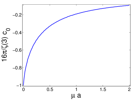
Figure 1: Coefficient $16\pi c_{0}/\zeta(3)$ as a function of $\mu a$.

Regarding the $c_{0}$ coefficient, we find that:

$$c_{0}(\mu a)\;=\;\frac{1}{4\pi}\int_{0}^{\infty}dx\,x\log\Big{[}1-\big{(}\frac{x}{x+\mu a}\big{)}^{2}e^{-2x}\Big{]}\;.$$ (43)

Note that, as shown in Fig. 1, $c_{0}(\mu a)$ interpolates between zero in the limit of large $\mu a$, and $-\zeta(3)/(16\pi)$ for $\mu a\to 0$, the result that corresponds to perfect Neumann boundary conditions (see Eq.(34)).

On the other hand, the $c_{2}$ coefficient can be extracted from the kernel appearing in the second order term for the effective action, $\Gamma^{(2)}$, as follows: In the Taylor expansion around zero-momentum, we denote by $\alpha$ the coefficient of term quadratic in the momentum:

$$f^{(2)}(k_{\parallel})\;=\;f^{(2)}(0)\,+\;\alpha\,k_{\parallel}^{2}\,+\,\ldots$$ (44)

Then, the $c_{2}$ coefficient is given by: $c_{2}(\mu a)\;=\;\frac{a^{2}}{2}\,\alpha\;.$

The contribution to $c_{2}$ coming from $f_{l}$ can be obtained from Eq.(37). Performing the angular integration, it reads

$$c_{2l}(\mu a)=\frac{\mu a}{4\pi}\int_{0}^{\infty}dx\,\frac{x^{3}}{(x+2\mu a)}\frac{1}{(x+2\mu a)^{2}e^{2x}-x^{2}}\,.$$ (45)

The calculation of the other contribution to $c_{2}$, coming from $f_{nl}$, is lengthy but straightforward. We expand the integrand in Eq.(38) in powers of $k_{\parallel}$ keeping just quadratic terms. Performing the angular integration we obtain

$$c_{2nl}(\mu a)=\frac{-1}{4\pi}\int_{0}^{\infty}dx\frac{1}{(2\mu a+x)\left(x^{2}-e^{2x}(2\mu a+x)^{2}\right)^{4}}$$

$$\times x^{3}\left\{e^{2x}x^{4}(2\mu a+x)\left[8(\mu a)^{2}\left(2x^{2}+x-1\right)\right.\right.$$

$$+\left.\left.4\mu ax(4x(x+1)-3)+x^{2}(4x(2x+3)-5)\right]\right.$$

$$+\left.e^{4x}x^{2}(2\mu a+x)\left[32(\mu a)^{4}(x-4)(2x-1)\right.\right.$$

$$+8(\mu a)^{3}x(4x(4x-15)+23)$$

$$+\left.4(\mu a)^{2}x^{2}\left(28x^{2}-94x+29\right)\right.$$

$$+\left.2\mu ax^{3}(8x(3x-8)+19)+x^{4}(4x(2x-3)+7)\right]$$

$$-\left.e^{6x}(2\mu a+x)^{3}\left[-32(\mu a)^{4}-16(\mu a)^{3}x-12(\mu a)^{2}x^{2}\right.\right.$$

$$+\left.\left.12\mu ax^{3}+3x^{4}\right]+x^{7}\right\}.$$ (46)

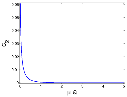
Figure 2: Coefficient $c_{2}$ as a function of $\mu a$.

We have analyzed the behaviour of $c_{2}=c_{2l}+c_{2nl}$ both numerically and analytically. As expected, $c_{2}$ vanishes as $\mu a\to\infty$, which corresponds to the absence of mirrors. The most interesting limit is $\mu a\ll 1$, since this case corresponds to almost-perfect Neumann boundary conditions, a situation where the problems inherent to this case should start to manifest themselves. Indeed: to begin with, one can readily check that the integrand of Eq.(IV) goes like $\sim 1/x$ for $\mu a\sim 0$, signalling the emergence of an infrared divergence, as anticipated in our previous work. Moreover, it can be shown analytically that, when $\mu a\ll 1$,

$$c_{2}(\mu a)\simeq c_{2nl}(\mu a)\simeq-\frac{1}{16\pi}\log(\mu a)\,.$$ (47)

We have also checked this result by computing numerically the logarithmic derivative of $c_{2}$ with respect to $\mu a$, which indeed tends to $-1/(16\pi)$ in the small-$\mu a$ limit. These results are illustrated in Figs. 2 and 3. Fig. 2 depicts $c_{2}$ as a function of $\mu a$, showing that it vanishes for large $\mu a$, while diverges in the opposite limit. As a quantitative check for the small-$\mu a$ behavior given in Eq.(47), in Fig. 3 we show the plot of the logarithmic derivative $\mu a\,dc_{2nl}/d\mu a$.

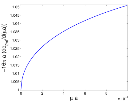
Figure 3: Logarithmic derivative $-16\pi\mu a\,dc_{2nl}/d\mu a$ as a function of $\mu a$.

Collecting the results of this section, we can say that (up to the second order) DE approximation to the Casimir energy reads, for small $\mu a$ (i.e., close to the perfect case):

$$E_{\rm DE}[\psi]\;=\; - \frac{1}{16\pi}\int_{-\infty}^{\infty}dx_{1}\,\frac{1}{\psi(x_{1})^{2}}\left[\zeta(3)\right.$$ (48)

$$+ \left.\log[\mu\psi(x_{1})]\left(\frac{d\psi(x_{1})}{dx_{1}}\right)^{2}\right]\;,$$

and this constitutes one of our main results. The first term is the PFA for the Casimir energy ($E_{\rm PFA})$. The second term contains the first nontrivial correction to PFA ($E_{\rm NTLO}$) for an arbitrary boundary defined by $\psi$. This equation shows that, although the DE is ill defined for Neumann boundary conditions en $2+1$ dimensions, the non-analiticities in the DE appear only in the case of perfect boundary conditions, that is, the parameter $\mu$ acts as an infrared regulator. The physical interpretation anticipated in Ref.ded for the appearance of non-analiticities for Neumann boundary conditions is confirmed by this calculation. Indeed, for $\mu=0$ the field contain massless modes, that are not present for $\mu\neq 0$. Besides, note that the relation between the Casimir energies computed for different values of $\mu$ is encoded in the simple differential equation

$$\mu\frac{dE_{\rm DE}}{d\mu}\;=\;-\frac{1}{16\pi}\int_{-\infty}^{\infty}dx_{1}\,\frac{1}{\psi(x_{1})^{2}}\Big{[}\zeta(3)\,+\,\left(\frac{d\psi(x_{1})}{dx_{1}}\right)^{2}\Big{]}\;,$$ (49)

under the assumption that: $\mu\psi\ll 1$.

V Examples

Let us consider a function $\psi$ describing a parabolic boundary $\psi(x_{1})=a+\frac{1}{2}x_{1}^{2}/R$ facing a straight line, and approximate ($\mu\neq 0$) boundary conditions (EM or Neumann, depending on the field considered).

Note that $a$ plays the role of the minimum distance between the two boundaries, while $R$ is the curvature radius of the parabola at its vertex. From Eq.(48), we obtain the DE approximation to the Casimir energy, expected to be reliable, in this example, when $\epsilon\equiv a/R\ll 1$.

The zeroth-order (PFA) term, calculated from the first line in Eq. (48), reads

$$E_{\rm PFA}=-\frac{\zeta(3)}{16\pi R}\int_{-\infty}^{+\infty}\frac{du}{\left(\epsilon+\frac{u^{2}}{2}\right)^{2}}=-\frac{\zeta(3)}{16\sqrt{2}R}\frac{1}{\epsilon^{\frac{3}{2}}}.$$ (50)

The NTLO correction comes from the second term in Eq.(48). To evaluate the integral, we change the integration variable to $\psi(x_{1})=za$, so that:

$$E_{\rm NTLO} = -\frac{1}{8\pi R}\sqrt{\frac{2}{\epsilon}}\int_{1}^{+\infty}dz\frac{\sqrt{z-1}}{z^{2}}\log\left(\mu R\epsilon z\right)$$ (51)

$$= -\frac{1}{16R}\sqrt{\frac{2}{\epsilon}}\left[1+\log(4\mu R\epsilon)\right].$$

As expected, the NTLO correction to the DE expansion diverges logarithmically in the limit of perfect ($\mu=0$) Neumann boundary conditions, but is finite in the imperfect case.

Besides, we have found it noteworthy that, fixing the value of $\mu$ and taking the limit $\epsilon\to 0$, the ratio between the NTLO and PFA terms becomes independent of $\mu$ and reads

$$\frac{E_{\rm NTLO}}{E_{\rm PFA}}\simeq\frac{2}{\zeta(3)}\epsilon\log\epsilon\,.$$ (52)

This $\epsilon\log\epsilon$ behavior can be contrasted with the case of perfect Dirichlet boundary conditions; in Ref.ded we have shown that, in $2+1$ dimensions,

$$E_{\rm DE}^{(D)}[\psi]\;=\; - \frac{1}{16\pi}\int_{-\infty}^{\infty}dx_{1}\,\frac{1}{\psi(x_{1})^{2}}\left[\zeta(3)\right.$$ (53)

$$+ \left.\frac{[1+6\zeta(3)]}{12}\left(\frac{d\psi(x_{1})}{dx_{1}}\right)^{2}\right]\;,$$

where the upper $(D)$ denotes Dirichlet boundary conditions. Computing explicitly the integrals for the same example, we find

$$\frac{E_{\rm NTLO}^{(D)}}{E_{\rm PFA}^{(D)}}=\frac{\left(1+6\zeta(3)\right)}{24\zeta(3)}\epsilon,$$ (54)

which is linear in $\epsilon$, in contrast with the quasi-perfect Neumann case, that involves a logarithm.

Let us now consider another example, that allows us to make contact with previous results in the literature Bordag2006 : a circle in front a straight line, which is the dimensionally reduced version of the cylinder-plane case. Here, the function $\psi$ defining the curved contour is given by $\psi(x_{1})=a+R\left(1-\sqrt{1-x_{1}^{2}/R^{2}}\right)$, where $R$ is the radius of the cylinder and $a$ is, again, the minimum distance between the circle and the straight line. On physical grounds, we expect the results for either a circle or a parabola in front of a line to be very similar in the $\epsilon\ll 1$ limit. To check this assertion, since the integrals in Eq. (48) cannot be computed analytically for the circle, we have performed a numerical evaluation; in Fig.4 we plot the ratio:

$$\chi=\frac{\frac{E_{\rm NTLO}}{E_{\rm PFA}}}{\frac{2}{\zeta(3)}\epsilon(1+\log[4\mu R\epsilon])},$$ (55)

which compares the ratio between NTLO and PFA terms to the value it should have for the parabolic case, as a function of $\epsilon$. As expected, $\chi\to 1$ for small values of $\epsilon$; exhibiting a similar behavior to the parabola-line case.

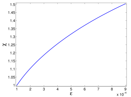
Figure 4: $\chi$ (55) as a function of $\epsilon=a/R$ (circle-line geometry) for $\mu R=0.1$. $\chi$ goes to 1 for small values of $\epsilon$, showing that the NTLO correction in this case is similar to the one of the parabola-line configuration.

Therefore, we conclude that the NTLO correction to PFA is proportional to $\epsilon\log\epsilon$ also for the circle-line geometry, a result that was conjectured for perfect Neumann boundary conditions in Ref.Bordag2006 .

VI Conclusions

In this work, we present results which, we believe, may shed light on some of the properties of the DE approximation to the Casimir energy. In particular, we have studied a phenomenon pointed out in ded , namely, that for perfect Neumann boundary conditions in $2+1$ dimensions, the NTLO correction to the PFA cannot be written as the integral of a local term involving $\psi$ and up to two derivatives of that function. However, as the calculations presented here show explicitly, the NTLO is perfectly well-defined and local when the mirrors are imperfect. In other words, the non-analyticity is an artifact of the idealization of the boundary conditions. And this is corrected by an imperfection, no matter how tiny.

It is worth emphasizing that perhaps a taming of the non analyticity might also be obtained by introducing other, cruder infrared cutoffs, like a mass term for the field. However, as we have shown, it is sufficient to include a rather mild and physically justified modification into the game, which consists of an imperfection in the Neumann conditions, parametrized by a constant that can be tuned to vary the mirrors’ properties.

The same problem can be seen to appear when considering the high temperature limit (for Neumann conditions) in $3+1$ dimensions ded . Mathematically, the integral in momentum space that defines $Z(\psi)$ has an infrared divergence. Based on analogies with results in the context of quantum field theory in non trivial backgrounds, we argued previously that the physical reason for the emergence of nonlocal corrections is the existence of gapless modes, which happens only for Neumann boundary conditions. We have also argued there that, were that the case, for imperfect (and therefore more realistic) boundary conditions, the problem should be cured. We have shown here that this is indeed the case, by providing an explicit example.

We considered the case example of the EM field in $2+1$ dimensions but, in what may be considered a by-product of our study, we have seen that it is dual to a real scalar field, in the understanding that perfect or imperfect conductor boundary conditions for the electromagnetic field correspond, respectively, to perfect of imperfect Neumann boundary conditions for the scalar field.

Regarding explicit results and examples, we have obtained the coefficients of the second order DE, depending on a parameter $\mu$ which measures the departure from perfect boundary conditions, and applied them to evaluate the Casimir energy for the case of a parabola and a circle in front of a line. This enabled us to pinpoint the effect of the would-be infrared dominant contribution to the DE on the resulting energy, for specific geometries. We have also compared the results with those corresponding to Dirichlet boundary conditions, where the problem of non-analyticity of the NTLO correction is not present.

Appendix A Intermediate results on the perturbative expansion for $\Gamma$

We present here some technical details and intermediate results corresponding to the calculation of the effective action to the second order in the function $\eta$. We assume that $\psi(x_{\parallel})=a+\eta(x_{\parallel})$, with $a$ equalling the average of $\psi$.

The term of order $1$ vanishes, and the others can be written in terms of the expanded matrices ${\mathbb{K}}$, of elements $K_{\rm AB}$ (A, B = L, R), which have expressions that we present now. The zeroth order one

$${\mathbb{K}}^{(0)}(x_{\parallel},x^{\prime}_{\parallel}) = {\mathbb{K}}^{(0)}(x_{\parallel}-x^{\prime}_{\parallel})$$ (56)

$$= \int\frac{d^{2}k_{\parallel}}{(2\pi)^{2}}\,e^{ik_{\parallel}\cdot(x_{\parallel}-x^{\prime}_{\parallel})}\;\widetilde{\mathbb{K}}^{(0)}(k_{\parallel})\;,$$

where

$$\widetilde{\mathbb{K}}^{(0)}(k_{\parallel})\;=\;\frac{|k_{\parallel}|+2\mu}{2}\left(\begin{array}[]{cc}1&r(|k_{\parallel}|)e^{-|k_{\parallel}|a}\\ r(|k_{\parallel}|)e^{-|k_{\parallel}|a}&1\end{array}\right)\;,$$ (57)

and $r(x)\;\equiv\;\frac{x}{x+2\mu}$.

Regarding ${\mathbb{K}}^{(1)}$, we see that

$${\mathbb{K}}^{(1)}_{\rm RR}={\mathbb{K}}^{(1)}_{\rm LL}=0\;,$$ (58)

and the off-diagonal elements are given by:

$$K^{(1)}_{\rm LR}(x_{\parallel},x^{\prime}_{\parallel})={\mathbb{K}}^{(1)}_{\rm RL}(x^{\prime}_{\parallel},x_{\parallel})$$

$$=-\frac{1}{2}\int\frac{d^{2}k_{\parallel}}{(2\pi)^{2}}\,e^{ik_{\parallel}\cdot(x_{\parallel}-x^{\prime}_{\parallel})}\,\,e^{-|k_{\parallel}|a}$$

$$\times\left[|k_{\parallel}|^{2}\eta(x_{\parallel})+ik^{\alpha}\partial_{\alpha}\eta(x_{\parallel})\right].$$ (59)

Finally, to the second order, ${\mathbb{K}}^{(2)}_{\rm LL}=0$, and:

$${\mathbb{K}}^{(2)}_{\rm RR}(x_{\parallel},x^{\prime}_{\parallel})=\int\frac{d^{2}k_{\parallel}}{(2\pi)^{2}}\,e^{ik_{\parallel}\cdot(x_{\parallel}-x^{\prime}_{\parallel})}$$

$$\times\left[-\frac{1}{2}\big{(}|k_{\parallel}|^{3}+\frac{k^{\alpha}k^{\beta}}{|k_{\parallel}|}\partial_{\alpha}\partial^{\prime}_{\beta}\big{)}\;\eta(x_{\parallel})\eta(x^{\prime}_{\parallel})\right.$$

$$-\left.i\,|k_{\parallel}|\eta(x_{\parallel})(\partial_{\alpha}\eta(x_{\parallel})+\partial^{\prime}_{\alpha}\eta(x^{\prime}_{\parallel}))\right]\;.$$ (60)

On the other hand, both ${\mathbb{K}}^{(2)}_{\rm LR}$ and ${\mathbb{K}}^{(2)}_{\rm LR}$ are non-vanishing, but it may be seen that they do not contribute to the second order term under the assumption that the average of $\eta$ vanishes.

The Fourier transform of the inverse of ${\mathbb{K}}^{(0)}$ (we need it to calculate the second order term) is given by:

$$\big{(} \widetilde{\mathbb{K}}^{(0)}\big{)}^{-1}(k_{\parallel})=\frac{2}{(|k_{\parallel}|+2\mu)\left(1-r^{2}(|k_{\parallel}|\right)e^{-2|k_{\parallel}|a})}$$ (63)

$$\times \left(\begin{array}[]{cc}1&-r(|k_{\parallel}|)e^{-|k_{\parallel}|a}\\ -r(|k_{\parallel}|)e^{-|k_{\parallel}|a}&1\end{array}\right).$$

The second order term, $\Gamma^{(2)}$ receives two contributions, which we have denoted by $\Gamma^{(2,1)}$ and $\Gamma^{(2,2)}$ in (III). For each one of them we introduce a momentum kernel,

$$\Gamma^{(2,a)}\,=\,\frac{1}{2}\int\frac{d^{2}k_{\parallel}}{(2\pi)^{2}}\,f^{(2,a)}(k_{\parallel})\,|\tilde{\eta}(k_{\parallel})|^{2}\;,\;\;a=1,2\;.$$ (64)

An explicit evaluation of those two kernels yields:

$$f^{(2,1)}(k_{\parallel})\;=\;k_{\parallel}^{2}\;\Big{[}\int\frac{d^{2}p_{\parallel}}{(2\pi)^{2}}\frac{r^{2}(|p_{\parallel}|)}{e^{2a|p_{\parallel}|}-r^{2}(|p_{\parallel}|)}\,\,\frac{\mu}{|p_{\parallel}|+2\mu}\Big{]}$$

$$-\,\int\frac{d^{2}p_{\parallel}}{(2\pi)^{2}}\frac{r^{3}(|p_{\parallel}|)}{e^{2a|p_{\parallel}|}-r^{2}(|p_{\parallel}|)}\,\frac{[p_{\parallel}\cdot(p_{\parallel}+k_{\parallel})]^{2}}{|p_{\parallel}||p_{\parallel}+k_{\parallel}|}\;,$$ (65)

and

$$f^{(2,2)}(k_{\parallel}) = -\int\frac{d^{2}p_{\parallel}}{(2\pi)^{2}}\left\{\frac{r^{2}(|p_{\parallel}|)r^{2}(|p_{\parallel}+k_{\parallel}|)}{\big{(}e^{2a|p_{\parallel}|}-r^{2}(|p_{\parallel}|)\big{)}\big{(}e^{2a|p_{\parallel}+k_{\parallel}|}-r^{2}(|p_{\parallel}+k_{\parallel}|)\big{)}}\right.$$ (66)

$$+ \left.\frac{r(|p_{\parallel}|)r(|p_{\parallel}+k_{\parallel}|)}{\big{(}e^{2a|p_{\parallel}|}-r^{2}(|p_{\parallel}|)\big{)}\big{(}1-r^{2}(|p_{\parallel}+k_{\parallel}|)e^{-2a|p_{\parallel}+k_{\parallel}|}\big{)}}\right\}\frac{[p_{\parallel}\cdot(p_{\parallel}+k_{\parallel})]^{2}}{|p_{\parallel}||p_{\parallel}+k_{\parallel}|}.$$

References

- (1) P. W. Milonni, The Quantum Vacuum, Academic Press, San Diego, 1994; K. A. Milton, River Edge, USA, World Scientific, 2001; M. Bordag, G.L. Klimchitskaya, U. Mohideen, and V. M. Mostepanenko, Advances in the Casimir Effect, Oxford University Press, Oxford, 2009.
- (2) C. D. Fosco, F. C. Lombardo and F. D. Mazzitelli, Phys. Rev. D 84, 105031 (2011).
- (3) G. Bimonte, T. Emig, and M. Kardar, App. Phys. Lett. 100, 074110 (2012); L. P. Teo, M. Bordag, and V. Nikolaev, Phys. Rev. D 84, 125037 (2011); V. A. Golyk, M. Kruger, A. P. McCauley and M. Kardar, EPL 101, 34002 (2013); A. A. Banishev, J. Wagner, T. Emig, R. Zandi and U. Mohideen, Phys. Rev. B 89, 235436 (2014); G. Bimonte, T. Emig and M. Kardar, Phys. Rev. D 90, 081702 (2014); L. P. Teo, Phys. Rev. D 89, 105033 (2014); C. D. Fosco, F. C. Lombardo and F. D. Mazzitelli, Phys. Rev. A 89, 062120 (2014), and references therein.
- (4) B.V. Derjaguin, Koll. Z. 69, 155 (1934); B. V. Derjaguin and I. I. Abrikosova, Sov. Phys. JETP 3, 819 (1957); B. V. Derjaguin, Sci. Am. 203, 47 (1960).
- (5) C. D. Fosco, F. C. Lombardo and F. D. Mazzitelli, Phys. Rev. D 86, 045021 (2012).
- (6) I. Brevik, S. Ellingsen and K. Milton, New J. Phys. 8, 236 (2006). See also Bordag et al in Ref.booksCasimir .
- (7) C. D. Fosco, F. C. Lombardo and F. D. Mazzitelli, Phys. Rev. D 85, 125037 (2012).
- (8) M. Bordag, Phys. Rev. D 73, 125018 (2006).