Ca II Triplet Spectroscopy of Small Magellanic Cloud Red Giants. III. Abundances and Velocities for a Sample of 14 Clusters

Abstract

We obtained spectra of red giants in 15 Small Magellanic Cloud (SMC) clusters in the region of the CaII lines with FORS2 on the Very Large Telescope (VLT). We determined the mean metallicity and radial velocity with mean errors of 0.05 dex and 2.6 km s^-1, respectively, from a mean of 6.5 members per cluster. One cluster (B113) was too young for a reliable metallicity determination and was excluded from the sample. We combined the sample studied here with 15 clusters previously studied by us using the same technique, and with 7 clusters whose metallicities determined by other authors are on a scale similar to ours. This compilation of 36 clusters is the largest SMC cluster sample currently available with accurate and homogeneously determined metallicities. We found a high probability that the metallicity distribution is bimodal, with potential peaks at -1.1 and -0.8 dex. Our data show no strong evidence of a metallicity gradient in the SMC clusters, somewhat at odds with recent evidence from CaT spectra of a large sample of field stars (Dobbie et al., 2014). This may be revealing possible differences in the chemical history of clusters and field stars. Our clusters show a significant dispersion of metallicities, whatever age is considered, which could be reflecting the lack of a unique AMR in this galaxy. None of the chemical evolution models currently available in the literature satisfactorily represents the global chemical enrichment processes of SMC clusters.

1 Introduction

The ages, abundances and kinematics of star clusters are prime indicators of a galaxy’s chemical evolution and star formation history (SFH). This is particularly true for the Small Magellanic Cloud (SMC), which is close enough to provide a wealth of detail in studies including even its oldest stellar populations and also hosts a huge star cluster ensemble. These star clusters also have importance to astronomy beyond the bounds of the SMC. Because of their richness and location in areas of the age-metallicity plane not covered by Milky Way clusters, they have become vital testbeds for theoretical models of stellar evolution at young to intermediate age and low metallicity (e.g., Ferraro et al. 1995; Whitelock et al. 2003). SMC clusters have also been used as empirical templates for interpreting the unresolved spectra and colors of very distant galaxies, including post-starbursts and other pathological cases (e.g., Beasley et al. 2002; Bica & Alloin 1986). The interaction history of the Magellanic Clouds (MCs) with the Galaxy is a matter of current controversy (Kallivayalil et al., 2013), and clusters can serve as important keystones to help pin down the epoch(s) of increased cluster and field star formation due, e.g., to a close galactic encounter.

A major objective is to measure many clusters spanning as wide a range of age, abundance and location as possible in order to maximize our leverage on the chemical evolution as traced by the age-metallicity relation (AMR), metallicity gradient, kinematics and any variation of SFH with location and/or environment. It is also paramount to definitively test for the existence of any bursts of cluster formation (e.g., Rich et al. 2000).

The many free parameters inherent in any realistic chemical evolution model, e.g., that allows radial variations, demands as large a cluster sample as possible. In addition, one requires a homogeneous technique with sufficient precision and accuracy in both age and metallicity. The brightest common stars in clusters older than $\approx$1 Gyr are red giants. Therefore, they are the natural targets for precision measurements of abundances and velocities, especially in extragalactic clusters. The most efficient way to build up a large sample of red giant metallicity and velocity measurements is by using the near-infrared Ca II triplet (CaT) at $\lambda$ $\approx$ 8500 Å, which requires only very moderate resolution spectra as the lines are very strong and very abundance sensitive, and this is near the peak in the flux of red giants. Multi-object spectrographs add an extra dimension of efficiency. Many authors have confirmed the accuracy and repeatability of CaT abundance measurements in combination with broad-band photometry, both optical (Armandroff & Da Costa, 1991) and IR (Mauro et al., 2014), and shown its insensitivity to age (Cole et al., 2004, hereafter C04) and sensitivity to metallicity.

Our group has carried out a number of studies of MC clusters using the powerful CaT technique with FORS2 on the VLT. Our first study (Grocholski et al., 2006, hereafter G06) yielded excellent data for 28 LMC clusters. We found a very tight metallicity distribution (MD) for intermediate-age clusters, no metallicity gradient and confirmed that the clusters rotate with the disk. We followed this up with an initial study of SMC clusters (Parisi et al., 2009, hereafter P09). We obtained spectra for 102 stars associated with 16 SMC clusters. Based on the color-magnitude diagrams (CMDs) from the preimages, spatial distribution, metallicity and velocity analysis, we were able to separate cluster from field stars with very high probability. We determined mean cluster velocities to 2.7 kms^-1 and metallicities to 0.05 dex (random error), from a mean of 6.4 members per cluster. We combined our clusters with those observed by Da Costa & Hatzidimitriou (1998, hereafter DH98), the only previously published CaT study for SMC clusters, and with clusters studied by Kayser et al. (2006), whose study has not been published but whose metallicity values are reported in Glatt et al. (2008b). We found a suggestion of bimodality in the MD and no evidence for a metallicity gradient. The AMR showed good overall agreement with the model of Pagel & Tautvaišienė (1998, hereafter PT98) which assumes a burst of star formation at 4 Gyr, except for two clusters around 10 Gyr which are more metal-rich than the prediction and our 4 youngest clusters, which all lie to lower metallicities than predicted. The simple closed box model of DH98 yields a much poorer fit. The two “anomalous” older clusters are L1 and K3, observed by DH98, who were limited by the technology at the time to single star spectra and could only observe with a 4 m telescope a total of 4 stars per cluster. We also examined the kinematics and found no obvious signs of rotation. Simultaneously, we obtained similar quality radial velocity and metallicity data for $\sim 300$ surrounding field giants. The results for these stars were presented in Parisi et al. (2010, - P10).

However, as shown in P09 and Parisi et al. (2014, hereafter P14), it is clearly necessary to increase the number of SMC star clusters homogeneously studied for a better understanding of the evolution and chemical enrichment processes in this galaxy. Up to this moment, there are only two SMC clusters whose metallicities have been determined from high dispersion spectroscopy and only about 20 with metallicities derived from CaT spectroscopy (P09, DH98). The remaining metal abundance determinations are based on less precise photometric and integrated spectroscopic techniques. Here we present similar excellent CaT data for a new sample of SMC star clusters using the same telescope and instrument as P09 in order to improve our knowledge of the AMR. We also reobserve the problematic clusters L1 and K3 originally observed by DH98 mentioned above in order to help pin down the chemical evolution during this important early phase. This data yields comparable high precision mean metallicity and radial velocity values per cluster as derived in P09. Together, this comprises the first dataset with sufficient precision and accuracy in metallicities and enough clusters to really test chemical evolution models. Secondly, we can better probe previous hints that the metallicity and/or age distributions of SMC clusters exhibit bimodality or similar fine structure, as well as spatial variation in metallicity.

In Section 2 we present our cluster and target selection and in Section 3 the spectroscopic observations are described. Sections 4 and 5 give details about the measurement of radial velocities, equivalent widths and target metallicities, while Section 6 describes the procedure to separate cluster stars from those belonging to the surrounding field. In Section 7 we compare our metallicity determinations with the values found by previous work, in Sections 8 we analyze the metallicity and finally, in Section 9 we summarize our results.

2 Cluster and target selection

In order to increase the number of SMC clusters homogeneously studied by P09, we selected an additional sample of 15 star clusters spread out over a wide region of the SMC. Our clusters are scattered across the main body of the SMC, in environments ranging from the dense central bar to near the tidal radius. In P09 we found a difference between the predictions of the PT98 model and the observations in the 9-10 Gyr age range (L1 and K3, which were observed by DH98) and here we remeasure the abundances of these two clusters to confirm their place in the age-metallicity plane. We also observe a number of old cluster candidates in order to populate this region as much as possible. We have selected all of the richest clusters with ages in the 5 - 10 Gyr range from the work of Rafelski & Zaritsky (2005). There is also a significant discrepancy between the PT98 model and the P09 data for clusters with ages $\sim 1$ Gyr. We are confident that this latter is not the result of significant age effects on the CaT method (C04, Carrera et al. 2008), and therefore also include more $\sim$ 1 Gyr old clusters to investigate the extent of any discrepancies. If confirmed, this would imply a very recent infall of mostly primordial gas into the SMC, which has implications for the chemical evolution of not just the SMC but also potentially the LMC and our Galaxy as well.

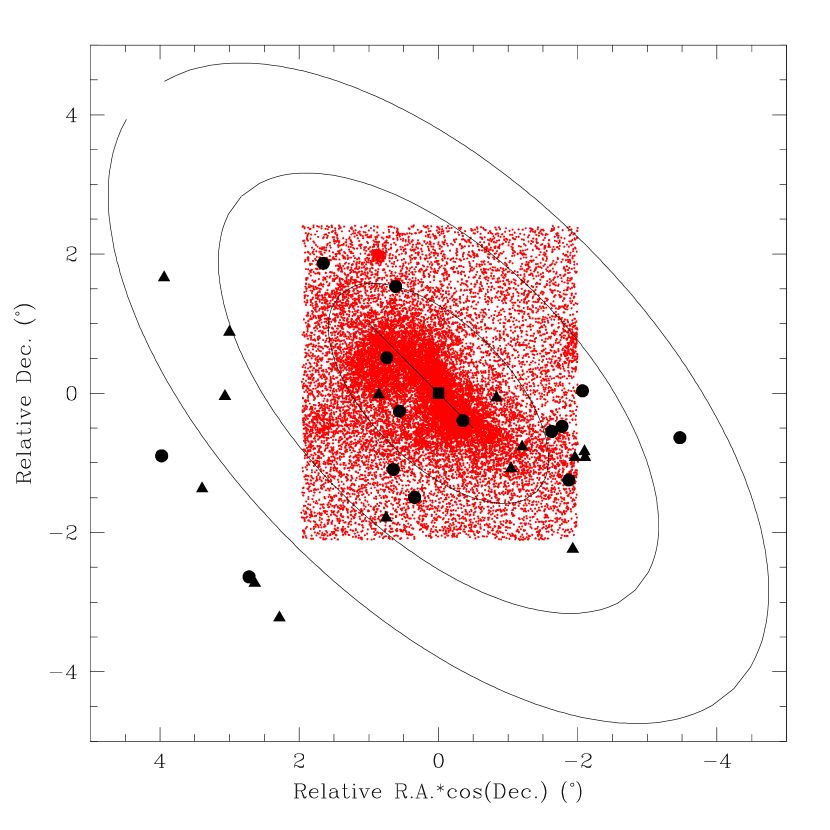
Figure 1: Circles indicate the position of our target clusters in relation to the SMC optical center (square, $\alpha_{J2000}$ = 00^h 52^m 45^s and $\delta_{J2000}$ = 72^∘ 49’ 43”, Crowl et al. 2001) and the SMC bar (line). Triangles represent the position of clusters studied in P09. The ellipses have semi-major axis of 2, 4 and 6 degrees. A SMC map from Zaritsky et al. (2002) has been superposed (Small Magellanic Cloud Photometric Survey for stars with V $<$ 16.)

In Table Ca II Triplet Spectroscopy of Small Magellanic Cloud Red Giants. III. Abundances and Velocities for a Sample of 14 Clusters we present the clusters selected for observation. Included are the identification of these clusters, their equatorial coordinates, the semi-major axis $a$ (Piatti et al., 2007a, b) and the age adopted as well by the respective bibliographic reference. Considering that the reliability of Glatt et al. (2010)’s age determination for cluster K9 and B113 (0.5 and 0.6 Gyr, respectively, the only age values available in the literature) is probably lower than that of the other cluster sample, we adopt the preliminary age (1.09 $\pm$ 0.15 Gyr for K9 and 0.53 $\pm$ 0.07 for B113) derived in our work currently in progress (Parisi et al., 2015). These values were obtained from the $\delta$V parameter measured on the cluster CMD and from the calibration of Carraro & Chiosi (1994), using a procedure similar to the one described in P14. B113 turned out to be too young to reliably apply the CaT technique, so we decided to discard this cluster from our sample. For the sake of consistency with P09, we have adopted the elliptical system introduced by Piatti et al. (2005), in which the corresponding semi-major axis $a$ is used instead of the projected distance to the galaxy center. Although the $a$ values do not consider projection effects, they represent the SMC shape better than a circular system. When selecting the clusters, we covered as large a spatial extension within the SMC as possible so as to examine, among other things, possible metallicity gradients in this galaxy. Figure 1 shows how the selected clusters (circles) are distributed with respect to the SMC bar and center. Clusters studied in P09 (triangles) have also been included in this figure to allow comparison between the two samples.

Spectroscopic targets in each cluster were selected from CMDs built from aperture photometry of preimages in the $V$ and $I$ bands, in the same way as described in detail in P09.

3 Spectroscopic observations

As part of the ESO programs 082.B-0505 and 384.B-0687, spectra of more than $\sim$ 450 stars were obtained in service mode. We used the FORS2 instrument in mask exchange unit (MXU) mode on the Very Large Telescope (VLT), located at Paranal (Chile). Our instrumental setup was identical to that used in G06 and P09, wherein more detailed description can be found, in order to ensure homogeneity.

The spectrum of each star was obtained with exposures of 680 and 635 seconds during the first and second observing runs, respectively. We used slits 1” wide and between 2” and 12” long. The seeing was less than 1” in all cases. Pixels were binned 2x2, resulting in a scale of 0.25”/px. The spectra cover a range of $\sim$ 1500 Å in the region of the CaT ($\sim$ 8500 Å) and have a dispersion of 0.85 Å/px. Most cases have S/N ratio between $\sim$ 20 and $\sim$ 80 pixel^-1, with only a few stars having S/N $\sim$ 15 pixel^-1. Calibration exposures, bias frames and flat-fields were also taken by the VLT staff. We followed the image processing detailed in G06 and P09, using a variety of tasks from the IRAF package.

4 Radial velocity and equivalent width measurements

Our reduction and analysis techniques are identical to those applied in G06 and P09. The program used to measure the equivalent widths (EWs) of the CaT lines uses as input the radial velocity (RV) of the target stars to derive the CaT line centers. These RVs allow us help discriminate probable cluster members from stars belonging to their surrounding stellar fields (see below).

To measure the RVs of our program stars, we performed cross-correlations between their spectra and those of 32 bright template giants observed in Milky Way clusters using the IRAF task fxcor (Tonry & Davis, 1979). This task also transforms observed RVs into heliocentric RVs. We used the template stars of C04 who observed these stars with a setup very similar to ours. The average of each cross-correlation result was adopted as the heliocentric RV of each target. Our heliocentric RVs have a typical standard deviation of $\sim$ 6 km s^-1.

It is well known that errors in centering the image in the spectrograph slit can lead to inaccuracies in determining RVs (e.g., Irwin & Tolstoy 2002). In order to correct this effect, we measured the offset $\Delta x$ between each star’s centroid and the corresponding slit center by inspecting the through-slit image taken immediately before the spectroscopic observation, according to the procedures described by C04 and G06. We calculated the velocity correction $\Delta v$ according to equation (1) from P09. We estimated a measurement precision of 0.14 pixels. Considering our spectral resolution of 30 km s^-1 px^-1, the typical error introduced in the RV, by this effect, turns out to be 4.2 km s^-1. We added this error in quadrature with the one resulting from the cross-correlation. This yields a total of 7.3 km s^-1, which has been adopted as the typical RV uncertainty of an individual star.

To measure EWs, we have used a program whose details can be seen in C04. We adopted the rest wavelength of the CaT lines from Armandroff & Zinn (1988), along with the corresponding continuum bandpasses (see G06’s Table 2). The “pseudo-continuum” for each CaT line was determined by a linear fit to the mean value in each pair of continuum windows. The “pseudo-equivalent width” was calculated by fitting a function to each CaT line with respect to the pseudo-continuum. For spectra with S/N $>$ 20, we fitted to each CaT line a Gaussian $+$ Lorentzian function in order not to underestimate the strength of the wings of the line profile (Rutledge et al. 1997a, b, C04, P09). Then we calculated the metallicity index, $\Sigma W$, defined as the sum of the EWs of the three CaT lines. For spectra with S/N $<$ 20, however, we followed the procedure described in P09, i.e., we fitted only a Gaussian to each CaT line and we then corrected $\Sigma W$ according to equation (2) from P09.

5 Metallicities

The procedure to determine the metallicity of a giant star from CaT lines and the required calibrations are described in detail in G06 and P09. In summary, since our spectra are of high enough quality for all three CaT lines to be well measured, we calculated $\Sigma W$ using the following expression:

$$\Sigma W=EW_{8498}+EW_{8542}+EW_{8662},$$ (1)

in which equal weight was assigned to all three lines. Then, we defined the reduced equivalent width, $W^{\prime}$, to remove the effects of surface gravity and temperature on $\Sigma W$ via its luminosity dependence:

$$W^{\prime}=\Sigma W+\beta(v-v_{HB}).$$ (2)

The difference between the visual magnitude ($v$) of the star and the cluster’s horizontal Branch/red clump ($v_{HB}$) also removes any dependence on cluster distance and interstellar reddening. We measured this magnitude difference using aperture photometry performed on the pre-images, which were uncalibrated, hence the use of lower-case letters to denote the photometry. Finally, the metallicities of the whole cluster sample were derived from the following relationship:

$$[Fe/H]=b+a\times W^{\prime}.$$ (3)

We used the values of $\beta=0.73\pm 0.04$, $b=-2.966\pm 0.032$ and $a=0.362\pm 0.014$, taken from C04, who used an instrumental setup similar to ours to derive them. This is the same calibration used in P09, ensuring our metallicities are homogeneously determined. The C04 calibration is nominally valid in the age range of 2.5 Gyr $\leq$ age $\leq$ 13 Gyr and in the metallicity range -2.0 $\leq$ [Fe/H] $\leq$ -0.2.

Following this procedure, we derived individual metallicities of the observed red giant stars with errors ranging from 0.09 to 0.32 dex, with a mean of 0.16 dex.

6 Cluster membership

To discriminate cluster members from non-member stars belonging to the surrounding field as much as possible, we followed the procedure described in G06 and P09. Using the coordinates from the aperture photometry, we determined the center of each cluster by building projected histograms in the $x$ and $y$ directions. We then fitted Gaussians to these histograms (using the gnuplot program) and adopted the center of these Gaussians as the cluster center. We then obtained the cluster radial profile based on star counts carried out over the entire area around each cluster.

As an example to illustrate the process employed for all clusters, we show in Figure 2 the radial profile obtained for cluster K 3. The vertical line on the profile represents the adopted cluster radius, which will be used in the subsequent analysis to evaluate cluster membership. Note that the adopted cluster radius can differ from the more typical definition, in which the radius is the distance from the center to the point where the stellar density profile reaches that of the background (Piatti et al., 2007c). In our analysis, we adopted in most cases smaller radii than those resulting from this definition in order to maximize the probability of cluster membership.

Once the cluster radii were determined, we built instrumental CMDs for each cluster using aperture photometry derived from our $v–$ and $i-$band pre-images. These CMDs were constructed using only the stars located within the apparent radius. Then, we measured $v_{HB}$ as the median value of all stars inside of a box that is 0.7 mag in $v$ and 0.3 mag in $v-i$ and centered on the red clump (RC) by eye. We preferred to use the median value instead of the mean value for the reasons stated in P09. Errors in $v_{HB}$ are taken as the standard errors of the median.

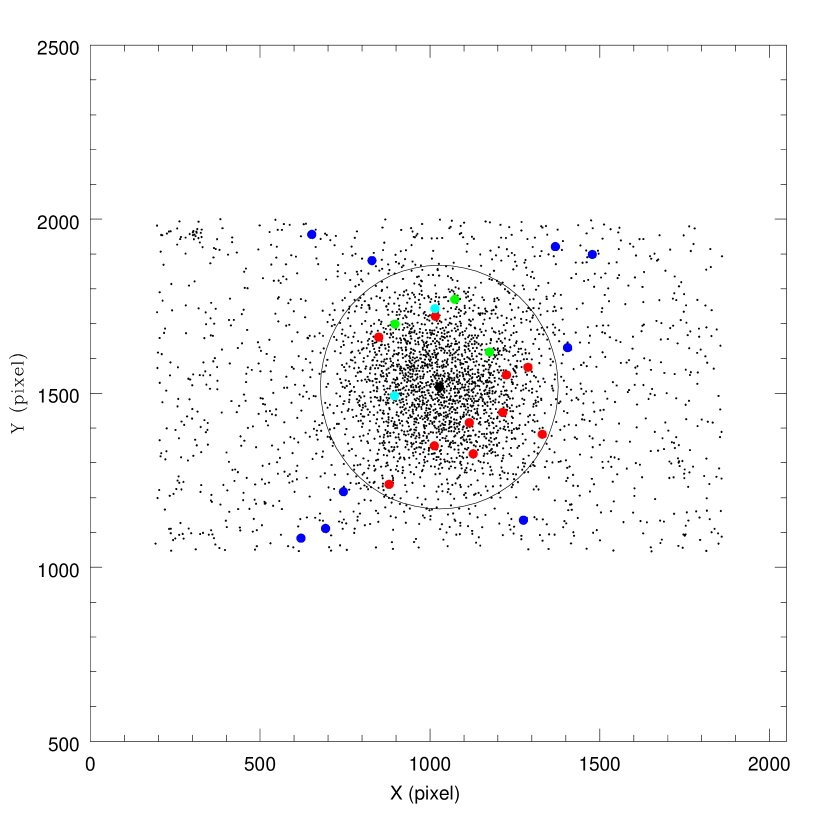
Figure 3: Schematic finding chart of cluster K 3. Our spectroscopic target stars are represented by the large filled circles and the adopted cluster radius is represented by a large circle. Blue circles indicate non-members outside the cluster radius. Teal and green circles represent non-members eliminated due to discrepant RV or metallicity, respectively. Red circles indicate final cluster members.

As the first step to evaluate cluster membership, we considered as non-members those stars located outside the adopted cluster radius. As an example, we plot in Figure 3 the $xy$ positions of all stars photometrically observed in and around K 3. Our spectroscopic targets are represented by the large filled symbols, and the adopted cluster radius is indicated by the large circle. The target stars in blue are considered non-members due to their location outside the adopted cluster radius.

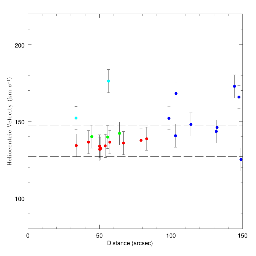
Figure 4: Radial velocity vs. distance from the cluster center for K 3 targets. Horizontal lines represent our velocity error cut and the vertical line the adopted cluster radius. Color code is the same as in Figure 3.

The second and third steps to discriminate cluster members from non-members was to analyze the behavior of the RVs and metallicities as a function of distance from the cluster center. Figure 4 shows how the RVs of the observed stars in K 3 vary as a function of clustercentric distance. We have adopted an intrinsic cluster velocity dispersion of 5 km s^-1 (Pryor & Meylan, 1993), which added in quadrature with our adopted RV error (7.3 km s^-1), yields an expected dispersion of $\sim$ 9 km s^-1. We have rounded this up and adopted 10 km s^-1 in our analysis. Horizontal lines in Figure 4 show our cuts in RV = $\pm$ 10 km s^-1, which represents the expected RV dispersion within the cluster. These RV cuts were adopted taking into account the fact that the members of a cluster should have a velocity dispersion lower than that of the field stars. The vertical line in Figure 4 again shows the adopted cluster radius.

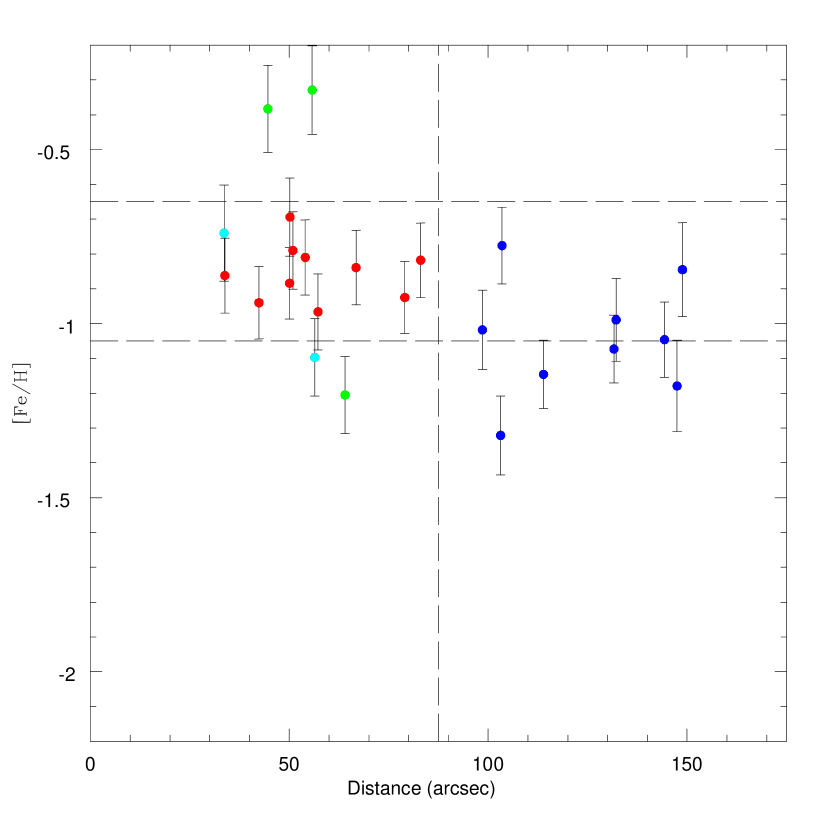
Figure 5: Metallicity vs. distance from the cluster center for K 3 targets. Horizontal lines represent the [Fe/H] error cut and the vertical line the adopted cluster radius. Color code is the same as in Figure 3.

Figure 5 shows how the metallicities of the observed stars vary as a function of the distance from the center of K 3. Since we have estimated a typical metallicity error of 0.16 dex for an individual star, we adopted an [Fe/H] error cut of $\pm$ 0.20 dex, represented by horizontal lines in Figure 5. As in Figure 4, the vertical line in Figure 5 represents the cluster radius. Following the G06 and P09 color code, we have adopted in Figures 4 and 5 blue symbols to represent non-members lying outside the cluster radius, teal and green symbols for non-members we eliminated for having RV and metallicity discrepancy, respectively, and red symbols for stars that have passed all three cuts and are therefore considered cluster members. This procedure has been followed for each cluster in our sample. Figure 6 shows $\Sigma W$ vs. $v-v_{HB}$ for our cluster sample.

Table 2 also shows the identification of the star, heliocentric RV and its error in columns (1), (2) and (3), $v-v_{HB}$ in column (4), $\Sigma W$ and its error in columns (5) and (6) and metallicity and its error in columns (7) and (8).

Finally, using these member stars, we calculated the mean cluster RV and the mean cluster metallicity and their standard error of the mean. The final results are presented in Table 3 where we successively list: cluster ID, the number $n$ of stars considered to be members, the mean heliocentric RV with its error and the mean metallicity followed by its error. Errors in RV and metallicity correspond to the standard error of the mean.

7 Comparison to previous metallicity determinations

Before analyzing our metallicity results, it is important to see how they compare with any previous determinations by other authors. The current CaT metallicities for B 99, H 88-97, K 8, K 9 and OGLE 133 appear to be the first metallicity determinations made for these clusters. Only three (K 3, L 1 and L 113) out of the remaining nine clusters of our sample have spectroscopic metallicities determined by DH98 from CaT, whereas the metallicity for HW 40, K 3, K 6 and L 113 has been estimated from integrated spectroscopy (Piatti et al., 2005; Dias et al., 2010, 2014). Other metallicity determinations reported in the literature, for the previously studied clusters, are based on photometric techniques, mostly on the Washington photometric system (Piatti, 2011a; Piatti et al., 2011b; Piatti, 2011c; Mighell et al., 1998; Piatti et al., 2001, 2007b).

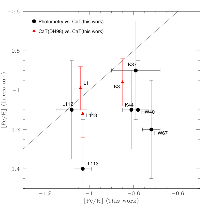
Figure 7: Comparison of our spectroscopic mean cluster metallicities and those derived by other authors from Washington photometry (filled circles) and by DH98 from CaT (triangles). The line shows one-to-one correspondence.

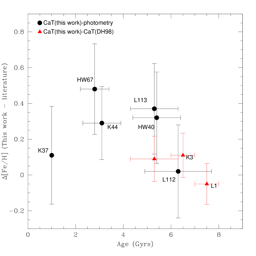
Figure 8: Difference between our CaT metallicities and those derived by other authors as a function of age. Symbols are the same as in Figure 7.

In Figure 7, we have plotted the metallicities available in the literature as a function of those derived from our present work for the clusters in common. The solid line indicates one-to-one correspondence. In addition, Figure 8 shows the difference between both metallicity values as a function of cluster age. In Figures 7 and 8, filled circles stand for clusters whose metallicities haven been previously determined by other authors from Washington photometry. Triangles represent the three clusters for which DH98 derived CaT metallicities. Our CaT metallicities are in excellent agreement with those found by DH98, with the difference between them generally smaller than 0.1 dex, certainly within the respective errors, and with no systematic offset. This gives us added confidence that our metallicities are on solid footing. On the other hand, the mean difference (in absolute value) between our metallicities and those derived from Washington photometry is 0.26 $\pm$ 0.17 dex, with our values being more metal-rich. In P09, we also compared our CaT-based metallicities with those based on Washington photometry for 11 clusters and found no systematic difference. Here all 6 Washington metallicities are lower than our values. However, the differences are not very significant given the much larger photometric metallicity error bars. Because of the age-metallicity degeneracy, a significant variation of metallicity can affect cluster ages when they are determined by theoretical isochrones, which may, in turn, affect the conclusions drawn about the AMR. We plan to determine the ages of the clusters studied in this paper following the same procedures as in P14, in a subsequent paper.

Regarding metallicity determinations from integrated spectroscopy, we find a reasonable agreement with our values for clusters HW 40 and K 6. However, this agreement is substantially poorer for clusters L 113 and K 3. There are several previous metallicity determinations from integrated spectroscopy for these two clusters. From those determinations, the reported values of [Fe/H] are -1.2, -1.8 (Piatti et al., 2005; Dias et al., 2010) for K 3 and -1.4, -2.6 (Dias et al., 2010) for L 113. The minimum difference between both spectroscopic metallicity determinations (integrated and CaT) is 0.35 dex; it is much larger, however, if the most metal-poor values in the literature are adopted. For the integrated spectra technique, it is harder to assess the significance of the offset with our values given the lack of errors for some of the clusters. We note that the CaT technique is generally believed to be more robust, less sensitive to age and observing technique and model-independent and so should be given higher weight.

Figure 8 shows there is no significant trend for the offset in metallicity with cluster age.

8 Metallicity analysis

In order to best analyze the SMC chemical properties, it is optimal not only to have available a cluster sample larger than the one we investigate here but also to maintain homogeneity as much as possible. For this reason, we added to the present sample other clusters having well-determined metallicities on a scale judged to be the same as, or similar to, our’s. As mentioned, in P09 the metallicity of 15 SMC clusters was determined following exactly the same procedure as in this study. It is therefore appropriate to add them to the present sample. The ages we adopt for these 15 clusters are those determined by P14 from the $\delta V$ parameter using the Carraro & Chiosi (1994) calibration. In addition, our sample has been complemented by the L 11, NGC 121 and NGC 339 metallicities from DH98 and ages based on deep HST data (Glatt et al., 2008a, b). The corresponding metallicity (converted to the scale of Carretta & Gratton 1997) and age values reported by Glatt et al. (2008b) for NGC 416, L 38 and NGC 419 were also included. In both studies, metallicities have been inferred from the CaT technique. Thus, we have a sample consisting of 35 clusters homogeneously studied with accurately determined metallicities. It is important to remark that this is at present the largest SMC cluster sample with well-determined metallicities on a homogeneous scale. As part of our sample, we also included NGC 330, whose metallicity was obtained from high dispersion spectroscopy (-0.94 $\pm$ 0.02, Gonzalez & Wallerstein 1999). We note that Hill (1999) also studied NGC 330 with high dispersion spectroscopy, finding a slightly higher value (-0.82 $\pm$ 0.11 dex). Both values are in agreement within the errors but the Gonzalez & Wallerstein (1999) is more precise so we adopt their value, as well as for consistency with our previous works (P09, P14).

8.1 Metallicity distribution

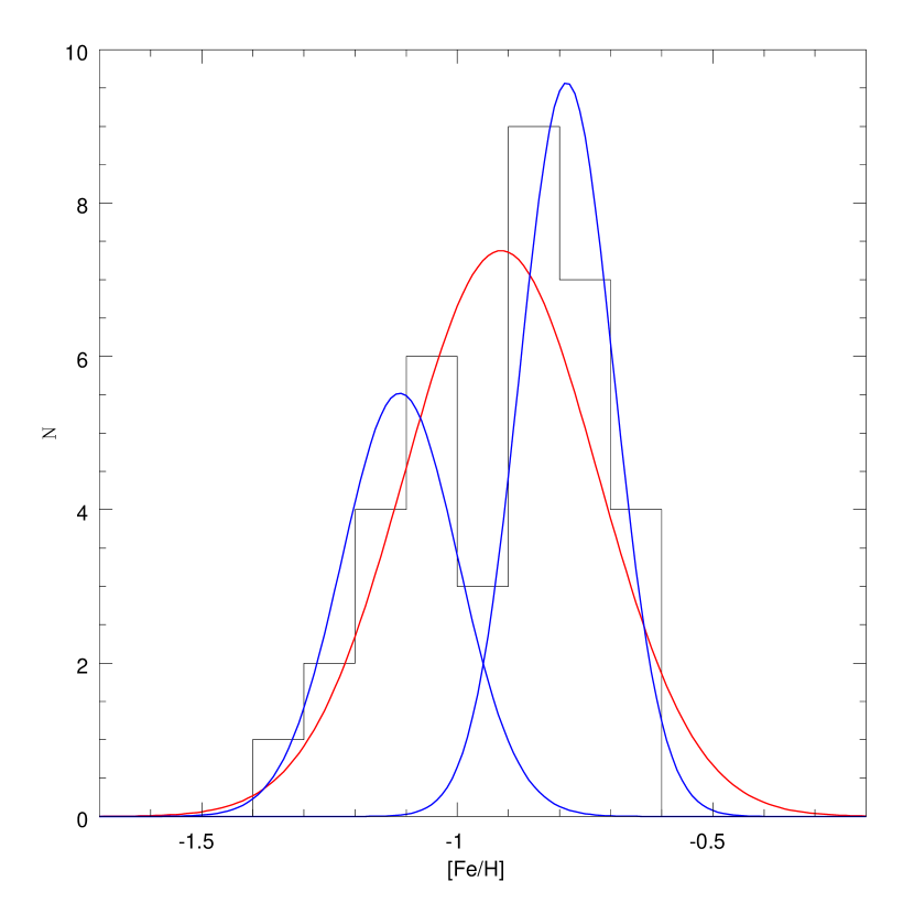
Figure 9: Metallicity distribution of SMC clusters: 14 from the present work, 15 from P09, 3 from DH98, 3 from Glatt et al. (2008b) and NGC 330 (Gonzalez & Wallerstein, 1999). Red and blue lines represent the unimodal and bimodal fits, respectively, according to the GMM algorithm independent of the bin selected for plotting this histogram.

Figure 9 shows the MD of the 36 SMC clusters. It can be seen that this distribution suggests the existence of bimodality with possible peaks at about [Fe/H] = -1.1 and -0.8, respectively. For a more quantitative analysis of the possible existence of bimodality, we applied the GMM (Gaussian Mixture Model, Muratov & Gnedin 2010). The unimodal fit (red line in Figure 9) gives $\mu$ = -0.914 and $\sigma$ = 0.189, while the fit of two Gaussians (heteroscedastic split, blue lines in Figure 9) gives $\mu_{1}$ = -1.112, $\mu_{2}$ = -0.786, $\sigma_{1}$ = 0.114 and $\sigma_{2}$ = 0.092. In the homoscedastic case ($\sigma_{1}$ = $\sigma_{2}$), we found $\mu_{1}$ = -1.125, $\mu_{2}$ = -0.793 and $\sigma$ = 0.102. We obtained p values of 0.042 and 0.16 for the homoscedastic and heteroscedastic fits, respectively. This means that there is a probability of 4.2% (homoscedastic case) and 16% (heteroscedastic case) probability of being wrong in rejecting unimodality. These values are in agreement with the probability given by the parametric bootstrap of 86% that the distribution is indeed bimodal. The GMM algorithm calculated the separation of the peaks, finding D = 3.36 $\pm$ 0.73 and a kurtosis value of -0.852. To accept a bimodal distribution, values of D $>$ 2 (Ashman et al., 1994) and kurtosis $<$ 0 are required. The values derived for D and kurtosis support, therefore, the probability of bimodality. It should be made clear that these results do not depend on the metallicity bin, since the GMM is not applied to the histogram (e.g., the one shown in Figure 9 ) but to the metallicity values. In P09 we had already found a suggestion of bimodality in the cluster MD, but now the evidence is substantially stronger. Mucciarelli (2014) published results based on a high resolution spectroscopic survey of  200 SMC red giant field stars performed with FLAMES (VLT). He found a main peak at $\sim$ -0.9/-1.0 dex, with a secondary peak at [Fe/H] $\sim$ -0.6, and suggested bimodality was present. Note that his peaks are offset from ours by about 0.2 dex. Also, we find more objects in the metal-rich peak instead of the metal-poor peak, although the difference is much less dramatic than found by Mucciarelli (2014). However, recently Dobbie et al. (2014) did not find evidence of any secondary peak in a considerably larger field sample (more than 3000 stars), in agreement with our field sample (P10; Parisi et al. in preparation). Obviously, more clusters studied with reliable metallicities are needed to definitively investigate the bimodality of the SMC cluster MD.

8.2 Metallicity gradient

Another important aspect to examine is the possible existence of a metallicity gradient in the SMC. The existence or not of a gradient can be crucial for understanding the stellar formation and evolution processes in this galaxy. Important efforts to confirm or deny the existence of a metallicity gradient in the SMC have been made recently (e.g., Piatti et al. 2007a, b; Carrera et al. 2008; Cioni 2009; P09; P10). Despite their efforts, these authors have not come to an agreement about the nature of any metallicity gradient. Quite recently, however, Dobbie et al. (2014) found a clear -0.075 $\pm$ 0.011 dex deg^-1 gradient, based on the spectroscopic CaT metallicities of about 3000 SMC red field giants. They found this change of metallicity with radius within 4^∘ of the center, with no significant change beyond this. Previously, based on a smaller sample but also from CaT metallicities of field red giants, Carrera et al. (2008) found hints of a radial metallicity gradient.

In this study, we analize the possible existence of an SMC metallicity gradient using our sample of 36 star clusters. As in P09, our sample has been divided in two groups: (i) those clusters located at a distance from the SMC center less than 4^∘ and (ii) those located beyond this value. This division was based on the suggestion of Piatti et al. (2007a, b) which sustains that the inner cluster mean metallicity ($a$ $<$ 4^∘) is larger than the mean metallicity of the clusters located in the outer region ($a$ $>$ 4^∘). A total of 25 clusters in our sample lie in the SMC inner region (within 4^∘), while 11 of them lie in the outer region. The mean metallicities (and their respective standard deviations) are -0.88 (0.18) and -1.00 (0.19) for the SMC inner and outer regions, respectively. The associated standard error of the mean are 0.04 and 0.06 dex for inner and outer clusters, respectively, which implies a statistical significance of $\sim$ 1.7 sigma between the two mean values.

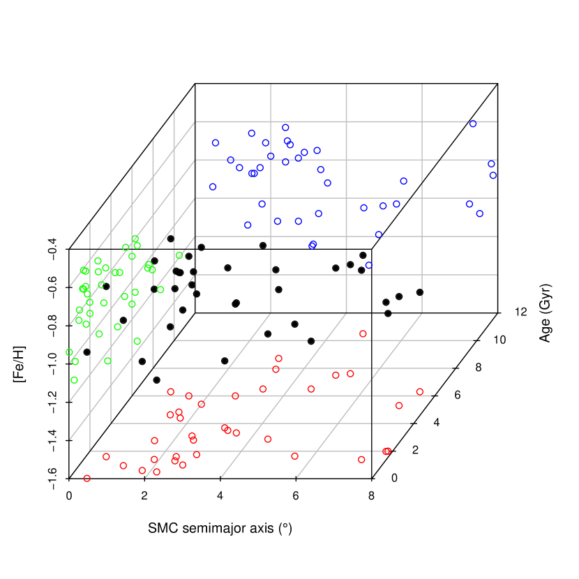
Figure 10: A 3D plot using the quantities [Fe/H], age and semi-major axis $a$ for our 36 cluster sample. The projection on each plane is represented in different colors.

Figure 10 shows a three-dimensional representation of our cluster sample, the dimensions being metallicity ([Fe/H]), age and semi-major axis $a$. The age-metallicity relation (AMR) will be analized in the next section. Here, we focus on the projections on the (age,$a$) and ([Fe/H],$a$) planes. If only these two projections were considered, there seems to be a general trend of the metallicity to decrease with distance from the galaxy center $-$ at least within the first 4^∘ from the galaxy center $-$ and of the age to increase with distance. However, it is worth considering that both the age and metallicity dispersions are remarkably large. Note the curious V-shape presented by the metallicity distribution in the ([Fe/H],$a$) diagram with the vertex around 4-5^∘, which is also visible in Piatti (2011c).

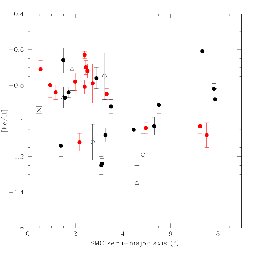
Figure 11: Cluster [Fe/H] as a function of semi-major axis $a$ for the sample of 36 SMC clusters described in Figure 9. Red and black circles represent clusters from the present work and P09, respectively. Clusters from DH98 are shown by open circles while triangles are clusters from Glatt et al. (2008b). NGC 330 is represented by a cross.

The behavior of the metallicity as a function of the semi-major axis $a$ for the 36 star clusters of our sample can be observed in Figure 11. The meaning of the different symbols is explained in the figure caption. Although this figure suggests the possibility that the metallicity decreases with the semi-major axis $a$ (at least within the first 4-5^∘ from the galaxy center), in agreement with Dobbie et al. (2014) findings, it is difficult to assert that there is a metallicity gradient in our cluster sample. This is mainly due to the large metallicity dispersion for each $a$ value, which may be as large as 0.5 dex. The weighted and unweighted linear fits of the data within 4^∘ give slope values of -0.04 $\pm$ 0.04 and -0.05 $\pm$ 0.04, respectively. Both the slopes and their errors have comparable values; thus the fits are not statistically significant, although the formal value we find (-0.05 $\pm$ 0.04) is in reasonable agreement with that of Dobbie et al. (2014) (-0.075 $\pm$ 0.011). As for ages, it is necessary to remember that the cluster ages here analyzed are on a less homogeneous scale than the metallicities. Dobbie et al. (2014) interpreted the metallicity gradient due to a larger fraction of young stars toward the center of the galaxy, in concordance with other authors in previous works (e.g., Carrera et al. 2008; Weisz et al. 2013; Cignoni et al. 2013). Considering the ages of our 36 star clusters, the ratio of clusters younger than 4 Gyr to older changes from 1.5 inside 4^∘ to 0.83 outside. These numbers are in agreement with Dobbie et al. (2014)’s idea but it is hard to assess the statistical significance given the small sample. Also in P14 we find no age gradient from a sample of 50 star clusters with ages determined in a similar scale. Therefore, although we believe there is a suggestion of a metallicity gradient in our cluster sample, at least within the innermost 4-5^∘, we cannot confirm it. Beyond that, any potential gradient becomes very flat or in fact turns around and rises. Note that indeed this is the case in the Galaxy, where the disk metallicity gradient flattens out beyond about 10-12 kpc (e.g., Twarog et al. 1997). It is worth mentioning that a sample of $\sim$ 750 red field giants (P10; Parisi et al. in preparation) shows a metallicity gradient in the inner 4^∘ in reasonable agreement with that of Dobbie et al. (2014), with the metallicity dispersion of field stars much lower than that of the clusters. Dobbie et al. (2014) found that the SMC fields studied in P10 clearly exhibit a metallicity gradient, at least within the first 4^∘ from the galaxy center. The problem arises when clusters are studied alone or combined with field stars, in which case the large metallicity dispersion of the clusters blurs the gradient.

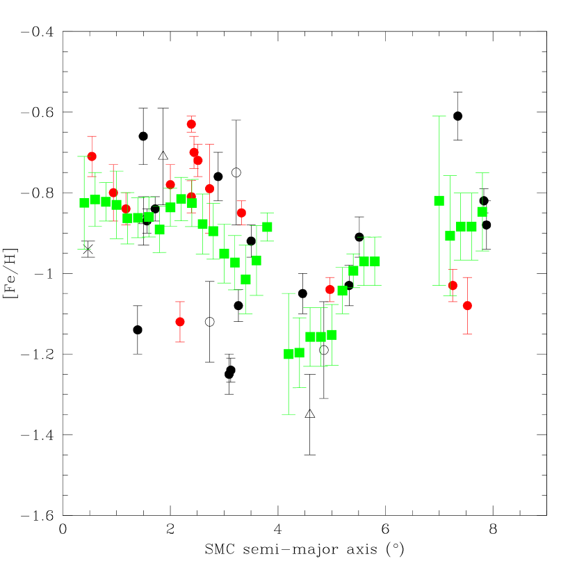
Figure 12: Mean metallicity vs. mean semi-major axis $a$ (green squares). Error bars correspond to the standard error of the mean. The other symbols are the same as in Figure 11.

To further investigate the above mentioned V-shape in the ([Fe/H],$a$) diagram, we divided the $a$ parameter in steps of 0.2^∘. We then chose those clusters within $\pm$0.5^∘ in each bin and calculated the mean metallicity and the error of the mean (green squares in Figure 12). The remaining symbols in Figure 12 have the same meaning as in Figure 11. We note that from 0^∘ to 2.5^∘, the trend of the metallicity appears to be flat. Then, the mean metallicity decreases exhibiting a minimum at $\sim$ 4-5^∘. Finally, the mean metallicity rises to become flat again in the outermost parts. If this behavior is real, it is indeed curious and difficult to explain, especially if the large metallicity dispersion is taken into account.

8.3 Age-Metallicity relation

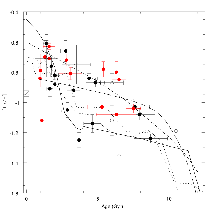
Figure 13: Age-Metallicity Relation for the full sample (see caption of Figure 11 for details about symbols). Observations are compared with different models: DH98 (short dashed line), PT98 (solid line), Carrera (2005, long dashed line) and Cignoni et al. (2013, dotted lines).

Figure 13 shows the relation between age and metallicity for the 36 clusters of our sample. Symbols in this figure hold the same meaning as in Figure 11. In an attempt to understand how the SMC chemical evolution occurred, the observational data were compared with different models currently available in the literature. The solid line in Figure 13 represents the PT98 bursting model, which posits star formation bursts. Such an initial burst could have been followed by a long period with no chemical enrichment whatsoever between 11 and 4 Gyr ago, while a more recent star formation burst could have considerably increased metallicity in the SMC. The short dashed line corresponds to the simple closed box model (DH98), which assumes that the SMC chemical enrichment took place continuously and gradually throughout the galaxy’s lifetime. The long dashed line represents the best fit found by Carrera (2005) for a large field star sample studied using the CaT technique. Finally, the dotted lines are the age-metallicity relations (AMRs) obtained by Cignoni et al. (2013) from the study of six SMC fields.

In general terms, it is observed that for each age interval there exists a metallicity dispersion of $\sim$ 0.5 dex, which is very significantly larger than the corresponding metallicity determination errors. Clusters do not appear to favor any of the models currently available. This seems to suggest that there is not a unique cluster AMR in the SMC. Either the galaxy was not well mixed chemically initially and/or the chemical evolution was not a simple, smooth, global process, with the clusters being more affected by dispersion processes than their offspring, the field stars.

Taking these findings into account, it would be interesting to analyze the behavior of cluster metallicities in relation to their ages in different regions of the SMC. Our cluster sample is still statistically too small to examine the AMR in particular regions of the SMC. However, a first approach to this study can be carried out by examining the AMR at different distances from the SMC center. Our sample was divided in four groups according to semi-major axis $a$, namely: 0${}^{\circ}-$ 2^∘, 2${}^{\circ}-$ 4^∘, 4${}^{\circ}-$ 6^∘ and 6${}^{\circ}-$ 8^∘. The resulting AMR for each of these four groups can be observed in Figure 14. The corresponding $a$ intervals are shown in each panel. The figure includes the same models as Figure 13. Note that clusters situated at distances from the SMC center larger than 4^∘ seem to reasonably follow the bursting model. The same does not occur with the inner clusters that better fit the tendencies of DH98 and Carrera (2005) models. We point out, however, that in the outermost two $a$ intervals, the number of clusters is not significant enough to achieve conclusive results. On the other hand, there are at least 6 clusters in the first two $a$ intervals considerably more metal-poor than predicted by Carrera (2005) and DH98 models. It is then absolutely necessary to have a larger cluster sample available so as to examine any possible AMR variations in greater detail.

Several years ago, Tsujimoto & Bekki (2009) computed two models of chemical evolution considering the merger of two galaxies with different mass ratios (1:1 and 1:4). They also computed a model with no merger. They compared these models with the AMR of cluster and field stars taken from the literature, derived from photometric (Piatti et al., 2001, 2005, 2007b, 2007c; Glatt et al., 2008a, b) and spectroscopic (Da Costa & Hatzidimitriou, 1998; Kayser et al., 2006; Carrera et al., 2008) studied. They suggested that a major merger occurred in the SMC $\sim$ 7.5 Gyr ago, evidenced by a dip in the AMR around that time. The cluster sample used by Tsujimoto & Bekki (2009) is very heterogeneous in both age and metallicity. Also, the photometric metallicities are considerabley less precise that the spectroscopic ones (P09). With this in mind, it is of interest to compare the three models from Tsujimoto & Bekki (2009) with the sample here studied, which is homogeneous, especially in metallicity values. Figure 15 shows our AMR in two intervals of $a$ (0${}^{\circ}-$ 4^∘ and 4${}^{\circ}-$ 8^∘). Solid and dashed lines represent models of mergers having a mass ratio of 1:4 and 1:1 respectively, while the dotted line represents the model without a merger.

It can be seen in Figure 15 that when distances from the galaxy center are smaller than 4^∘, our observations do not seem to favor any of the scenarios proposed by Tsujimoto & Bekki (2009). The large metallicity dispersion is the salient feature. In this $a$ interval, the metallicity dip proposed by Tsujimoto & Bekki (2009) is not as clearly as in these authors’ work. Conversely, our observations distinctly tend to favor merger scenarios in those clusters located beyond 4^∘. The two models that assume mergers reproduce the clusters within this interval fairly well. There is, however, an exception: the cluster located at ($\sim$ 1.5 Gyr, $\sim$ -0.6 dex). Our evidence thus suggests the possibility that the SMC had suffered a merger event affecting mainly the outer part of the galaxy, which would be a possible explanation for the differences found between the SMC outer and inner regions, mainly with regard to the metallicity gradient and AMR.

9 Summary

We used the FORS2 instrument on VLT to obtain spectra in the region of the CaT lines of more than $\sim$ 450 red giant stars belonging to 15 clusters in the SMC and their surrounding fields. Following exactly the same procedure as in P09, we determined their metallicities and RVs with typical errors of 0.16 dex and 7.3 km s^-1 per star, respectively, after discarding one cluster too young for the metallicity calibration. We analyzed cluster membership using as criteria distance from the cluster center, RV, and metallicity (G06, P09). From those stars considered to be cluster members, we derived the mean metallicity and RV of the 14 remaining clusters. We obtained mean cluster velocities and metallicities with mean errors of 2.6 km s^-1 and 0.05 dex, from a mean of 6.5 members per cluster. Ages of our 14 clusters were adopted from the literature.

Using this information, together with that for other clusters similarly studied, we analyze the chemical properties of the SMC cluster system. Specifically, we added to our present sample 15 clusters whose metallicities and ages were derived in P09 and P14, respectively, and also included 7 other clusters previously studied by DH98, Glatt et al. (2008a, b) and Gonzalez & Wallerstein (1999). The metallicities of these additional clusters have been determined from CaT except one, NGC 330, whose metallicity was inferred from high dispersion spectroscopy. Consequently, we compiled a sample of 36 SMC clusters with accurate metallicities. So far this is the largest SMC cluster sample with accurate and homogeneous metallicities.

Our main results are the following:

• The MD of our cluster sample appears to be bimodal, with potential peaks at $\sim$ -1.1 and -0.8 dex. We applied the Gaussian Mixture Model (Muratov & Gnedin, 2010), obtaining a high probability that our data can be represented by two as opposed to a single Gaussian function.

• Our data show a tendency of metallicity to decrease with distance from the center of the galaxy, at least out to about 5^∘, where any potential gradient appears to flatten or even turn around, but we can not confirm the existence of a metallicity gradient in our cluster sample, mainly because of the large metallicity dispersion.

• We corroborate the P09 finding, now with a larger sample of clusters, that the AMR presents a significant metallicity dispersion of about 0.5 dex, a value that exceeds the errors associated with the determination of the metallicity. This dispersion of metallicities may be evidence that there is not a single AMR in the SMC. In fact, none of the chemical evolution models currently available in the literature turn out to be a good representation of the general trend of [Fe/H] with age. A larger statistical cluster sample is needed to analyze the AMR in different regions of the SMC.

Table 1: SMC Clusters sample

Cluster	RA (J2000.0)	Dec (J2000.0)	$a$	Age	Age
	($h$ $m$ $s$)	(∘ ′ ′′)	(∘)	(Gyr)	reference
B 99, OGLE-CL SMC 122	01 00 30.52	-73 05 14.40	1.174	0.95	1
B 113	01 02 55.75	-73 20 18.60	1.770	0.53	2
H 86-97, OGLE-CL SMC 43	00 47 53.42	-73 13 14.10	0.540	1.60	1
HW 40	01 00 25.11	-71 17 43.80	2.000	5.40	3
HW 67	01 13 01.82	-70 57 47.10	2.513	2.80	4
K 3, L 8, ESO 28-19	00 24 47.70	-72 47 00.01	3.322	6.50	5
K 6, L 9, ESO 28-20	00 25 26.60	-74 04 29.70	2.390	1.60	6
K 8, L 12	00 28 02.14	-73 18 13.60	2.440	1.30	1
K 9, L 13	00 30 00.26	-73 22 40.70	2.180	0.50	2
K 37, L 58	00 57 48.53	-74 19 31.60	2.730	1.00	1
K 44, L 68	01 02 06.34	-73 55 22.70	2.391	3.10	7
L 1, ESO 28-8	00 03 54.00	-73 28 18.00	4.968	7.50	5
L 112	01 36 01.00	-75 27 00.30	7.524	6.30	8
L 113, ESO 30-4	01 49 30.00	-73 43 40.00	7.252	5.30	9
OGLE-CL SMC 133	01 02 31.86	-72 19 05.30	0.941	6.30	1

.

References. — (1) Rafelski & Zaritsky (2005), (2) Parisi et al. (2015), (3) Piatti (2011a), (4) Piatti (2011c), (5) Glatt et al. (2008b), (6) Piatti et al. (2005), (7) Piatti et al. (2001), (8) Piatti et al. (2011b), (9) Piatti et al. (2007b)

Table 2: Measured values for member stars

ID	RV	$\sigma_{RV}$	$v-v_{HB}$	$\Sigma W$	$\sigma_{\Sigma W}$	[Fe/H]	$\sigma_{[Fe/H]}$
	(km s-1)	(km s-1)	(mag)	(Å)	(Å)	(dex)	(dex)
B99-6	158.2	5.5	-1.59	7.25	0.07	-0.762	0.109
B99-7	167.5	5.5	-1.76	7.42	0.09	-0.745	0.113
B99-10	148.9	5.4	-2.08	7.26	0.05	-0.886	0.106
B99-15	162.9	5.5	-1.19	6.30	0.08	-1.001	0.102
B99-17	161.5	5.5	-1.42	6.95	0.07	-0.824	0.107
B99-21	156.1	5.4	-1.12	6.68	0.06	-0.844	0.105

Note. — Table 2 is published in the electronic edition in its entirety.

Table 3: Derived SMC Cluster Properties

Cluster	n	RV	$\sigma_{RV}$	[Fe/H]	$\sigma_{[Fe/H]}$
		(km s-1)	(km s-1)	(dex)	(dex)
B 99	6	159.2	2.6	-0.84	0.04
H 86-97	7	124.5	2.8	-0.71	0.05
HW 40	3	142.1	2.0	-0.78	0.05
HW 67	4	110.0	3.1	-0.72	0.04
K 3	10	135.1	0.7	-0.85	0.03
K 6	6	161.0	2.1	-0.63	0.02
K 8	3	208.0	1.3	-0.70	0.04
K 9	7	113.1	3.1	-1.12	0.05
K 37	3	124.6	9.3	-0.79	0.11
K 44	13	165.1	1.1	-0.81	0.04
L 1	14	145.3	1.6	-1.04	0.03
L 112	6	175.8	2.3	-1.08	0.07
L 113	7	178.6	2.4	-1.03	0.04
OGLE 133	5	149.0	3.2	-0.80	0.07

Figure 2: Radial stellar density profile of cluster K 3. The radius adopted for the cluster is indicated by the vertical line. The background level is marked by the dashed horizontal line.

Figure 6: $\Sigma W$ vs. $v-v_{HB}$ for members identified in each cluster (represented by different symbols). Isometallicity lines of 0, $-$0.5, $-$1, $-$1.5 and $-$2 (from top to bottom) are included.

Figure 14: Age-Metallicity Relation at different distances from the galaxy center. The corresponding intervals in semi-major axis $a$ are shown in the panels. Lines are the same that in Figure 13.

Figure 15: Age-Metallicity Relation in two semi-major axis $a$ intervals, shown in the panels. Lines are the models from Tsujimoto & Bekki (2009). Dashed and solid lines represent merger models with mass radio of 1:1 and 1:4, respectively. Dotted line is the model with no merger.

References

- Armandroff & Da Costa (1991) Armandroff, T.E., & Da Costa, G.S. 1991, AJ, 101, 1329
- Armandroff & Zinn (1988) Armandroff, T.E., & Zinn, R. 1988, AJ, 96, 92
- Ashman et al. (1994) Ashman, K.M., Bird, C.M., & Zepf, S.E. 1994, AJ, 108, 2348
- Beasley et al. (2002) Beasley, M.A., Hoyle, F., & Sharples, R.M. 2002, MNRAS, 336, 168
- Bica & Alloin (1986) Bica, E., & Alloin, & D. 1986, A&AS, 66, 171
- Carraro & Chiosi (1994) Carraro, G., & Chiosi, C. 1994, A&A, 287, 761 (CC94)
- Carrera (2005) Carrera, R. 2005, Ph. D. Thesis, Departamento de Astrofísica, Universidad de La Laguna, España.
- Carrera et al. (2008) Carrera, R., Gallart, C., Aparicio, A., et al. 2008, AJ, 136, 1039
- Carretta & Gratton (1997) Carretta, E., & Gratton, R.G. 1997, A&AS, 121, 95
- Cignoni et al. (2013) Cignoni, M., Cole, A.A., Tosi, M., et al. 2013, ApJ, 775, 83
- Cioni (2009) Cioni, M.-R.L. 2009, A&A, 506, 1137
- Cole et al. (2004) Cole, A.A., Smecker-Hane, T.A., Tolstoy, E., Bosler, T.L., & Gallagher, J.S. 2004, MNRAS, 347, 367 (C04)
- Crowl et al. (2001) Crowl, H.H., Sarajedini, A., Piatti, A.E., Geisler, D., Bica, E., Clariá, J.J., & Santos, J.F.C. Jr. 2001, AJ, 122, 220
- Da Costa & Hatzidimitriou (1998) Da Costa, G.S., & Hatzidimitriou, D. 1998, AJ, 115, 1934 (DH98)
- Dias et al. (2010) Dias, B., Coelho, P., Barbuy, B., Kerber, L., & Idiart, T. 2010, A&A, 520, 85
- Dias et al. (2014) Dias, B., Kerber, L.O., Barbuy, B., et al. 2014, A&A, 561, 106
- Dobbie et al. (2014) Dobbie, P.D., Cole, A.A., Subramaniam, A., & Keller, S. 2014, MNRAS, 442, 1680
- Ferraro et al. (1995) Ferraro, F.R., Fusi Pecci, F., Testa, V., et al. 1995, MNRAS, 272, 391
- Glatt et al. (2008a) Glatt, K., Gallagher, J.S., III, Grebel, E.K. et al. 2008a, AJ, 135, 1106
- Glatt et al. (2010) Glatt, K., Grebel, E.K., & Koch, A. 2010, A&A, 517, 50
- Glatt et al. (2008b) Glatt, K., Grebel, E.K., Sabbi, E. et al. 2008b, AJ, 136, 1703
- Gonzalez & Wallerstein (1999) Gonzalez, G., &, Wallerstein, G. 1999, AJ, 117, 2286
- Grocholski et al. (2006) Grocholski, A.J., Cole, A.A, Sarajedini, A., Geisler, D., & Smith, V. 2006, AJ, 132, 1630 (G06)
- Hill (1999) Hill, V. 1999, A&A, 345, 430
- Irwin & Tolstoy (2002) Irwin, M., & Tolstoy, E. 2002, MNRAS, 336, 643
- Kallivayalil et al. (2013) Kallivayalil, N., van der Marel, R.P., Besla, G., Anderson, J., & Alcock, C. 2013, ApJ, 764, 161
- Kayser et al. (2006) Kayser, A., Grebel, E.K., Harbeck, D.R., Cole, A.A., Koch, A., Gallagher, J.S., & Da Costa, G.S. 2006, preprint (astro-ph/0607047)
- Mauro et al. (2014) Mauro, F., Moni Bidin, C., Geisler, D., et al. 2014, A&A, 563, 76
- Mighell et al. (1998) Mighell, K.J., Sarajedini, A., & French, R.S. 1998, AJ, 116, 2395
- Mucciarelli (2014) Mucciarelli, A. 2014, AN, 335, 79
- Muratov & Gnedin (2010) Muratov, A.L., & Gnedin, O.Y. 2010, ApJ, 718, 1266
- Pagel & Tautvaišienė (1998) Pagel, B.E.J., & Tautvaišienė, G. 1998, MNRAS, 299, 535 (PT98)
- Parisi et al. (2009) Parisi, M.C., Grocholski A.J., Geisler, D., Sarajedini, A., & Clariá, J.J. 2009, AJ, 138, 517 (P09)
- Parisi et al. (2010) Parisi, M.C., Geisler, D., Grocholski, A.J., Clariá, J.J., & Sarajedini, A. 2010, AJ, 139, 1168 (P10)
- Parisi et al. (2014) Parisi, M.C., Geisler, D., Carraro, G., et al. 2014, AJ, 147, 71 (P14)
- Parisi et al. (2015) Parisi, M.C., Geisler, D., Carraro, G., et al. 2015, in preparation.
- Piatti (2011a) Piatti, A.E. 2011a, MNRAS, 416, L89
- Piatti (2011c) Piatti, A.E. 2011c, MNRAS, 418, L69
- Piatti et al. (2011b) Piatti, A.E., Clariá, J.J., Bica, E., et al. 2011b, MNRAS, 417, 1559
- Piatti et al. (2001) Piatti, A.E., Santos, J.F.C., Clariá, J.J., et al. 2001, MNRAS, 325, 792
- Piatti et al. (2007a) Piatti, A.E., Sarajedini, A., Geisler, D., Clark, D., & Seguel, J. 2007a, MNRAS, 377, 300
- Piatti et al. (2007b) Piatti, A.E., Sarajedini, A., Geisler, D., Gallart, C., & Wischnjewsky, M. 2007b, MNRAS, 381, L84
- Piatti et al. (2007c) Piatti, A.E., Sarajedini, A., Geisler, D., Gallart, C., & Wischnjewsky, M. 2007c, MNRAS, 382, 1203
- Piatti et al. (2005) Piatti, A.E., Santos, J.F.C. Jr., Clariá, J.J., et al. 2005, A&A, 440, 111
- Pryor & Meylan (1993) Pryor, C., & Meylan, G. 1993, ASPC, 50, 357
- Rafelski & Zaritsky (2005) Rafelski, M., & Zaritsky, D. 2005, AJ, 129, 2701
- Rich et al. (2000) Rich, R.M., Shara, M., Fall, S.M., & Zurek, D. 2000, AJ, 119, 197
- Rutledge et al. (1997a) Rutledge, G.A., Hesser, J.E., & Stetson, P.B. 1997a, PASP, 109, 907
- Rutledge et al. (1997b) Rutledge, G.A., Hesser, J.E., Stetson, P.B., et al. 1997b, PASP, 109, 883
- Tonry & Davis (1979) Tonry, J., & Davis, M. 1979, AJ, 84, 1511
- Tsujimoto & Bekki (2009) Tsujimoto, T., & Bekki, K. 2009, ApJ, 700, 69
- Twarog et al. (1997) Twarog, B.A., Ashman, K.M., & Anthony-Twarog, B.J. 1997, AJ, 114, 2556
- Weisz et al. (2013) Weisz, D.R., Dolphin, A.E., Skillman, E.D., et al. 2013, MNRAS, 431, 364
- Whitelock et al. (2003) Whitelock, P.A., Feast, M.W., van Loon, J.Th., & Zijlstra, A.A. 2003, MNRAS, 342, 86
- Zaritsky et al. (2002) Zaritsky, D., Harris, J., Thompson, I.B., Grebel, E.K., & Massey, P. 2002, AJ, 123, 855