Dynamic Service Placement for Mobile Micro-Clouds with Predicted Future Costs

Abstract

Mobile micro-clouds are promising for enabling performance-critical cloud applications. However, one challenge therein is the dynamics at the network edge. In this paper, we study how to place service instances to cope with these dynamics, where multiple users and service instances coexist in the system. Our goal is to find the optimal placement (configuration) of instances to minimize the average cost over time, leveraging the ability of predicting future cost parameters with known accuracy. We first propose an offline algorithm that solves for the optimal configuration in a specific look-ahead time-window. Then, we propose an online approximation algorithm with polynomial time-complexity to find the placement in real-time whenever an instance arrives. We analytically show that the online algorithm is $O(1)$-competitive for a broad family of cost functions. Afterwards, the impact of prediction errors is considered and a method for finding the optimal look-ahead window size is proposed, which minimizes an upper bound of the average actual cost. The effectiveness of the proposed approach is evaluated by simulations with both synthetic and real-world (San Francisco taxi) user-mobility traces. The theoretical methodology used in this paper can potentially be applied to a larger class of dynamic resource allocation problems.

1 Introduction

Many emerging applications, such as video streaming, real-time face/object recognition, require high data processing capability. However, portable devices (e.g. smartphones) are generally limited by their size and battery life, which makes them incapable of performing complex computational tasks. A remedy for this is to utilize cloud computing techniques, where the cloud performs the computation for its users. In the traditional setting, cloud services are provided by centralized data-centers that may be located far away from end-users, which can be inefficient because users may experience long latency and poor connectivity due to long-distance communication [2]. The newly emerging idea of mobile micro-clouds (MMCs) is to place the cloud closer to end-users, so that users can have fast and reliable access to services. A small-sized server cluster hosting an MMC is directly connected to a network component at the network edge. For example, it can be connected to the wireless basestation, as proposed in [3] and [4], providing cloud services to users that are either connected to the basestation or are within a reasonable distance from it. It can also be connected to other network entities that are in close proximity to users. Fig. 1 shows an application scenario where MMCs coexist with a backend cloud. MMCs can be used for many applications that require high reliability or high data processing capability [2]. Similar concepts include cloudlet [2], follow me cloud [5], fog computing, edge computing [6], small cell cloud [7], etc. We use the term MMC in this paper.

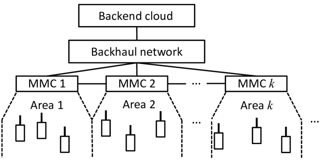
Figure 1: Application scenario.

One important issue in MMCs is to decide which MMC should perform the computation for a particular user or a set of users, taking into account user mobility and other dynamic changes in the network. Providing a service to a user (or a set of users) requires starting a service instance, which can be run either in the backend cloud or in one of the MMCs, and the question is how to choose the optimal location to run the service instance. Besides, users may move across different geographical areas due to mobility, thus another question is whether we should migrate the service instance from one cloud (which can be either an MMC or the backend cloud) to another cloud when the user location or network condition changes. For every cloud, there is a cost associated with running the service instance in it, and there is also a cost associated with migrating the service instance from one cloud to another cloud. The placement and migration of service instances therefore needs to properly take into account this cost.

1.1 Related Work

The abovementioned problems are related to application/workload placement problems in cloud environments. Although existing work has studied such problems under complex network topologies [8, 9], they mainly focused on relatively static network conditions and fixed resource demands in a data-center environment. The presence of dynamically changing resource availability that is related to user mobility in an MMC environment has not been sufficiently considered.

When user mobility exists, it is necessary to consider real-time (live) migration of service instances. For example, it can be beneficial to migrate the instance to a location closer to the user. Only a few existing papers in the literature have studied this problem [10, 11, 12]. The main approach in [10, 11, 12] is to formulate the mobility-driven service instance migration problem as a Markov decision process (MDP). Such a formulation is suitable where the user mobility follows or can be approximated by a mobility model that can be described by a Markov chain. However, there are cases where the Markovian assumption is not valid [13]. Besides, [10, 11, 12] either do not explicitly or only heuristically consider multiple users and service instances, and they assume specific structures of the cost function that are related to the locations of users and service instances. Such cost structures may be inapplicable when the load on different MMCs are imbalanced or when we consider the backend cloud as a placement option. In addition, the existing MDP-based approaches mainly consider service instances that are constantly running in the cloud system; they do not consider instances that may arrive to and depart from the system over time.

Systems with online (and usually unpredictable) arrivals and departures have been studied in the field of online approximation algorithms [14, 15]. The goal is to design efficient algorithms (usually with polynomial time-complexity) that have reasonable competitive ratios. However, most existing work focus on problems that can be formulated as integer linear programs. Problems that have convex but non-linear objective functions have attracted attention only very recently [16, 17], where the focus is on online covering problems in which new constraints arrive over time. Our problem is different from the existing work in the sense that the online arrivals in our problem are abstracted as change in constraints (or, with a slightly different but equivalent formulation, adding new variables) instead of adding new constraints, and we consider the average cost over multiple timeslots. Meanwhile, online departures are not considered in [16, 17].

Concurrently with the work presented in this paper, we have considered non-realtime applications in [18], where users submit job requests that can be processed after some time. Different from [18], we consider users continuously connected to services in this paper, which is often the case for delay-sensitive applications (such as live video streaming). The technical approach in this paper is fundamentally different from that in [18]. Besides, a Markovian mobility model is still assumed in [18].

Another related problem is the load balancing in distributed systems, where the goal is to even out the load distribution across machines. Migration cost, future cost parameter prediction and the impact of prediction error are not considered in load balancing problems [9, 19, 20, 21, 22]. We consider all these aspects in this paper, and in addition, we consider a generic cost definition that can be defined to favor load balancing as well as other aspects.

We also note that existing online algorithms with provable performance guarantees are often of theoretical nature [14, 15, 16, 17], which may not be straightforward to apply in practical systems because these algorithms can be conceptually complex thus difficult to understand. At the same time, most online algorithms applied in practice are of heuristic nature without theoretically provable optimality guarantees [8]; the performance of such algorithms are usually evaluated under a specific experimentation setting (see references of [8]), thus they may perform poorly under other settings that possibly occur in practice [23]. For example, in the machine scheduling problem considered in [24], a greedy algorithm (which is a common heuristic) that works well in some cases does not work well in other cases. We propose a simple and practically applicable online algorithm with theoretically provable performance guarantees in this paper, and also verify its performance with simulation using both synthetic arrivals and real-world user traces.

1.2 Main Contributions

In this paper, we consider a general setting which allows heterogeneity in cost values, network structure, and mobility models. We assume that the cost is related to a finite set of parameters, which can include the locations and preferences of users, load in the system, database locations, etc. We focus on the case where there is an underlying mechanism to predict the future values of these parameters, and also assume that the prediction mechanism provides the most likely future values and an upper bound on possible deviation of the actual value from the predicted value. Such an assumption is valid for many prediction methods that provide guarantees on prediction accuracy. Based on the predicted parameters, the (predicted) future costs of each configuration can be found, in which each configuration represents one particular placement sequence of service instances.

With the above assumption, we formulate a problem of finding the optimal configuration of service instances that minimizes the average cost over time. We define a look-ahead window to specify the amount of time that we look (predict) into the future. The main contributions of this paper are summarized as follows:

1. We first focus on the offline problem of service instance placement using predicted costs within a specific look-ahead window, where the instance arrivals and departures within this look-ahead window are assumed to be known beforehand. We show that this problem is equivalent to a shortest-path problem in a virtual graph formed by all possible configurations, and propose an algorithm (Algorithm 2 in Section 3.3) to find its optimal solution using dynamic programming.

2. We note that it is often practically infeasible to know in advance about when an instance will arrive to or depart from the system. Meanwhile, Algorithm 2 may have exponential time-complexity when there exist multiple instances. Therefore, we propose an online approximation algorithm that finds the placement of a service instance upon its arrival with polynomial time-complexity. The proposed online algorithm calls Algorithm 2 as a subroutine for each instance upon its arrival. We analytically evaluate the performance of this online algorithm compared to the optimal offline placement. The proposed online algorithm is $O(1)$-competitive for certain types of cost functions (including those which are linear, polynomial, or in some other specific form), under some mild assumptions.

3. Considering the existence of prediction errors, we propose a method to find the optimal look-ahead window size, such that an upper bound on the actual placement cost is minimized.

4. The effectiveness of the proposed approach is evaluated by simulations with both synthetic traces and real-world mobility traces of San Francisco taxis.

The remainder of this paper is organized as follows. The problem formulation is described in Section 2. Section 3 proposes an offline algorithm to find the optimal sequence of service instance placement with given look-ahead window size. The online placement algorithm and its performance analysis are presented in Section 4. Section 5 proposes a method to find the optimal look-ahead window size. Section 6 presents the simulation results and Section 7 draws conclusions.

2 Problem Formulation

We consider a cloud computing system as shown in Fig. 1, where the clouds are indexed by $k\in\{1,2,...,K\}$. Each cloud $k$ can be either an MMC or a backend cloud. All MMCs together with the backend cloud can host service instances that may arrive and leave the system over time. A service instance is a process that is executed for a particular task of a cloud service. Each service instance may serve one or a group users, where there usually exists data transfer between the instance and the users it is serving. A time-slotted system as shown in Fig. 2 is considered, in which the actual physical time interval corresponding to each slot $t=1,2,3,...$ can be either the same or different.

We consider a window-based control framework, where every $T$ slots, a controller performs cost prediction and computes the service instance configuration for the next $T$ slots. We define these $T$ consecutive slots as a look-ahead window. Service instance placement within each window is found either at the beginning of the window (in the offline case) or whenever an instance arrives (in the online case). We limit ourselves to within one look-ahead window when finding the configuration. In other words, we do not attempt to find the placement in the next window until the time for the current window has elapsed and the next window starts. Our solution can also be extended to a slot-based control framework where the controller computes the next $T$-slot configuration at the beginning of every slot, based on predicted cost parameters for the next $T$ slots. We leave the detailed comparison of these frameworks and their variations for future work.

Figure 2: Timing of the proposed approach.

2.1 Definitions

We introduce some definitions in the following. A summary of main notations is given in Appendix A.

2.1.1 Service Instances

We say a service instance arrives to the system if it is created, and we say it departs from the system if its operation is finished. Service instances may arrive and depart over time. We keep an index counter to assign an index for each new instance. The counter is initialized to zero when the cloud system starts to operate. Upon a service instance arrival, we increment the counter by one, so that if the previously arrived instance has index $i$, a newly arrived instance will have index $i+1$. With this definition, if $i<i^{\prime}$, instance $i$ arrives no later than instance $i^{\prime}$. A particular instance $i$ can only arrive to the system once, and we assume that arrivals always occur at the beginning of a slot and departures always occur at the end of a slot. For example, consider timeslots $t=1,2,3,4,5$, instance $i=2$ may arrive to the system at the beginning of slot $t=2$, and depart from the system at the end of slot $t=4$. At any timeslot $t$, instance $i$ can have one of the following states: not arrived, running, or departed. For the above example, instance $i=2$ has not yet arrived to the system in slot $t=1$, it is running in slots $t=2,3,4$, and it has already departed in slot $t=5$. Note that an instance can be running across multiple windows each containing $T$ slots before it departs.

2.1.2 Service Configurations

Consider an arbitrary sequence of consecutive timeslots $t\in\{t_{0},t_{0}+1,...,t_{0}+Q-1\}$, where $Q$ is an integer. For simplicity, assume that the instance with the smallest index running in slot $t_{0}$ has index $i=1$, and the instance with the largest index running in any of the slots in $\{t_{0},...,t_{0}+Q-1\}$ has index $M$. According to the index assignment discussed in Section 2.1.1, there can be at most $M$ instances running in any slot $t\in\{t_{0},...,t_{0}+Q-1\}$.

We define a $Q$-by-$M$ matrix denoted by $\bm{\pi}$, where its $(q,i)$th ($q\in\{1,...,Q\}$) element $(\bm{\pi})_{qi}\in\{0,1,2,...,K\}$ denotes the location of service instance $i$ in slot $t_{q}\triangleq t_{0}+q-1$ ( “$\triangleq$” stands for “is defined to be equal to”). We set $(\bm{\pi})_{qi}$ according to the state of instance $i$ in slot $t_{q}$, as follows

$$(\bm{\pi})_{qi}=\begin{cases}0,&\textrm{if }i\textrm{ is not running in slot }t_{q}\\ k,&\textrm{if }i\textrm{ is running in cloud }k\textrm{ in slot }t_{q}\end{cases}$$

where instance $i$ is not running if it has not yet arrived or has already departed. The matrix $\bm{\pi}$ is called the configuration of instances in slots $\{t_{0},...,t_{0}+Q-1\}$. Throughout this paper, we use matrix $\bm{\pi}$ to represent configurations in different subsets of timeslots. We write $\bm{\pi}(t_{0},t_{1},...,t_{n})$ to explicitly denote the configuration in slots $\{t_{0},t_{1},...,t_{n}\}$ (we have $Q=t_{n}-t_{0}+1$), and we write $\bm{\pi}$ for short where the considered slots can be inferred from the context. For a single slot $t$, $\bm{\pi}(t)$ becomes a vector (i.e., $Q=1$).

Remark: The configurations in different slots can appear either in the same matrix or in different matrices. This means, from $\bm{\pi}(t_{0},...,t_{0}+Q-1)$, we can get $\bm{\pi}(t)$ for any $t\in\{t_{0},...,t_{0}+Q-1\}$, as well as $\bm{\pi}(t-1,t)$ for any $t\in\{t_{0}+1,...,t_{0}+Q-1\}$, etc., and vice versa. For the ease of presentation later, we define $(\bm{\pi}(0))_{i}=0$ for any $i$.

2.1.3 Costs

The cost can stand for different performance-related factors in practice, such as monetary cost (expressed as the price in some currency), service access latency of users (in seconds), service interruption time (in seconds), amount of transmission/processing resource consumption (in the number of bits to transfer, CPU cycles, memory size, etc.), or a combination of these. As long as these aspects can be expressed in some form of a cost function, we can treat them in the same optimization framework, thus we use the generic notion of cost in this paper.

We consider two types of costs. The local cost $U(t,\bm{\pi}(t))$ specifies the cost of data transmission (e.g., between each pair of user and service instance) and processing in slot $t$ when the configuration in slot $t$ is $\bm{\pi}(t)$. Its value can depend on many factors, including user location, network condition, load of clouds, etc., as discussed in Section 1.2. When a service instance is initiated in slot $t$, the local cost in slot $t$ also includes the cost of initial placement of the corresponding service instance(s). We then define the migration cost $W(t,\bm{\pi}(t-1),\bm{\pi}(t))$, which specifies the cost related to migration between slots $t-1$ and $t$, which respectively have configurations $\bm{\pi}(t-1)$ and $\bm{\pi}(t)$. There is no migration cost in the very first timeslot (start of the system), thus we define $W(1,\cdot,\cdot)=0$. The sum of local and migration costs in slot $t$ when following configuration $\bm{\pi}(t-1,t)$ is given by

$$C_{\bm{\pi}(t-1,t)}(t)\triangleq U(t,\bm{\pi}(t))+W(t,\bm{\pi}(t-1),\bm{\pi}(t))$$ (1)

The above defined costs are aggregated costs for all service instances in the system during slot $t$. We will give concrete examples of these costs later in Section 4.2.1.

2.2 Actual and Predicted Costs

To distinguish between the actual and predicted cost values, for a given configuration $\bm{\pi}$, we let $A_{\bm{\pi}}(t)$ denote the actual value of $C_{\bm{\pi}}(t)$, and let $D_{\bm{\pi}}^{t_{0}}(t)$ denote the predicted (most likely) value of $C_{\bm{\pi}}(t)$, when cost-parameter prediction is performed at the beginning of slot $t_{0}$. For completeness of notations, we define $D_{\bm{\pi}}^{t_{0}}(t)=A_{\bm{\pi}}(t)$ for $t<t_{0}$, because at the beginning of $t_{0}$, the costs of all past timeslots are known. For $t\geq t_{0}$, we assume that the absolute difference between $A_{\bm{\pi}}(t)$ and $D_{\bm{\pi}}^{t_{0}}(t)$ is at most

$$\epsilon(\tau)\triangleq\max_{\bm{\pi},t_{0}}\left|A_{\bm{\pi}}(t_{0}+\tau)-D_{\bm{\pi}}^{t_{0}}(t_{0}+\tau)\right|$$

which represents the maximum error when looking ahead for $\tau$ slots, among all possible configurations $\bm{\pi}$ (note that only $\bm{\pi}(t_{0}+\tau-1)$ and $\bm{\pi}(t_{0}+\tau)$ are relevant) and all possible prediction time instant $t_{0}$. The function $\epsilon(\tau)$ is assumed to be non-decreasing with $\tau$, because we generally cannot have lower error when we look farther ahead into the future. The specific value of $\epsilon(\tau)$ is assumed to be provided by the cost prediction module.

We note that specific methods for predicting future cost parameters are beyond the scope of this paper, but we anticipate that existing approaches such as [25], [26] and [27] can be applied. For example, one simple approach is to measure cost parameters on the current network condition, and regard them as parameters for the future cost until the next measurement is taken. The prediction accuracy in this case is related to how fast the cost parameters vary, which can be estimated from historical records. We regard these cost parameters as predictable because they are generally related to the overall state of the system or historical pattern of users, which are unlikely to vary significantly from its previous state or pattern within a short time. This is different from arrivals and departures of instances, which can be spontaneous and unlikely to follow a predictable pattern.

2.3 Our Goal

Our ultimate goal is to find the optimal configuration $\bm{\pi}^{*}(1,...,\infty)$ that minimizes the actual average cost over a sufficiently long time, i.e.

$$\bm{\pi}^{*}(1,...,\infty)\!=\!\arg\!\!\min_{\bm{\pi}(1,...,\infty)}\lim_{T_{\textrm{max}}\rightarrow\infty}\frac{\sum_{t=1}^{T_{\textrm{max}}}A_{\bm{\pi}(t-1,t)}(t)}{T_{\textrm{max}}}$$ (2)

However, it is impractical to find the optimal solution to (2), because we cannot precisely predict the future costs and also do not have exact knowledge on instance arrival and departure events in the future. Therefore, we focus on obtaining an approximate solution to (2) by utilizing predicted cost values that are collected every $T$ slots.

Now, the service placement problem includes two parts: one is finding the look-ahead window size $T$, discussed in Section 5; the other is finding the configuration within each window, where we consider both offline and online placements, discussed in Sections 3 (offline placement) and 4 (online placement). The offline placement assumes that at the beginning of window $T$, we know the exact arrival and departure times of each instance within the rest of window $T$, whereas the online placement does not assume this knowledge. We note that the notion of “offline” here does not imply exact knowledge of future costs. Both offline and online placements in Sections 3 and 4 are based on the predicted costs $D_{\bm{\pi}}^{t_{0}}(t)$, the actual cost $A_{\bm{\pi}}(t)$ is considered later in Section 5.

3 Offline Service Placement with Given Look-Ahead Window Size

In this section, we focus on the offline placement problem, where the arrival and departure times of future instances are assumed to be exactly known. We denote the configuration found for this problem by $\bm{\pi}_{\textrm{off}}$.

3.1 Procedure

We start with illustrating the high-level procedure of finding $\bm{\pi}_{\textrm{off}}$. When the look-ahead window size $T$ is given, the configuration $\bm{\pi}_{\textrm{off}}$ is found sequentially for each window (containing timeslots $t_{0},...,t_{0}+T-1$), by solving the following optimization problem:

$$\bm{\pi}_{\textrm{off}}(t_{0},...,t_{0}\!+\!T\!-\!1)=\arg\!\!\min_{\bm{\pi}(t_{0},...,t_{0}+T-1)}\!\!\sum_{t=t_{0}}^{t_{0}+T-1}D_{\bm{\pi}(t-1,t)}^{t_{0}}(t)$$ (3)

where $D_{\bm{\pi}}^{t_{0}}(t)$ can be found based on the parameters obtained from the cost prediction module. The procedure is shown in Algorithm 1.

In Algorithm 1, every time when solving (3), we get the value of $\bm{\pi}_{\textrm{off}}$ for additional $T$ slots. This is sufficient in practice (compared to an alternative approach that directly solves for $\bm{\pi}_{\textrm{off}}$ for all slots) because we only need to know where to place the instances in the current slot. The value of $D_{\bm{\pi}(t-1,t)}^{t_{0}}(t)$ in (3) depends on the configuration in slot $t_{0}-1$, i.e. $\bm{\pi}(t_{0}-1)$, according to (1). When $t_{0}=1$, $\bm{\pi}(t_{0}-1)$ can be regarded as an arbitrary value, because the migration cost $W(t,\cdot,\cdot)=0$ for $t=1$.

Intuitively, at the beginning of slot $t_{0}$, (3) finds the optimal configuration that minimizes the predicted cost over the next $T$ slots, given the locations of instances in slot $t_{0}-1$. We focus on solving (3) next.

Algorithm 1 Procedure of offline service placement

1:  Initialize $t_{0}=1$

2:  loop

3:     At the beginning of slot $t_{0}$, find the solution to (3)

4:     Apply placements $\bm{\pi}_{\textrm{off}}(t_{0},...,t_{0}+T-1)$ in timeslots $t_{0},...,t_{0}+T-1$

5:     $t_{0}\leftarrow t_{0}+T$

6:  end loop

3.2 Equivalence to Shortest-Path Problem

The problem in (3) is equivalent to a shortest-path problem with $D_{\bm{\pi}(t-1,t)}^{t_{0}}(t)$ as weights, as shown in Fig. 3. Each edge represents one possible combination of configurations in adjacent timeslots, and the weight on each edge is the predicted cost for such configurations. The configuration in slot $t_{0}-1$ is always given, and the number of possible configurations in subsequent timeslots is at most $K^{M}$, where $M$ is defined as in Section 2.1.2 for the current window $\{t_{0},...,t_{0}+T-1\}$, and we note that depending on whether the instance is running in the system or not, the number of possible configurations in a slot is either $K$ or one (for configuration $0$). Node B is a dummy node to ensure that we find a single shortest path, and the edges connecting node B have zero weights. It is obvious that the optimal solution to (3) can be found by taking the shortest (minimum-weighted) path from node $\bm{\pi}(t_{0}-1)$ to node B in Fig. 3; the nodes that the shortest path traverses correspond to the optimal solution $\bm{\pi}_{\textrm{off}}(t_{0},...,t_{0}+T-1)$ for (3).

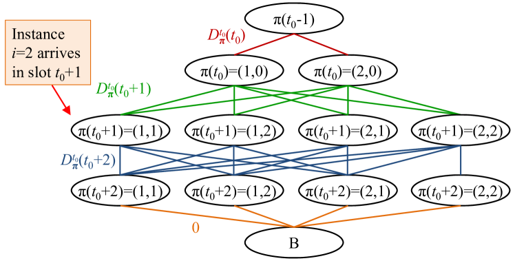
Figure 3: Shortest-path formulation with $K=2$, $M=2$, and $T=3$. Instance $i=1$ is running in all slots, instance $i=2$ arrives at the beginning of slot $t_{0}+1$ and is running in slots $t_{0}+1$ and $t_{0}+2$.

3.3 Algorithm

We can solve the abovementioned shortest-path problem by means of dynamic programming [28]. The algorithm is shown in Algorithm 2, where we use $U_{p}(t,\mathbf{m})$ and $W_{p}(t,\mathbf{n},\mathbf{m})$ to respectively denote the predicted local and migration costs when $\bm{\pi}(t)=\mathbf{m}$ and $\bm{\pi}(t-1)=\mathbf{n}$.

In the algorithm, Lines 5–16 iteratively find the shortest path (minimum objective function) for each timeslot. The iteration starts from the second level of the virtual graph in Fig. 3, which contains nodes with $\pi(t_{0})$. It iterates through all the subsequent levels that respectively contain nodes with $\pi(t_{0}+1)$, $\pi(t_{0}+2)$, etc., excluding the last level with node B. In each iteration, the optimal solution for every possible (single-slot) configuration $\mathbf{m}$ is found by solving the Bellman’s equation of the problem (Line 11). Essentially, the Bellman’s equation finds the shortest path between the top node $\pi(t_{0}-1)$ and the current node under consideration (e.g., node $\pi(t_{0}+1)=(1,1)$ in Fig. 3), by considering all the nodes in the previous level (nodes $\pi(t_{0})=(1,0)$ and $\pi(t_{0})=(2,0)$ in Fig. 3). The sum weight on the shortest path between each node in the previous level and the top node $\pi(t_{0}-1)$ is stored in $\nu_{\mathbf{m}}$, and the corresponding nodes that this shortest path traverses through is stored in $\bm{\xi}_{\mathbf{m}}$. Based on $\nu_{\mathbf{m}}$ and $\bm{\xi}_{\mathbf{m}}$, Line 11 finds the shortest paths for all nodes in the current level, which can again be used for finding the shortest paths for all nodes in the next level (in the next iteration).

After iterating through all levels, the algorithm has found the shortest paths between top node $\pi(t_{0}-1)$ and all nodes in the last level with $\pi(t_{0}-T-1)$. Now, Lines 17 and 18 find the minimum of all these shortest paths, giving the optimal configuration. It is obvious that output of this algorithm satisfies the Bellman’s principle of optimality, so the result is the shortest path and hence the optimal solution to (3).

Complexity: When the vectors $\bm{\pi}_{\mathbf{m}}$ and $\bm{\xi}_{\mathbf{m}}$ are stored as linked-lists, Algorithm 2 has time-complexity $O\left(K^{2M}T\right)$, because the minimization in Line 11 requires enumerating at most $K^{M}$ possible configurations, and there can be at most $K^{M}T$ possible combinations of values of $t$ and $\mathbf{m}$.

Algorithm 2 Algorithm for solving (3)

1:  Define variables $\mathbf{m}$ and $\mathbf{n}$ to represent configurations respectively in the current and previous iteration (level of graph)

2:  Define vectors $\bm{\pi}_{\mathbf{m}}$ and $\bm{\xi}_{\mathbf{m}}$ for all $\mathbf{m},\mathbf{n}$, where $\bm{\pi}_{\mathbf{m}}$ (correspondingly, $\bm{\xi}_{\mathbf{m}}$) records the optimal configuration given that the configuration at the current (correspondingly, previous) timeslot of iteration is $\mathbf{m}$

3:  Define variables $\mu_{\mathbf{m}}$ and $\nu_{\mathbf{m}}$ for all $\mathbf{m}$ to record the sum cost values from slot $t_{0}$ respectively to the current and previous slot of iteration, given that the configuration is $\mathbf{m}$ in the current or previous slot

4:  Initialize $\mu_{\mathbf{m}}\leftarrow 0$ and $\bm{\pi}_{\mathbf{m}}\leftarrow\emptyset$ for all $\mathbf{m}$

5:  for $t=t_{0},...,t_{0}+T-1$ do

6:     for all $\mathbf{m}$ do

7:        $\nu_{\mathbf{m}}\leftarrow\mu_{\mathbf{m}}$

8:        $\bm{\xi}_{\mathbf{m}}\leftarrow\bm{\pi}_{\mathbf{m}}$

9:     end for

10:     for all $\mathbf{m}$ do

11:        $\mathbf{n}^{*}\leftarrow\arg\min_{\mathbf{n}}\left\{\nu_{\mathbf{n}}+U_{p}(t,\mathbf{m})+W_{p}(t,\mathbf{n},\mathbf{m})\right\}$

12:        $\bm{\pi}_{\mathbf{m}}(t_{0},...,t-1)\leftarrow\bm{\xi}_{\mathbf{n}^{*}}(t_{0},...,t-1)$

13:        ${\pi}_{\mathbf{m}}(t)\leftarrow\mathbf{m}$

14:        $\mu_{\mathbf{m}}\leftarrow\nu_{\mathbf{n}^{*}}+U_{p}(t,\mathbf{m})+W_{p}(t,\mathbf{n}^{*},\mathbf{m})$

15:     end for

16:  end for

17:  $\mathbf{m}^{*}\leftarrow\arg\min_{\mathbf{m}}\mu_{\mathbf{m}}$

18:  $\bm{\pi}_{\textrm{off}}(t_{0},...,t_{0}+T-1)\leftarrow\bm{\pi}_{\mathbf{m}^{*}}(t_{0},...,t_{0}+T-1)$

19:  return  $\bm{\pi}_{\textrm{off}}(t_{0},...,t_{0}+T-1)$

4 Complexity Reduction and Online Service Placement

The complexity of Algorithm 2 is exponential in the number of instances $M$, so it is desirable to reduce the complexity. In this section, we propose a method that can find an approximate solution to (3) and, at the same time, handle online instance arrivals and departures that are not known beforehand. We will also show that (3) is NP-hard when $M$ is non-constant, which justifies the need to solve (3) approximately in an efficient manner.

4.1 Procedure

In the online case, we modify the procedure given in Algorithm 1 so that instances are placed one-by-one, where each placement greedily minimizes the objective function given in (3), while the configurations of previously placed instances remain unchanged.

We assume that each service instance $i$ has a maximum lifetime $T_{\textrm{life}}(i)$, denoting the maximum number of remaining timeslots (including the current slot) that the instance remains in the system. The value of $T_{\textrm{life}}(i)$ may be infinity for instances that can potentially stay in the system for an arbitrary amount of time. The actual time that the instance stays in the system may be shorter than $T_{\textrm{life}}(i)$, but it cannot be longer than $T_{\textrm{life}}(i)$. When an instance leaves the system before its maximum lifetime has elapsed, we say that such a service instance departure is unpredictable.

We use $\bm{\pi}_{\textrm{on}}$ to denote the configuration $\bm{\pi}$ computed by online placement. The configuration $\bm{\pi}_{\textrm{on}}$ is updated every time when an instance arrives or unpredictably departs. At the beginning of the window (before any instance has arrived), it is initiated as an all-zero matrix.

For a specific look-ahead window $\{t_{0},...,t_{0}+T-1\}$, when service instance $i$ arrives in slot $t\in\{t_{0},...,t_{0}+T-1\}$, we assume that this instance stays in the system until slot $t_{e}=\min\left\{t+T_{\textrm{life}}(i)-1;t_{0}+T-1\right\}$, and accordingly update the configuration by

$$\bm{\pi}_{\textrm{on}}(t,...,t_{e})=\arg\min_{\bm{\pi}(t_{a},...,t_{e})}\sum_{t=t_{a}}^{t_{e}}D_{\bm{\pi}(t-1,t)}^{t_{0}}(t)$$ (4)

$$\textrm{s.t.}\>\bm{\pi}(t,...,t_{e})=\bm{\pi}_{\textrm{on}}(t,...,t_{e})\textrm{ except for column }i$$

Note that only the configuration of instance $i$ (which is assumed to be stored in the $i$th column of $\bm{\pi}$) is found and updated in (4), the configurations of all other instances $i^{\prime}\neq i$ remain unchanged. The solution to (4) can still be found with Algorithm 2. The only difference is that vectors $\mathbf{m}$ and $\mathbf{n}$ now become scalar values within $\{1,...,K\}$, because we only consider the configuration of a single instance $i$. The complexity in this case becomes $O(K^{2}T)$. At the beginning of the window, all the instances that have not departed after slot $t_{0}-1$ are seen as arrivals in slot $t_{0}$, because we independently consider the placements in each window of size $T$. When multiple instances arrive simultaneously, an arbitrary arrival sequence is assigned to them; the instances are still placed one-by-one by greedily minimizing (4).

When an instance $i$ unpredictably departs at the end of slot $t\in\{t_{0},...,t_{0}+T-1\}$, we update $\bm{\pi}_{\textrm{on}}$ such that the $i$th column of $\bm{\pi}_{\textrm{on}}(t+1,...,t_{0}+T-1)$ is set to zero.

The online procedure described above is shown in Algorithm 3. Recall that $\bm{\pi}_{\textrm{on}}(t,...,t_{e})$ and $\bm{\pi}_{\textrm{on}}(t+1,...,t_{0}+T-1)$ are both part of a larger configuration matrix $\bm{\pi}_{\textrm{on}}(t_{0},...,t_{0}+T-1)$ (see Section 2.1.2).

Complexity: When placing a total of $M$ instances, for a specific look-ahead window with size $T$, we can find the configurations of these $M$ instances with complexity $O(K^{2}TM)$, because (4) is solved for $M$ times, each with complexity $O(K^{2}T)$.

Algorithm 3 Procedure of online service placement

1:  Initialize $t_{0}=1$

2:  loop

3:     Initialize $\bm{\pi}_{\textrm{on}}(t_{0},...,t_{0}+T-1)$ as an all-zero matrix

4:     for each timeslot $t=t_{0},...,t_{0}+T-1$ do

5:        for each instance $i$ arriving at the beginning of slot $t$ do

6:           $t_{e}\leftarrow\min\left\{t+T_{\textrm{life}}(i)-1;t_{0}+T-1\right\}$

7:           Update $\bm{\pi}_{\textrm{on}}(t,...,t_{e})$ with the result from (4)

8:           Apply configurations specified in the $i$th column of $\bm{\pi}_{\textrm{on}}(t,...,t_{e})$ for service instance $i$ in timeslots $t,...,t_{e}$ until instance $i$ departs

9:        end for

10:        for each instance $i$ departing at the end of slot $t$ do

11:            Set the $i$th column of $\bm{\pi}_{\textrm{on}}(t+1,...,t_{0}+T-1)$ to zero

12:        end for

13:     end for

14:     $t_{0}\leftarrow t_{0}+T$

15:  end loop

Remark: It is important to note that in the above procedure, the configuration $\bm{\pi}_{\textrm{on}}$ (and thus the cost value $D_{\bm{\pi}(t-1,t)}^{t_{0}}(t)$ for any $t\in\{t_{0},...,t_{0}+T-1\}$) may vary upon instance arrival or departure. It follows that the $T$-slot sum cost $\sum_{t=t_{0}}^{t_{0}+T-1}D_{\bm{\pi}_{\textrm{on}}(t-1,t)}^{t_{0}}(t)$ may vary whenever an instance arrives or departs at an arbitrary slot $t\in\{t_{0},...,t_{0}+T-1\}$, and the value of $\sum_{t=t_{0}}^{t_{0}+T-1}D_{\bm{\pi}_{\textrm{on}}(t-1,t)}^{t_{0}}(t)$ stands for the predicted sum cost (over the current window containing $T$ slots) under the current configuration, assuming that no new instance arrives and no instance unpredictably departs in the future. This variation in configuration and cost upon instance arrival/departure is frequently mentioned in the analysis presented next.

4.2 Performance Analysis

It is clear that for a single look-ahead window, Algorithm 3 has polynomial time-complexity while Algorithm 1 has exponential time-complexity. In this subsection, we show the NP-hardness of the offline service placement problem, and discuss the optimality gap between the online algorithm and the optimal offline placement. Note that we only focus on a single look-ahead window in this subsection. The interplay of multiple look-ahead windows and the impact of the window size will be considered in Section 5.

4.2.1 Definitions

For simplicity, we analyze the performance for a slightly restricted (but still general) class of cost functions. We introduce some additional definitions next (see Appendix A for a summary of notations).

Indexing of Instances: Here, we assume that the instance with lowest index in the current window $\{t_{0},...,t_{0}+T-1\}$ has index $i=1$, and the last instance that arrives before the current time of interest has index $i=M$, where the current time of interest can be any time within the current window. With this definition, $M$ does not need to be the largest index in window $\{t_{0},...,t_{0}+T-1\}$. Instead, it can be the index of any instance that arrives within $\{t_{0},...,t_{0}+T-1\}$. The cost of placing up to (and including) instance $M$ is considered, where some instances $i\leq M$ may have already departed from the system.

Possible Configuration Sequence: When considering a window of $T$ slots, we define the set of all possible configurations of a single instance as a set of $T$-dimensional vectors $\Lambda\triangleq\{\left(\lambda_{1},...,\lambda_{T}\right):\lambda_{n}\in\{0,1,...,K\},\forall n\in\{1,...,T\},$ where $\lambda_{n}$ is non-zero for at most one block of consecutive values of $n\}$. We also define a vector $\bm{\lambda}\in\Lambda$ to represent one possible configuration sequence of a single service instance across these $T$ consecutive slots. For any instance $i$, the $i$th column of configuration matrix $\bm{\pi}(t_{0},...,t_{0}+T-1)$ is equal to one particular value of $\bm{\lambda}$.

We also define a binary variable $x_{i\bm{\lambda}}$, where $x_{i\bm{\lambda}}=1$ if instance $i$ is placed according to configuration sequence $\bm{\lambda}$ across slots $\{t_{0},...,t_{0}+T-1\}$ (i.e., the $i$th column of $\bm{\pi}(t_{0},...,t_{0}+T-1)$ is equal to $\bm{\lambda}$), and $x_{i\bm{\lambda}}=0$ otherwise. We always have $\sum_{\bm{\lambda}\in\Lambda}x_{i\bm{\lambda}}=1$ for all $i\in\{1,...,M\}$.

We note that the values of $x_{i\bm{\lambda}}$ may vary over time due to arrivals and unpredictable departures of instances, which can be seen from Algorithm 3 and by noting the relationship between $\bm{\lambda}$ and $\bm{\pi}$. Before instance $i$ arrives, $x_{i\bm{\lambda}_{0}}=1$ for $\bm{\lambda}_{0}=[0,...,0]$ which contains all zeros, and $x_{i\bm{\lambda}}=0$ for $\bm{\lambda}\neq\bm{\lambda}_{0}$. Upon arrival of instance $i$, we have $x_{i\bm{\lambda}_{0}}=0$ and $x_{i\bm{\lambda}_{1}}=1$ for a particular $\bm{\lambda}_{1}$. When instance $i$ unpredictably departs at slot $t^{\prime}$, its configuration sequence switches from $\bm{\lambda}_{1}$ to an alternative (but partly correlated) sequence $\bm{\lambda}^{\prime}_{1}$ (i.e., $(\bm{\lambda}^{\prime}_{1})_{t}=(\bm{\lambda}_{1})_{t}$ for $t\leq t^{\prime}$ and $(\bm{\lambda}^{\prime}_{1})_{t}=0$ for $t>t^{\prime}$, where $(\bm{\lambda})_{t}$ denotes the $t$th element of $\bm{\lambda}$), according to Line 11 in Algorithm 3, after which $x_{i\bm{\lambda}_{1}}=0$ and $x_{i\bm{\lambda}^{\prime}_{1}}=1$.

Resource Consumption: We assume that the costs are related to the resource consumption, and for the ease of presentation, we consider two types of resource consumptions. The first type is associated with serving user requests, i.e., data transmission and processing when a cloud is running a service instance, which we refer to as the local resource consumption. The second type is associated with migration, i.e., migrating an instance from one cloud to another cloud, which we refer to as the migration resource consumption.

If we know that instance $i$ operates under configuration sequence $\bm{\lambda}$, then we know whether instance $i$ is placed on cloud $k$ in slot $t$, for any $k\in\{1,...,K\}$ and $t\in\{t_{0},...,t_{0}+T-1\}$. We also know whether instance $i$ is migrated from cloud $k$ to cloud $l$ ($l\in\{1,2,...,K\}$) between slots $t-1$ and $t$. We use $a_{i\bm{\lambda}k}(t)\geq 0$ to denote the local resource consumption at cloud $k$ in slot $t$ when instance $i$ is operating under $\bm{\lambda}$, where $a_{i\bm{\lambda}k}(t)=0$ if $(\bm{\lambda})_{t}\neq k$. We use $b_{i\bm{\lambda}kl}(t)\geq 0$ to denote the migration resource consumption when instance $i$ operating under $\bm{\lambda}$ is assigned to cloud $k$ in slot $t-1$ and to cloud $l$ in slot $t$, where $b_{i\bm{\lambda}kl}(t)=0$ if $(\bm{\lambda})_{t-1}\neq k$ or $(\bm{\lambda})_{t}\neq l$, and we note that the configuration in slot $t_{0}-1$ (before the start of the current window) is assumed to be given and thus independent of $\bm{\lambda}$. The values of $a_{i\bm{\lambda}k}(t)$ and $b_{i\bm{\lambda}kl}(t)$ are either service-specific parameters that are known beforehand, or they can be found as part of the cost prediction.

We denote the sum local resource consumption at cloud $k$ by $y_{k}(t)\triangleq\sum_{i=1}^{M}\sum_{\bm{\lambda}\in\Lambda}a_{i\bm{\lambda}k}(t)x_{i\bm{\lambda}}$, and denote the sum migration resource consumption from cloud $k$ to cloud $l$ by $z_{kl}(t)\triangleq\sum_{i=1}^{M}\sum_{\bm{\lambda}\in\Lambda}b_{i\bm{\lambda}kl}(t)x_{i\bm{\lambda}}$. We may omit the argument $t$ in the following discussion.

Remark: The local and migration resource consumptions defined above can be related to CPU and communication bandwidth occupation, etc., or the sum of them. We only consider these two types of resource consumption for the ease of presentation. By applying the same theoretical framework, the performance gap results (presented later) can be extended to incorporate multiple types of resources and more sophisticated cost functions, and similar results yield for the general case.

Costs: We refine the costs defined in Section 2.1.3 by considering the cost for each cloud or each pair of clouds. The local cost at cloud $k$ in timeslot $t$ is denoted by $u_{k,t}\left(y_{k}(t)\right)$. When an instance is initiated in slot $t$, the local cost in slot $t$ also includes the cost of initial placement of the corresponding instance. The migration cost from cloud $k$ to cloud $l$ between slots $t-1$ and $t$ is denoted by $w_{kl,t}\left(y_{k}(t-1),y_{l}(t),z_{kl}(t)\right)$. Besides $z_{kl}(t)$, the migration cost is also related to $y_{k}(t-1)$ and $y_{l}(t)$, because additional processing may be needed for migration, and the cost for such processing can be related to the current load at clouds $k$ and $l$. The functions $u_{k,t}\left(y\right)$ and $w_{kl,t}\left(y_{k},y_{l},z_{kl}\right)$ can be different for different slots $t$ and different clouds $k$ and $l$, and they can depend on many factors, such as network condition, background load of the cloud, etc. Noting that any constant term added to the cost function does not affect the optimal configuration, we set $u_{k,t}(0)=0$ and $w_{kl,t}(0,0,0)=0$. We also set $w_{kl,t}(\cdot,\cdot,0)=0$, because there is no migration cost if we do not migrate. There is also no migration cost at the start of the first timeslot, thus we set $w_{kl,t}(\cdot,\cdot,\cdot)=0$ for $t=1$. With these definitions, the aggregated costs $U(t,\bm{\pi}(t))$ and $W(t,\bm{\pi}(t-1),\bm{\pi}(t))$ can be explicitly expressed as

$$U(t,\bm{\pi}(t)) \triangleq\sum_{k=1}^{K}u_{k,t}\left(y_{k}(t)\right)$$ (5)

$$W\!(t,\bm{\pi}(t\!-\!1),\!\bm{\pi}(t))\!\! \triangleq\!\!\sum_{k=1}^{K}\!\sum_{l=1}^{K}\!w_{kl,t}\!\left(y_{k}(t\!-\!1),y_{l}(t),z_{kl}(t)\right)$$ (6)

We then assume that the following assumption is satisfied for the cost functions, which holds for a large class of practical cost functions, such as those related to the delay performance or load balancing [9].

Assumption 1.

Both $u_{k,t}(y)$ and $w_{kl,t}(y_{k},y_{l},z_{kl})$ are convex non-decreasing functions of $y$ (or $y_{k},y_{l},z_{kl}$), satisfying:

• $\frac{du_{k,t}}{dy}(0)>0$

• $\frac{\partial w_{kl,t}}{\partial z_{kl}}\left(\cdot,\cdot,0\right)>0$ for $t\geq 2$

for all $t$, $k$, and $l$ (unless stated otherwise), where $\frac{du_{k,t}}{dy}(0)$ denotes the derivative of $u_{k,t}$ with respect to (w.r.t.) $y$ evaluated at $y=0$, and $\frac{\partial w_{kl,t}}{\partial z_{kl}}\left(\cdot,\cdot,0\right)$ denotes the partial derivative of $w_{kl,t}$ w.r.t. $z_{kl}$ evaluated at $z_{kl}=0$ and arbitrary $y_{k}$ and $y_{l}$.

Vector Notation: To simplify the presentation, we use vectors to denote a collection of variables across multiple clouds, slots, or configuration sequences. For simplicity, we index each element in the vector with multiple indexes that are related to the index of the element, and use the general notion $\left(\mathbf{g}\right)_{h_{1}h_{2}}$ (or $\left(\mathbf{g}\right)_{h_{1}h_{2}h_{3}}$) to denote the $(h_{1},h_{2})$th (or $(h_{1},h_{2},h_{3})$th) element in an arbitrary vector $\mathbf{g}$. Because we know the range of each index, multiple indexes can be easily mapped to a single index. We regard each vector as a single-indexed vector for the purpose of vector concatenation (i.e., joining two vectors into one vector) and gradient computation later.

We define vectors $\mathbf{y}$ (with $KT$ elements), $\mathbf{z}$ (with $K^{2}T$ elements), $\mathbf{x}$ (with $MK^{T}$ elements), $\mathbf{a}_{i\bm{\lambda}}$ (with $KT$ elements), and $\mathbf{b}_{i\bm{\lambda}}$ (with $K^{2}T$ elements), for every value of $i\in\{1,2,...,M\}$ and $\bm{\lambda}\in\Lambda$. Different values of $i$ and $\bm{\lambda}$ correspond to different vectors $\mathbf{a}_{i\bm{\lambda}}$ and $\mathbf{b}_{i\bm{\lambda}}$. The elements in these vectors are defined as follows:

$$\left(\mathbf{y}\right)_{kt}\triangleq y_{k}(t),\>\left(\mathbf{z}\right)_{klt}\triangleq z_{kl}(t),\>\left(\mathbf{x}\right)_{i\bm{\lambda}}\triangleq x_{i\bm{\lambda}},$$

$$\left(\mathbf{a}_{i\bm{\lambda}}\right)_{kt}\triangleq a_{i\bm{\lambda}k}(t),\>\left(\mathbf{b}_{i\bm{\lambda}}\right)_{klt}\triangleq b_{i\bm{\lambda}kl}(t)$$

As discussed earlier in this section, $x_{i\bm{\lambda}}$ may unpredictably change over time due to arrivals and departures of service instances. It follows that the vectors $\mathbf{x}$, $\mathbf{y}$, and $\mathbf{z}$ may vary over time (recall that $\mathbf{y}$ and $\mathbf{z}$ are dependent on $\mathbf{x}$ by definition). The vectors $\mathbf{a}_{i\bm{\lambda}}$ and $\mathbf{b}_{i\bm{\lambda}}$ are constant.

Alternative Cost Expression: Using the above definitions, we can write the sum cost of all $T$ slots as follows

$$\widetilde{D}\left(\mathbf{x}\right)\triangleq\widetilde{D}\left(\mathbf{y},\mathbf{z}\right)\triangleq\sum_{t=t_{0}}^{t_{0}+T-1}\Bigg{[}\sum_{k=1}^{K}u_{k,t}\left(y_{k}(t)\right)$$

$$\quad\quad\quad\quad\quad+\sum_{k=1}^{K}\sum_{l=1}^{K}w_{kl,t}\left(y_{k}(t-1),y_{l}(t),z_{kl}(t)\right)\Bigg{]}$$ (7)

where the cost function $\widetilde{D}(\cdot)$ can be expressed either in terms of $\mathbf{x}$ or in terms of $\left(\mathbf{y},\mathbf{z}\right)$. The cost function defined in (7) is equivalent to $\sum_{t=t_{0}}^{t_{0}+T-1}D_{\bm{\pi}(t-1,t)}^{t_{0}}(t)$, readers are also referred to the per-slot cost defined in (1) for comparison. The value of $\widetilde{D}\left(\mathbf{x}\right)$ or, equivalently, $\widetilde{D}\left(\mathbf{y},\mathbf{z}\right)$ may vary over time due to service arrivals and unpredictable service instance departures as discussed above.

4.2.2 Equivalent Problem Formulation

With the above definitions, the offline service placement problem in (3) can be equivalently formulated as the following, where our goal is to find the optimal configuration for all service instances $1,2,...,M$ (we consider the offline case here where we know when each instance arrives and no instance will unpredictably leave after they have been placed):

$$\min_{\mathbf{x}}\quad \widetilde{D}\left(\mathbf{x}\right)$$ (8)

$$s.t.\quad \sum_{\bm{\lambda}\in\Lambda_{i}}x_{i\bm{\lambda}}=1,\forall i\in\{1,2,...,M\}$$

$$x_{i\bm{\lambda}}\in\{0,1\},\forall i\in\{1,2,...,M\},\bm{\lambda}\in\Lambda_{i}$$

where $\Lambda_{i}\subseteq\Lambda$ is a subset of feasible configuration sequences for instance $i$, i.e., sequences that contain those vectors whose elements are non-zero starting from the slot at which $i$ arrives and ending at the slot at which $i$ departs, while all other elements of the vectors are zero.

We now show that (8), and thus (3), is NP-hard even in the offline case, which further justifies the need for an approximation algorithm for solving the problem.

Proposition 1.

(NP-Hardness) The problem in (8) in the offline sense, and thus (3), is NP-hard.

Proof.

Problem (8) can be reduced from the partition problem, which is known to be NP-complete [29, Corollary 15.28]. See Appendix B for details. ∎

An online version of problem (8) can be constructed by updating $\Lambda_{i}$ over time. When an arbitrary instance $i$ has not yet arrived, we define $\Lambda_{i}$ as the set containing an all-zero vector. After instance $i$ arrives, we assume that it will run in the system until $t_{e}$ (defined in Section 4.1), and update $\Lambda_{i}$ to conform to the arrival and departure times of instance $i$ (see above). After instance $i$ departs, $\Lambda_{i}$ can be further updated so that the configurations corresponding to all remaining slots are zero.

4.2.3 Performance Gap

As discussed earlier, Algorithm 3 solves (8) in a greedy manner, where each service instance $i$ is placed to greedily minimize in (8). In the following, we compare the result from Algorithm 3 with the true optimal result, where the optimal result assumes offline placement. We use $\mathbf{x}$ and $\left(\mathbf{y},\mathbf{z}\right)$ to denote the result from Algorithm 3, and use $\mathbf{x}^{*}$ and $\left(\mathbf{y}^{*},\mathbf{z}^{*}\right)$ to denote the offline optimal result to (8).

Lemma 1.

(Convexity of $\widetilde{D}(\cdot)$) When Assumption 1 is satisfied, the cost function $\widetilde{D}\left(\mathbf{x}\right)$ or, equivalently, $\widetilde{D}\left(\mathbf{y},\mathbf{z}\right)$ is a non-decreasing convex function w.r.t. $\mathbf{x}$, and it is also a non-decreasing convex function w.r.t. $\mathbf{y}$ and $\mathbf{z}$.

Proof.

According to Assumption 1, $u_{k,t}\left(y_{k}(t)\right)$ and $w_{kl,t}\left(y_{k}(t-1),y_{l}(t),z_{kl}(t)\right)$ are non-decreasing convex functions. Because $y_{k}(t)$ and $z_{kl}(t)$ are linear mappings of $x_{i\bm{\lambda}}$ with non-negative weights for any $t$, $k$, and $l$, and also because the sum of non-decreasing convex functions is still a non-decreasing convex function, the lemma holds [30, Section 3.2].∎

In the following, we use $\nabla_{\mathbf{x}}$ to denote the gradient w.r.t. each element in vector $\mathbf{x}$, i.e., the $(i,\bm{\lambda})$th element of $\nabla_{\mathbf{x}}\widetilde{D}(\mathbf{x})$ is $\frac{\partial\widetilde{D}(\mathbf{x})}{\partial x_{i\bm{\lambda}}}$. Similarly, we use $\nabla_{\mathbf{y,z}}$ to denote the gradient w.r.t. each element in vector $(\mathbf{y,z})$, where $(\mathbf{y,z})$ is a vector that concatenates vectors $\mathbf{y}$ and $\mathbf{z}$.

Proposition 2.

(Performance Gap) When Assumption 1 is satisfied, we have

$$\widetilde{D}(\mathbf{x})\leq\widetilde{D}(\phi\psi\mathbf{x}^{*})$$ (9)

or, equivalently,

$$\widetilde{D}\left(\mathbf{y},\mathbf{z}\right)\leq\widetilde{D}\left(\phi\psi\mathbf{y}^{*},\phi\psi\mathbf{z}^{*}\right)$$ (10)

where $\phi$ and $\psi$ are constants satisfying

$$\phi\geq\frac{\nabla_{\mathbf{y,z}}\widetilde{D}\left(\mathbf{y}_{\textrm{max}}+\mathbf{a}_{i\bm{\lambda}},\mathbf{z}_{\textrm{max}}+\mathbf{b}_{i\bm{\lambda}}\right)\cdot\left(\mathbf{a}_{i\bm{\lambda}},\mathbf{b}_{i\bm{\lambda}}\right)}{\nabla_{\mathbf{y,z}}\widetilde{D}\left(\mathbf{y},\mathbf{z}\right)\cdot\left(\mathbf{a}_{i\bm{\lambda}},\mathbf{b}_{i\bm{\lambda}}\right)}$$ (11)

$$\psi\geq\frac{\nabla_{\mathbf{x}}\widetilde{D}\left(\mathbf{x}\right)\cdot\mathbf{x}}{\widetilde{D}(\mathbf{x})}=\frac{\nabla_{\mathbf{y,z}}\widetilde{D}\left(\mathbf{y},\mathbf{z}\right)\cdot\left(\mathbf{y},\mathbf{z}\right)}{\widetilde{D}\left(\mathbf{y},\mathbf{z}\right)}$$ (12)

for any $i$ and $\bm{\lambda}\in\Lambda_{i}$, in which $\mathbf{y}_{\textrm{max}}$ and $\mathbf{z}_{\textrm{max}}$ respectively denote the maximum values of $\mathbf{y}$ and $\mathbf{z}$ (the maximum is taken element-wise) after any number of instance arrivals within slots $\{t_{0},...,t_{0}+T-1\}$ until the current time of interest (at which time the latest arrived instance has index $M$), $\left(\mathbf{a}_{i\bm{\lambda}},\mathbf{b}_{i\bm{\lambda}}\right)$ is a vector that concatenates $\mathbf{a}_{i\bm{\lambda}}$ and $\mathbf{b}_{i\bm{\lambda}}$, and “$\cdot$” denotes the dot-product.

Proof.

See Appendix C. ∎

Remark: We note that according to the definition of $M$ in Section 4.2.1, the bound given in Proposition 2 holds at any time of interest within slots $\{t_{0},...,t_{0}+T-1\}$, i.e., for any number of instances that has arrived to the system, where some of them may have already departed.

4.2.4 Intuitive Explanation to the Constants $\phi$ and $\psi$

The constants $\phi$ and $\psi$ in Proposition 2 are related to “how convex” the cost function is. In other words, they are related to how fast the cost of placing a single instance changes under different amount of existing resource consumption. Figure 4 shows an illustrative example, where we only consider one cloud and one timeslot (i.e., $t=1$, $T=1$, and $K=1$). In this case, setting $\phi=\frac{d\widetilde{D}}{dy}(y_{\textrm{max}}+a_{\textrm{max}})\big{/}\frac{d\widetilde{D}}{dy}(y)$ satisfies (11), where $a_{\textrm{max}}$ denotes the maximum resource consumption of a single instance. Similarly, setting $\psi=\frac{d\widetilde{D}}{dy}(y)\cdot y\big{/}\widetilde{D}(y)$ satisfies (12). We can see that the values of $\phi$ and $\psi$ need to be larger when the cost function is more convex. For the general case, there is a weighted sum in both the numerator and denominator in (11) and (12). However, when we look at a single cloud (for the local cost) or a single pair of clouds (for the migration cost) in a single timeslot, the above intuition still applies.

So, why is the optimality gap larger when the cost functions are more convex, i.e., have a larger second order derivative? We note that in the greedy assignment procedure in Algorithm 3, we choose the configuration of each instance $i$ by minimizing the cost under the system state at the time when instance $i$ arrives, where the system state represents the local and migration resource consumptions as specified by vectors $\mathbf{y}$ and $\mathbf{z}$. When cost functions are more convex, for an alternative system state $(\mathbf{y}^{\prime},\mathbf{z}^{\prime})$, it is more likely that the placement of instance $i$ (which was determined at system state $(\mathbf{y},\mathbf{z})$) becomes far from optimum. This is because if cost functions are more convex, the cost increase of placing a new instance $i$ (assuming the same configuration for $i$) varies more when $(\mathbf{y},\mathbf{z})$ changes. This intuition is confirmed by formal results described next.

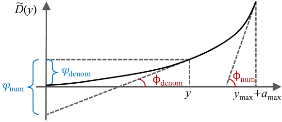
Figure 4: Illustration of the performance gap for $t=1$, $T=1$, and $K=1$, where $a_{\textrm{max}}$ denotes the maximum resource consumption of a single instance. In this example, (11) becomes $\phi\geq\frac{\phi_{\textrm{num}}}{\phi_{\textrm{denom}}}$, and (12) becomes $\psi\geq\frac{\psi_{\textrm{num}}}{\psi_{\textrm{denom}}}$.

4.2.5 Linear Cost Functions

Consider linear cost functions in the form of

$$u_{k,t}(y) =\gamma_{k,t}y$$ (13)

$$w_{kl,t}\left(y_{k},y_{l},z_{kl}\right) =\kappa_{kl,t}^{(1)}y_{k}+\kappa_{kl,t}^{(2)}y_{l}+\kappa_{kl,t}^{(3)}z_{kl}$$ (14)

where the constants $\gamma_{k,t},\kappa_{kl,t}^{(3)}>0$ and $\kappa_{kl,t}^{(1)},\kappa_{kl,t}^{(2)}\geq 0$.

Proposition 3.

When the cost functions are defined as in (13) and (14), Algorithm 3 provides the optimal solution.

Proof.

We have

$$\nabla_{\mathbf{y,z}}\widetilde{D}\left(\mathbf{y}_{\textrm{max}}+\mathbf{a}_{i\bm{\lambda}},\mathbf{z}_{\textrm{max}}+\mathbf{b}_{i\bm{\lambda}}\right)=\nabla_{\mathbf{y,z}}\widetilde{D}\left(\mathbf{y},\mathbf{z}\right)$$

$$\nabla_{\mathbf{y,z}}\widetilde{D}\left(\mathbf{y},\mathbf{z}\right)\cdot\left(\mathbf{y},\mathbf{z}\right)=\widetilde{D}\left(\mathbf{y},\mathbf{z}\right)$$

because the gradient in this case is a constant. Hence, choosing $\phi=\psi=1$ satisfies (11) and (12), yielding $\widetilde{D}(\mathbf{x})\leq\widetilde{D}(\mathbf{x}^{*})$ which means that the solution from Algorithm 3 is not worse than the optimal solution. ∎

This implies that the greedy service placement is optimal for linear cost functions, which is intuitive because the previous placements have no impact on the cost of later placements when the cost function is linear.

4.2.6 Polynomial Cost Functions

Consider polynomial cost functions in the form of

$$u_{k,t}(y) =\sum_{\rho}\gamma_{k,t}^{(\rho)}y^{\rho}$$ (15)

$$w_{kl,t}\left(y_{k},y_{l},z_{kl}\right) =\sum_{\rho_{1}}\sum_{\rho_{2}}\sum_{\rho_{3}}\kappa_{kl,t}^{(\rho_{1},\rho_{2},\rho_{3})}y_{k}^{\rho_{1}}y_{l}^{\rho_{2}}z_{kl}^{\rho_{3}}$$ (16)

where $\rho,\rho_{1},\rho_{2},\rho_{3}$ are integers satisfying $\rho\geq 1$, $\rho_{1}+\rho_{2}+\rho_{3}\geq 1$ and the constants $\gamma_{k,t}^{(\rho)}\geq 0$, $\kappa_{kl,t}^{(\rho_{1},\rho_{2},\rho_{3})}\geq 0$.

We first introduce the following assumption which can be satisfied in most practical systems with an upper bound on resource consumptions and departure rates.

Assumption 2.

The following is satisfied:

• For all $i,\bm{\lambda},k,l,t$, there exists a constants $a_{\textrm{max}}$ and $b_{\textrm{max}}$, such that $a_{i\bm{\lambda}k}(t)\leq a_{\textrm{max}}$ and $b_{i\bm{\lambda}kl}(t)\leq b_{\textrm{max}}$

• The number of instances that unpredictably leave the system in each slot is upper bounded by a constant $B_{d}$.

Proposition 4.

Assume that the cost functions are defined as in (15) and (16) while satisfying Assumption 1, and that Assumption 2 is satisfied.

Let $\Omega$ denote the maximum value of $\rho$ such that $\gamma_{k,t}^{(\rho)}>0$ or $\kappa_{kl,t}^{(\rho_{1},\rho_{2},\rho_{3})}>0$, subject to $\rho_{1}+\rho_{2}+\rho_{3}=\rho$. The value of $\Omega$ represents the highest order of the polynomial cost functions.

Define $\Gamma(\mathcal{I}(M))\triangleq{\widetilde{D}(\mathbf{x}_{\mathcal{I}(M)})}\Big{/}{\widetilde{D}(\mathbf{x}_{\mathcal{I}(M)}^{*})}$, where $\mathcal{I}(M)$ is a problem input containing $M$ instances, and $\mathbf{x}_{\mathcal{I}(M)}$ and $\mathbf{x}_{\mathcal{I}(M)}^{*}$ are respectively the online and offline (optimal) results for input $\mathcal{I}(M)$. We say that Algorithm 3 is $c$-competitive in placing $M$ instances if $\Gamma\triangleq\max_{\mathcal{I}(M)}\Gamma(\mathcal{I}(M))\leq c$ for a given $M$. We have:

• Algorithm 3 is $O(1)$-competitive.

• In particular, for any $\delta>0$, there exists a sufficiently large $M$, such that Algorithm 3 is $\left(\Omega^{\Omega}+\delta\right)$-competitive.

Proof.

See Appendix D. ∎

Proposition 4 states that the competitive ratio does not indefinitely increase with increasing number of instances (specified by $M$). Instead, it approaches a constant value when $M$ becomes large.

When the cost functions are linear as in (13) and (14), we have $\Omega=1$. In this case, Proposition 4 gives a competitive ratio upper bound of $1+\delta$ (for sufficiently large $M$) where $\delta>0$ can be arbitrarily small, while Proposition 3 shows that Algorithm 3 is optimal. This means that the competitive ratio upper bound given in Proposition 4 is asymptotically tight as $M$ goes to infinity.

4.2.7 Linear Cost at Backend Cloud

Algorithm 3 is also $O(1)$-competitive for some more general forms of cost functions. For example, consider a simple case where there is no migration resource consumption, i.e. $b_{i\bm{\lambda}kl}(t)=0$ for all $i,\bm{\lambda},k,l$. Define $u_{k_{0},t}(y)=\gamma y$ for some cloud $k_{0}$ and all $t$, where $\gamma>0$ is a constant. For all other clouds $k\neq k_{0}$, define $u_{k,t}(y)$ as a general cost function while satisfying Assumption 1 and some additional mild assumptions presented below. Assume that there exists a constant $a_{\textrm{max}}$ such that $a_{i\bm{\lambda}k}(t)\leq a_{\textrm{max}}$ for all $i,\bm{\lambda},k,t$.

Because $u_{k,t}(y)$ is convex non-decreasing and Algorithm 3 operates in a greedy manner, if $\frac{du_{k,t}}{dy}(y)>\gamma$, no new instance will be placed on cloud $k$, as it incurs higher cost than placing it on $k_{0}$. As a result, the maximum value of $y_{k}(t)$ is bounded, let us denote this upper bound by $y_{k}^{\textrm{max}}(t)$. We note that $y_{k}^{\textrm{max}}(t)$ is only dependent on the cost function definition and is independent of the number of arrived instances.

Assume $u_{k,t}(y_{k}^{\textrm{max}}(t))<\infty$ and $\frac{du_{k,t}}{dy}(y_{k}^{\textrm{max}}(t)+a_{\textrm{max}})<\infty$ for all $k\neq k_{0}$ and $t$. When ignoring the cost at cloud $k_{0}$, the ratio $\Gamma(\mathcal{I}(M))$ does not indefinitely grow with incoming instances, because among all $y_{k}(t)\in[0,y_{k}^{\textrm{max}}(t)]$ for all $t$ and $k\neq k_{0}$, we can find $\phi$ and $\psi$ that satisfy (11) and (12), we can also find the competitive ratio $\Gamma\triangleq\max_{\mathcal{I}(M)}\Gamma(\mathcal{I}(M))$. The resulting $\Gamma$ is only dependent on the cost function definition, hence it does not keep increasing with $M$. Taking into account the cost at cloud $k_{0}$, the above result still applies, because the cost at $k_{0}$ is linear in $y_{k_{0}}(t)$, so that in either of (11), (12), or in the expression of $\Gamma(\mathcal{I}(M))$, the existence of this linear cost only adds a same quantity (which might be different in different expressions though) to both the numerator and denominator, which does not increase $\Gamma$ (because $\Gamma\geq 1$).

The cloud $k_{0}$ can be considered as the backend cloud, which usually has abundant resources thus its cost-per-unit-resource often remains unchanged. This example can be generalized to cases with non-zero migration resource consumption, and we will illustrate such an application in the simulations in Section 6.

5 Optimal Look-Ahead Window Size

In this section, we study how to find the optimal window size $T$ to look-ahead. When there are no errors in the cost prediction, setting $T$ as large as possible can potentially bring the best long-term performance. However, the problem becomes more complicated when we consider the prediction error, because the farther ahead we look into the future, the less accurate the prediction becomes. When $T$ is large, the predicted cost value may be far away from the actual cost, which can cause the configuration obtained from predicted costs $D_{\bm{\pi}}^{t_{0}}(t)$ with size-$T$ windows (denoted by $\bm{\pi}_{p}$) deviate significantly from the true optimal configuration $\bm{\pi}^{*}$ obtained from actual costs $A_{\bm{\pi}}(t)$. Note that $\bm{\pi}^{*}$ is obtained from actual costs $A_{\bm{\pi}}(t)$, which is different from $\mathbf{x}^{*}$ and $\left(\mathbf{y}^{*},\mathbf{z}^{*}\right)$ which are obtained from predicted costs $D_{\bm{\pi}}^{t_{0}}(t)$ as defined in Section 4.2. Also note that $\bm{\pi}_{p}$ and $\bm{\pi}^{*}$ specify the configurations for an arbitrarily large number of timeslots, as in (2). Conversely, when $T$ is small, the solution may not perform well in the long-term, because the look-ahead window is small and the long-term effect of migration is not considered. We have to find the optimal value of $T$ which minimizes both the impact of prediction error and the impact of truncating the look-ahead time-span.

We assume that there exists a constant $\sigma$ satisfying

$$\max_{\bm{\pi}(t-1,t)}W_{a}(t,\bm{\pi}(t-1),\bm{\pi}(t))\leq\sigma$$ (17)

for any $t$, to represent the maximum value of the actual migration cost in any slot, where $W_{a}(t,\bm{\pi}(t-1),\bm{\pi}(t))$ denotes the actual migration cost. The value of $\sigma$ is system-specific and is related to the cost definition.

To help with our analysis below, we define the sum-error starting from slot $t_{0}$ up to slot $t_{0}+T-1$ as

$$F(T)\triangleq\sum_{t=t_{0}}^{t_{0}+T-1}\epsilon(t-t_{0})$$ (18)

Because $\epsilon(t-t_{0})\geq 0$ and $\epsilon(t-t_{0})$ is non-decreasing with $t$, it is obvious that $F(T+2)-F(T+1)\geq F(T+1)-F(T)$. Hence, $F(T)$ is a convex non-decreasing function for $T\geq 0$, where we define $F(0)=0$.

5.1 Upper Bound on Cost Difference

In the following, we focus on the objective function given in (2), and study how worse the configuration $\bm{\pi}_{p}$ can perform, compared to the optimal configuration $\bm{\pi}^{*}$.

Proposition 5.

For look-ahead window size $T$, suppose that we can solve (3) with competitive ratio $\Gamma\geq 1$, the upper bound on the cost difference (while taking the competitive ratio $\Gamma$ into account) from configurations $\bm{\pi}_{p}$ and $\bm{\pi}^{*}$ is given by

$$\lim_{T_{\textrm{max}}\rightarrow\infty}\!\!\left(\!\frac{\sum_{t=1}^{T_{\textrm{max}}}A_{\bm{\pi}_{p}}(t)}{T_{\textrm{max}}}\!-\!\Gamma\frac{\sum_{t=1}^{T_{\textrm{max}}}A_{\bm{\pi}^{*}}(t)}{T_{\textrm{max}}}\!\right)\!\leq\!\frac{(\Gamma\!+\!1)F(T)\!+\!\sigma}{T}$$ (19)

Proof.

See Appendix E. ∎

We assume in the following that the competitive ratio $\Gamma$ is independent of the choice of $T$, and regard it as a given parameter in the problem of finding optimal $T$. This assumption is justified for several cost functions where there exist a uniform bound on the competitive ratio for arbitrarily many services (see Sections 4.2.5–4.2.7). We define the optimal look-ahead window size as the solution to the following optimization problem:

$$\min_{T}\quad \frac{(\Gamma+1)F(T)+\sigma}{T}$$ (20)

s.t. $$T\geq 1$$

Considering the original objective in (2), the problem (20) can be regarded as finding the optimal look-ahead window size such that an upper bound of the objective function in (2) is minimized (according to Proposition 5). The solution to (20) is the optimal window size to look-ahead so that (in the worst case) the cost is closest to the cost of the optimal configuration $\bm{\pi}^{*}$.

5.2 Characteristics of the Problem in (20)

We now study the characteristics of (20). To help with the analysis, we interchangeably use variable $T$ to represent either a discrete or a continuous variable. We define a continuous convex function $G(T)$, where $T\geq 1$ is a continuous variable. The function $G(T)$ is defined in such a way that $G(T)=F(T)$ for all the discrete values $T\in\left\{1,2,...\right\}$, i.e., $G(T)$ is a continuous time extension of $F(T)$. Such a definition is always possible by connecting the discrete points in $F(T)$. Note that we do not assume the continuity of the derivatives of $G(T)$, which means that $\frac{dG(T)}{dT}$ may be non-continuous and $\frac{d^{2}G(T)}{dT^{2}}$ may have $+\infty$ values. However, these do not affect our analysis below. We will work with continuous values of $T$ in some parts and will discretize it when appropriate.

We define a function $\theta(T)\triangleq\frac{(\Gamma+1)G(T)+\sigma}{T}$ to represent the objective function in (20) after replacing $F(T)$ with $G(T)$, where $T$ is regarded as a continuous variable. We take the logarithm of $\theta(T)$, yielding

$$\ln\theta=\ln\left((\Gamma+1)G(T)+\sigma\right)-\ln T$$ (21)

Taking the derivative of $\ln\theta$, we have

$$\frac{d\ln\theta}{dT}=\frac{(\Gamma+1)\frac{dG(T)}{dT}}{(\Gamma+1)G(T)+\sigma}-\frac{1}{T}$$ (22)

We set (22) equal to zero, and rearrange the equation, yielding

$$\Phi(T)\triangleq(\Gamma+1)T\frac{dG(T)}{dT}-(\Gamma+1)G(T)-\sigma=0$$ (23)

We have the following proposition and its corollary, their proofs are given in Appendix F.

Proposition 6.

Let $T_{0}$ denote a solution to (23), if the solution exists, then the optimal look-ahead window size $T^{*}$ for problem (20) is either $\left\lfloor T_{0}\right\rfloor$ or $\left\lceil T_{0}\right\rceil$, where $\left\lfloor x\right\rfloor$ and $\left\lceil x\right\rceil$ respectively denote the floor (rounding down to integer) and ceiling (rounding up to integer) of $x$ .

Corollary 1.

For window sizes $T$ and $T+1$, if $\theta(T)<\theta(T+1)$, then the optimal size $T^{*}\leq T$; if $\theta(T)>\theta(T+1)$, then $T^{*}\geq T+1$; if $\theta(T)=\theta(T+1)$, then $T^{*}=T$.

5.3 Finding the Optimal Solution

According to Proposition 6, we can solve (23) to find the optimal look-ahead window size. When $G(T)$ (and $F(T)$) can be expressed in some specific analytical forms, the solution to (23) can be found analytically. For example, consider $G(T)=F(T)=\beta T^{\alpha}$, where $\beta>0$ and $\alpha>1$. In this case, $T_{0}=\left(\frac{\sigma}{(\Gamma+1)\beta(\alpha-1)}\right)^{\frac{1}{\alpha}}$, and $T^{*}=\arg\min_{T\in\left\{\left\lfloor T_{0}\right\rfloor,\left\lceil T_{0}\right\rceil\right\}}\theta\left(T\right)$. One can also use such specific forms as an upper bound for a general function.

When $G(T)$ (and $F(T)$) have more general forms, we can perform a search on the optimal window size according to the properties discussed in Section 5.2. Because we do not know the convexity of $\theta(T)$ or $\Phi(T)$, standard numerical methods for solving (20) or (23) may not be efficient. However, from Corollary 1, we know that the local minimum of $\theta(T)$ is the global minimum, so we can develop algorithms that use this property.

The optimal window size $T^{*}$ takes discrete values, so we can perform a discrete search on $T\in\left\{1,2,...,T_{m}\right\}$, where $T_{m}>1$ is a pre-specified upper limit on the search range. We then compare $\theta(T)$ with $\theta(T+1)$ and determine the optimal solution according to Corollary 1. One possible approach is to use binary search, as shown in Algorithm 4, which has time-complexity of $O\left(\log T_{m}\right)$.

Remark: The exact value of $\Gamma$ may be difficult to find in practice, and (19) is an upper bound which may have a gap from the actual value of the left hand-side of (19). Therefore, in practice, we can regard $\Gamma$ as a tuning parameter, which can be tuned so that the resulting window size $T^{*}$ yields good performance. For a similar reason, the parameter $\sigma$ can also be regarded as a tuning parameter in practice.

Algorithm 4 Binary search for finding optimal window size

1:  Initialize variables $T_{-}\leftarrow 1$ and $T_{+}\leftarrow T_{m}$

2:  repeat

3:     $T\leftarrow\left\lfloor\left(T_{-}+T_{+}\right)/2\right\rfloor$

4:     if $\theta(T)<\theta(T+1)$ then

5:        $T_{+}\leftarrow T$

6:     else if $\theta(T)>\theta(T+1)$ then

7:        $T_{-}\leftarrow T+1$

8:     else if $\theta(T)=\theta(T+1)$ then

9:        return  $T$ //Optimum found

10:     end if

11:  until $T_{-}=T_{+}$

12:  return  $T_{-}$

6 Simulation Results

In the simulations, we assume that there exist a backend cloud (with index $k_{0}$) and multiple MMCs. A service instance can be placed either on one of the MMCs or on the backend cloud. We first define

$$R(y)\triangleq\begin{cases}\frac{1}{1-\frac{y}{Y}},&\textrm{if }y<Y\\ +\infty,&\textrm{if }y\geq Y\end{cases}$$ (24)

where $Y$ denotes the capacity of a single MMC. Then, we define the local and migration costs as in (5), (6), with

$$u_{k,t}(y_{k}(t))\triangleq\begin{cases}\tilde{g}y_{k}(t),&\textrm{if }k=k_{0}\\ y_{k}(t)R(y_{k}(t))+gr_{k}(t),\!\!\!\!\!&\textrm{if }k\neq k_{0}\end{cases}$$ (25)

$$w_{kl,t}(y_{k}(t-1),y_{l}(t),z_{kl}(t))$$

$$\quad\triangleq\begin{cases}\tilde{h}z_{kl}(t),\quad\quad\quad\quad\quad\textrm{ if }k=k_{0}\textrm{ or/and }l=k_{0}\\ z_{kl}(t)\left(R(y_{k}(t))+R(y_{l}(t))\right)+hs_{kl}(t),\textrm{ else}\end{cases}$$ (26)

where $y_{k}(t)$ and $z_{kl}(t)$ are sum resource consumptions defined as in Section 4.2.1, $r_{k}(t)$ is the sum of the distances between each instance running on cloud $k$ and all users connected to this instance, $s_{kl}(t)$ is the distance between clouds $k$ and $l$ multiplied by the number migrated instances from cloud $k$ to cloud $l$, and $\tilde{g},g,\tilde{h},h$ are simulation parameters (specified later). The distance here is expressed as the number of hops on the communication network.

Similar to Section 4.2.7 (but with migration cost here), we consider the scenario where the connection status to the backend cloud remains relatively unchanged. Thus, in (25) and (26), $u_{k,t}(\cdot)$ and $w_{kl,t}(\cdot,\cdot,\cdot)$ are linear in $y_{k}(t)$ and $z_{kl}(t)$ when involving the backend cloud $k_{0}$. When not involving the backend cloud, the cost functions have two terms. The first term contains $R(\cdot)$ and is related to the queuing delay of data processing/transmission, because $R(\cdot)$ has a similar form as the average queueing delay expression from queueing theory. The additional coefficient $y_{k}(t)$ or $z_{kl}(t)$ scales the delay by the total amount of workload so that experiences of all instances (hosted at a cloud or being migrated) are considered. This expression is also a widely used objective (such as in [9]) for pushing the system towards a load-balanced state. The second term has the distance of data transmission or migration, which is related to propagation delay. Thus, both queueing and propagation delays are captured in the cost definition above.

Note that the above defined cost functions are heterogeneous, because the cost definitions are different depending on whether the backend cloud is involved or not. Therefore, we cannot directly apply the existing MDP-based approaches [10, 11, 12] to solve this problem. We consider users continuously connected to service instances, so we also cannot apply the technique in [18].

6.1 Synthetic Arrivals and Departures

To evaluate how much worse the online placement (presented in Section 4) performs compared to the optimal offline placement (presented in Section 3), we first consider a setting with synthetic instance arrivals and departures. For simplicity, we ignore the migration cost and set $g=0$ to make the local cost independent of the distance $r_{k}(t)$. We set $Y=5$, $\tilde{g}=3$, and the total number of clouds $K=5$ among which one is the backend cloud. We simulate $4000$ arrivals, where the local resource consumption of each arrival is uniformly distributed within interval $[0.5,1.5]$. Before a new instance arrives, we generate a random variable $H$ that is uniformly distributed within $[0,1]$. If $H<0.1$, one randomly selected instance that is currently running in the system (if any) departs. We only focus on the cost in a single timeslot and assume that arrival and departure events happen within this slot. The online placement greedily places each instance, while the offline placement considers all instances as an entirety. We compare the cost of the proposed online placement algorithm with a lower bound of the cost of the optimal placement. The optimal lower bound is obtained by solving an optimization problem that allows every instance to be arbitrarily split across multiple clouds, in which case the problem becomes a convex optimization problem due to the relaxation of integer constraints.

The simulation is run with $100$ different random seeds. Fig. 5 shows the overall results. We see that the cost is convex increasing when the number of arrived instances is small, and it increases linearly when the number of instances becomes large, because in the latter case, the MMCs are close to being overloaded and most instances are placed at the backend cloud. The fact that the average performance ratio (defined as $\textrm{mean}\left(\widetilde{D}(\mathbf{x})\right)\Big{/}\textrm{mean}\left(\widetilde{D}(\mathbf{x}^{*})\right)$) converges with increasing number of instances in Fig. 5(b) supports our analysis in Section 4.2.7.

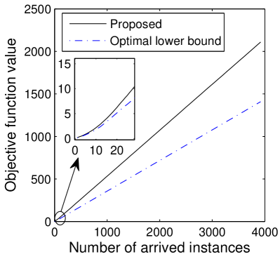
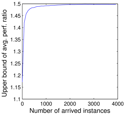
Figure 5: Results with synthetic traces: (a) objective function value, (b) average performance ratio.

6.2 Real-World Traces

To further evaluate the performance while considering the impact of prediction errors and look-ahead window size, we perform simulations using real-world San Francisco taxi traces obtained on the day of May 31, 2008 [31, 32]. Similar to [12], we assume that the MMCs are deployed according to a hexagonal cellular structure in the central area of San Francisco (the center of this area has latitude $37.762$ and longitude $-122.43$). The distance between the center points of adjacent cells is $1000\textrm{ m}$. We consider $K-1=91$ cells (thus MMCs), one backend cloud, and $50$ users (taxis) in total and not all the users are active at a given time. A user is considered active if its most recent location update was received within $600$ s from the current time and its location is within the area covered by MMCs. Each user may require at most one service at a time from the cloud when it is active, where the duration that each active user requires (or, does not require) service is exponentially distributed with a mean value of $50$ slots (or, $10$ slots). When a user requires service, we assume that there is a service instance for this particular request (independent from other users) running on one of the clouds. The local and migration (if migration occurs) resource consumptions of each such instance are set to $1$. We assume that the online algorithm has no knowledge on the departure time of instances and set $T_{\textrm{life}}=\infty$ for all instances. Note that the taxi locations in the dataset are unevenly distributed, so it is still possible that one MMC hosts multiple services although the maximum possible number of instances ($50$) is smaller than the number of MMCs ($91$). The distance metric (for evaluating $r_{k}(t)$ and $s_{kl}(t)$) is defined as the minimum number of hops between two locations on the cellular structure. The physical time corresponding to each slot is set to $60$ s. We set the parameters $\Gamma=1.5,\sigma=2,Y=5,\tilde{g}=\tilde{h}=3,g=h=0.2$. The cost prediction error is assumed to have an upper bound in the form of $F(T)=\beta T^{\alpha}$ (see Section 5.3), where we fix $\alpha=1.1$. The prediction error is generated randomly while ensuring that the upper bound is satisfied.

The simulation results are shown in Fig. 6. In Fig. 6(a), we can see that the result of the proposed online placement approach (E) performs close to the case of online placement with precise future knowledge (D), where approach D assumes that all the future costs as well as instance arrival and departure times are precisely known, but we still use the online algorithm to determine the placement (i.e., we greedily place each instance), because the offline algorithm is too time consuming due to its high complexity. The proposed method E also outperforms alternative methods including only placing on MMCs and never migrate the service instance after initialization (A), always following the user when the user moves to a different cell (B), as well as always placing the service instance on the backend cloud (C). In approaches A and B, the instance placement is determined greedily so that the distance between the instance and its corresponding user is the shortest, subject to the MMC capacity constraint $Y$ so that the costs are finite (see (24)). The fluctuation of the cost during the day is because of different number of users that require the service (thus different system load). In Fig. 6(b), we show the average cost over the day with different look-ahead window sizes and $\beta$ values (a large $\beta$ indicates a large prediction error), where the average results from $8$ different random seeds are shown. We see that the optimal window size ($T^{*}$) found from the method proposed in Section 5 is close to the window size that brings the lowest cost, which implies that the proposed method for finding $T^{*}$ is reasonably accurate.

Additional results on the amount of computation time and floating-point operations (FLOP) for the results in Fig. 6(a) are given in Appendix G.

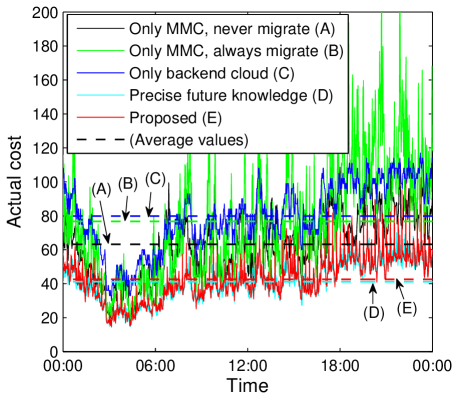
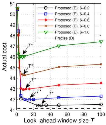
Figure 6: Results with real-world traces (where the costs are summed over all clouds, i.e., the $A(t)$ values): (a) Actual costs at different time of a day, where $\beta=0.4$ for the proposed method E. The arrows point to the average values over the whole day of the corresponding policy. (b) Actual costs averaged over the whole day.

7 Conclusions

In this paper, we have studied the dynamic service placement problem for MMCs with multiple service instances, where the future costs are predictable within a known accuracy. We have proposed algorithms for both offline and online placements, as well as a method for finding the optimal look-ahead window size. The performance of the proposed algorithms has been evaluated both analytically and using simulations with synthetic instance arrival/departure traces and real-world user mobility traces of San Francisco taxis. The simulation results support our analysis.

Our results are based on a general cost function that can represent different aspects in practice. As long as one can assign a cost for every possible configuration, the proposed algorithms are applicable, and the time-complexity results hold. The optimality gap for the online algorithm has been analyzed for a narrower class of functions, which is still very general as discussed earlier in the paper.

The theoretical framework used for analyzing the performance of online placement can be extended to incorporate more general cases, such as those where there exist multiple types of resources in each cloud. We envision that the performance results are similar. We also note that our framework can be applied to analyzing a large class of online resource allocation problems that have convex objective functions.

Shiqiang Wang received the PhD degree from Imperial College London, United Kingdom, in 2015. Before that, he received the MEng and BEng degrees from Northeastern University, China, respectively in 2011 and 2009. He is currently a Research Staff Member at IBM T.J. Watson Research Center, United States, where he also worked as a Graduate-Level Co-op in the summers of 2014 and 2013. In the autumn of 2012, he worked at NEC Laboratories Europe, Germany. His research interests include dynamic control mechanisms, optimization algorithms, protocol design and prototyping, with applications to mobile cloud computing, hybrid and heterogeneous networks, ad-hoc networks, and cooperative communications. He has over 30 scholarly publications, and has served as a technical program committee (TPC) member or reviewer for a number of international journals and conferences. He received the 2015 Chatschik Bisdikian Best Student Paper Award of the Network and Information Sciences International Technology Alliance (ITA).

Rahul Urgaonkar is an Operations Research Scientist with the Modeling and Optimization group at Amazon. Previously, he was with IBM Research where he was a task leader on the US Army Research Laboratory (ARL) funded Network Science Collaborative Technology Alliance (NS CTA) program. He was also a Primary Researcher in the US/UK International Technology Alliance (ITA) research programs. His research is in the area of stochastic optimization, algorithm design and control with applications to communication networks and cloud-computing systems. Dr. Urgaonkar obtained his Masters and PhD degrees from the University of Southern California and his Bachelors degree (all in Electrical Engineering) from the Indian Institute of Technology Bombay.

Ting He received the B.S. degree in computer science from Peking University, China, in 2003 and the Ph.D. degree in electrical and computer engineering from Cornell University, Ithaca, NY, in 2007. She is an Associate Professor in the School of Electrical Engineering and Computer Science at Pennsylvania State University, University Park, PA. From 2007 to 2016, she was a Research Staff Member in the Network Analytics Research Group at IBM T.J. Watson Research Center, Yorktown Heights, NY. Her work is in the broad areas of network modeling and optimization, statistical inference, and information theory. Dr. He is a senior member of IEEE. She has served as the Membership co-chair of ACM N2Women and the GHC PhD Forum committee. She has served on the TPC of a range of communications and networking conferences, including IEEE INFOCOM (Distinguished TPC Member), IEEE SECON, IEEE WiOpt, IEEE/ACM IWQoS, IEEE MILCOM, IEEE ICNC, IFIP Networking, etc. She received the Research Division Award and the Outstanding Contributor Awards from IBM in 2016, 2013, and 2009. She received the Most Collaboratively Complete Publications Award by ITA in 2015, the Best Paper Award at the 2013 International Conference on Distributed Computing Systems (ICDCS), a Best Paper Nomination at the 2013 Internet Measurement Conference (IMC), and the Best Student Paper Award at the 2005 International Conference on Acoustic, Speech and Signal Processing (ICASSP). Her students received the Outstanding Student Paper Award at the 2015 ACM SIGMETRICS and the Best Student Paper Award at the 2013 ITA Annual Fall Meeting.

Kevin Chan is research scientist with the Computational and Information Sciences Directorate at the U.S. Army Research Laboratory (Adelphi, MD). Previously, he was an ORAU postdoctoral research fellow at ARL. His research interests are in network science and dynamic distributed computing, with past work in dynamic networks, trust and distributed decision making and quality of information. He has been an active researcher in ARL’s collaborative programs, the Network Science Collaborative Technology Alliance and Network and Information Sciences International Technology Alliance. Prior to ARL, he received a PhD in Electrical and Computer Engineering (ECE) and MSECE from Georgia Institute of Technology (Atlanta, GA. He also received a BS in ECE/EPP from Carnegie Mellon University (Pittsburgh, PA).

Murtaza Zafer received the B.Tech. degree in Electrical Engineering from the Indian Institute of Technology, Madras, in 2001, and the Ph.D. and S.M. degrees in Electrical Engineering and Computer Science from the Massachusetts Institute of Technology in 2003 and 2007 respectively. He currently works at Nyansa Inc., where he heads the analytics portfolio of the company, building a scalable big data system for analyzing network data. Prior to this, he was a Senior Research Engineer at Samsung Research America, where his research focused on machine learning, deep-neural networks, big data and cloud computing systems. From 2007-2013 he was a Research Scientist at the IBM T.J. Watson Research Center, New York, where his research focused on computer and communication networks, data-analytics and cloud computing. He was a technical lead on several research projects in the US-UK funded multi-institutional International Technology Alliance program with emphasis on fundamental research in mobile wireless networks. He has previously worked at the Corporate R&D center of Qualcomm Inc. and at Bell Laboratories, Alcatel-Lucent Inc., during the summers of 2003 and 2004 respectively. Dr. Zafer serves as an Associate Editor for the IEEE Network magazine. He is a co-recipient of the Best Paper Award at the IEEE/IFIP International Symposium on Integrated Network Management, 2013, and the Best Student Paper award at the International Symposium on Modeling and Optimization in Mobile, Ad Hoc, and Wireless Networks (WiOpt) in 2005, a recipient of the Siemens and Philips Award in 2001 and a recipient of several invention achievement awards at IBM Research.

Kin K. Leung received his B.S. degree from the Chinese University of Hong Kong in 1980, and his M.S. and Ph.D. degrees from University of California, Los Angeles, in 1982 and 1985, respectively. He joined AT&T Bell Labs in New Jersey in 1986 and worked at its successors, AT&T Labs and Lucent Technologies Bell Labs, until 2004. Since then, he has been the Tanaka Chair Professor in the Electrical and Electronic Engineering (EEE), and Computing Departments at Imperial College in London. He is the Head of Communications and Signal Processing Group in the EEE Department. His current research focuses on protocols, optimization and modeling of various wireless networks. He also works on multi-antenna and cross-layer designs for these networks. He received the Distinguished Member of Technical Staff Award from AT&T Bell Labs (1994), and was a co-recipient of the Lanchester Prize Honorable Mention Award (1997). He was elected an IEEE Fellow (2001), received the Royal Society Wolfson Research Merits Award (2004-09) and became a member of Academia Europaea (2012). He also received several best paper awards, including the IEEE PIMRC 2012 and ICDCS 2013. He has actively served on conference committees. He serves as a member (2009-11) and the chairman (2012-15) of the IEEE Fellow Evaluation Committee for Communications Society. He was a guest editor for the IEEE JSAC, IEEE Wireless Communications and the MONET journal, and as an editor for the JSAC: Wireless Series, IEEE Transactions on Wireless Communications and IEEE Transactions on Communications. Currently, he is an editor for the ACM Computing Survey and International Journal on Sensor Networks.

Appendix A Summary of Notations

The main notations used in this paper are summarized in Table I.

Table I: Summary of main notations

Notation	Description
$\triangleq$	Defined to be equal to
$\cdot$	Dot-product
$K$	Total number of clouds
$k,l\in\{1,2,...,K\}$	Cloud index
$t$	Timeslot index
$T$	Size of look-ahead window
$M$	Total/maximum number of service instances under consideration
$i$	Service instance index
$\bm{\pi}(t_{0},...,t_{n})$	Configuration matrix for slots $\{t_{0},...,t_{n}\}$, written in $\bm{\pi}$ for short
$U(t,\bm{\pi}(t))$	Local cost in slot $t$
$W(t,\bm{\pi}(t-1),\bm{\pi}(t))$	Migration cost between slots $t-1$ and $t$
$C_{\bm{\pi}(t-1,t)}(t)$	Sum of local and migration costs in slot $t$ when following configuration $\bm{\pi}(t-1,t)$
$A_{\bm{\pi}(t-1,t)}(t)$	Actual cost (actual value of $C_{\bm{\pi}(t-1,t)}(t)$)
$D_{\bm{\pi}(t-1,t)}^{t_{0}}(t)$	Predicted cost (predicted value of $C_{\bm{\pi}(t-1,t)}(t)$ when prediction is made at slot $t_{0}$)
$\epsilon(\tau)$	Equal to $\max_{\bm{\pi}(t-1,t),t_{0}}\left|A_{\bm{\pi}(t-1,t)}(t_{0}+\tau)-D_{\bm{\pi}(t-1,t)}^{t_{0}}(t_{0}+\tau)\right|$, the maximum error when looking ahead for $\tau$ slots
$\Lambda$	Set of all possible configuration sequences
$\bm{\lambda}\in\Lambda$	Configuration sequence (when considering a particular instance $i$, it is equal to the $i$th column of $\bm{\pi}$)
$\Lambda_{i}\subseteq\Lambda$	Subset of configuration sequences that conform to the arrival and departure times of instance $i$
$x_{i\bm{\lambda}}$	Binary variable specifying whether instance $i$ operates in configuration sequence $\bm{\lambda}$
$a_{i\bm{\lambda}k}(t)$	Local resource consumption at cloud $k$ in slot $t$ when instance $i$ is operating under configuration sequence $\bm{\lambda}$
$b_{i\bm{\lambda}kl}(t)$	Migration resource consumption when instance $i$ operating under configuration sequence $\bm{\lambda}$ is assigned to cloud $k$ in slot $t-1$ and to cloud $l$ in slot $t$
$y_{k}(t)$	Equal to $\sum_{i=1}^{M}\sum_{\bm{\lambda}\in\Lambda}a_{i\bm{\lambda}k}(t)x_{i\bm{\lambda}}$, sum local resource consumption at cloud $k$
$z_{kl}(t)$	Equal to $\sum_{i=1}^{M}\sum_{\bm{\lambda}\in\Lambda}b_{i\bm{\lambda}kl}(t)x_{i\bm{\lambda}}$, sum migration resource consumption from cloud $k$ to cloud $l$
$u_{k,t}\left(y_{k}(t)\right)$	Local cost at cloud $k$ in timeslot $t$
$w_{kl,t}\left(y_{k}(t-1),y_{l}(t),z_{kl}(t)\right)$	Migration cost from cloud $k$ to cloud $l$ between slots $t-1$ and $t$
$\left(\mathbf{g}\right)_{h_{1}h_{2}}$ (or $\left(\mathbf{g}\right)_{h_{1}h_{2}h_{3}}$)	The $(h_{1},h_{2})$th (or $(h_{1},h_{2},h_{3})$th) element in an arbitrary vector or matrix $\mathbf{g}$
$\mathbf{y}$	Vector with elements $\left(\mathbf{y}\right)_{kt}\triangleq y_{k}(t)$
$\mathbf{z}$	Vector with elements $\left(\mathbf{z}\right)_{klt}\triangleq z_{kl}(t)$
$\mathbf{x}$	Vector with elements $\left(\mathbf{x}\right)_{i\bm{\lambda}}\triangleq x_{i\bm{\lambda}}$
$\mathbf{a}_{i\bm{\lambda}}$	Vector with elements $\left(\mathbf{a}_{i\bm{\lambda}}\right)_{kt}\triangleq a_{i\bm{\lambda}k}(t)$
$\mathbf{b}_{i\bm{\lambda}}$	Vector with elements $\left(\mathbf{b}_{i\bm{\lambda}}\right)_{klt}\triangleq b_{i\bm{\lambda}kl}(t)$
$\widetilde{D}\left(\mathbf{x}\right)$, $\widetilde{D}\left(\mathbf{y},\mathbf{z}\right)$	Sum (predicted) cost of all $T$ slots, defined in (7)
$\phi$, $\psi$	Parameters related to the performance gap, defined in (11) and (12)
$\Gamma$	Competitive ratio of Algorithm 3
$\sigma$	Parameter related to the migration cost, defined in (17)
$F(T)$	Equal to $\sum_{t=t_{0}}^{t_{0}+T-1}\epsilon(t-t_{0})$, the sum-error starting from slot $t_{0}$ up to slot $t_{0}+T-1$
$G(T)$	The continuous time extension of $F(T)$, see Section 5.2
$\theta(T)$	Equal to $\frac{(\Gamma+1)G(T)+\sigma}{T}$, the upper bound in (19) after replacing $F(T)$ with $G(T)$

Note: The timeslot argument $t$ may be omitted in some parts of the discussion for simplicity. Vector elements are referred to with multiple indexes, but we regard vectors as single-indexed vectors for the purposes of vector concatenation (i.e., joining two vectors into one vector) and gradient computation.

Appendix B Proof of Proposition 1

We show that problem (8) can be reduced from the partition problem, which is known to be NP-complete [29, Corollary 15.28]. The partition problem is defined as follows.

Definition 1.

(Partition Problem) Given positive integers $v_{1},v_{2},...,v_{M}$, is there a subset $\mathcal{S}\subseteq\{1,2,...,M\}$ such that $\sum_{j\in\mathcal{S}}v_{j}=\sum_{j\in\mathcal{S}^{c}}v_{j}$, where $\mathcal{S}^{c}$ is the complement set of $\mathcal{S}$?

Similarly to the proof of [29, Theorem 18.1], we define a decision version of the bin packing problem, where we assume that there are $M$ items each with size

$$a_{i}\triangleq\frac{2v_{i}}{\sum_{j=1}^{M}v_{j}}$$

for all $i\in\{1,2,...,M\}$, and the problem is to determine whether these $M$ items can be packed into two bins each with unit size (i.e., its size is equal to one). It is obvious that this bin packing decision problem is equivalent to the partition problem.

To solve the above defined bin packing decision problem, we can set $t_{0}=1$, $T=1$, and $K=2$ in (8). Because we attempt to place all items, we set $\Lambda_{i}=\{1,2\}$ for all $i$. By definition, $w_{kl,t}(\cdot,\cdot,\cdot)=0$ for $t=1$. We omit the subscript $t$ in the following as we only consider a single slot. We define $a_{i\bm{\lambda}k}=a_{i}$ for all $\bm{\lambda},k$, and define

$$u_{k}(y)=\begin{cases}\epsilon y,&\textrm{if }y\leq 1\\ \frac{2\epsilon}{c}(y-1)+\epsilon,&\textrm{if }y>1\end{cases}$$ (27)

where $c\triangleq\frac{1}{\sum_{j=1}^{M}v_{j}}$, and $\epsilon>0$ is an arbitrary constant.

Because $v_{i}$ is a positive integer for any $i$, we have that $\frac{a_{i}}{c}=2v_{i}$ is always a positive integer, and $\frac{1}{c}=\sum_{j=1}^{M}v_{j}$ is also always a positive integer. It follows that $y$ can only be integer multiples of $c$ (where we recall that $y$ is the sum of $a_{i}$ for those items $i$ that are placed in the bin), and there exists a positive integer $c^{\prime}\triangleq\sum_{j=1}^{M}v_{j}$ such that $c^{\prime}c=1$. Thus, when $y>1$, we always have $y-1\geq c$. Therefore, the choice of $u_{k}(y)$ in (27) guarantees that $u_{k}(y_{k})\geq 3\epsilon>2\epsilon$ whenever bin $k$ ($k\in\{1,2\}$) exceeds its size, and $\sum_{k=1}^{2}u_{k}\left(y_{k}\right)\leq 2\epsilon$ when no bin has exceeded its size. At the same time, $u_{k}(y)$ satisfies Assumption 1 as long as $c\leq 2$.

By the definition of $c$, we always have $c\leq 2$ because $\sum_{j=1}^{M}v_{j}\geq 1$. To solve the bin packing decision problem defined above (thus the partition problem), we can solve (8) with the above definitions. If the solution is not larger than $2\epsilon$, the packing is feasible and the answer to the partition problem is “yes”; otherwise, the packing is infeasible and the answer to the partition problem is “no”. It follows that problem (8) is “at least as hard as” the partition problem, which proves that (8) is NP-hard.

Appendix C Proof of Proposition 2

We first introduce a few lemmas, with results used later in the proof.

Lemma 2.

For any instance $j$ and configuration sequence $\bm{\lambda}$, we have

$$\frac{\partial\widetilde{D}}{\partial x_{j\bm{\lambda}}}\left(\mathbf{x}\right)=\nabla_{\mathbf{y,z}}\widetilde{D}\left(\mathbf{y},\mathbf{z}\right)\cdot\left(\mathbf{a}_{j\bm{\lambda}},\mathbf{b}_{j\bm{\lambda}}\right)$$ (28)

Proof.

$$\frac{\partial\widetilde{D}}{\partial x_{j\bm{\lambda}}}\left(\mathbf{x}\right) =\!\!\!\sum_{t=t_{0}}^{t_{0}+T-1}\Bigg{[}\sum_{k=1}^{K}\frac{\partial\widetilde{D}}{\partial y_{k}(t)}\left(\mathbf{x}\right)\cdot\frac{\partial y_{k}(t)}{\partial x_{j\bm{\lambda}}}\left(\mathbf{x}\right)+$$

$$\quad\sum_{k=1}^{K}\sum_{l=1}^{K}\frac{\partial\widetilde{D}}{\partial z_{kl}(t)}\left(\mathbf{x}\right)\cdot\frac{\partial z_{kl}(t)}{\partial x_{j\bm{\lambda}}}\left(\mathbf{x}\right)\Bigg{]}$$

$$=\!\!\!\sum_{t=t_{0}}^{t_{0}+T-1}\Bigg{[}\sum_{k=1}^{K}\frac{\partial\widetilde{D}}{\partial y_{k}(t)}\left(\mathbf{x}\right)\cdot a_{j\bm{\lambda}k}(t)+$$

$$\quad\sum_{k=1}^{K}\sum_{l=1}^{K}\frac{\partial\widetilde{D}}{\partial z_{kl}(t)}\left(\mathbf{x}\right)\cdot b_{j\bm{\lambda}kl}(t)\Bigg{]}$$

$$=\nabla_{\mathbf{y,z}}\widetilde{D}\left(\mathbf{y},\mathbf{z}\right)\cdot\left(\mathbf{a}_{j\bm{\lambda}},\mathbf{b}_{j\bm{\lambda}}\right)$$

where we recall that $y_{k}(t)$ and $z_{kl}(t)$ are functions of $x_{j\bm{\lambda}}$ for all $j$ and $\bm{\lambda}$, thus they are also functions of vector $\mathbf{x}$. ∎

Lemma 3.

For any instance $j$ and configuration sequence $\bm{\lambda}$, we have

$$\nabla_{\mathbf{x}}\widetilde{D}\left(\mathbf{x}\right)\cdot\mathbf{x}=\nabla_{\mathbf{y,z}}\widetilde{D}\left(\mathbf{y},\mathbf{z}\right)\cdot\left(\mathbf{y},\mathbf{z}\right)$$ (29)

Proof.

$$\nabla_{\mathbf{x}}\widetilde{D}\left(\mathbf{x}\right)\cdot\mathbf{x}$$

$$=\sum_{j=1}^{M}\sum_{\bm{\lambda}\in\Lambda}\frac{\partial\widetilde{D}}{\partial x_{j\bm{\lambda}}}\left(\mathbf{x}\right)\cdot x_{j\bm{\lambda}}$$

$$=\sum_{j=1}^{M}\sum_{\bm{\lambda}\in\Lambda}\nabla_{\mathbf{y,z}}\widetilde{D}\left(\mathbf{y},\mathbf{z}\right)\cdot\left(\mathbf{a}_{j\bm{\lambda}},\mathbf{b}_{j\bm{\lambda}}\right)\cdot x_{j\bm{\lambda}}$$

$$=\nabla_{\mathbf{y,z}}\widetilde{D}\left(\mathbf{y},\mathbf{z}\right)\cdot\left(\sum_{j=1}^{M}\sum_{\bm{\lambda}\in\Lambda}\left(\mathbf{a}_{j\bm{\lambda}},\mathbf{b}_{j\bm{\lambda}}\right)\cdot x_{j\bm{\lambda}}\right)$$

$$=\nabla_{\mathbf{y,z}}\widetilde{D}\left(\mathbf{y},\mathbf{z}\right)\cdot\left(\mathbf{y},\mathbf{z}\right)$$

where the second step follows from Lemma 2, the last step follows from the definition of vectors $\mathbf{y},\mathbf{z},\mathbf{a}_{j\bm{\lambda}},\mathbf{b}_{j\bm{\lambda}}$. ∎

We introduce some additional notations that are used in the proof below. Recall that the values of vectors $\mathbf{x}$, $\mathbf{y}$, and $\mathbf{z}$ may vary over time due to service arrivals and departures. Let $\mathbf{x}_{j}^{(j)}$, $\mathbf{y}_{j}^{(j)}$, and $\mathbf{z}_{j}^{(j)}$ respectively denote the values of $\mathbf{x}$, $\mathbf{y}$, and $\mathbf{z}$ immediately after instance $j$ is placed; and let $\mathbf{x}_{j-1}^{(j)}$, $\mathbf{y}_{j-1}^{(j)}$, and $\mathbf{z}_{j-1}^{(j)}$ respectively denote the values of $\mathbf{x}$, $\mathbf{y}$, and $\mathbf{z}$ immediately before instance $j$ is placed. We note that the values of $\mathbf{x}$, $\mathbf{y}$, and $\mathbf{z}$ may change after placing each instance. Therefore, the notions of “before”, “after”, and “time” (used below) here correspond to the sequence of service instance placement, instead of the actual physical time.

We then introduce vectors that only consider the placement up to the $j$th service instance, which are necessary because the proof below uses an iterative approach. Let $\mathbf{x}_{j}$, $\mathbf{y}_{j}$, and $\mathbf{z}_{j}$ respectively denote the values of $\mathbf{x}$, $\mathbf{y}$, and $\mathbf{z}$ at any time after placing instance $j$ (where instance $j$ can be either still running in the system or already departed) while ignoring the placement of any subsequent instances $j^{\prime}>j$ (if any). This means, in vector $\mathbf{x}_{j}$, we set $\left(\mathbf{x}_{j}\right)_{i\bm{\lambda}}\triangleq x_{i\bm{\lambda}}$ for any $i\leq j$ and $\bm{\lambda}$, and set $\left(\mathbf{x}_{j}\right)_{i\bm{\lambda}}\triangleq 0$ for any $i>j$ and $\bm{\lambda}$, although the value of $x_{i\bm{\lambda}}$ at the current time of interest may be non-zero for some $i>j$ and $\bm{\lambda}$. Similarly, in vectors $\mathbf{y}_{j}$ and $\mathbf{z}_{j}$, we only consider the resource consumptions up to instance $j$, i.e., $\left(\mathbf{y}_{j}\right)_{kt}\triangleq\sum_{i=1}^{j}\sum_{\bm{\lambda}\in\Lambda}a_{i\bm{\lambda}k}(t)x_{i\bm{\lambda}}$ and $\left(\mathbf{z}_{j}\right)_{klt}\triangleq\sum_{i=1}^{j}\sum_{\bm{\lambda}\in\Lambda}b_{i\bm{\lambda}kl}(t)x_{i\bm{\lambda}}$ for any $k$, $l$, and $t$.

We assume that the last service instance that has arrived before the current time of interest has index $M$, thus $\mathbf{x}=\mathbf{x}_{M}$, $\mathbf{y}=\mathbf{y}_{M}$, and $\mathbf{z}=\mathbf{z}_{M}$.

Because an instance will never come back after it has departed (even if an instance of the same type comes back, it will be given a new index), we have $\mathbf{y}{}_{j-1}\leq\mathbf{y}_{j-1}^{(j)}$ and $\mathbf{z}{}_{j-1}\leq\mathbf{z}_{j-1}^{(j)}$, where the inequalities are defined element-wise for the vector.

Define $v_{j}\triangleq\widetilde{D}\left(\mathbf{y}_{j}^{(j)},\mathbf{z}_{j}^{(j)}\right)-\widetilde{D}\left(\mathbf{y}_{j-1}^{(j)},\mathbf{z}_{j-1}^{(j)}\right)$ to denote the increase in the sum cost $\widetilde{D}(\mathbf{y},\mathbf{z})$ (or, equivalently, $\widetilde{D}(\mathbf{x})$) at the time when placing service $j$. Note that after this placement, the value of $\widetilde{D}\left(\mathbf{y}_{j},\mathbf{z}_{j}\right)-\widetilde{D}\left(\mathbf{y}_{j-1},\mathbf{z}_{j-1}\right)$ may vary over time, because some services $i\leq j$ may leave the system, but the value of $v_{j}$ is only taken when service $j$ is placed upon its arrival.

Lemma 4.

When Assumption 1 is satisfied, for any $M$, we have

$$\widetilde{D}\left(\mathbf{x}_{M}\right)\leq\sum_{j=1}^{M}v_{j}$$ (30)

Proof.

Assume that service $j$ takes configuration $\bm{\lambda}_{0}$ after its placement (and before it possibly unpredictably departs), then $\mathbf{y}_{j}^{(j)}-\mathbf{y}_{j-1}^{(j)}=\mathbf{a}{}_{j\bm{\lambda}_{0}}$ and $\mathbf{z}_{j}^{(j)}-\mathbf{z}_{j-1}^{(j)}=\mathbf{b}{}_{j\bm{\lambda}_{0}}$. For any time after placing instance $j$ we define $\Delta\mathbf{y}_{j}\triangleq\mathbf{y}{}_{j}-\mathbf{y}{}_{j-1}$ and $\Delta\mathbf{z}_{j}\triangleq\mathbf{z}{}_{j}-\mathbf{z}{}_{j-1}$. We always have $\Delta\mathbf{y}_{j}=\mathbf{a}{}_{j\bm{\lambda}_{0}}$, $\Delta\mathbf{z}_{j}=\mathbf{b}{}_{j\bm{\lambda}_{0}}$, if instance $j$ has not yet departed from the system, and $\Delta\mathbf{y}_{j}=\Delta\mathbf{z}_{j}=0$ if $j$ has already departed from the system.

Noting that $\widetilde{D}\left(\mathbf{y}_{j},\mathbf{z}_{j}\right)$ is convex non-decreasing (from Lemma 1), we have

$$\widetilde{D}\left(\mathbf{y}{}_{j},\mathbf{z}{}_{j}\right)-\widetilde{D}\left(\mathbf{y}{}_{j-1},\mathbf{z}{}_{j-1}\right)$$

$$=\widetilde{D}\left(\mathbf{y}{}_{j-1}+\Delta\mathbf{y}_{j},\mathbf{z}{}_{j-1}+\Delta\mathbf{z}_{j}\right)-\widetilde{D}\left(\mathbf{y}{}_{j-1},\mathbf{z}{}_{j-1}\right)$$

$$\leq\widetilde{D}\left(\mathbf{y}{}_{j-1}^{(j)}+\Delta\mathbf{y}_{j},\mathbf{z}{}_{j-1}^{(j)}+\Delta\mathbf{z}_{j}\right)-\widetilde{D}\left(\mathbf{y}{}_{j-1}^{(j)},\mathbf{z}{}_{j-1}^{(j)}\right)$$ (31)

$$\leq\widetilde{D}\left(\mathbf{y}{}_{j-1}^{(j)}+\mathbf{a}{}_{j\bm{\lambda}_{0}},\mathbf{z}{}_{j-1}^{(j)}+\mathbf{b}{}_{j\bm{\lambda}_{0}}\right)-\widetilde{D}\left(\mathbf{y}{}_{j-1}^{0},\mathbf{z}{}_{j-1}^{0}\right)$$ (32)

$$=\widetilde{D}\left(\mathbf{y}_{j}^{(j)},\mathbf{z}_{j}^{(j)}\right)-\widetilde{D}\left(\mathbf{y}_{j-1}^{(j)},\mathbf{z}_{j-1}^{(j)}\right)$$

$$=v_{j}$$

where inequality (31) is because $\mathbf{y}{}_{j-1}\leq\mathbf{y}_{j-1}^{(j)}$, $\mathbf{z}{}_{j-1}\leq\mathbf{z}_{j-1}^{(j)}$ (see discussion above) and due to the convex non-decreasing property of $\widetilde{D}\left(\mathbf{y}_{j},\mathbf{z}_{j}\right)$; inequality (32) is because $\Delta\mathbf{y}_{j}\leq\mathbf{a}{}_{j\bm{\lambda}_{0}}$, $\Delta\mathbf{z}_{j}\leq\mathbf{b}{}_{j\bm{\lambda}_{0}}$ and also due to the non-decreasing property of $\widetilde{D}\left(\mathbf{y}_{j},\mathbf{z}_{j}\right)$.

We now note that $\widetilde{D}\left(\mathbf{x}_{0}\right)=0$, where $\mathbf{x}_{0}=\mathbf{0}$ and $\mathbf{0}$ is defined as a vector with all zeros, thus $\mathbf{y}_{0}=\mathbf{z}_{0}=\mathbf{0}$. We have

$$\sum_{j=1}^{M}v_{j} \geq\sum_{j=1}^{M}\left[\widetilde{D}\left(\mathbf{y}{}_{j},\mathbf{z}{}_{j}\right)-\widetilde{D}\left(\mathbf{y}{}_{j-1},\mathbf{z}{}_{j-1}\right)\right]$$

$$=\widetilde{D}\left(\mathbf{x}_{M}\right)-\widetilde{D}\left(\mathbf{x}_{0}\right)=\widetilde{D}\left(\mathbf{x}_{M}\right)$$

∎

Lemma 5.

When Assumption 1 is satisfied, for any $j$ and $\bm{\lambda}$, we have

$$v_{j}\leq\phi\frac{\partial\widetilde{D}}{\partial x_{j\bm{\lambda}}}\left(\mathbf{x}_{M}\right)$$ (33)

where $\phi$ is a constant satisfying (11).

Proof.

Assume that service $j$ takes configuration $\bm{\lambda}_{0}$ after its placement (and before it possibly unpredictably departs). Because we perform a greedy assignment in Algorithm 3, we have

$$v_{j} =\widetilde{D}\left(\mathbf{y}_{j}^{(j)},\mathbf{z}_{j}^{(j)}\right)-\widetilde{D}\left(\mathbf{y}_{j-1}^{(j)},\mathbf{z}_{j-1}^{(j)}\right)$$

$$=\widetilde{D}\left(\mathbf{y}_{j-1}^{(j)}+\mathbf{a}_{j\bm{\lambda}_{0}},\mathbf{z}_{j-1}^{(j)}+\mathbf{b}_{j\bm{\lambda}_{0}}\right)-\widetilde{D}\left(\mathbf{y}_{j-1}^{(j)},\mathbf{z}_{j-1}^{(j)}\right)$$

$$\leq\widetilde{D}\left(\mathbf{y}_{j-1}^{(j)}+\mathbf{a}_{j\bm{\lambda}},\mathbf{z}_{j-1}^{(j)}+\mathbf{b}_{j\bm{\lambda}}\right)-\widetilde{D}\left(\mathbf{y}_{j-1}^{(j)},\mathbf{z}_{j-1}^{(j)}\right)$$

for any $\bm{\lambda}\in\Lambda_{i}$.

Then, we have

$$\widetilde{D}\left(\mathbf{y}_{j-1}^{(j)}+\mathbf{a}_{j\bm{\lambda}},\mathbf{z}_{j-1}^{(j)}+\mathbf{b}_{j\bm{\lambda}}\right)-\widetilde{D}\left(\mathbf{y}_{j-1}^{(j)},\mathbf{z}_{j-1}^{(j)}\right)$$

$$\leq\nabla_{\mathbf{y,z}}\widetilde{D}\left(\mathbf{y}_{j-1}^{(j)}+\mathbf{a}_{j\bm{\lambda}},\mathbf{z}_{j-1}^{(j)}+\mathbf{b}_{j\bm{\lambda}}\right)\cdot\left(\mathbf{a}_{j\bm{\lambda}},\mathbf{b}_{j\bm{\lambda}}\right)$$ (34)

$$\leq\nabla_{\mathbf{y,z}}\widetilde{D}\left(\mathbf{y}_{\textrm{max}}+\mathbf{a}_{j\bm{\lambda}},\mathbf{z}_{\textrm{max}}+\mathbf{b}_{j\bm{\lambda}}\right)\cdot\left(\mathbf{a}_{j\lambda},\mathbf{b}_{j\bm{\lambda}}\right)$$ (35)

$$\leq\phi\nabla_{\mathbf{y,z}}\widetilde{D}\left(\mathbf{y}_{M},\mathbf{z}_{M}\right)\cdot\left(\mathbf{a}_{j\bm{\lambda}},\mathbf{b}_{j\bm{\lambda}}\right)$$ (36)

$$=\phi\frac{\partial\widetilde{D}}{\partial x_{j\bm{\lambda}}}\left(\mathbf{x}_{M}\right)$$ (37)

where “$\cdot$” denotes the dot-product. The above relationship is explained as follows. Inequality (34) follows from the first-order conditions of convex functions [30, Section 3.1.3]. The definition of $\mathbf{y}_{\textrm{max}}$ and $\mathbf{z}_{\textrm{max}}$ in Proposition 2 gives (35). The definition of $\phi$ in (11) gives (36). Equality (37) follows from Lemma 2. This completes the proof. ∎

Using the above lemmas, we now proof Proposition 2.

Proof.

(Proposition 2) Due to the convexity of $\widetilde{D}(\mathbf{x})$, from the first-order conditions of convex functions [30, Section 3.1.3], we have

$$\widetilde{D}(\phi\psi\mathbf{x}_{M}^{*})-\widetilde{D}(\mathbf{x}_{M})$$

$$\geq\nabla_{\mathbf{x}}\widetilde{D}\left(\mathbf{x}_{M}\right)\cdot\left(\phi\psi\mathbf{x}_{M}^{*}-\mathbf{x}_{M}\right)$$ (38)

$$=\phi\psi\nabla_{\mathbf{x}}\widetilde{D}\left(\mathbf{x}_{M}\right)\cdot\mathbf{x}_{M}^{*}-\nabla_{\mathbf{x}}\widetilde{D}\left(\mathbf{x}_{M}\right)\mathbf{x}_{M}$$ (39)

$$=\sum_{i=1}^{M}\sum_{\bm{\lambda}\in\Lambda}\phi\psi x_{i\bm{\lambda}}^{*}\frac{\partial\widetilde{D}}{\partial x_{i\bm{\lambda}}}\left(\mathbf{x}_{M}\right)-\nabla_{\mathbf{x}}\widetilde{D}\left(\mathbf{x}_{M}\right)\cdot\mathbf{x}_{M}$$ (40)

$$=\psi\left(\sum_{i=1}^{M}\sum_{\bm{\lambda}\in\Lambda}x_{i\bm{\lambda}}^{*}\phi\frac{\partial\widetilde{D}}{\partial x_{i\bm{\lambda}}}\left(\mathbf{x}_{M}\right)-\frac{\nabla_{\mathbf{x}}\widetilde{D}\left(\mathbf{x}_{M}\right)\cdot\mathbf{x}_{M}}{\psi}\right)$$ (41)

where $x_{i\bm{\lambda}}^{*}$ is the $(i,\bm{\lambda})$th element of vector $\mathbf{x}_{M}^{*}$. From Lemma 5, we have

Eq. (41) $$\geq\psi\left(\sum_{i=1}^{M}\sum_{\bm{\lambda}\in\Lambda}x_{i\bm{\lambda}}^{*}v_{i}-\frac{\nabla_{\mathbf{x}}\widetilde{D}\left(\mathbf{x}_{M}\right)\cdot\mathbf{x}_{M}}{\psi}\right)$$ (42)

$$=\psi\left(\sum_{i=1}^{M}v_{i}\sum_{\bm{\lambda}\in\Lambda}x_{i\bm{\lambda}}^{*}-\frac{\nabla_{\mathbf{x}}\widetilde{D}\left(\mathbf{x}_{M}\right)\cdot\mathbf{x}_{M}}{\psi}\right)$$ (43)

From the constraint $\sum_{\bm{\lambda}\in\Lambda}x_{i\bm{\lambda}}^{*}=1$ and the definition of $\psi$, we get

Eq. (43) $$=\psi\left(\sum_{i=1}^{M}v_{i}-\frac{\nabla_{\mathbf{x}}\widetilde{D}\left(\mathbf{x}_{M}\right)\cdot\mathbf{x}_{M}}{\psi}\right)$$ (44)

$$\geq\psi\left(\sum_{i=1}^{M}v_{i}-\widetilde{D}(\mathbf{x}_{M})\right)$$ (45)

$$\geq 0$$ (46)

where the last equality follows from Lemma 4. This gives (9).

Equation (10) follows from the fact that $y_{k,j}(t)$ and $z_{kl,j}(t)$ are both linear in $x_{i\lambda}$.

The last equality in (12) follows from Lemma 3 and the fact that $\widetilde{D}\left(\mathbf{x}\right)=\widetilde{D}\left(\mathbf{y},\mathbf{z}\right)$ as well as $\mathbf{x}=\mathbf{x}_{M}$, $\mathbf{y}=\mathbf{y}_{M}$, and $\mathbf{z}=\mathbf{z}_{M}$.∎

Appendix D Proof of Proposition 4

Lemma 6.

For polynomial functions $\Xi_{1}(y)$ and $\Xi_{2}(y)$ in the general form:

$$\Xi_{1}(y) \triangleq\sum_{\rho=0}^{\Omega}\omega_{1}^{(\rho)}y^{\rho}$$

$$\Xi_{2}(y) \triangleq\sum_{\rho=0}^{\Omega}\omega_{2}^{(\rho)}y^{\rho}$$

where the constants $\omega_{1}^{(\rho)}\geq 0$ and $\omega_{2}^{(\rho)}\geq 0$ for $0\leq\rho<\Omega$, while $\omega_{1}^{(\Omega)}>0$ and $\omega_{2}^{(\Omega)}>0$, we have

$$\lim_{y\rightarrow+\infty}\frac{\Xi_{1}(y)}{\Xi_{2}(y)}=\frac{\omega_{1}^{(\Omega)}}{\omega_{2}^{(\Omega)}}$$

Proof.

When $\Omega=0$, we have

$$\lim_{y\rightarrow+\infty}\frac{\Xi_{1}(y)}{\Xi_{2}(y)}=\frac{\omega_{1}^{(0)}}{\omega_{2}^{(0)}}$$

When $\Omega>0$, we note that $\lim_{y\rightarrow+\infty}\Xi_{1}(y)=+\infty$ and $\lim_{y\rightarrow+\infty}\Xi_{2}(y)=+\infty$, because $\omega_{1}^{(\Omega)}>0$ and $\omega_{2}^{(\Omega)}>0$. We apply the L’Hospital’s rule and get

$$\lim_{y\rightarrow+\infty}\frac{\Xi_{1}(y)}{\Xi_{2}(y)} =\lim_{y\rightarrow+\infty}\frac{\frac{d\Xi_{1}(y)}{dy}}{\frac{d\Xi_{2}(y)}{dy}}$$

$$=\lim_{y\rightarrow+\infty}\frac{\sum_{\rho=1}^{\Omega}\rho\omega_{1}^{(\rho)}y^{\rho-1}}{\sum_{\rho=1}^{\Omega}\rho\omega_{2}^{(\rho)}y^{\rho-1}}$$ (47)

Suppose we have

$$\lim_{y\rightarrow+\infty}\frac{\Xi_{1}(y)}{\Xi_{2}(y)} =\lim_{y\rightarrow+\infty}\frac{\sum_{\rho=n}^{\Omega}\left(\prod_{m=0}^{n-1}(\rho-m)\right)\omega_{1}^{(\rho)}y^{\rho-n}}{\sum_{\rho=n}^{\Omega}\left(\prod_{m=0}^{n-1}(\rho-m)\right)\omega_{2}^{(\rho)}y^{\rho-n}}$$ (48)

which equals to (47) for $n=1$. For $1\leq n<\Omega$, we note that $\Omega-n>0$, hence the numerator and denominator in the right hand-side (RHS) of (48) still respectively approach $+\infty$ when $y\rightarrow+\infty$ (because $\omega_{1}^{(\Omega)}>0$ and $\omega_{2}^{(\Omega)}>0$). Let $\Psi(n)$ denote the RHS (48), we can reapply the L’Hospital’s rule on $\Psi(n)$, yielding

$$\Psi(n) =\lim_{y\rightarrow+\infty}\frac{\sum_{\rho=n+1}^{\Omega}\left(\prod_{m=0}^{(n+1)-1}(\rho-m)\right)\omega_{1}^{(\rho)}y^{\rho-(n+1)}}{\sum_{\rho=n+1}^{\Omega}\left(\prod_{m=0}^{(n+1)-1}(\rho-m)\right)\omega_{2}^{(\rho)}y^{\rho-(n+1)}}$$

$$=\Psi(n+1)$$

which proofs that (48) holds for $1\leq n\leq\Omega$. Therefore,

$$\lim_{y\rightarrow+\infty}\frac{\Xi_{1}(y)}{\Xi_{2}(y)} =\Psi(\Omega)=\frac{\rho!\omega_{1}^{(\Omega)}}{\rho!\omega_{2}^{(\Omega)}}=\frac{\omega_{1}^{(\Omega)}}{\omega_{2}^{(\Omega)}}$$

∎

Lemma 7.

For variables $0\leq y\leq y^{\prime},0\leq y_{k}\leq y^{\prime}_{k},0\leq y_{l}\leq y^{\prime}_{l},0\leq z_{kl}\leq z^{\prime}_{kl}$, we always have

$$\frac{du_{k,t}}{dy}(y) \leq\frac{du_{k,t}}{dy}(y^{\prime})$$ (49)

$$\frac{\partial w_{kl,t}}{\partial\Upsilon}(y_{k},y_{l},z_{kl}) \leq\frac{\partial w_{kl,t}}{\partial\Upsilon}(y^{\prime}_{k},y^{\prime}_{l},z^{\prime}_{kl})$$ (50)

where $\Upsilon$ stands for either $y_{k}$, $y_{l}$, or $z_{kl}$.

Proof.

We note that

$$\frac{du_{k,t}}{dy}(y)=\sum_{\rho}\rho\gamma_{k,t}^{(\rho)}y^{\rho-1}$$

from which (49) follows directly because $\gamma_{k,t}^{(\rho)}\geq 0$. We then note that

$$\frac{\partial w_{kl,t}}{\partial y_{k}}(y_{k},y_{l},z_{kl})=\sum_{\rho_{1}}\sum_{\rho_{2}}\sum_{\rho_{3}}\rho_{1}\kappa_{kl,t}^{(\rho_{1},\rho_{2},\rho_{3})}y_{k}^{\rho_{1}-1}y_{l}^{\rho_{2}}z_{kl}^{\rho_{3}}$$

from which (50) follows for $\Upsilon=y_{k}$ because $\kappa_{kl,t}^{(\rho_{1},\rho_{2},\rho_{3})}\geq 0$. Similarly, (50) also follows for $\Upsilon=y_{l}$ and $\Upsilon=z_{kl}$. ∎

Lemma 8.

Let $\Omega$ denote the maximum value of $\rho$ such that either $\gamma_{k,t}^{(\rho)}>0$ or $\kappa_{kl,t}^{(\rho_{1},\rho_{2},\rho_{3})}>0$, where $\rho_{1}+\rho_{2}+\rho_{3}=\rho$. Assume that the cost functions are defined as in (15) and (16), then for any constants $\delta>0$, $B\geq 0$, there exist sufficiently large values of $y,y_{k},y_{l},z_{kl}$, such that

$$\frac{\frac{du_{k,t}}{dy}(y+B)}{\frac{du_{k,t}}{dy}(y)} \leq 1+\delta$$ (51)

$$\frac{\frac{du_{k,t}}{dy}(y)\cdot y}{u_{k,t}(y)} \leq\Omega+\delta$$ (52)

$$\frac{\frac{\partial w_{kl,t}}{\partial\Upsilon}(y_{k}+B,y_{l}+B,z_{kl}+B)}{\frac{\partial w_{kl,t}}{\partial\Upsilon}(y_{k},y_{l},z_{kl})} \leq 1+\delta$$ (53)

$$\frac{\frac{\partial w_{kl,t}}{\partial\Upsilon}(y_{k},y_{l},z_{kl})\cdot\Upsilon}{w_{k,t}(y_{k},y_{l},z_{kl})} \leq\Omega+\delta$$ (54)

for any $k,l,t$, where $\Upsilon$ stands for either $y_{k}$, $y_{l}$, or $z_{kl}$.

Proof.

Let $\Omega^{\prime}$ denote the maximum value of $\rho$ such that $\gamma_{k,t}^{(\rho)}>0$, we always have $\Omega^{\prime}\leq\Omega$. We note that

$$\frac{\frac{du_{k,t}}{dy}(y+B)}{\frac{du_{k,t}}{dy}(y)}=\frac{\sum_{\rho=1}^{\Omega^{\prime}}\rho\gamma_{k,t}^{(\rho)}\left(y+B\right)^{\rho-1}}{\sum_{\rho=1}^{\Omega^{\prime}}\rho\gamma_{k,t}^{(\rho)}y^{\rho-1}}$$ (55)

$$\frac{\frac{du_{k,t}}{dy}(y)\cdot y}{u_{k,t}(y)}=\frac{\sum_{\rho=1}^{\Omega^{\prime}}\rho\gamma_{k,t}^{(\rho)}y^{\rho}}{\sum_{\rho=1}^{\Omega^{\prime}}\gamma_{k,t}^{(\rho)}y^{\rho}}$$ (56)

According to Lemma 6, we have

$$\lim_{y\rightarrow+\infty}\frac{\frac{du_{k,t}}{dy}(y+B)}{\frac{du_{k,t}}{dy}(y)} =\frac{\Omega^{\prime}\gamma_{k,t}^{(\Omega^{\prime})}}{\Omega^{\prime}\gamma_{k,t}^{(\Omega^{\prime})}}=1$$ (57)

$$\lim_{y\rightarrow+\infty}\frac{\frac{du_{k,t}}{dy}(y)\cdot y}{u_{k,t}(y)} =\frac{\Omega^{\prime}\gamma_{k,t}^{(\Omega^{\prime})}}{\gamma_{k,t}^{(\Omega^{\prime})}}=\Omega^{\prime}$$ (58)

where we note that after expanding the numerator in the RHS of (55), the constant $B$ does not appear in the coefficient of $y^{\Omega^{\prime}-1}$.

Now, define a variable $q>0$, and we let $y_{k}=\zeta_{1}q,y_{l}=\zeta_{2}q,z_{kl}=\zeta_{3}q$, where $\zeta_{1},\zeta_{2},\zeta_{3}>0$ are arbitrary constants. Using $\zeta_{1},\zeta_{2},\zeta_{3}$, and $q$, we can represent any value of $\left(y_{k},y_{l},z_{kl}\right)>\mathbf{0}$. With this definition, we have

$$w_{kl,t}\left(q\right) \triangleq w_{kl,t}\left(\zeta_{1}q,\zeta_{2}q,\zeta_{3}q\right)$$

$$=\sum_{\rho_{1}}\sum_{\rho_{2}}\sum_{\rho_{3}}\kappa_{kl,t}^{(\rho_{1},\rho_{2},\rho_{3})}\zeta_{1}^{\rho_{1}}\zeta_{2}^{\rho_{2}}\zeta_{3}^{\rho_{3}}q^{\rho_{1}+\rho_{2}+\rho_{3}}$$

$$=\sum_{\rho=1}^{\Omega^{\prime\prime}}(\kappa^{\prime})_{kl,t}^{(\rho)}q^{\rho}$$ (59)

where the constant

$$(\kappa^{\prime}){}_{kl,t}^{(\rho)}\triangleq\sum_{\{(\rho_{1},\rho_{2},\rho_{3}):\rho_{1}+\rho_{2}+\rho_{3}=\rho\}}\kappa_{kl,t}^{(\rho_{1},\rho_{2},\rho_{3})}\zeta_{1}^{\rho_{1}}\zeta_{2}^{\rho_{2}}\zeta_{3}^{\rho_{3}}$$

and $\Omega^{\prime\prime}$ is defined as the maximum value of $\rho$ such that $(\kappa^{\prime}){}_{kl,t}^{(\rho)}>0$, we always have $\Omega^{\prime\prime}\leq\Omega$. Note that (59) is in the same form as (15). Following the same procedure as for obtaining (57) and (58), we get

$$\lim_{q\rightarrow+\infty}\frac{\frac{dw_{kl,t}}{dq}(q+B^{\prime})}{\frac{dw_{kl,t}}{dq}(q)} =\frac{\Omega^{\prime\prime}\gamma_{k,t}^{(\Omega^{\prime\prime})}}{\Omega^{\prime\prime}\gamma_{k,t}^{(\Omega^{\prime\prime})}}=1$$ (60)

$$\lim_{q\rightarrow+\infty}\frac{\frac{dw_{kl,t}}{dq}(q)\cdot q}{w_{k,t}(q)} =\frac{\Omega^{\prime\prime}\gamma_{k,t}^{(\Omega^{\prime\prime})}}{\gamma_{k,t}^{(\Omega^{\prime\prime})}}=\Omega^{\prime\prime}$$ (61)

where $B^{\prime}\triangleq\frac{B}{\min\left\{\zeta_{1};\zeta_{2};\zeta_{3}\right\}}$.

According to the definition of limits, for any $\delta>0$, there exist sufficiently large values of $y$ and $q$ (thus $y_{k},y_{l},z_{kl}$), such that

$$\frac{\frac{du_{k,t}}{dy}(y+B)}{\frac{du_{k,t}}{dy}(y)} \leq 1+\delta$$ (62)

$$\frac{\frac{du_{k,t}}{dy}(y)\cdot y}{u_{k,t}(y)} \leq\Omega^{\prime}+\delta$$ (63)

$$\frac{\frac{dw_{kl,t}}{dq}(q+B^{\prime})}{\frac{dw_{kl,t}}{dq}(q)} \leq 1+\delta$$ (64)

$$\frac{\frac{dw_{kl,t}}{dq}(q)\cdot q}{w_{k,t}(q)} \leq\Omega^{\prime\prime}+\delta$$ (65)

for any $k,l,t$.

Because

$$\frac{\frac{dw_{kl,t}}{dq}(q+B^{\prime})}{\frac{dw_{kl,t}}{dq}(q)}=\frac{\frac{dw_{kl,t}}{d(\zeta q)}(q+B^{\prime})}{\frac{dw_{kl,t}}{d(\zeta q)}(q)}$$

$$\frac{dw_{kl,t}}{dq}(q)\cdot q=\frac{dw_{kl,t}}{d(\zeta q)}(q)\cdot\zeta q$$

for any $\zeta>0$, we can also express the bounds (64) and (65) in terms of $y_{k},y_{l},z_{kl}$, yielding

$$\frac{\frac{\partial w_{kl,t}}{\partial\Upsilon}(y_{k}+\zeta_{1}B^{\prime},y_{l}+\zeta_{2}B^{\prime},z_{kl}+\zeta_{3}B^{\prime})}{\frac{\partial w_{kl,t}}{\partial\Upsilon}(y_{k},y_{l},z_{kl})} \leq 1+\delta$$ (66)

$$\frac{\frac{\partial w_{kl,t}}{\partial\Upsilon}(y_{k},y_{l},z_{kl})\cdot\Upsilon}{w_{k,t}(y_{k},y_{l},z_{kl})} \leq\Omega^{\prime\prime}+\delta$$ (67)

where $\Upsilon$ stands for either $y_{k}$, $y_{l}$, or $z_{kl}$. According to the definition of $B^{\prime}$, we have $B\leq\zeta_{1}B^{\prime}$, $B\leq\zeta_{2}B^{\prime}$, $B\leq\zeta_{3}B^{\prime}$. From Lemma 7, we have

$$\frac{\partial w_{kl,t}}{\partial\Upsilon}(y_{k}+B,y_{l}+B,z_{kl}+B)$$

$$\leq\frac{\partial w_{kl,t}}{\partial\Upsilon}(y_{k}+\zeta_{1}B^{\prime},y_{l}+\zeta_{2}B^{\prime},z_{kl}+\zeta_{3}B^{\prime})$$ (68)

Combining (68) with (66) and noting that $\Omega^{\prime}\leq\Omega$ and $\Omega^{\prime\prime}\leq\Omega$, together with (62), (63), and (67), we get (51)–(54). ∎

Lemma 9.

For arbitrary values $\vartheta_{1,n}\geq 0$ and $\vartheta_{2,n}\geq 0$ for all $n=1,2,...,N$, where $\vartheta_{1,n}$ and $\vartheta_{2,n}$ are either both zero or both non-zero and there exists $n$ such that $\vartheta_{1,n}$ and $\vartheta_{2,n}$ are non-zero, if the following bound is satisfied:

$$\max_{\{n\in\{1,...,N\}:\vartheta_{1,n}\neq 0,\vartheta_{2,n}\neq 0\}}\frac{\vartheta_{1,n}}{\vartheta_{2,n}}\leq\varTheta$$

then we have

$$\frac{\sum_{n=1}^{N}\omega_{n}\vartheta_{1,n}}{\sum_{n=1}^{N}\omega_{n}\vartheta_{2,n}}\leq\varTheta$$

for any $\omega_{n}\geq 0$.

Proof.

Because $\vartheta_{1,n}\leq\varTheta\vartheta_{2,n}$ for all $n$, we have

$$\sum_{n=1}^{N}\omega_{n}\vartheta_{1,n}\leq\sum_{n=1}^{N}\omega_{n}\varTheta\vartheta_{2,n}$$

yielding the result. ∎

Lemma 10.

When Assumption 2 is satisfied and the window size $T$ is a constant, there exists a constant $B\geq 0$ such that

$$\left(\mathbf{y}_{\textrm{max}}+\mathbf{a}_{i\bm{\lambda}},\mathbf{z}_{\textrm{max}}+\mathbf{b}_{i\bm{\lambda}}\right)-\left(\mathbf{y},\mathbf{z}\right)\leq B\mathbf{e}$$ (69)

for any $i$ and any $\bm{\lambda}\in\Lambda_{i}$, where $\mathbf{e}\triangleq[1,...,1]$ is a vector of all ones that has the same dimension as $\left(\mathbf{y},\mathbf{z}\right)$.

Proof.

We note that

$$\left(\mathbf{y}_{\textrm{max}}+\mathbf{a}_{i\bm{\lambda}},\mathbf{z}_{\textrm{max}}+\mathbf{b}_{i\bm{\lambda}}\right)-\left(\mathbf{y},\mathbf{z}\right)$$

$$\leq\left(\mathbf{y}_{\textrm{max}}+a_{\textrm{max}}\mathbf{e_{y}},\mathbf{z}_{\textrm{max}}+b_{\textrm{max}}\mathbf{e_{z}}\right)-\left(\mathbf{y},\mathbf{z}\right)$$ (70)

$$\leq\left(a_{\textrm{max}}\left(B_{d}T+1\right)\mathbf{e_{y}},b_{\textrm{max}}\left(B_{d}T+1\right)\mathbf{e_{z}}\right)$$ (71)

$$\leq\max\left\{a_{\textrm{max}}\left(B_{d}T+1\right);b_{\textrm{max}}\left(B_{d}T+1\right)\right\}\cdot\mathbf{e}$$ (72)

where $\mathbf{e_{y}}\triangleq[1,...,1]$ and $\mathbf{e_{z}}\triangleq[1,...,1]$ are vectors of all ones that respectively have the same dimensions as $\mathbf{y}$ and $\mathbf{z}$. Inequality (70) follows from the boundedness assumption in Assumption 2. Inequality (71) follows by noting that the gap between $\left(\mathbf{y}_{\textrm{max}},\mathbf{z}_{\textrm{max}}\right)$ and $\left(\mathbf{y},\mathbf{z}\right)$ is because of instances unpredictably leaving the system before their maximum lifetime, and that there are at most $T$ slots, at most $B_{d}$ instances unpredictably leave the system in each slot (according to Assumption 2). Inequality (72) is obvious (note that the maximum is taken element-wise).

By setting $B=\max\left\{a_{\textrm{max}}\left(B_{d}T+1\right);b_{\textrm{max}}\left(B_{d}T+1\right)\right\}$, we prove the result. ∎

We now proof Proposition 4.

Proof.

(Proposition 4) We note that $\widetilde{D}\left(\mathbf{y},\mathbf{z}\right)$ sums up $u_{k,t}(y_{k})$ and $w_{kl,t}\left(y_{k},y_{l},z_{kl}\right)$ over $t,k,l$, as defined in (7).

The numerator in the RHS of (11) can be expanded into a sum containing terms of either

$$\frac{du_{k,t}}{dy}\left(\left(\mathbf{y}_{\textrm{max}}+\mathbf{a}_{i\bm{\lambda}}\right)_{kt}\right)$$

or

$$\frac{\partial w_{kl,t}}{\partial\Upsilon}\left(\left(\mathbf{y}_{\textrm{max}}+\mathbf{a}_{i\bm{\lambda}}\right)_{kt},\left(\mathbf{y}_{\textrm{max}}+\mathbf{a}_{i\bm{\lambda}}\right)_{lt},\left(\mathbf{z}_{\textrm{max}}+\mathbf{b}_{i\bm{\lambda}}\right)_{klt}\right)$$

where $\Upsilon$ stands for either $y_{k}(t)$, $y_{l}(t)$, or $z_{kl}(t)$, with either $a_{i\bm{\lambda}k}(t)$ or $b_{i\bm{\lambda}kl}(t)$ as weights. Because Assumption 2 is satisfied, according to (69) in Lemma 10, we have

$$\left(\mathbf{y}_{\textrm{max}}+\mathbf{a}_{i\bm{\lambda}}\right)_{kt} \leq y_{k}(t)+B$$

$$\left(\mathbf{z}_{\textrm{max}}+\mathbf{b}_{i\bm{\lambda}}\right)_{klt} \leq z_{kl}(t)+B$$

for all $k,l,t$. From Lemma 7, we have

$$\frac{du_{k,t}}{dy}\left(y_{k}(t)+B\right) \geq\frac{du_{k,t}}{dy}\left(\left(\mathbf{y}_{\textrm{max}}+\mathbf{a}_{i\bm{\lambda}}\right)_{kt}\right)$$

and

$$\frac{\partial w_{kl,t}}{\partial\Upsilon}\left(y_{k}(t)+B,y_{l}(t)+B,z_{kl}(t)+B\right)$$

$$\geq\frac{\partial w_{kl,t}}{\partial\Upsilon}\left(\left(\mathbf{y}_{\textrm{max}}+\mathbf{a}_{i\bm{\lambda}}\right)_{kt},\left(\mathbf{y}_{\textrm{max}}+\mathbf{a}_{i\bm{\lambda}}\right)_{lt},\left(\mathbf{z}_{\textrm{max}}+\mathbf{b}_{i\bm{\lambda}}\right)_{klt}\right)$$

Therefore, if

$$\phi\geq\frac{\nabla_{\mathbf{y,z}}\widetilde{D}\left(\left(\mathbf{y},\mathbf{z}\right)+B\mathbf{e}\right)\cdot\left(\mathbf{a}_{i\bm{\lambda}},\mathbf{b}_{i\bm{\lambda}}\right)}{\nabla_{\mathbf{y,z}}\widetilde{D}\left(\mathbf{y},\mathbf{z}\right)\cdot\left(\mathbf{a}_{i\bm{\lambda}},\mathbf{b}_{i\bm{\lambda}}\right)}$$ (73)

then (11) is always satisfied. Similarly to the above, the numerator in the RHS of (73) can be expanded into a sum containing terms of either $\frac{du_{k,t}}{dy}\left(y_{k}(t)+B\right)$ and $\frac{\partial w_{kl,t}}{\partial\Upsilon}\left(y_{k}(t)+B,y_{l}(t)+B,z_{kl}(t)+B\right)$ with either $a_{i\bm{\lambda}k}(t)$ or $b_{i\bm{\lambda}kl}(t)$ as weights.

Again, the denominator in the RHS of (11) (or equivalently, (73)) can be expanded into a sum containing terms of either $\frac{du_{k,t}}{dy}(y(t))$ or $\frac{\partial w_{kl,t}}{\partial\Upsilon}(y_{k}(t),y_{l}(t),z_{kl}(t))$, with either $a_{i\bm{\lambda}k}(t)$ or $b_{i\bm{\lambda}kl}(t)$ as weights.

For any given $i,\bm{\lambda}$, the terms $\frac{du_{k,t}}{dy}(y_{k}(t)+B)$ and $\frac{du_{k,t}}{dy}(y_{k}(t))$ have the same weight $a_{i\bm{\lambda}k}(t)$, and $\frac{\partial w_{kl,t}}{\partial\Upsilon}(y_{k}(t)+B,y_{l}(t)+B,z_{kl}(t)+B)$ and $\frac{\partial w_{kl,t}}{\partial\Upsilon}(y_{k}(t),y_{l}(t),z_{kl}(t))$ have the same weight $b_{i\bm{\lambda}kl}(t)$. According to Lemmas 8 and 9, for any $\delta>0$, there exist sufficiently large values of $\mathbf{y}$ and $\mathbf{z}$, such that

$$\textrm{RHS of (\ref{eq:polyCostProofalphaDefLoose})}\leq 1+\delta$$

Following a similar reasoning, we know that, for any $\delta>0$, there exist sufficiently large values of $\mathbf{y}$ and $\mathbf{z}$, such that

$$\textrm{RHS of (\ref{eq:betaDef})}\leq\Omega+\delta$$

We assume sufficiently large $\mathbf{y},\mathbf{z}$ in the following, in which case we can set $\phi=1+\delta$ and $\psi=\Omega+\delta$ while satisfying (73) (thus (11)) and (12).

We then note that from (15), (16), and the definition of $\Omega$, we have

$$\widetilde{D}(\phi\psi\mathbf{x}^{*}) \leq(\phi\psi)^{\Omega}\widetilde{D}(\mathbf{x}^{*})$$

$$=((1+\delta)(\Omega+\delta))^{\Omega}\widetilde{D}(\mathbf{x}^{*})$$

$$=\left(\Omega^{\Omega}+\delta^{\prime}\right)\widetilde{D}(\mathbf{x}^{*})$$

where $\delta^{\prime}\triangleq\delta\Omega+\delta+\delta^{2}>0$ is an arbitrary constant (because $\delta$ is an arbitrary constant). The first inequality is because of $\phi,\psi\geq 1$ and $\widetilde{D}(\phi\psi\mathbf{x}^{*})$ is a polynomial of $\phi\psi\mathbf{x}^{*}$ with maximum order of $\Omega$, where we note that $\mathbf{y}$ and $\mathbf{z}$ are both linear in $\mathbf{x}$.

We then have

$$\frac{\widetilde{D}(\mathbf{x})}{\widetilde{D}(\mathbf{x}^{*})}\leq\frac{\widetilde{D}(\phi\psi\mathbf{x}^{*})}{\widetilde{D}(\mathbf{x}^{*})}=\Omega^{\Omega}+\delta^{\prime}$$ (74)

Until now, we have shown that (74) holds for sufficiently large $\mathbf{y}$ and $\mathbf{z}$. According to Assumption 2, the number of instances that unpredictably leave the system in each slot is upper bounded by a constant $B_{d}$. It follows that $\mathbf{y}$ and $\mathbf{z}$ increases with $M$ when $M$ is larger than a certain threshold. Therefore, there exists a sufficiently large $M$, so that we have a sufficiently large $\mathbf{y}$ and $\mathbf{z}$ that satisfies (74).

Hence, the competitive ratio upper bound can be expressed as

$$\Gamma\triangleq\max_{\mathcal{I}(M)}\Gamma(\mathcal{I}(M))\leq\Omega^{\Omega}+\delta^{\prime}$$ (75)

for sufficiently large $M$.

According to the definition of the big-$O$ notation, we can also write

$$\Gamma=O(1)$$ (76)

because $\Omega$ and $\delta^{\prime}$ are both constants in $M$. ∎

Appendix E Proof of Proposition 5

Define $T_{\textrm{max}}>1$ as an arbitrarily large timeslot index. We note that there are $\left\lfloor\frac{T_{\textrm{max}}}{T}\right\rfloor$ full look-ahead windows of size $T$ within timeslots from $1$ to $T_{\textrm{max}}$, where $\left\lfloor x\right\rfloor$ denotes the integral part of $x$. In the last window, there are $T_{\textrm{max}}-T\cdot\left\lfloor\frac{T_{\textrm{max}}}{T}\right\rfloor$ slots. We have

$$F\left(T_{\textrm{max}}-T\cdot\left\lfloor\frac{T_{\textrm{max}}}{T}\right\rfloor\right)\leq\frac{T_{\textrm{max}}-T\cdot\left\lfloor\frac{T_{\textrm{max}}}{T}\right\rfloor}{T}F(T)$$ (77)

because $F(T)$ is convex non-decreasing and $F(0)=0$.

For the true optimal configuration $\bm{\pi}^{*}$, according to the definitions of $\epsilon(\tau)$ and $F(T)$, the difference in the predicted and actual sum-costs satisfies

$$\sum_{t=1}^{T_{\textrm{max}}}D_{\bm{\pi}^{*}}(t)-\sum_{t=1}^{T_{\textrm{max}}}A_{\bm{\pi}^{*}}(t)$$

$$\leq\left\lfloor\frac{T_{\textrm{max}}}{T}\right\rfloor F(T)+F\left(T_{\textrm{max}}-T\cdot\left\lfloor\frac{T_{\textrm{max}}}{T}\right\rfloor\right)$$

$$\leq\frac{T_{\textrm{max}}}{T}F(T)$$ (78)

where the last inequality follows from (77). Similarly, for the configuration $\bm{\pi}_{p}$ obtained from predicted costs, we have

$$\sum_{t=1}^{T_{\textrm{max}}}A_{\bm{\pi}_{p}}(t)-\sum_{t=1}^{T_{\textrm{max}}}D_{\bm{\pi}_{p}}(t)\leq\frac{T_{\textrm{max}}}{T}F(T)$$ (79)

In the following, we establish the relationship between $\bm{\pi}^{*}$ and $\bm{\pi}_{p}$. Assume that, in (3), we neglect the migration cost at the beginning of each look-ahead window, i.e. we consider each window independently and there is no migration cost in the first timeslot of each window, then we have

$$\sum_{t=1}^{T_{\textrm{max}}}D_{\bm{\pi}_{p}}(t)\leq\Gamma\sum_{t=1}^{T_{\textrm{max}}}D_{\bm{\pi}^{*}}(t)$$

where the constant $\Gamma\geq 1$ is the competitive ratio of solving (3). This holds because there is no connection between different windows, thus the optimal sequences (considering predicted costs) obtained from (3) constitute the optimal sequence up to a factor $\Gamma$ for all timeslots $\left[1,T_{\textrm{max}}\right]$. Now we relax the assumption and consider the existence of migration cost in the first slot of each window. Note that we cannot have more than $\left\lfloor\frac{T_{\textrm{max}}}{T}\right\rfloor+1$ windows and the first timeslot $t=1$ does not have migration cost. Thus,

$$\sum_{t=1}^{T_{\textrm{max}}}D_{\bm{\pi}_{p}}(t)\leq\Gamma\sum_{t=1}^{T_{\textrm{max}}}D_{\bm{\pi}^{*}}(t)+\frac{T_{\textrm{max}}}{T}\sigma$$ (80)

The bound holds because regardless of the configuration in slot $t_{0}-1$, the migration cost in slot $t_{0}$ cannot exceed $\sigma$.

By multiplying $\Gamma$ on both sides of (78) and summing up the result with (80), we get

$$\sum_{t=1}^{T_{\textrm{max}}}D_{\bm{\pi}_{p}}(t)-\Gamma\sum_{t=1}^{T_{\textrm{max}}}A_{\bm{\pi}^{*}}(t)\leq\frac{T_{\textrm{max}}}{T}\left(\Gamma F(T)+\sigma\right)$$ (81)

Summing up (79) with (81), dividing both sides by $T_{\textrm{max}}$, and taking the limit on both sides yields the proposition.

Appendix F Proof of Proposition 6 and Corollary 1

Taking the derivative of $\Phi(T)$, we get

$$\frac{d\Phi}{dT} =(\Gamma+1)T\frac{d^{2}G(T)}{dT{}^{2}}\geq 0$$ (82)

where the last inequality is because $G(T)$ is convex. This implies that $\Phi(T)$ is non-decreasing with $T$. Hence, there is at most one consecutive interval of $T$ (the interval may only contain one value) such that (23) is satisfied. We denote this interval by $\left[T_{-},T_{+}\right]$, and a specific solution to (23) is $T_{0}\in\left[T_{-},T_{+}\right]$.

We note that $\frac{d\ln\theta}{dT}$ and $\Phi(T)$ have the same sign, because $\frac{d\ln\theta}{dT}\lessgtr 0$ yields $\Phi(T)\lessgtr 0$ and vice versa, which can be seen from (22) and (23). When $T<T_{-}$, we have $\Phi(T)<0$ and hence $\frac{d\ln\theta}{dT}<0$; when $T>T_{+}$, we have $\Phi(T)>0$ and hence $\frac{d\ln\theta}{dT}>0$. This implies that $\ln\theta$, thus $\theta(T)$, keeps decreasing with $T$ until the optimal solution is reached, and afterwards it keeps increasing with $T$. It follows that the minimum value of $\theta(T)$ is attained at $T\in\left[T_{-},T_{+}\right]$. Because $T_{0}\in\left[T_{-},T_{+}\right]$ and $T^{*}$ is a discrete variable, we complete the proof of the proposition.

Noting that we do not consider the convexity of $\theta(T)$ in the above analysis, we can also conclude the corollary.

Appendix G Additional Simulation Results

Table II: Statistics of computation time and FLOP count

Performance measure	Approach	Sum	Mean	Std. dev.	Maximum
Computation time (seconds)	Prec. fut. knowledge (D)	$4.46\times 10^{3}$	$4.39$	$4.78$	$50.9$
	Proposed (E)	$6.45\times 10^{3}$	$1.84$	$0.72$	$3.22$
FLOP count	Prec. fut. knowledge (D)	$1.71\times 10^{10}$	$1.68\times 10^{7}$	$1.85\times 10^{7}$	$2.03\times 10^{8}$
	Proposed (E)	$2.14\times 10^{10}$	$6.08\times 10^{6}$	$2.43\times 10^{6}$	$7.56\times 10^{6}$

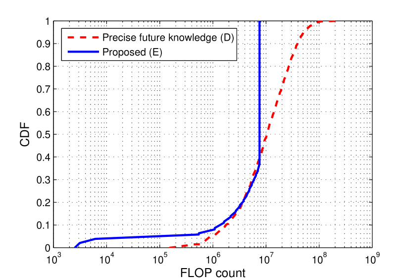
Figure 7: Cumulative distribution functions (CDF) of computation time and FLOP count.

We study the computational overhead of the proposed algorithm for obtaining service configurations corresponding to the results shown in Fig. 6(a). The simulations were run in MATLAB on a laptop with Intel(R) Core(TM) i5-4300U CPU, 4 GB memory, and 64-bit Windows 10. We focus on the computation time and amount of floating-point operations (FLOP) for every computation of the next $T$-slot configuration for one instance. We compare the performance between the proposed approach (E) and the precise future knowledge scenario (D). We do not compare against MMC-only and backend cloud-only approaches (A, B, and C) because those approaches are much simpler but produce a significantly higher cost than approaches D and E (see Fig. 6(a)) thus it is not fair to compare their computational overheads. The FLOP counts are obtained using the toolbox in [A1] (references for appendices are listed at the end of this document).

We collected statistics of the computation time and FLOP count for each execution of the algorithm to compute the next $T$-slot configuration when using approaches D and E. Fig. 7 shows the cumulative distribution function (CDF), where $\textrm{CDF}(x)$ is defined as the percentage of observations (i.e., computation time or FLOP count) that has a value smaller than or equal to $x$. Table II lists the sum (for all executions), mean, standard deviation, and maximum values.

We see that in terms of computation time, the proposed approach (E) can find the configuration within $1.84$ s on average. Recalling that each timeslot corresponds to a physical time of $60$ s and the configuration for multiple timeslots is usually found by a single execution of the algorithm, the time needed for running the algorithm is relatively short.

We note that because we ran the simulation in MATLAB and our code is not optimized for performance, our results are pessimistic and the algorithm should run much faster with a better optimized code written in C, for instance. This can be seen by the fact that the average FLOP count of the proposed approach is only $6.08\times 10^{6}$ while modern personal computers can easily complete over $10^{9}$ floating-point operations per second (FLOPS), see the experimental results in [A2] for example. Server machines will be even more powerful. This means that if we fully utilize the resource of a personal computer, the proposed algorithm should be able to find the configuration (for a single instance) within $0.01$ s. Such a timescale will be sufficient for deploying newly arrived instances on the cloud in real time. From this FLOP count comparison, we can conclude that the proposed algorithm only consumes a small amount of processing capability, so it is applicable in practice and scalable to a reasonably large amount of users.

We further note that the proposed algorithm may benefit from parallelization and performing the computation on GPUs. For example, parallelization is possible for the “for all” loops between Lines 6 and 9 and also between Lines 10 and 15 in Algorithm 2. This can further expedite the process of finding configurations.

Comparing approach D with the proposed approach (E), Table II shows that the mean, standard deviation, and maximum values of the proposed approach is lower than those of approach D. This is because the proposed approach uses the optimal look-ahead window size, which is usually much smaller than the total number of timeslots in which the instance remains active, whereas approach D is assumed to have precise knowledge of the future and therefore takes into account the entire duration in which the instance is active. According to the complexity analysis in Section 3.3, considering more timeslots in the optimization causes higher algorithmic complexity, thus explaining the result.

When looking at the sum values in Table II, the proposed approach has a similar but slightly larger computation time and FLOP count than approach D. This is because approach D is assumed to know exactly when an instance departs from the system, whereas the proposed approach does not have this knowledge and may consider additional slots after instance departure as part of the optimization process. However, the gap is not large because the proposed approach has a relatively small look-ahead window; the instance departure becomes known to the proposed approach at the beginning of a new look-ahead window.

The fact that the mean and maximum values (in Table II) of the proposed approach are much smaller than those of approach D also makes the proposed approach more suitable for real-time requests, because it can apply a configuration quickly after instance arrival. More importantly, we recall that approach D is impractical because it assumes precise prediction of future costs and instance departure times.

References for Appendices

1. H. Qian, “Counting the Floating Point Operations (FLOPS),” MATLAB Central File Exchange, No. 50608, available at http://www.mathworks.com/matlabcentral/fileexchange/50608

2. MaxxPI² – the System Bench, http://www.maxxpi.net/pages/result-browser/top15---flops.php

References

- [1] S. Wang, R. Urgaonkar, K. Chan, T. He, M. Zafer, and K. K. Leung, “Dynamic service placement for mobile micro-clouds with predicted future cost,” in Proc. of IEEE ICC 2015, Jun. 2015.
- [2] M. Satyanarayanan, Z. Chen, K. Ha, W. Hu, W. Richter, and P. Pillai, “Cloudlets: at the leading edge of mobile-cloud convergence,” in Proc. of MobiCASE 2014, Nov. 2014.
- [3] “Smarter wireless networks,” IBM Whitepaper No. WSW14201USEN, Feb. 2013. [Online]. Available: www.ibm.com/services/multimedia/Smarter\_wireless\_networks.pdf
- [4] M. Satyanarayanan, R. Schuster, M. Ebling, G. Fettweis, H. Flinck, K. Joshi, and K. Sabnani, “An open ecosystem for mobile-cloud convergence,” IEEE Communications Magazine, vol. 53, no. 3, pp. 63–70, Mar. 2015.
- [5] T. Taleb and A. Ksentini, “Follow me cloud: interworking federated clouds and distributed mobile networks,” IEEE Network, vol. 27, no. 5, pp. 12–19, Sept. 2013.
- [6] S. Davy, J. Famaey, J. Serrat-Fernandez, J. Gorricho, A. Miron, M. Dramitinos, P. Neves, S. Latre, and E. Goshen, “Challenges to support edge-as-a-service,” IEEE Communications Magazine, vol. 52, no. 1, pp. 132–139, Jan. 2014.
- [7] Z. Becvar, J. Plachy, and P. Mach, “Path selection using handover in mobile networks with cloud-enabled small cells,” in Proc. of IEEE PIMRC 2014, Sept. 2014.
- [8] A. Fischer, J. Botero, M. Beck, H. De Meer, and X. Hesselbach, “Virtual network embedding: A survey,” IEEE Commun. Surveys Tuts., vol. 15, no. 4, pp. 1888–1906, 2013.
- [9] M. Chowdhury, M. Rahman, and R. Boutaba, “Vineyard: Virtual network embedding algorithms with coordinated node and link mapping,” IEEE/ACM Transactions on Networking, vol. 20, no. 1, pp. 206–219, 2012.
- [10] A. Ksentini, T. Taleb, and M. Chen, “A Markov decision process-based service migration procedure for follow me cloud,” in Proc. of IEEE ICC 2014, Jun. 2014.
- [11] S. Wang, R. Urgaonkar, T. He, M. Zafer, K. Chan, and K. K. Leung, “Mobility-induced service migration in mobile micro-clouds,” in Proc. of IEEE MILCOM 2014, Oct. 2014.
- [12] S. Wang, R. Urgaonkar, M. Zafer, T. He, K. Chan, and K. K. Leung, “Dynamic service migration in mobile edge-clouds,” in Proc. of IFIP Networking 2015, May 2015.
- [13] M. Srivatsa, R. Ganti, J. Wang, and V. Kolar, “Map matching: Facts and myths,” in Proc. of ACM SIGSPATIAL 2013, 2013, pp. 484–487.
- [14] A. Borodin and R. El-Yaniv, Online Computation and Competitive Analysis. Cambridge University Press, 1998.
- [15] S. O. Krumke, Online optimization: Competitive analysis and beyond. Habilitationsschrift Technische Universitaet Berlin, 2001.
- [16] Y. Azar, I. R. Cohen, and D. Panigrahi, “Online covering with convex objectives and applications,” CoRR, vol. abs/1412.3507, Dec. 2014. [Online]. Available: http://arxiv.org/abs/1412.3507
- [17] N. Buchbinder, S. Chen, A. Gupta, V. Nagarajan, and J. Naor, “Online packing and covering framework with convex objectives,” CoRR, vol. abs/1412.8347, Dec. 2014. [Online]. Available: http://arxiv.org/abs/1412.8347
- [18] R. Urgaonkar, S. Wang, T. He, M. Zafer, K. Chan, and K. K. Leung, “Dynamic service migration and workload scheduling in edge-clouds,” Performance Evaluation, vol. 91, pp. 205–228, Sept. 2015, to be presented at IFIP Performance 2015.
- [19] H.-C. Hsiao, H.-Y. Chung, H. Shen, and Y.-C. Chao, “Load rebalancing for distributed file systems in clouds,” IEEE Trans. on Parallel and Distributed Systems, vol. 24, no. 5, pp. 951–962, 2013.
- [20] Y. Azar, “On-line load balancing,” Theoretical Computer Science, pp. 218–225, 1992.
- [21] J. Li, H. Kameda, and K. Li, “Optimal dynamic mobility management for pcs networks,” IEEE/ACM Trans. Netw., vol. 8, no. 3, pp. 319–327, Jun. 2000.
- [22] J. Li and H. Kameda, “Load balancing problems for multiclass jobs in distributed/parallel computer systems,” IEEE Transactions on Computers, vol. 47, no. 3, pp. 322–332, Mar. 1998.
- [23] C.-H. Chen, S. D. Wu, and L. Dai, “Ordinal comparison of heuristic algorithms using stochastic optimization,” IEEE Trans. on Robotics and Automation, vol. 15, no. 1, pp. 44–56, 1999.
- [24] J. Aspnes, Y. Azar, A. Fiat, S. Plotkin, and O. Waarts, “On-line routing of virtual circuits with applications to load balancing and machine scheduling,” J. ACM, vol. 44, no. 3, pp. 486–504, May 1997.
- [25] G. Aceto, A. Botta, W. de Donato, and A. Pescape, “Cloud monitoring: A survey,” Computer Networks, vol. 57, no. 9, pp. 2093 – 2115, 2013.
- [26] E. Cho, S. A. Myers, and J. Leskovec, “Friendship and mobility: User movement in location-based social networks,” in Proc. of the 17th ACM SIGKDD International Conference on Knowledge Discovery and Data Mining, ser. KDD ’11, 2011, pp. 1082–1090.
- [27] K. LaCurts, J. Mogul, H. Balakrishnan, and Y. Turner, “Cicada: Introducing predictive guarantees for cloud networks,” Jun. 2014.
- [28] W. B. Powell, Approximate Dynamic Programming: Solving the curses of dimensionality. John Wiley & Sons, 2007.
- [29] B. Korte and J. Vygen, Combinatorial optimization. Springer, 2002.
- [30] S. Boyd and L. Vandenberghe, Convex optimization. Cambridge university press, 2004.
- [31] M. Piorkowski, N. Sarafijanovoc-Djukic, and M. Grossglauser, “A parsimonious model of mobile partitioned networks with clustering,” in Proc. of COMSNETS, Jan. 2009.
- [32] M. Piorkowski, N. Sarafijanovic-Djukic, and M. Grossglauser, “CRAWDAD data set epfl/mobility (v. 2009-02-24),” Downloaded from http://crawdad.org/epfl/mobility/, Feb. 2009.