Attitude Estimation and Control Using Linear-Like Complementary Filters: Theory and Experiment

Abstract

This paper proposes new algorithms for attitude estimation and control based on fused inertial vector measurements using linear complementary filters principle. First, $n$-order direct and passive complementary filters combined with TRIAD algorithm are proposed to give attitude estimation solutions. These solutions which are efficient with respect to noise include the gyro bias estimation. Thereafter, the same principle of data fusion is used to address the problem of attitude tracking based on inertial vector measurements. Thus, instead of using noisy raw measurements in the control law a new solution of control that includes a linear-like complementary filter to deal with the noise is proposed. The stability analysis of the tracking error dynamics based on LaSalle’s invariance theorem proved that almost all trajectories converge asymptotically to the desired equilibrium. Experimental results, obtained with DIY Quad equipped with the APM2.6 auto-pilot, show the effectiveness and the performance of the proposed solutions.

I Introduction

Most of traditional rigid body attitude control approaches given in the literature are based on feedback scheme using attitude estimation (see e.g. [1, 2, 3, 4, 5]). Recently, some authors propose to use directly raw vector measurements to perform attitude control (see e.g. [6, 7, 8]). In fact, the explicit use of the attitude in the control law involves the determination of attitude from measurements provided by appropriate sensors. It is known that there are no sensors directly measuring the attitude but it can be determined from measurements in the body frame using suitable algorithms (see e.g. [9, 10, 11, 12, 13]). Almost all attitude control applications use measurement data from embedded Inertial Measurement Units (IMU). The capability of the rigid body to track desired attitude trajectories depends on the reliability of these sensors and the quality of measurements related to sensitivity to noise, bias, etc. To take into account the sensor imperfections, many techniques of attitude estimation and control were developed. For instance, as mentioned in the survey paper [14], the problem of attitude estimation is generally treated in two steps, estimation of the attitude with raw measurements and filtering. The most and widely used techniques in this case are based on extended Kalman filter [14, 15]. Some other techniques are developed like the nonlinear observer given in [16], or based on unscented filter [17]. Most of these methods are computationally demanding and some of them, depending on used attitude representation [18], suffer from topological limitations, double covering or singularities. Another class of techniques are based on complementary filters [19, 20] which are not so computationally demanding, see [21] for comparison between complementary and Kalman filtering.

Due to their simplicity and efficiency, the use of complementary filters to reconstruct the attitude continues to attract many researchers. A lot of them focus on low-cost IMU and attitude heading reference system AHRS [22]. Nonlinear complementary filters designed on Special Orthogonal Group $SO(3)$ [23] and on the unit 3-sphere $\mathbb{S}^{3}$ [24] were used successfully to estimate the attitude. Modified complementary filters using only accelerometer and gyroscope measurements to estimate the orientation was presented in [25]. Another recent work has used the inverse sensor models and complementary filters to develop a high-fidelity attitude estimator [26]. As mentioned in [27], traditional attitude solutions use directly raw vector measurements to compute the attitude data after that the observer is used to estimate the attitude. [27] proposed a reverse strategy by combining a vector-based filter with an optimal attitude determination algorithm, in which the distortion of noise characteristics is avoided. A new interesting class of globally asymptotically stable filters for attitude estimation was obtained. The vector-based filter was designed as a Kalman filter using Linear Time Variant (LTV) representation of the nonlinear kinematic equation. Even if experimental results presented in [27] are very good, the theoretical drawback is the fact that the observability conclusions were given for the LTV reformulation of the original nonlinear system and not explicitly on the non linear system.

Inspired by approach given in [27], this paper presents firstly globally asymptotically stable filters for attitude estimation based on high order linear complementary filtering. The gyro-bias estimation is also considered. Two forms of filter, termed “direct” and “passive”, are designed similarly as the work presented in [23]. The passive form is less sensitive to noise as claimed in [23]. Moreover, the approach proposed here is completely deterministic as it is based on linear complementary filters followed by TRIAD algorithm for the attitude estimation. As a matter of fact, the TRIAD is the deterministic attitude estimation algorithm par excellence as claimed by [28]. Although it was proved that TRIAD is less accurate than other optimal approaches [28], we show throughout this work that it is possible to obtain higher quality of the attitude estimation when this approach is used.

The quality of IMU measurements is much degraded by the phenomenon of vibrations of the real system. Frequently, the implementations of some attitude controllers using directly raw vector measurements are confronted with this phenomenon. Therefore, we propose to use a new filter to improve the performance of the attitude tracking controller. The proposed attitude controller is based on the filtered vector measurements instead of the raw ones, while ensuring an almost global stability without using “attitude measurements”.

The result presented in this paper extends those from [29]. The first contribution of this work is the extension of the global convergence of the direct complementary filters to the case of n-order. Also, we propose general n-order passive filters, where we obtain the global asymptotic convergence to zero of the estimation errors. This constitutes our second contribution. Another contribution is the design of a new control law based only on inertial and rate-gyro measurements to control the attitude of a rigid body without using “attitude measurements”, for which an almost global stability is given. All our contributions are validated by experiments on the DIY drone Quad-copter [30].

II Preliminaries

II-A Mathematical background and Notations

Consider a rigid-body moving in 3D space with orthonormal body-frame $\left\{\mathcal{B}\right\}$ fixed to its center of gravity and denote by $\left\{\mathcal{I}\right\}$ the inertial reference frame attached to the 3D space. Attitude of the rigid body represents the relative orientation of the $\left\{\mathcal{B}\right\}$ with respect to $\left\{\mathcal{I}\right\}$. It can be represented using several mathematical models. Representing the attitude by rotation matrix $R$, provides an unique, global and non singular parametrization of the orientation [18]. The rotation matrix is an element of the special orthogonal group $SO(3)$ with $SO(3)=\{R\in\mathcal{\mathrm{\mathbb{R}}}^{3\times 3}\mid R^{T}R=RR^{T}=I_{3},\,\det(R)=1\}$ where $I_{3}$ is the $3\times 3$ identity matrix. The associated Lie algebra denoted by $\mathfrak{so}(3)$ is the set of skew symmetric matrices such that $\mathfrak{so}(3)=\{A\in\mathcal{\mathrm{\mathbb{R}}}^{3\times 3}\mid A=-A^{T}\}$. Denote by $S$ the Lie algebra mapping from $\mathbb{R}^{3}\rightarrow\mathfrak{so}(3)$ which associates to $x\in\mathbb{R}^{3}$ the skew-symmetric matrix $S(x)$, such that

$$S(x)=\left[\begin{array}[]{ccc}0&-x_{z}&x_{y}\\ x_{z}&0&-x_{x}\\ -x_{y}&x_{x}&0\end{array}\right]\;and\;x=\left[\begin{array}[]{c}x_{x}\\ x_{y}\\ x_{z}\end{array}\right]$$ (1)

For any two vectors $x,\,y\in\mathbb{R}^{3}$ and rotation matrix $R\in SO(3)$, the following identities hold:

$$\begin{cases}S(x)y&=x\times y=-S(y)x,\\ S(S(x)y)&=S(x)S(y)-S(y)S(x),\\ S(x)^{2}&=xx^{T}-x^{T}xI_{3},\\ S(Rx)&=RS(x)R^{T},\end{cases}$$ (2)

where $\times$ denotes the vector cross product.

Another global and non singular parametrization of the attitude is described by unit quaternion $Q$ which is an element of unit sphere $\mathbb{S}^{3}=\left\{Q=\left(q_{0},q^{T}\right)^{T}\text{, }q_{0}\in\mathbb{R},\text{\ }q\in\mathbb{R}^{3},\text{ }q_{0}^{2}+q^{T}q=1\right\}$. The multiplication of two quaternions $P=(p_{0},p^{T})^{T}$ and $Q=(q_{0},q^{T})^{T}$ is denoted by “$\odot$” and defined as $P\odot Q=\left[\begin{array}[]{c}p_{0}q_{0}-p^{T}q\\ p_{0}q+q_{0}p+p\times q\end{array}\right]$ and for any unit quaternion $Q=(q_{0},q^{T})^{T}$, we have $Q\odot Q^{-1}=Q^{-1}\odot Q=(1,\mathbf{0})$, where $Q^{-1}=(q_{0},-q^{T})^{T}$.

Both $Q\in\mathbb{S}^{3}$ and $R\in SO(3)$ are related to each other through the mapping $\mathcal{R}:\mathbb{S}^{3}\rightarrow SO(3)$ by the Euler-Rodriguez formula as follows:

$$\begin{array}[]{c}\mathcal{R}(Q)=I_{3}+2q_{0}S(q)+2S(q)^{2}\end{array}$$ (3)

If $n$ is a positive integer, set $e_{n}=(0,\cdots,0,1)^{T}$. To every $\gamma=(\gamma_{1},\ldots,\gamma_{n})\in\mathbb{R}^{n}$, we associate the polynomial

$$P_{\gamma}(s)=s^{n}+\sum_{k=1}^{n}\gamma_{k}s^{n-k},$$ (4)

and the companion matrix $A_{\gamma}$

$$A_{\gamma}=\left(\begin{array}[]{ccccc}0&1&0&\cdots&0\\ 0&0&1&\ddots&\vdots\\ \vdots&\vdots&0&\ddots&\vdots\\ \vdots&\vdots&\vdots&\ddots&0\\ 0&0&\cdots&0&1\\ -\gamma_{n}&-\gamma_{n-1}&\cdots&-\gamma_{2}&-\gamma_{1}\end{array}\right)$$ (5)

whose characteristic polynomial is $P_{\gamma}$. Use $\pi:\mathbb{R}^{n}\rightarrow\mathbb{R}^{n-1}$ to denote the projection onto $\mathbb{R}^{n-1}$ i.e., $\pi(\gamma)=(\gamma_{1},\cdots,\gamma_{n-1})$. Define the following subsets of $\mathbb{R}^{n}$,

$$\mathcal{H}_{n}=\left\{\gamma\in\mathbb{R}^{n}\,\mid\,P_{\gamma}\;Hurwitz\right\},\quad\mathcal{\overline{H}}_{n}=\left\{\gamma\in\mathcal{H}_{n}\,\mid\,\pi(\gamma)\in\mathcal{H}_{n-1}\right\}.$$

The proof of the following lemma is defereed in Appendix.

Lemma 1.

If $n$ is a positive integr, then $\mathcal{\overline{H}}_{n}$ is not empty.

Note 1.

Let $E\in\mathbb{R}^{(n\times n)}$ and $\sigma(E)=\left\{\lambda_{1},\ldots,\lambda_{n}\right\}$ its spectrum, where $\lambda_{l},\,l=1\ldots n$ are the eigenvalues of $E$. Let $I_{k}\in\mathbb{R}^{(k\times k)}$, $k$ integer, be the identity matrix. Then, the spectrum of the Kronecker product of $E$ by $I_{k}$, $E\otimes I_{k}\in\mathbb{R}^{(kn\times kn)}$, is equal to $\sigma(E)$ according to Theorem in page 245 of [31]. In particular, $E\otimes I_{k}$ is Hurwitz if and only $E$ is.

II-B Attitude kinematics, Dynamics and Assumptions

The rigid body rotational motion can be described by its kinematic and dynamic equations. Using the rotation matrix representation, the rigid body attitude is governed by the following kinematic equation

$$\dot{R}(t)=R(t)S(\omega(t)),$$ (6)

where $\omega(t)$ being the angular velocity of the rigid body expressed in $\left\{\mathcal{B}\right\}$. Equivalently in term of unit quaternion, we can have $\dot{Q}(t)=\frac{1}{2}Q(t)\odot\bar{\omega}(t)$ with $\bar{\omega}(t)$ is the pure quaternion defined by $\bar{\omega}(t)=(0,\omega(t)^{T})^{T}$, which gives

$$\dot{Q}(t)=\left[\begin{array}[]{c}\dot{q}_{0}(t)\\ \dot{q}(t)\end{array}\right]=\left[\begin{array}[]{c}-\frac{1}{2}q^{T}(t)\omega(t)\\ \frac{1}{2}(q_{0}(t)I_{d}+S(q(t)))\omega(t)\end{array}\right],$$ (7)

Now, given a constant vector $r$ in inertial $\left\{\mathcal{I}\right\}$, then its corresponding vector in the $\left\{\mathcal{B}\right\}$ is given by $b(t)=R^{T}(t)r$. Thus, using (6), one can get the following reduced attitude kinematics

$$\dot{b}(t)=-S(\omega(t))b(t)$$ (8)

By considering applied torque $\tau(t)$ to the system expressed in $\left\{\mathcal{B}\right\}$, the rigid body simplified rotational dynamics is governed by

$$\begin{array}[]{c}J\dot{\omega}(t)=-S(\omega(t))J\omega(t)+\tau(t),\end{array}$$ (9)

where $J\in\mathbb{R}^{3\times 3}$ is a symmetric positive definite constant inertia matrix of the rigid body with respect to $\left\{\mathcal{B}\right\}$.

Consider the following rate-gyros model

$$\omega_{m}(t)=\omega(t)+\eta,$$ (10)

where $\omega_{m}(t)$ is the measured angular velocity and $\eta$ is the real unknown gyro-bias.

Along this work, we use the following assumptions :

Assumption 1.

We assume that, if we have $m$ measured vectors $b_{i}(t),\,i=1,...,m$ expressed in $\left\{\mathcal{B}\right\}$, corresponding to $m$ inertial constant vectors $r_{i},\,i=1,...,m$ expressed in $\left\{\mathcal{I}\right\}$, then at least two of them are non-collinear.

Assumption 2.

We assume that the real unknown gyro-bias $\eta$ is bounded and constant (or slowly varying), such that $\dot{\eta}=0$. Moreover, we assume that we are dealing with bounded measured angular velocities $\omega_{m}(\cdot)$, implying that the real angular velocity $\omega(\cdot)$ is bounded as well.

Using the reduced attitude kinematics (8) and the model of the rate-gyro (10), we can write the following system

$$\begin{cases}\begin{array}[]{lcl}\dot{b}_{i}&=&-S(\omega_{m}-\eta)b_{i}\\ \dot{\eta}&=&0.\end{array}\end{cases},$$ (11)

where $i=1,...,m$. Note that, in all what follows the indices $i=1,...,m$ denote the number of the used inertial vectors.

II-C Complementary linear filter-based attitude estimation approach

The sensor-based attitude estimation approach [27] is consisting of two processes: i) filtering sensor measurements, and ii) determining attitude. Inspired by this approach, we propose a structure based on complementary linear filter rather than sensor-based filter method. Indeed, complementary filters give us a mean to fuse multiple heterogeneous independent noisy measurements of the same signal that have complementary spectral characteristics [23]. By developing a high-fidelity and simple algorithm for attitude estimation, the proposed structure must allow the possibility of using high order filter which leads to better performance.

Using the reduced attitude kinematics (8), the complementary filter model for fusing the measured inertial vector $b_{i}(t)$ and gyros measurements $\omega_{m}$ in order to get estimate $\hat{b}_{i}(t)$ is shown in Figure 1, where the notion of complementary filter is achieved if the following condition is satisfied

$$H_{1i}(s)+sH_{2i}(s)=1,\quad i=1,\cdots,m,$$ (12)

where $H_{1i}(s)$ is a low-pass filter and $sH_{2i}(s)$ is a high-pass filter.

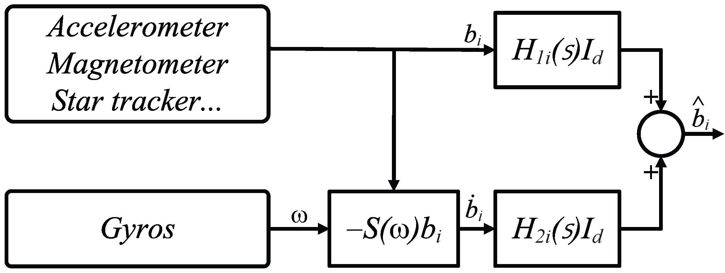
Figure 1: Classical form of complementary filter

From the structure of the complementary filter given in Figure 1, the estimate $\hat{b}_{i}$ of the state $b_{i}$ by fusing measurements of $i\,th$ inertial direction vector and gyro measurements can be write as

$$\hat{b}_{i}=H_{1i}(s)b_{i}+H_{2i}(s)\dot{b}_{i},\quad i=1,\cdots,m.$$ (13)

Now, for the determination of the attitude, the complementary filter can will be followed by a TRIAD algorithm [10]. Despite the fact that TRIAD is known less accurate than other statistical algorithms based on minimizing Wahba’s loss function [28], we will show that we can obtain good results by using fused data. The choice of TRIAD algorithm is justified by the fact that optimal algorithms are usually much slower than deterministic algorithms [10, 28].

The first problem addressed in this work is the design of an attitude and heading reference system using the concept of sensor-based attitude estimation approach [27]. The goal is to proof that it is possible to obtain a structure based on complementary linear filter with a globally asymptotic convergence. The filtered data will be used by a TRIAD for attitude determination as explained before.

The second problem addressed is to proof that the use of estimated measurements by complementary filters can achieve attitude tracking with an almost global stability.

III Design of High Order Direct and Passive Filters with Gyro-Bias Estimation

The principle of the “classical form” of complementary filters is based on the data fusion of measurements of inertial direction vectors and gyro measurements as depicted by the scheme of Figure 1. This scheme can be reformulated in “feedback form” as shown by Figure 2. Furthermore, according to the manner of offsetting the nonlinear term, we can obtain two structures of the complementary filter. The first one is termed “direct linear complementary filter” and the second one termed “passive linear-like complementary filter” . Indeed, in the first one, the offsetting of nonlinear term uses direct raw measurements as shown in Figure 2 while in the second one, the filtered measurements are used as depicted in Figure 3.

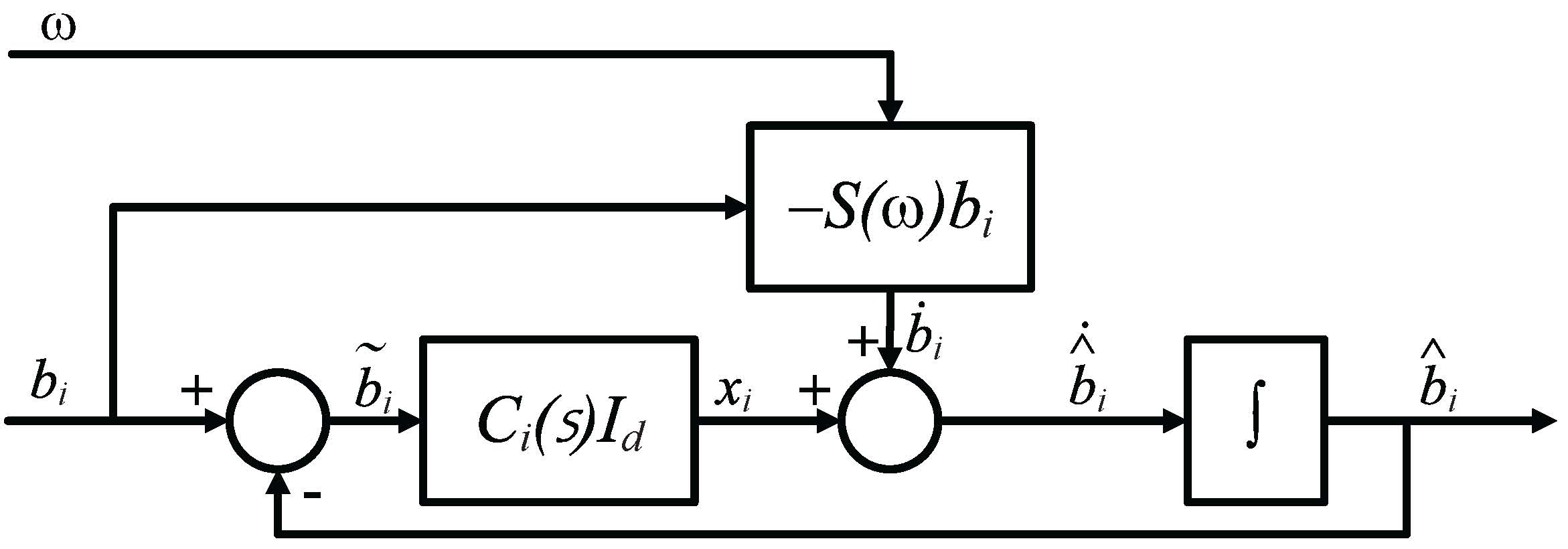
Figure 2: Direct linear complementary filter

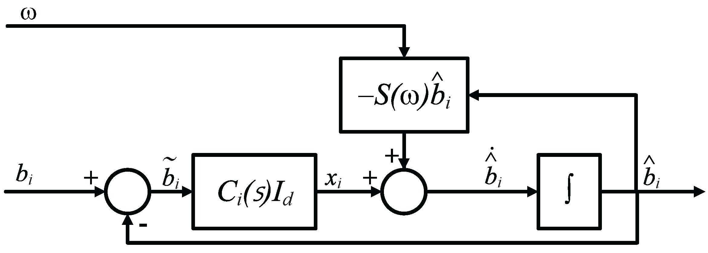
Figure 3: Passive linear-like complementary filter

From the equivalence between the “classical form” and the “feedback form”, one can get

$$H_{1i}\left(s\right)=\frac{C_{i}\left(s\right)}{s+C_{i}\left(s\right)},\;H_{2i}\left(s\right)=\frac{1}{s+C_{i}\left(s\right)},\,i=1,...,m,$$ (14)

where $C_{i}(s)$ represents the compensator term in the feedback form. From (14), we can write the compensator term as

$$C_{i}(s)=\frac{sH_{1i}(s)}{1-H_{1i}(s)},\,i=1,...,m.$$ (15)

The design of the compensator $C_{i}(s)$ can be achieved by choosing the adequate filter order for improving the quality of estimation. Consider now, for $i=1\cdots,m,$ the general $n$-order transfer function $H_{1i}(s)$ by first taking $\varUpsilon_{i}\in\mathcal{H}_{n}$ and setting

$$H_{1i}(s)=\frac{\gamma_{in}}{P_{\varUpsilon_{i}}(s)},$$ (16)

where $P_{\varUpsilon_{i}}(s)$ and $\gamma_{in}$ are defined by (4). Using (15) one can get

$$C_{i}(s)=\frac{\gamma_{in}}{P_{\varPi(\varUpsilon_{i})}(s)},\,i=1,...,m.$$ (17)

III-A High-Order Direct Linear Complementary Filters

Consider System (11) and the block diagram of the direct form in Figure 2 with compensator $C_{i}(s)$ given by (17) for $i=1,...,m$. Then, the closed-loop dynamics with gyro bias estimation for any $n$-order is given for $i=1,...,m$ by

$$\begin{cases}\begin{array}[]{lcl}x_{i}^{(n-1)}&=&-\sum_{k=1}^{n-1}\gamma_{ik}x_{i}^{(n-k-1)}+\gamma_{in}(b_{i}-\hat{b}_{i}),\\ \dot{\hat{b}}_{i}&=&-S(\omega_{m}-\hat{\eta})b_{i}+x_{i},\\ \dot{\hat{\eta}}&=&\Gamma_{d}\sum_{i=1}^{m}S(b_{i})\upsilon_{i}\end{array}\end{cases},$$ (18)

where $x_{i}^{(j)}$ is the $j-$th derivative of $x_{i}$ with $x_{i}^{(0)}=x_{i}$, $\gamma_{ik},\,i=1,...,m,\,k=1,...,n$ are components of $\varUpsilon_{i}\in\mathcal{H}_{n}$, $\Gamma_{d}$ is a real positive definite diagonal matrix gain and $\upsilon_{i}$ is a vector to be defined later.

Define the observation errors

$$\widetilde{b}_{i} = b_{i}-\hat{b}_{i},\,i=1,...,m,$$ (19)

$$\widetilde{\eta} = \eta-\hat{\eta},$$ (20)

then using (8) and (18)-(20), yield the following error dynamics

$$\begin{cases}\begin{array}[]{lcl}x_{i}^{(n-1)}&=&-\sum_{k=1}^{n-1}\gamma_{ik}x_{i}^{(n-k-1)}+\gamma_{in}\tilde{b}_{i},\\ \dot{\widetilde{b}}_{i}&=&-S(b_{i})\widetilde{\eta}-x_{i},\\ \dot{\widetilde{\eta}}&=&-\Gamma_{d}\sum_{i=1}^{m}S(b_{i})\upsilon_{i}.\end{array}\end{cases}$$ (21)

By the evaluation of the time derivative of the first equation of (21), one can rewrite (21) as

$$\begin{cases}\begin{array}[]{lcl}x_{i}^{(n)}&=&-\sum_{k=1}^{n}\gamma_{ik}x_{i}^{(n-k)}-\gamma_{in}S(b_{i})\widetilde{\eta}\\ \dot{\widetilde{\eta}}&=&-\Gamma_{d}\sum_{i=1}^{m}S(b_{i})\upsilon_{i}\end{array}\end{cases}$$ (22)

Now, consider the new state vector $z_{i}\in\mathbb{R}^{3n},\,i=1,...,m$ such as $z_{i}^{T}=\left[x^{T},\dot{x}^{T},\cdots,x^{(n-1)T}\right]$ and define the vectors $\upsilon_{i}$ to be

$$\upsilon_{i}=B_{di}^{T}P_{di}z_{i},\,i=1,...,m.$$ (23)

One can rewrite (22) as

$$\begin{cases}\begin{array}[]{lcl}\dot{z}_{i}(t)&=&A_{di}z_{i}(t)+B_{di}S(\widetilde{\eta})b_{i},\\ \dot{\widetilde{\eta}}&=&-\Gamma_{d}\sum_{i=1}^{m}S(b_{i})B_{di}^{T}P_{di}z_{i},\end{array}\end{cases}$$ (24)

where $i=1,...,m$, the Hurwitz matrices $A_{di}=A_{\varUpsilon_{i}}\otimes I_{d}\in\mathbb{R}^{(3n\times 3n)}$ ($A_{\varUpsilon_{i}}$ is defined by (5)), $B_{di}=\gamma_{in}e_{n}\otimes I_{3}\in\mathbb{R}^{3n\times 3}$ and the matrices $P_{di}\in\mathbb{R}^{(3n\times 3n)},\,i=1,...,m$, are real symmetric positive definite solutions of the following Lyapunov equations for given symmetric positive definite matrices $Q_{di}$

$$A_{di}^{T}P_{di}+P_{di}A_{di}=-Q_{di},\,i=1,...,m$$ (25)

We can now state our first result.

Proposition 1.

Consider the filter (18) and (23), under Assumptions 1 and 2 in subsection II-B. Then the errors (19) and (20) converge globally asymptotically to zero.

Proof.

Consider the following Lyapunov function candidate

$$V_{1}=\sum_{i=1}^{m}z_{i}^{T}P_{di}z_{i}+\widetilde{\eta}^{T}\Gamma_{d}^{-1}\widetilde{\eta}$$ (26)

where $P_{di}\in\mathbb{R}^{(3n\times 3n)},\,i=1,...,m$ is given by (25). The time derivative of (26) in view of (24) is given by

$$\begin{array}[t]{ccl}\dot{V}_{1}&=&\sum_{i=1}^{m}\left(z_{i}^{T}P_{di}\dot{z}_{i}+\dot{z}_{i}^{T}P_{di}z_{i}\right)+\widetilde{\eta}^{T}\Gamma_{d}^{-1}\dot{\widetilde{\eta}},\\ &=&\sum_{i=1}^{m}\left(z_{i}^{T}\left(A_{di}^{T}P_{di}+P_{di}A_{di}\right)z_{i}+2z_{i}^{T}P_{di}B_{di}S(\widetilde{\eta})b_{i}\right)-2\widetilde{\eta}^{T}\sum_{i=1}^{m}S(b_{i})B_{di}^{T}P_{di}z_{i},\end{array}$$

using (25) and the fact that $\widetilde{\eta}^{T}S(b_{i})B_{di}^{T}P_{di}z_{i}=z_{i}^{T}P_{di}B_{di}S(\widetilde{\eta})b_{i}$, then

$$\dot{V}_{1}=-\sum_{i=1}^{m}z_{i}^{T}Q_{di}z_{i}\leqslant 0.$$ (27)

Therefore $z_{i}$ and $\widetilde{\eta}_{i}$ are bounded and consequently by using (24), $\dot{z}_{i}$ and $\dot{\widetilde{\eta}}_{i}$ are bounded. The evaluation of the second derivative of (26) in view of (24) gives

$$\ddot{V}_{1} = -\sum_{i=1}^{m}z_{i}^{T}\left(A_{di}^{T}Q_{di}+Q_{di}A_{di}\right)z_{i}+2z_{i}^{T}Q_{di}B_{di}S(b_{i})\widetilde{\eta},$$ (28)

which is clearly bounded. By Barbalat’s lemma, ${\displaystyle\lim_{t\rightarrow\infty}\dot{V}_{1}(t)=0}$ and consequently ${\displaystyle\lim_{t\rightarrow\infty}z_{i}(t)=0}$. Then, according to (21), one can obtain ${\displaystyle\lim_{t\rightarrow\infty}\widetilde{b}_{i}(t)=0}$. The second time derivative of $z_{i}$ is given by

$$\ddot{z}_{i}=A_{di}\left(A_{di}z_{di}(t)+B_{di}S(b_{i})\widetilde{\eta}\right)+B_{di}S(S(b_{i})\omega)\widetilde{\eta}+B_{di}S(b_{i})\dot{\widetilde{\eta}},$$ (29)

where all terms are bounded. Thus using Barbalat’s lemma, ${\displaystyle\lim_{t\rightarrow\infty}\dot{z}_{i}(t)=0}$. Therefore, using (24) and ${\displaystyle\lim_{t\rightarrow\infty}z_{i}(t)=0}$, one can conclude that $B_{di}S(b_{i})\widetilde{\eta}$ converge to zero and equivalently ${\displaystyle\lim_{t\rightarrow\infty}S(b_{i}(t))\widetilde{\eta}(t)=0}$. Under Assumption 1, one can conclude that ${\displaystyle\lim_{t\rightarrow\infty}\widetilde{\eta}(t)=0}$. ∎

Remark 1.

Substituting the value of $n$ by 1 in (18), and after some manipulations, one can obtain the first order direct filter as

$$\begin{cases}\begin{array}[]{lcl}\dot{\hat{b}}_{i}&=&-S(\omega_{m}-\hat{\eta})b_{i}+\gamma_{i1}(b_{i}-\hat{b}_{i})\\ \dot{\hat{\eta}}&=&\Gamma_{1}\sum_{i=1}^{m}S(b_{i})\hat{b}_{i}\end{array}\end{cases},$$ (30)

III-B High-Order Passive Linear-like Filters

In the passive form, the design of the complementary filter is performed by injecting filtered measurements for offsetting nonlinear term as shown in block diagram of Figure 3 with a compensator $C_{i}(s)$, $i=1,\cdots,m$, defined by (17). Then, we propose the following new $n$-order passive form with gyro bias estimation

$$\begin{cases}\begin{array}[]{lcl}x_{i}^{(n-1)}&=&-\sum_{k=1}^{n-1}\gamma_{ik}x_{i}^{(n-k-1)}+\gamma_{in}(b_{i}-\hat{b}_{i}),\\ \dot{\hat{b}}_{i}&=&-S(\omega_{m}-\hat{\eta})\hat{b}_{i}+w_{i},\\ \dot{\hat{\eta}}&=&-\Gamma_{p}\sum_{i=1}^{m}S(b_{i})\hat{b}_{i},\end{array}\end{cases},$$ (31)

where $i=1,...,m$, $x_{i}^{(j)}$ is the $j\,th$ order derivative of $x_{i}$ with $x_{i}^{(0)}=x_{i}$, $\gamma_{ik},\,i=1,...,m,\,k=1,...,(n-1)$ are components of $\pi(\varUpsilon_{i})$ for $\varUpsilon_{i}\in\mathcal{\overline{H}}_{n}$, $\Gamma_{p}$ is a real positive definite diagonal matrix gain and $w_{i}$ are given by

$$w_{i}=B_{pi}^{T}P_{pi}X_{i},$$ (32)

with $X_{i}\in\mathbb{R}^{3(n-1)},\,i=1,...,m$ such as $X_{i}^{T}=\left[x^{T},\dot{x}^{T},\cdots,x^{(n-2)T}\right]$, allowing to rewrite (31) as

$$\begin{cases}\begin{array}[]{lcl}\dot{X}_{i}(t)&=&A_{pi}X_{i}(t)+B_{pi}(b_{i}-\hat{b}_{i}),\\ \dot{\hat{b}}_{i}&=&-S(\omega_{m}-\hat{\eta})\hat{b}_{i}+B_{pi}^{T}P_{pi}X_{i},\\ \dot{\hat{\eta}}&=&-\Gamma_{p}\sum_{i=1}^{m}S(b_{i})\hat{b}_{i},\end{array}\end{cases}$$ (33)

where the Hurwitz matrices $A_{pi}=A_{\varPi(\varUpsilon_{i})}\otimes I_{d}\in\mathbb{R}^{(3(n-1)\times 3(n-1))}$ ($A_{\varPi(\varUpsilon_{i})}$ is defined by (5)), see Note 1 for $A_{pi}$ Hurwitz) and the matrices $B_{pi}=\gamma_{in}e_{(n-1)}\otimes I_{d}\in\mathbb{R}^{3(n-1)\times 3}$ and the matrices $P_{pi}\in\mathbb{R}^{(3(n-1)\times 3(n-1))},\,i=1,...,m$, are real symmetric positive definite solutions of the following Lyapunov equations for given symmetric positive definite matrices $Q_{pi}$

$$A_{pi}^{T}P_{pi}+P_{pi}A_{pi}=-Q_{pi},$$ (34)

We now state our second result.

Proposition 2.

Consider the filter (31), under Assumptions 1 and 2 in subsection II-B. Then the errors (19) and (20) converge globally asymptotically to zero.

Proof.

First let us evaluate the error dynamics of (33). Using (8) and (19),(20), one can get

$$\begin{cases}\begin{array}[]{lcl}\dot{X}_{i}(t)&=&A_{pi}X_{i}(t)+B_{pi}\tilde{b}_{i},\\ \dot{\widetilde{b}}_{i}&=&-S(b_{i})\widetilde{\eta}+S(\tilde{b}_{i})(\omega+\widetilde{\eta})-B_{pi}^{T}P_{pi}X_{i},\\ \dot{\widetilde{\eta}}&=&-\Gamma_{p}\sum_{i=1}^{m}S(b_{i})\tilde{b}_{i},\end{array}\end{cases}$$ (35)

Consider now, the following Lyapunov function

$$V_{2}=\sum_{i=1}^{m}X_{i}^{T}P_{pi}X_{i}+\sum_{i=1}^{m}\tilde{b}_{i}^{T}\tilde{b}_{i}+\widetilde{\eta}^{T}\Gamma_{p}^{-1}\widetilde{\eta},$$ (36)

the time derivative of (36) in view of (35) is given by

$$\begin{array}[t]{ccl}\dot{V}_{2}&=&\sum_{i=1}^{m}\left(X_{i}^{T}\left(A_{pi}^{T}P_{pi}+P_{pi}A_{pi}\right)X_{i}\right),\end{array}$$

since $A_{pi},\,i=1,\ldots,m$ is Hurwitz, then the Lyapunov equation (34) holds. Therefore, one can obtain

$$\dot{V}_{2}=-\sum_{i=1}^{m}X_{i}^{T}Q_{pi}X_{i}\leqslant 0.$$ (37)

Therefore, $X_{i}$, $\tilde{b}_{i}$ and $\widetilde{\eta}_{i}$ are bounded and consequently from (35) and Assumption 2 in subsection II-B, $\dot{X}_{i}$, $\dot{\tilde{b}}_{i}$ and $\dot{\widetilde{\eta}}_{i}$ are also bounded. The rest of the proof is similar to the proof of Proposition 1. It is easy to verify that $\ddot{V}_{2}$ is bounded. Thus using Barbalat’s lemma, ${\displaystyle\lim_{t\rightarrow\infty}\dot{V}_{2}(t)=0}$ and consequently${\displaystyle\lim_{t\rightarrow\infty}X_{i}(t)=0}$. In addition, $\ddot{X}_{i}$ are bounded, then ${\displaystyle\lim_{t\rightarrow\infty}\dot{X}_{i}(t)=0}$ and using (35), ${\displaystyle\lim_{t\rightarrow\infty}\widetilde{b}_{i}(t)=0}$. By a standard reasoning by contradiction, one gets that ${\displaystyle\lim_{t\rightarrow\infty}\dot{\widetilde{b}}_{i}(t)=0}$. Using this fact and (35), therefore ${\displaystyle\lim_{t\rightarrow\infty}S(b_{i})\widetilde{\eta}=0}$. Under Assumption 1, one can conclude that ${\displaystyle\lim_{t\rightarrow\infty}\widetilde{\eta}(t)=0}$. ∎

Remark 2.

Substituting the value of $n$ by 1 in (31), and after some manipulations, one can obtain the first order passive filter as

$$\begin{cases}\begin{array}[]{lcl}\dot{\hat{b}}_{i}&=&-S(\omega_{m}-\hat{\eta})\hat{b}_{i}+\gamma_{i1}(b_{i}-\hat{b}_{i}),\\ \dot{\hat{\eta}}&=&\Gamma_{2}\sum_{i=1}^{m}S(b_{i})\hat{b}_{i},\end{array}\end{cases},$$ (38)

IV Attitude tracking using complementary filter principle

We propose thereafter a new control law that use only filtered inertial vectors and rate gyro measurements to track the desired attitude, without using “attitude measurements”. The filtered inertial vectors are obtained using a new filter based on first order direct complementary filter.

IV-A Controller Design

First, let us define the orientation error by $\bar{R}(t)=R(t)R_{d}^{T}(t)$ which corresponds to the quaternion error $\bar{Q}(t)=Q(t)\odot Q_{d}^{-1}(t)\equiv\left[\begin{array}[]{c}\bar{q}_{0}(t)\\ \bar{q}(t)\end{array}\right]\in\mathbb{S}^{3}$ whose dynamics is governed by

$$\left[\begin{array}[]{c}\dot{\bar{q}}_{0}(t)\\ \dot{\bar{q}}(t)\end{array}\right]=\left[\begin{array}[]{c}-\frac{1}{2}\bar{q}^{T}(t)R_{d}(t)\omega(t)\\ \frac{1}{2}\left(\bar{q}_{0}(t)I_{d}+S\left(\bar{q}(t)\right)\right)R_{d}(t)\omega(t)\end{array}\right],$$ (39)

where $R_{d}(t)$ is the desired rotation matrix and it’s equivalent unit-quaternion is $Q_{d}(t)$. The angular velocity error is defined by

$$\tilde{\omega}(t)=\omega(t)-\omega_{d}(t),$$ (40)

where $\omega_{d}(t)$ is the desired angular velocity. We now propose the following new filter designed for the control problem

$$\dot{\hat{b}}_{i}(t)=-S(\omega)b_{i}+\alpha_{i}(b_{i}(t)-\hat{b}_{i}(t))+S(\omega_{d})(b_{i}(t)-\hat{b}_{i}(t))+\delta_{i}S(b_{i}^{d}(t))\tilde{\omega}(t),$$ (41)

where $\alpha_{i}>0$, $\delta_{i}>0$ ($i=1,\ldots,m$) and the following new control law

$$\tau(t)=S(\omega(t))J\omega(t)-JS(\omega_{d}(t))\omega(t)+J\dot{\omega}_{d}(t)+J\sum_{i=1}^{m}\rho_{i}S(b_{i}^{d}(t))\hat{b}_{i}(t)-kJ\tilde{\omega}(t),$$ (42)

where $\rho_{i}>0,\,i=1,\ldots,m$, $k>0$ and $\hat{b}_{i}(t)$ is obtained by (41).

Using (8), (9), (39), (41) and (42) and define the new variables $\bar{\omega}=R_{d}\tilde{\omega}$ and $\bar{b}_{i}=R_{d}\tilde{b}_{i}$ one can get the following closed loop dynamics

$$\begin{cases}\begin{array}[]{lcl}\dot{\bar{b}}_{i}(t)&=&-\alpha_{i}\bar{b}_{i}(t)-\delta_{i}S(r_{i}(t))\bar{\omega}(t),\\ \dot{\bar{q}}_{0}(t)&=&-\frac{1}{2}\bar{q}^{T}(t)\bar{\omega}(t),\\ \dot{\bar{q}}(t)&=&\frac{1}{2}\left(\bar{q}_{0}(t)I_{d}+S\left(\bar{q}(t)\right)\right)\bar{\omega}(t),\\ \dot{\bar{\omega}}(t)&=&-2(\bar{q}_{0}I_{d}-S(\bar{q}))W\bar{q}-\sum_{i=1}^{m}\rho_{i}S(r_{i})\bar{b}_{i}(t)-k\bar{\omega}(t),\end{array}\end{cases}$$ (43)

where $W=-\sum_{i=1}^{m}\rho_{i}S(r_{i})^{2}$, $W$ is a positive define matrix (see Lemma 1 and Lemma 2 [8]).

Let us define the state $\Theta:=(\bar{b}_{1},...,\,\bar{b}_{m},\,\bar{Q},\,\bar{\omega})$. The closed loop dynamics (43) can be rewritten as $\dot{\Theta}=G(\Theta)$ such that $\Theta\in\Delta$ and $\Delta:=\mathbb{R}^{3m}\times\mathbb{S}^{3}\times\mathbb{R}^{3}$, and define the following positive radially unbounded function : $V_{3}:\,\varDelta\rightarrow\mathbb{R}$

$$V_{3}(\Theta)=\sum_{i=1}^{m}\frac{\rho_{i}}{\delta_{i}}\bar{b}_{i}^{T}(t)\bar{b}_{i}(t)+2\bar{q}(t)^{T}W\bar{q}(t)+\bar{\omega}(t)^{T}\bar{\omega}(t).$$ (44)

Theorem 1.

Consider System (7)-(9) and the control law (42) with the observer given by (41). Under Assumption 1 in Subsection II-B and if Hypothesis of Lemma 1 in [32] holds, then

$(1)$ The equilibria of the closed-loop system (43) are defined by

$$\Theta_{1}^{\pm}=(\underset{m}{\underbrace{\mathbf{0}_{3},...,\mathbf{0}_{3}}},\,\left[\begin{array}[]{c}\pm 1\\ \boldsymbol{0}\end{array}\right],\,\boldsymbol{0}),\ \Theta_{2,3,4}^{\pm}=(\underset{m}{\underbrace{\mathbf{0}_{3},...,\mathbf{0}_{3}}},\,\left[\begin{array}[]{c}0\\ \pm v_{j}\end{array}\right],\,\boldsymbol{0}),$$

where $v_{j}\ ,j=1,2,3$ are the eigenvectors of $W$.

$(2)$ The equilibria $\Theta_{1}^{\pm}$ are asymptotically stable with a domain of attraction containing the set

$$C_{a}^{+}:=\left\{\Theta\in\triangle\mid V_{3}(\Theta)<4\lambda_{min}(W)\;\hbox{and}\;\bar{q}_{0}>0\right\},$$

for $\Theta_{1}^{+}$ and

$$C_{a}^{-}:=\left\{\Theta\in\triangle\mid V_{3}(\Theta)<4\lambda_{min}(W)\;\hbox{and}\;\bar{q}_{0}<0\right\},$$

for $\Theta_{1}^{-}$, where $\lambda_{min}(W)$ is the smallest eigenvalue of $W$.

$(3)$ The equilibria $\Theta_{2,3,4}^{\pm}$ are locally unstable and $\Theta_{1}^{\pm}$ are almost globally asymptotically stable.

Proof.

The proof of the first item is similar to the proof of Theorem 1 presented in [32]. Recall that the closed loop dynamics (43) is autonomous, therefore it is possible to use LaSalle’s invariance theorem to proof the second item. Note that the time derivative of (44) using (43) is given by $\dot{V}_{3}(\Theta)=-k\bar{\omega}(t)^{T}\bar{\omega}(t)-\sum_{i=1}^{m}\alpha_{i}\frac{\rho_{i}}{\delta_{i}}\bar{b}_{i}(t)^{T}\bar{b}_{i}(t)\leq 0$ and the proof of item (2) will be similar to the proof of Theorem 1 presented in [32].

(3) Let us proof that the equilibria $\Theta_{2,3,4}^{\pm}$ are unstable. Since the only difference between these equilibria is the value of the eigenvector, the proof is given only for $\Theta_{2}^{+}\in\triangle$ . The other cases will be similar. To do this, we consider $\Theta_{2}^{*}:=(\bar{b}_{1}^{*},...,\,\bar{b}_{m}^{*},\,\bar{Q}^{*},\,\bar{\omega}^{*})$ a neighborhood of $\Theta_{2}^{+}$ (arbitrary close) and since the function $V_{3}$ is non-increasing, it suffices to prove that $V_{3}(\Theta_{2}^{*})-V_{3}(\Theta_{2}^{+})<0$. Let us use the following change of variable

$$\bar{Q}^{*}=\left[\begin{array}[]{c}\bar{q}_{0}^{*}\\ \bar{q}^{*}\end{array}\right]=\left[\begin{array}[]{c}0\\ v_{1}\end{array}\right]\odot\left[\begin{array}[]{c}x_{0}\\ x\end{array}\right]=\left[\begin{array}[]{c}-v_{1}^{T}x\\ x_{0}v_{1}+S(v_{1})x\end{array}\right]$$ (45)

Using (45) and the fact that $Wv_{1}=\lambda_{1}v_{1}$ (where $\lambda_{1}$ is the eigenvalue associated to the unit eigenvector $v_{1}$ of $W$), one can evaluate $D=V_{3}(\Theta_{2}^{*})-V_{3}(\Theta_{2}^{+})$ as follow

$$D=\sum_{i=1}^{m}\frac{\rho_{i}}{\delta_{i}}\bar{b}_{i}^{*T}\bar{b}_{i}^{*}+\bar{\omega}^{*}{}^{T}\bar{\omega}^{*}+4\lambda(x_{0}^{2}-1)-4x^{T}S(v_{1})WS(v_{1})x,$$ (46)

If we take $x$ close to $v_{2}$ such that $x=\varepsilon v_{2}$, where $\varepsilon>0$ sufficiently small, the unit quaternion constraint gives $x_{0}^{2}=1-\varepsilon^{2}$. In this case, one can gets $D=\sum_{i=1}^{m}\frac{\rho_{i}}{\delta_{i}}\bar{b}_{i}^{*T}\bar{b}_{i}^{*}+\bar{\omega}^{*}{}^{T}\bar{\omega}^{*}-4\lambda_{1}\varepsilon^{2}$ which means that if $\varepsilon^{2}>\frac{1}{4\lambda_{1}}\left(\sum_{i=1}^{m}\frac{\rho_{i}}{\delta_{i}}\bar{b}_{i}^{*T}\bar{b}_{i}^{*}+\bar{\omega}^{*}{}^{T}\bar{\omega}^{*}\right)$ then $D<0$. As a result, there exist $\Theta_{2}^{*}$ arbitrary close to $\Theta_{2}^{+}$ such that $V_{3}(\Theta_{2}^{*})<V_{3}(\Theta_{2}^{+})$ and since the function $V_{3}$ is non increasing, it is clear that $\Theta_{2}^{+}$ is unstable. Similarly, all equilibria $\Theta_{2,3,4}^{\pm}$ are unstable. Finally, in the state space $\triangle$ the set of unstable equilibria is Lebesgue measure zero. Therefore, almost all trajectories converge asymptotically to $\Theta_{1}^{\pm}$.∎

Remark 3.

In the case of stabilization ($\omega_{d}=0$), the control law (42) with the filter (41) can be modified to get

$$\dot{\hat{b}}_{si}(t) = \alpha_{i}(b_{i}(t)-\hat{b}_{si}(t))-S(\omega(t))b_{i}(t)+\delta_{i}S(b_{i}^{d})\omega(t),$$ (47)

$$\tau_{s}(t) = \sum_{i=1}^{m}\rho_{i}S(b_{i}^{d}(t))\hat{b}_{si}(t)-k\omega(t).$$ (48)

V Experimental results

In this section, we present some experimental results showing the effectiveness and the performances of the proposed solutions. Experiments were done based on DIY drone project [30]. We have used the platform shown in Figure 4. It is a test-bench with DIY Quad equipped with the APM2.6 [33] autopilot used for indoor tests. The autopilot APM2.6 is based on Atmel ATMEGA2560-16AU using an external clock of 16MHz. The embedded system is equipped with Invensense’s 6 DoF Accelerometer/Gyro MPU-6000 and a 3-axis external compass HMC5883L-TR. The main loop operating frequency of the firmware is 100Hz. The acquisition of accelerometer and gyros measurements is similar to the main loop while the frequency acquisition of magnetometer measurements is 10 Hz (after an internal filtering).

For experiments, $r_{1}=[0,0,1]^{T}$ and $r_{2}=[0.434,-0.04,0.899]^{T}$ are the gravitational earth vector and magnetic earth filed vector, respectively, expressed in North East Down “NED” reference frame and both normalized. To validate our results, two main experiments were done. The first one was made to evaluate the performance of our attitude observer using the well known Xsens MTi AHRS, as illustrated in Figure 5. In this experiment, the attitude measurements provided by the MTi is considered as a reference signal. The second experiment consists of the implementation of our attitude controller directly on the autopilot APM2.6.

Figure 4: Test-bench DIY Quad

V-A Attitude estimation

As described above, the attitude measurements delivered by the Xsens MTi will be considered as a reference signal for the comparison of results. This reference is obtained with an internal Kalman filter implemented inside MTi. The explicit observer presented in [23] with quaternion formulation was implemented and will be termed as “MHP” observer.

Remark 4.

For simplicity and implementation consideration, only the first order “Direct” and “Passive” filters given by (30) and (38) were implemented using first order Euler integration, where we take $i=1,2$, $b_{1}=a=[\begin{array}[]{ccc}a_{x}&a_{y}&a_{z}\end{array}]^{T}\,(m/s^{2})$ for accelerometer measurements and $b_{2}=m=[\begin{array}[]{ccc}m_{x}&m_{y}&m_{z}\end{array}]^{T}\,(normalized)$ for magnetometer measurements.

For implementation, the following gains were chosen: $\gamma_{11}=\gamma_{21}=1$ and $\Gamma_{1}=\Gamma_{2}=0.003I_{d}$ for both two filters while for “MHP” observer, the gains presented in [23] were used : $k_{P}=1$ and $k_{I}=0.3$. The measured initial attitude condition given by MTi was $Q(0)=[0.998,\>-0.031,\>-0.029,\>-0.046]^{T}$, which was used as initial condition for “MHP” observer and the equivalent initial conditions for “Direct” and “Passive” proposed filters were $a(0)=[0.771,\>-0.796,\>9.652]^{T}$ and $m(0)=[0.049,\>0.016,\>-0.263]^{T}$. For reporting results, we first consider the performance of the data fusion obtained by implemented complementary filters. Then, figures 6 and 7 show experimental results for the direct and passive filters. One can observe that the two complementary filters have similar performance which corroborates the fact that asymptotic stability were demonstrated for both filters. As explained before, the passive filter is less sensitive to noise. This can be illustrated in Figure 6-(c). Note that the raw magnetometer measurements are not very corrupted by noise as illustrated in Figure 7 and this due to the fact that they were already filtered inside the MTi. Thereafter, the outputs of theses filters are used to estimate attitude using TRIAD algorithm as illustrated in Figure 8. In this figure, the estimated attitude is compared to that obtained with the raw measurements. The comparison presented in Figure 9 illustrate the effectiveness of the proposed observer compared to Kalman filter (implemented inside MTi) or “MHP” observer. In Figure 10, the gyros bias estimation from both observers is shown and both two observers give roughly similar results.

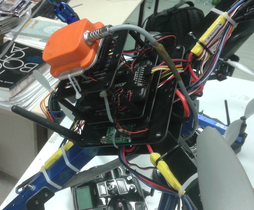
Figure 5: The Inertial Measurements Unit Xsens mounted on the test-bench

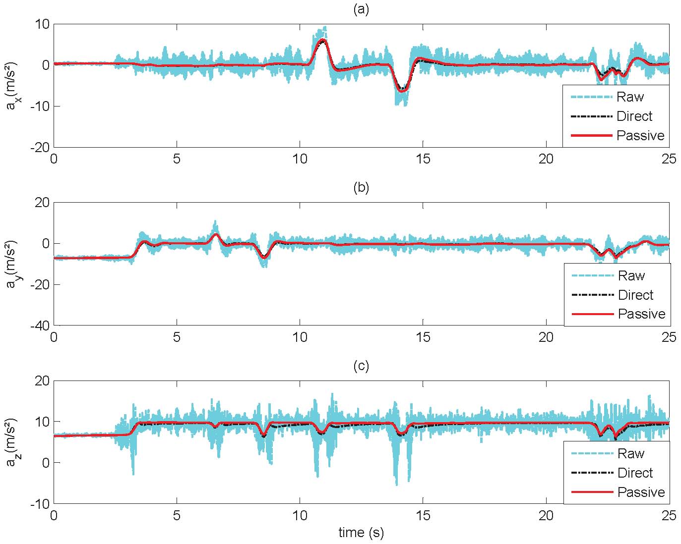
Figure 6: Complementary Accelerometer filters experimental results

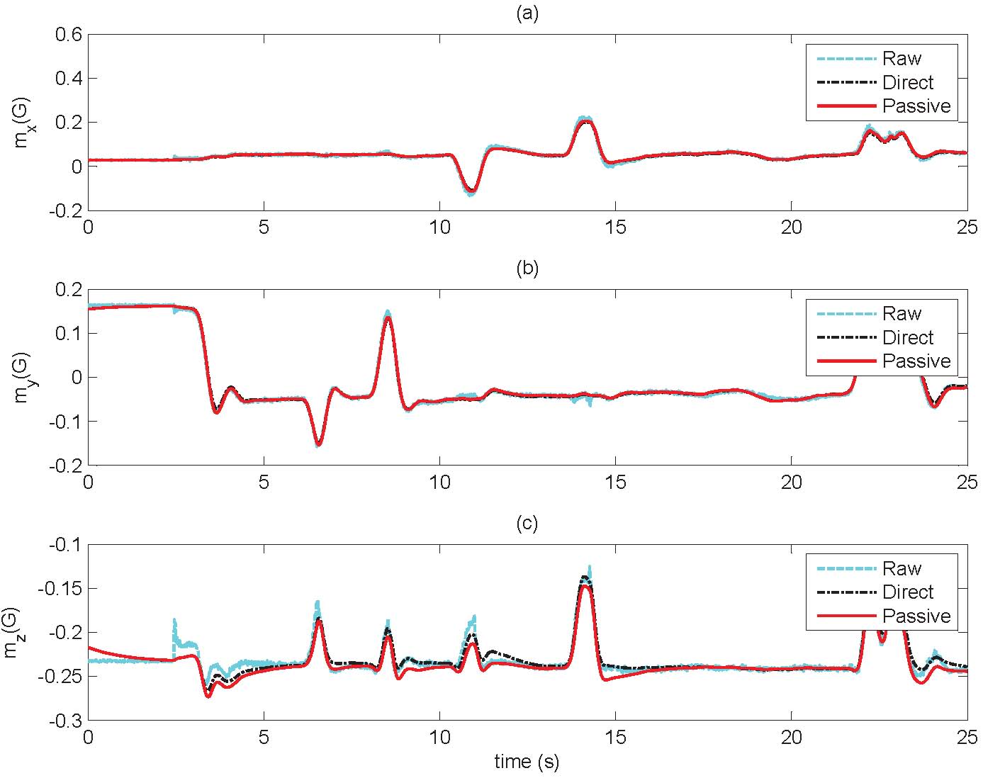
Figure 7: Complementary Magnetometer filters experimental results

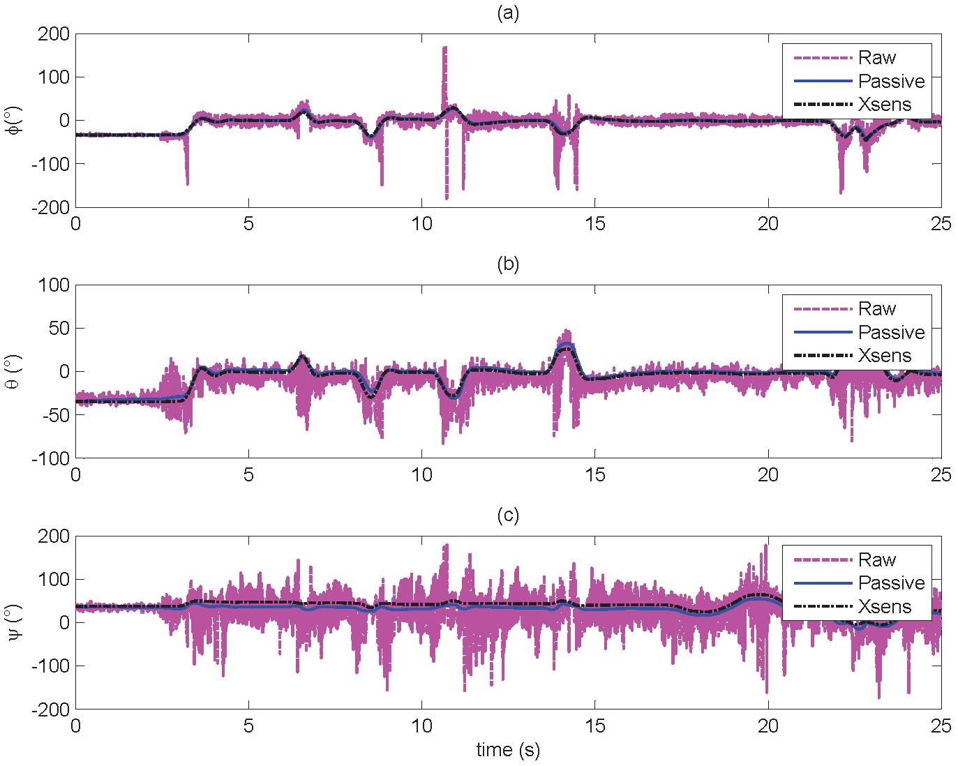
Figure 8: Attitude estimation experimental results for the proposed observers

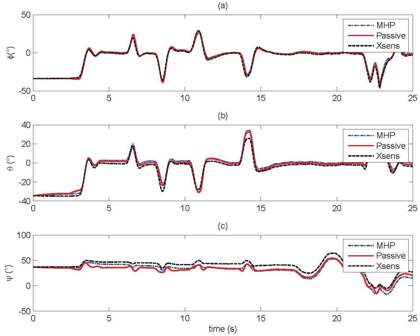
Figure 9: Attitude estimation experimental results comparison

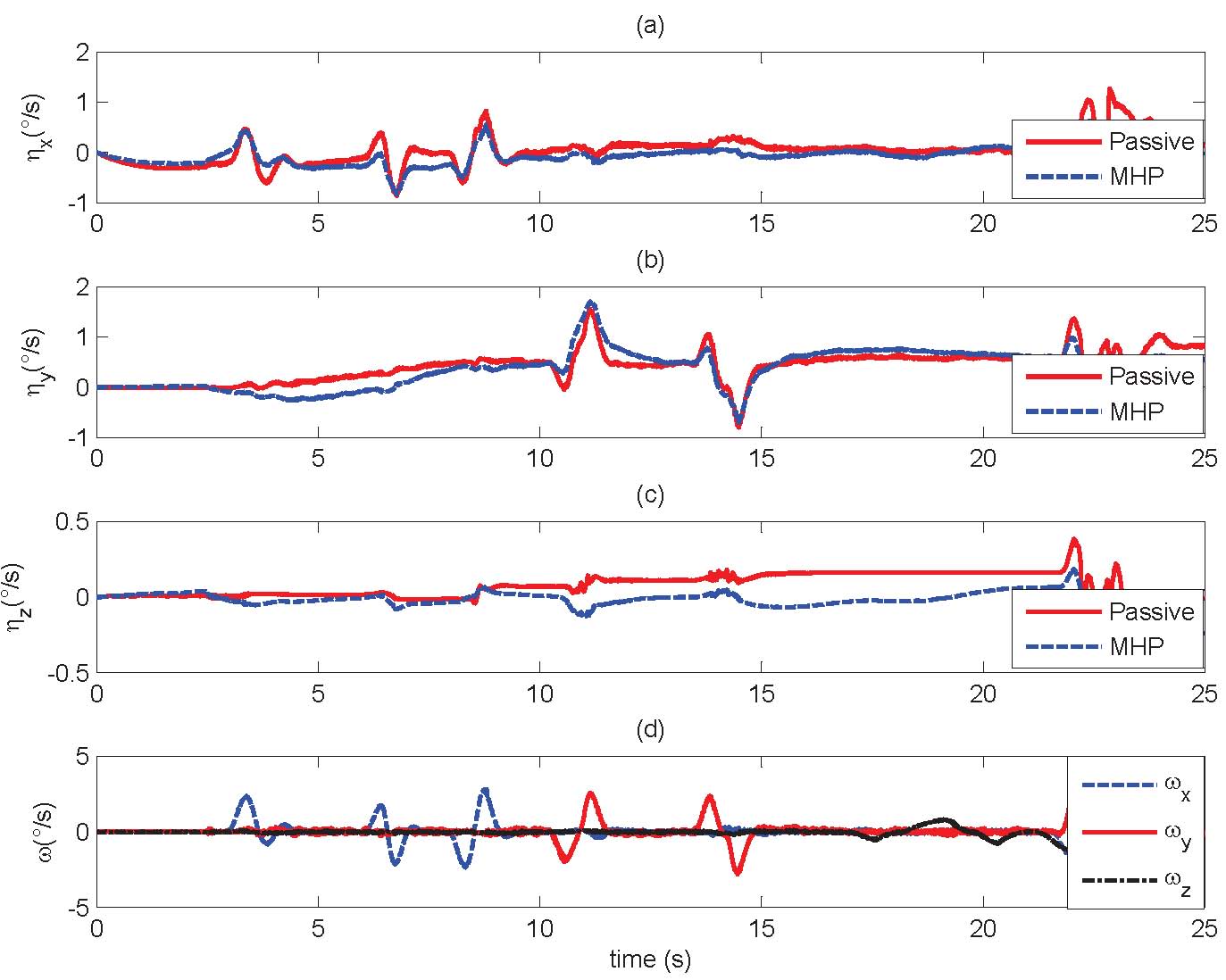
Figure 10: Rate gyro bias estimation experimental results

V-B Attitude stabilization

For this test, we considered for simplicity and without loss of generality the special case of stabilization of attitude. The experiment was done using the test-bench shown in Figure 4. The controller (48) was implemented using the following notations and parameters : $R_{d}(t)=I$, which means $b_{1}^{d}=r_{1}$ and $b_{2}^{d}=r_{2}$; $\hat{b}_{1}=\hat{a}\>(normalized)$, $\hat{b}_{2}=\hat{m}\>(normalized)$ are the estimates of the inertial vector measurements given by the accelerometer and magnetometer, respectively; $\omega(t)\>(rad/s)$ is the rate gyro measurements; $\rho_{1}=1.66$ and $\rho_{2}=0.1161$ (for the axis $x$ and $y$), and $\rho_{1z}=0.05$ and $\rho_{2z}=0.03$ (for the $z$ axis); The damping $k=0.2621$ and the filter gains $\alpha_{1}=6$ and $\alpha_{2}=10$.

The main loop for attitude stabilization is running at 100Hz. At each loop the measurements of accelerometer and magnetometer are normalized after the execution of the observer (41). Due to the poor quality of magnetometer measurements the gains corresponding to $z$ axis are chosen small. Therefore, the stabilization is done around $x$ and $y$ axis only. Then, starting from an arbitrary measured initial condition in Euler angles $(\phi,\theta,\psi)=(-18.478,41.192,2.847)\text{\textdegree}$, the evolution of normalized inertial measurements vectors, torque and Euler angles are shown in Figure 11. We can see that after transient time, the normalized measurements vectors $a$ and $m$ converge to the desired values $b_{1}^{d}=[0,0,1]^{T}$ and $b_{2}^{d}=[0.434,-0.04,0.899]^{T}$. Consequently according with the attitude estimate, this corresponds to the roll and pitch angles close to zero which confirms the stabilization of the platform. We can also observe that control torque is smooth without noise through the use of the complementary filter.

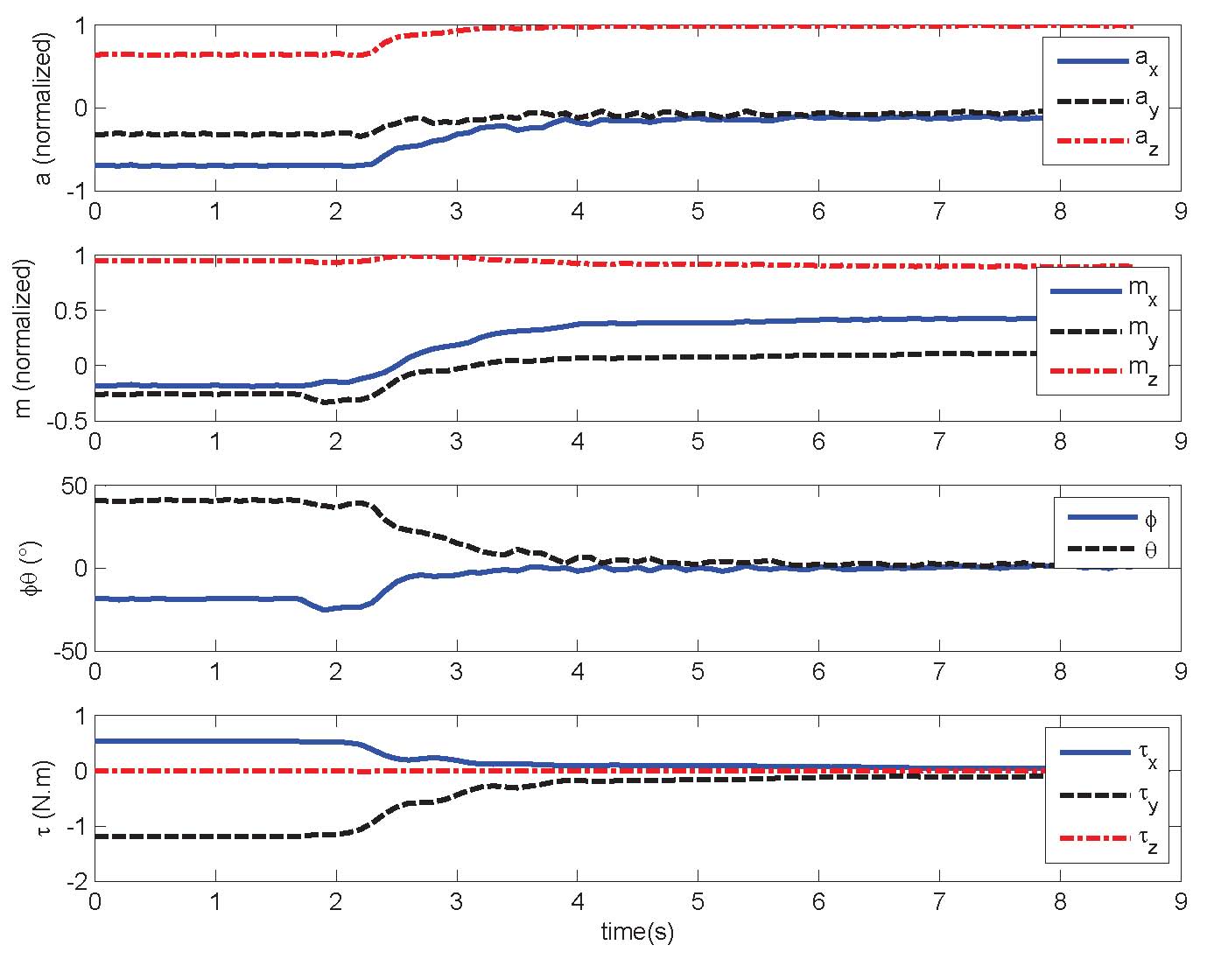
Figure 11: Attitude stabilization experimental results

VI Conclusions

Due to its importance and despite the considerable number of solutions, the problem of attitude estimation and control is still relevant. This paper presents High order “Direct” and “Passive” linear-like complementary filters for attitude and gyro-rate bias estimation. Using Lyapunov analysis, the proposed solutions ensure global convergence. Another novelty of this work lies in the proposition of new control law for attitude tracking problem, in which the principle of data fusion is used. Only filtered inertial vectors and rate gyro measurements were used in the control law, without using “attitude measurements” and ensuring an almost global stability. To show the efficiency and performance of the proposed solutions, a set of experimental tests were performed based on DIY drone Quadcopter, equipped with APM2.6 autopilot. The passive second order filter can be of great help. Indeed, in future work, this filter will be used to enhance the low sampling frequency of magnetometer measurements compared to that of accelerometer.

Proof of Lemma 1

Showing the thesis amounts to exhibit an example. For that purpose, consider $\gamma=(C_{n}^{l}\alpha^{l})_{1\leq l\leq n}\in\mathbb{R}^{n}$, where $n$ is a positive integer, $\alpha$ a positive real number and the $C_{n}^{l}$ are the binomial coefficients. Then $P_{\gamma}(s)=(s+\alpha)^{n}$ implying that $\gamma\in\mathcal{H}_{n}$. It remains to show that $\gamma\in\mathcal{\overline{H}}_{n}$. One clearly has that $P_{\pi(\gamma)}=(P_{\gamma}(s)-P_{\gamma}(0))/s$ and thus the roots of $P_{\pi(\gamma)}$ are the non zero roots of $(s+\alpha)^{n}-\alpha^{n}$. Every root $z$ of the previous polynomial verifies that $(\frac{z}{\alpha}+1)^{n}=1$ and then $\frac{z}{\alpha}+1=e^{j\frac{2k\pi}{n}}$, where $j^{2}=-1$ and $k=0,\ldots,n-1$. It yields that $Re(z)=\alpha(\cos(\frac{2k\pi}{n})-1)$, which is negative only if $k\neq 0$ and in the latter case $z=0$. One deduces that all the roots of $P_{\pi(\gamma)}$ have negative real part, i.e., $P_{\pi(\gamma)}$ is Hurwitz and thus $\gamma\in\mathcal{\overline{H}}_{n}$.

References

• [1] S. Joshi, A. Kelkar, and J.-Y. Wen, “Robust attitude stabilization of spacecraft using nonlinear quaternion feedback,” IEEE Transactions on Automatic Control, vol. 40, no. 10, pp. 1800–1803, 1995.
• [2] J. Thienel and R. Sanner, “A coupled nonlinear spacecraft attitude controller and observer with an unknown constant gyro bias and gyro noise,” IEEE Transactions on Automatic Control, vol. 48, no. 11, pp. 2011–2015, Nov 2003.
• [3] A. Benallegue, A. Mokhtari, and L. Fridman, “High-order sliding-mode observer for a quadrotor uav,” Int. J. Robust and Nonlinear Control, vol. 18, pp. 427–440, 2008.
• [4] A. Tayebi, “Unit quaternion-based output feedback for the attitude tracking problem,” IEEE Transactions on Automatic Control, vol. 53, no. 6, pp. 1516–1520, July 2008.
• [5] T. Lee, “Robust adaptive attitude tracking on so(3) with an application to a quadrotor uav,” IEEE Transactions on Control Systems Technology, vol. 21, no. 5, pp. 1924–1930, 2013.
• [6] D. Thakur and M. R. Akella, “Gyro-free rigid-body attitude stabilization using only vector measurements,” AIAA Journal of Guidance, Control, and Dynamics, pp. 1–8, 2014.
• [7] L. Benziane, A. Benallegue, and A. Tayebi, “Attitude stabilization without angular velocity measurements,” in Proceedings of IEEE International Conference on Robotics & Automation, Hong Kong, China, 2014, pp. 3116–3121.
• [8] A. Tayebi, A. Roberts, and A. Benallegue, “Inertial vector measurements based velocity-free attitude stabilization,” IEEE Transactions on Automatic Control, vol. 58, no. 11, pp. 2893–2898, November 2013.
• [9] G. Wahba, “A least squares estimate of satellite attitude,” SIAM Review, vol. 7, no. 3, p. 409, 1965.
• [10] M. Shuster and S. Oh, “Three-axis attitude determination from vector observations,” Journal of Guidance and Control, vol. 4, no. 1, pp. 70–77, january-february 1981.
• [11] F. L. Markley and D. Mortari, “Quaternion attitude estimation using vector observations.” Journal of the Astronautical Sciences, vol. 48, no. 2, pp. 359–380, 2000.
• [12] J. M. Pflimlina, T. Hamel, and P. Soueres, “Nonlinear attitude and gyroscope’s bias estimation for a vtol uav,” International Journal of Systems Science, vol. 38, pp. 197–210, 2007.
• [13] P. Batista, C. Silvestre, and P. Oliveira, “Partial attitude and rate gyro bias estimation: observability analysis, filter design, and performance evaluation,” International Journal of Control, vol. 84, no. 5, pp. 895–903, Jul 2011.
• [14] J. Crassidis, F. Markley, and F. Cheng, “Survey of nonlinear attitude estimation methods,” Journal of guidance, control, and dynamics, vol. 30, no. 01, pp. 12–28, January 2007.
• [15] M. Jun, S. Roumeliotis, and G. Sukhatme, “State estimation of an autonomous helicopter using kalman filtering,” in Proceedings IEEE/RSJ International Conference on Intelligent Robots and Systems, vol. 3, 1999, pp. 1346 – 1353.
• [16] A. El Hadri and A. Benallegue, “Attitude estimation with gyros-bias compensation using low-cost sensors,” in Joint 48th IEEE Conference on Decision and Control and 28th Chinese Control Conference, Shanghai, P.R. China, December 16-18 2009, pp. 8077–8082.
• [17] J. Crassidis and M. F.L., “Unscented filtering for spacecraft attitude estimation,” Journal of guidance, control, and dynamics, vol. 26, no. 4, pp. 536–542, 2003.
• [18] M. Shuster, “A survey of attitude representations,” The Journal of the astronautical science, vol. 41, no. 4, pp. 439–517, October-December 1993.
• [19] M. Euston, P. Coote, R. Mahony, J. Kim, and T. Hamel, “A complementary filter for attitude estimation of a fixed-wing uav,” in IEEE/RSJ International Conference on Intelligent Robots and Systems, Acropolis Convention Center, Nice, France, Sept, 22-26 2008, pp. 340–345.
• [20] J. Vasconcelos, C. Silvestre, P. Oliveira, P. Batista, and C. B., “Discrete time-varying attitude complementary filter,” in American Control Conference Hyatt Regency Riverfront, St. Louis, MO, USA, June 10-12 2009, pp. 4056–4061.
• [21] J. W. T. Higgins, “A comparison of complementary and kalman filtering,” IEEE Transaction On Aerospace And Electronic Sysytems, vol. AES-1 1, no. 3, pp. 321–325, May 1975.
• [22] P. Martin and E. Salaun, “Design and implementation of a low-cost observer-based attitude and heading reference system,” Control Engineering Practice, vol. 18, no. 7, pp. 712–722, July 2010.
• [23] R. Mahony, T. Hamel, and P. J.-M., “Nonlinear complementary filters on the special orthogonal group,” IEEE Transactions on Automatic Control, vol. 53 , Issue: 5, pp. 1203 – 1218, June 2008.
• [24] A. Tayebi, A. Roberts, and A. Benallegue, “Inertial measurements based dynamic attitude estimation and velocity-free attitude stabilization,” in American Control Conference, San Francisco, CA, USA, June 29 - July 01 2011, pp. 1027–1032.
• [25] V. Kubelka and M. Reinstein, “Complementary filtering approach to orientation estimation using inertial sensors only,” in IEEE International Conference on Robotics and Automation, RiverCentre, Saint Paul, Minnesota, USA, May 14-18 2012, pp. 599–605.
• [26] K. Masuya, T. Sugihara, and M. Yamamoto, “Design of complementary filter for high-fidelity attitude estimation based on sensor dynamics compensation with decoupled properties,” in IEEE International Conference on Robotics and Automation, RiverCentre, Saint Paul, Minnesota, USA, May 14-18 2012, pp. 606–611.
• [27] P. Batista, C. Silvestre, and P. Oliveira, “Sensor-based globally asymptotically stable filters for attitude estimation: Analysis, design, and performance evaluation,” IEEE Transactions on Automatic Control, vol. 57, pp. 2095 – 2100, Aug. 2012.
• [28] M. Shuster, “The triad algorithm as maximum likelihood estimation,” Journal of the Astronautical Sciences, vol. 54, no. 1, pp. 113–123, January-March 2006.
• [29] L. Benziane, A. Benallegue, and A. El-Hadri, “A globally asymptotic attitude estimation using complementary filtering,” in Proceedings of IEEE International Conference on Robotics and Biomimetics, Guangzhou, China, 2012, pp. 878–883.
• [30] 3DR. (2015, Jan) http://copter.ardupilot.com/.
• [31] R. A. Horn and C. R. Johnson, Topics in Matrix Analysis.   Cambridge University Press, 1991.
• [32] L. Benziane, A. Benallegue, Y. Chitour, and A. Tayebi, “Inertial vector based attitude stabilization of rigid body without angular velocity measurements,” arXiv:1501.04767 [math.OC], 2015.
• [33] 3DR. (2015, Jan) http://store.3drobotics.com/. Berkeley, USA.