Calcium H & K and sodium D absorption induced by the interstellar and circumgalactic media of the Milky Way

Abstract

We map out calcium II & sodium I absorption (Fraunhofer H, K & D lines) induced by both the interstellar medium and the circumgalactic medium of the Milky Way. Our measurements cover more than $9000$ deg² and make use of about $300,000$ extragalactic spectra from the Sloan Digital Sky Survey. We present absorption maps for these two species and then compare their distributions to those of neutral hydrogen and dust. We show that the abundance of Na 1 with respect to neutral hydrogen stays roughly constant in different environments, while that of Ca 2 decreases with hydrogen column density. Studying how these tracers vary as a function of velocity, we show that, on average, the $N_{\rm{Na\,I}}$/$N_{\rm{Ca\,II}}$ ratio decreases at higher velocity with respect to the local standard of rest, similar to the local Routly-Spitzer effect but seen on Galactic scale. We show that it is likely caused by higher gas/dust density at lower velocity. Finally, we show that Galactic Ca 2 and Na 1 absorption needs to be taken into account for precision photometry and, more importantly, for photometric redshift estimation with star forming galaxies. Our maps of Ca 2 and Na 1 absorption are publicly available.

1 Introduction

Various advances in our understanding of the Universe have been enabled by sky surveys mapping emission and absorption features across the sky. Historically, William Herschel pioneered this approach by mapping the density of stars and revealing the existence of ”dark holes” (Herschel, 1785), known today as dust clouds. The mapping of globular clusters across the sky allowed Harlow Shapley to infer the disk-like geometry of the Milky Way about one hundred years ago. In the sixties, radio surveys opened up a new window giving us access to the distribution of hydrogen in the Galaxy (e.g., Kalberla & Kerp, 2009). Over the past twenty years, IR observations have provided us with the distribution of dust (e.g., Schlegel et al., 1998) and CO observations that of molecular gas (e.g., Dame et al., 2001). More recently, over the past few years, large-scale maps of diffuse interstellar bands tracing (still unidentified) large molecules have started to emerge (Lan et al., 2014; Zasowski et al., 2015; Baron et al., 2015). Surprisingly, the large-scale distribution of metals in the atomic gas phase – a fundamental component of the ISM – remains poorly measured. Characterizing their spatial distribution is important: while metals are expected to represent about 2% of the mass of the interstellar medium (ISM), they often determine the chemistry, ionization state and temperature of the gas. Their spatial distribution reflects the return to the ISM of gas that has been processed in stars and stellar explosions. As of today, no large-scale map of metals in the gas phase exists.

Gaseous metals can be probed using absorption line spectroscopy. Among the features accessible in the optical window, the Ca 2 and Na 1 lines are the most prominent. They correspond to the H, K and D lines discovered by Fraunhofer in the solar spectrum two hundred years ago (Fraunhofer 1814). Over the last two centuries, these Fraunhofer lines have played an important role in the understanding of a variety of astronomical phenomena both in the Milky Way (e.g., Hartmann, 1904; Routly & Spitzer, 1952) and on extragalactic scales (e.g., Boksenberg & Sargent, 1978; Blades et al., 1981). In this paper we use a large set of extragalactic spectra observed by the Sloan Digital Sky Survey (SDSS, York et al., 2000) to measure the absorption induced by the Milky Way. Interestingly, while such information is encoded in virtually any extragalactic spectrum, no systematic extraction and analysis has been attempted on a large scale. Only Poznanski et al. (2012) measured Na 1 absorption in SDSS galaxy spectra to characterize its cross-correlation with dust reddening. We create maps of Ca 2 and Na 1 absorption over a quarter of the sky induced by gas in and around the Milky Way, i.e., in both the ISM and the circumgalactic medium (CGM), and study their global correlations with other baryonic tracers, such as neutral hydrogen and dust grains. The Ca H & K doublet corresponds to the fine structure splitting of the singly ionized calcium excited states Ca 2 ($\rm{Ca^{+}}$) at $\lambda=3934.78\,$Å (K) & $3969.59\,$Å (H) in vacuum, and Na D, which is also a doublet, corresponds to the fine structure splitting of the neutral sodium excited states at $\lambda=5891.58\,$Å (D₂) & $5897.56\,$Å (D₁) in vacuum. Since their discovery they have played important roles in astrophysics because of their strength and their location in the visible part of the spectrum. Both calcium and sodium are among the most abundant heavy elements, with $\log(\rm{Ca/H})_{\odot}+12\simeq 6.34$ and $\log(\rm{Na/H})_{\odot}+12\simeq 6.24$ (Asplund 2009), and are found in a variety of astrophysical environments. The ionization potentials are $6.11\,$eV, $11.87\,$eV and $50.91\,$eV for Ca 1, Ca 2 and Ca 3, and $5.14\,$eV and $47.29\,$eV for Na 1 and Na 2 (Morton, 2003). With ionization potentials lower than $1$ Rydberg, Ca 2 and Na 1 are therefore not the dominant stage of ionization in most astrophysical environments.

The paper is organized as follows. In Section 2, we briefly describe the data set and method. In Section 3, we present the maps of Ca 2 and Na 1 absorption and investigate the correlations of metal absorption with neutral hydrogen and dust. We discuss the effect of metal absorption on precision photometry in Section 4. Section 5 summarizes our main results.

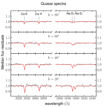
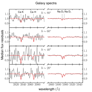
Figure 1: Examples of stacked continuum-normalized residual spectra of quasars (left panel) and galaxies (right panel) in four Galactic latitude bins. The red lines represent the best-fit double-Gaussian profiles.

2 The data

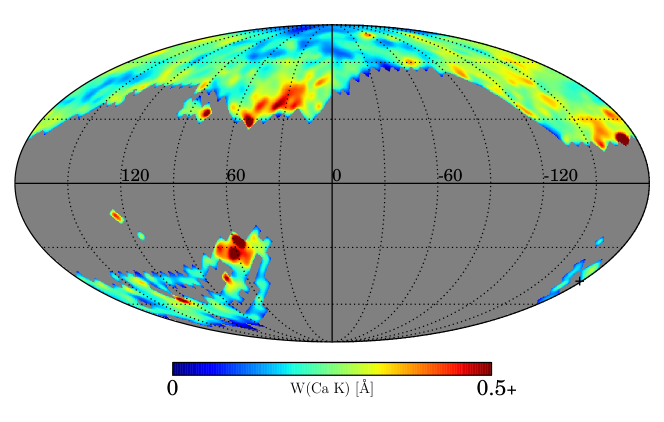
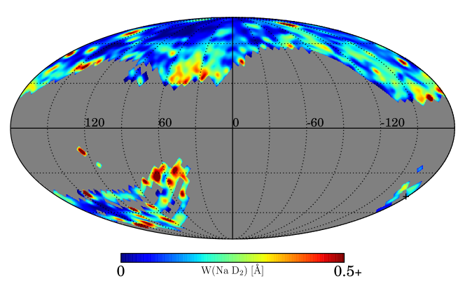
Figure 2: Maps of Ca 2 (top) and Na 1 (bottom) created from measurements of Fraunhofer H and ${\rm D}_{2}$ absorption lines in the spectra of about 300,000 quasars and galaxies from the Sloan Digital Sky Survey. These maps use the Mollweide projection and show the equivalent width of each line from 0 to $0.5\,$Å using a 3-degree Gaussian smoothing. Note that to visually enhance the constrast, equivalent width values greater than $0.5\,$Å are saturated. This affects only a small fraction of the pixels.

We derive our absorption measurements from quasar and galaxy spectra taken from the SDSS Data Release 7 (DR7, Abazajian et al., 2009). For quasars, we use the quasar catalog compiled by Schneider et al. (2010) and the improved redshift estimates given by Hewett & Wild (2010). For galaxies, we use the MPA-JHU value-added catalog (e.g., Tremonti et al., 2004). Absorption line measurements require accurate estimation of the intrinsic background source continuum $\hat{F}(\lambda)$. Below we briefly describe the continuum estimates we use:

• Quasar continuum estimation: We use the estimates provided by Zhu & Ménard (2013a), who used a basis set of quasar eigenspectra created with the dimensionality-reduction technique nonnegative matrix factorization (NMF, Lee & Seung, 1999; Blanton & Roweis, 2007). Large-scale residuals not accounted for by the NMF basis set are removed with appropriate median filters. This set of flux residuals has been used to create a sample of about 50,000 absorber systems (Zhu & Ménard, 2013a), to measure the total amount of Ca 2 around low-redshift galaxies (Zhu & Ménard, 2013b) and Mg 2 around luminous red galaxies at $z\sim 0.5$ (Zhu et al., 2014).

• Galaxy continuum estimation: We use estimates of their intrinsic continumn fluxes provided by Zhu et al. (2010). These authors modeled the observed galaxy spectra using single stellar population (SSP) models of Bruzual & Charlot (2003) with the Padova 1994 library of stellar evolution tracks (e.g., Alongi et al., 1993) and the Chabrier (2003) initial mass function (IMF). For this analysis, we restrict the selection of galaxies to those at redshift $>0.2$, most of which are so-called luminous red galaxies (LRGs) with well-understood spectral energy distribution. Because red galaxies have low-level fluxes blueward of the $4000\,$Å break, there is limited information of Ca 2 absorption induced by the foreground sources, we will use galaxy spectra only for Na 1 absorption.

In total, we make use of spectra of $84,533$ quasars and $181,286$ galaxies. These sources cover about a quarter of the sky, mostly at high Galactic latitude in the northern hemisphere with relatively low dust extinction. We note that all the background sources used here are extragalactic objects and the spectral resolution is $69\,{\rm km~{}s}^{-1}$. All the absorption measurements presented here therefore include contributions from all gas, including both in the ISM and the CGM, of the Milky Way.

To cross-correlate our maps of metal absorption with the distributions of hydrogen and dust we use the following datasets:

• Neutral hydrogen: The Leiden/Argentine/Bonn (LAB) Galactic H 1 Survey Kalberla & Kerp (2009) merged the Leiden/Dwingeloo Survey (LDS: Hartmann & Burton, 1997) in the northern sky and the Instituto Argentino de Radioastronomía Survey (IAR: Arnal et al., 2000; Bajaja et al., 2005) in the south and present an all-sky brightness temperature map of the $21\,{\rm cm}$ hyperfine emission by neutral hydrogen. The LAB Survey is the most sensitive Milky Way H 1 survey to date, with the most extensive coverage both spatially and kinematically. In the optically thin regime, the integrated emission yields total neutral hydrogen column density $N_{\rm{H\,I}}$ in the Milky Way, which we use to compare with our statistical metal absorption measurements. For $N_{\rm{H\,I}}$, we use the values integrated over the full velocity range, from $-450\,{\rm km~{}s}^{-1}$ to $400\,{\rm km~{}s}^{-1}$.

• Dust: Schlegel et al. (1998) derived Galactic reddening $E_{B-V}$ over the full sky from a composite $100\,\mu{\rm m}$ of the COBE/DIRBE (e.g., Boggess et al., 1992) and IRAS/ISSA maps (e.g., Wheelock et al., 1994), assuming uniform dust properties with values of $R_{V}=A_{V}/E_{B-V}\approx 3.1$. We here use $E_{B-V}$ as a proxy of line-of-sight dust column density and adopt their derivations.

For both $N_{\rm{H\,I}}$ and $E_{B-V}$, we use the maps distributed on the NASA LAMBDA website, which were produced under the HEALPix scheme (Górski et al., 2005). The HEALPix pixelization divides a spherical surface into pixels with the same area. The main parameter of the pixelization is the number of pixels along a fixed longitude $N_{\rm side}$. Both $N_{\rm{H\,I}}$ and $E_{B-V}$ maps were stored with $N_{\rm side}=512$, which divides the whole sky into 3,145,728 pixels, with the resolution of approximately $0.01\,$sq. deg per pixel.

3 Analysis

Given the typical signal-to-noise ratio of SDSS quasar and galaxy spectra, the Ca 2 and Na 1 absorption lines induced by the Milky Way are in general not detectable in individual spectra. Their detection requires constructing averaged continuum-normalized residual spectra. To do so we use an inverse-variance weighted estimator, using the wavelength-dependent errors given by the SDSS pipeline. With the stacked residual spectra we then measure the rest equivalent width of the Ca 2 and Na 1 doublets with a double-Gaussian profile, allowing the width and line ratio to be free parameters. In Figure 1, we present examples of stacked spectra as a function of Galactic latitude, showing clear detections of Ca 2 and Na 1 absorption. The best-fit double-Gaussian profiles are presented with the red lines. As shown in the right panel of the Figure, there is limited information about Ca 2 absorption using galaxy spectra. This is because we are using red galaxies which have little fluxes blueward of the $4000\,$Å break. In the following, we therefore use only quasars as background sources for Ca 2, while for Na 1  we combine both quasars and galaxies as a whole sample.

3.1 Absorption Maps

Figure 3: Rest equivalent width of Ca 2 K (top panel) and Na 1 D₂ (middle panel) as a function of Galactic latitude $b$. The errorbars represent $1\sigma$ errors from the double-Gaussian fitting. For comparison, in the bottom panel we show the average neutral hydrogen column density $N_{\rm{H\,I}}$ in the same footprint, using values from the LAB H 1 survey. The errorbars for $N_{\rm{H\,I}}$ are $1\sigma$ dispersion in the pixels used.

To create maps of Ca 2 and Na 1 absorption we pixelize the sky using the HEALPix scheme. We choose the number of pixels along the Galactic longitude to be $N_{\rm side}=16$, which divides the whole sphere into $3072$ pixels with equal area of about $3.7^{\circ}\times 3.7^{\circ}$. This choice of resolution is motivated by the surface number density of objects so that in the majority of the pixels, we have enough objects for a signal-dominated determination of the absorption strength. In total, our data cover about $700$ pixels (about $9,100\,{\rm deg}^{2}$), and we have on average about $120$ quasars and $270$ galaxies in a pixel. For each of these resolution elements we perform a double-Gaussian fitting to the stacked residual spectra and measure the rest equivalent width of each line. At that resolution, the typical S/N with which such lines are detected is about $3$.

Figure 2 presents maps of Ca 2 K and Na 1 D₂ absorption in the Mollweide projection. They show the equivalent width of each line from 0 to $0.5\,$Å using a 3-degree Gaussian smoothing. Note that to visually enhance the constrast, equivalent width values greater than $0.5\,$Å are saturated. This affects only a small fraction of the pixels. Both maps show large-scale gradients as a function of Galactic latitude. The distribution of Na 1 appears to be more concentrated towards the disk of the Milky Way. To characterize this dependence, we measure the mean absorption strength as a function of latitude, using only data from the Northen Galactic hemisphere where the coverage is more complete. We present the mean equivalent width of Ca 2 and Na 1 measured in bins with $\Delta b=10^{\circ}$ in Figure 3, where the errorbars show the $1\sigma$ dispersion of all the pixels. For comparison, we also show the average H 1 column density in the bottom panel, where $N_{\rm{H\,I}}$ is the median value over all pixels of the $N_{\rm{H\,I}}$ HEALPix map in each latitude bin within the same SDSS footprint. Both the Ca 2 and Na 1 absorption, and $N_{\rm{H\,I}}$ decrease from low latitude towards high latitude. This is likely due to a combination of longer path through the disk at low latitude and higher local column density in the ISM.

3.2 Correlations with Neutral Hydrogen and Dust

More information on the distributions of Ca 2 and Na 1 can be extracted from these maps using cross-correlations with other tracers. This allows one to make use of signal lying below the noise level of individual HEALPix pixels. In this section we present measurements of cross-correlations with the observed distributions of Galactic neutral hydrogen and dust. We note here that previous attempts to measure correlations between metal absorption, hydrogen and dust were typically based on datasets targetting “dense” clouds. By using spectra of extragalactic sources and integrating the absorption signal over a large number of lines-of-sight, our approach allows us to probe the total amount of absorption originating from both dense clouds as well as the diffuse interstellar and circumgalactic media. So far, only one such approach has been used: Poznanski et al. (2012) performed a similar statistical study of Ca 2 absorption.

To investigate the dependence of Ca 2 and Na 1 absorption on $N_{\rm{H\,I}}$ and $E_{B-V}$, we use the high-resolution HEALPix maps of $N_{\rm{H\,I}}$ and $E_{B-V}$ distributed by the LAMBDA website. We divide all the HEALPix pixels into bins with $\Delta\log_{10}N_{\rm{H\,I}}=0.05$ and $\Delta\log_{10}E_{B-V}=0.05$. We then find all objects (quasars and galaxies for Na 1, quasars for Ca 2) in the corresponding pixels, construct stacked continuum-normalized residual spectra and measure the equivalent width of Ca 2 and Na 1. Note that we do not spatially downgrade the $N_{\rm{H\,I}}$ and $E_{B-V}$ HEALPix maps (with $N_{\rm side}=512$) but instead we select objects in pixels with the same $N_{\rm{H\,I}}$ or $E_{B-V}$ values. In Figure 4, we present the correlations of the rest equivalent width of Ca 2 and Na 1 as a function of $N_{\rm{H\,I}}$ and $E_{B-V}$, where the errorbars are from the double-Gaussian fitting. Both Ca 2 and Na 1 absorption strengths correlate strongly with $N_{\rm{H\,I}}$ and $E_{B-V}$, increasing linearly towards higher density until saturation effect becomes important at $N_{\rm{H\,I}}$$\sim 5\times 10^{20}\,{\rm cm}^{-2}$ and $E_{B-V}$$\sim 0.08\,$mag. However the observed correlations indicate that the environmental dependence of Na 1 and Ca 2 abundance are different. Poznanski et al. (2012) performed a similar correlation analysis between Na 1 and $E_{B-V}$ and obtained similar results.

Parameters	Ca K	Ca H	Na D2	Na D1
$N_{0}/10^{21}$ ($N_{\rm H\,I}$)	13.18$\pm$ 4.92	32.53$\pm$ 10.83	2.08$\pm$ 0.24	2.36$\pm$ 0.18
$\alpha_{0}$ ($N_{\rm H\,I}$)	0.35$\pm$ 0.03	0.39 $\pm$ 0.03	0.77 $\pm$ 0.04	1.01 $\pm$ 0.04
$E_{0}$ ($E_{B-V}$)	4.21 $\pm$ 2.46	10.90 $\pm$ 7.47	0.39 $\pm$ 0.09	0.26 $\pm$ 0.02
$\beta_{0}$ ($E_{B-V}$)	0.29 $\pm$ 0.03	0.33 $\pm$ 0.04	0.63 $\pm$ 0.05	1.06 $\pm$ 0.04

Table 1: Best-fit parameters for the ${\rm W}_{0}$-$N_{\rm{H\,I}}$/$E_{B-V}$ relations (Equation 1 and 2).

We characterize the trends by the following relations:

$$W(N_{\rm H\,I})=\left(\frac{N_{\rm H\,I}}{N_{0}}\right)^{\alpha_{0}}\;{\rm\AA}\ \mathrm{,}$$ (1)

and

$$W(E_{B-V})=\left(\frac{E_{B-V}}{E_{0}}\right)^{\beta_{0}}\;{\rm\AA}\ \mathrm{.}$$ (2)

We estimate the best fit parameters considering only the range where $N_{\rm{H\,I}}$$<5\times 10^{20}\,{\rm cm}^{-2}$ and $E_{B-V}$$<0.08$. Above these values the observed trends indicate that the absorption lines become saturated. The best-fit parameters are presented in Table 1 and the corresponding trends are overplotted with dash lines in Figure 4. Equations 1 and 2 provide us with a way to estimate the average absorption strength of Ca 2 and Na 1 at a given $N_{\rm{H\,I}}$ and $E_{B-V}$. It is interesting to note that the slope of $W_{0}^{\rm Na\,I}$-$N_{\rm{H\,I}}$ (and $E_{B-V}$) relation is close to unity, while the slope of $W_{0}^{\rm Ca\,II}$-$N_{\rm{H\,I}}$ is shallower with a best-fit value of about $0.4$. The weaker dependence of the Ca 2 absorption on $N_{\rm{H\,I}}$ could be due to either the lower dust depletion level of calcium or higher ionization parameter or both in lower-density environments. We further investigate the abundances of Ca 2 and Na 1 and their dependence on $N_{\rm{H\,I}}$ in the next section.

3.2.1 Abundance of Ca 2 and Na 1

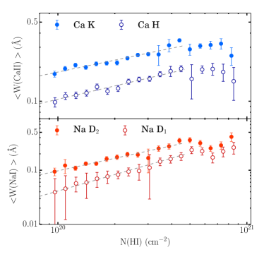
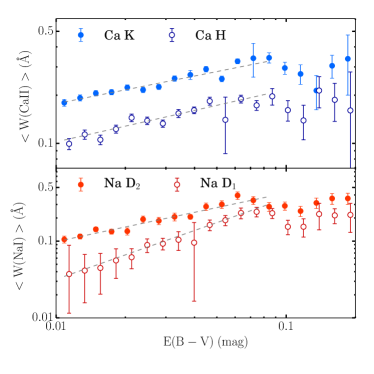
Figure 4: The dependence of Ca 2 and Na 1 absorption on neutral hydrogen column density ($N_{\rm{H\,I}}$, left panel) and Galactic reddening ($E_{B-V}$, right panel). The lines represent the best-fit linear relations with data at $N_{\rm H\,I}<5\times 10^{20}\,{\rm cm}^{-2}$ and $E_{B-V}<0.08\,$mag.

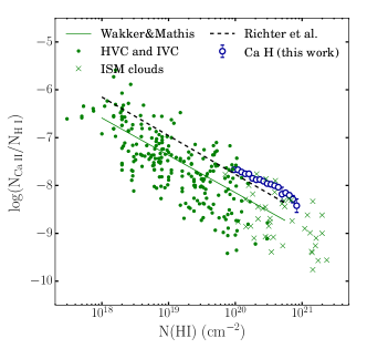
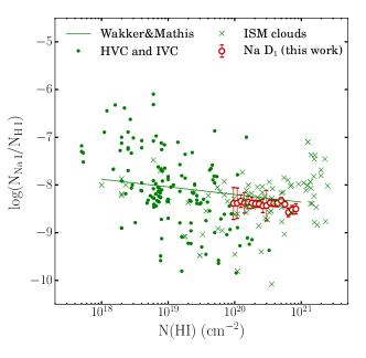
Figure 5: The dependence of Na 1 and Ca 2 abundance on neutral hydrogen $N_{\rm{H\,I}}$. The open circles represent the measurements in our statistical analysis, integrated over the full velocity range. The dots and crosses show the abundances of individual systems, HVC/IVC and ISM clouds, from high-resolution spectroscopy, compiled by Wakker & Mathis (2000). The solid lines are their best-fit linear relations to these individual systems. The dashed line in the left panel shows the best-fit relation to extragalactic Ca 2 absorbers by Richter et al. (2011).

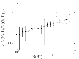
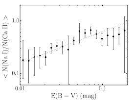
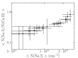
Figure 6: The dependence of the $N_{\rm{Na\,I}}$/$N_{\rm{Ca\,II}}$ ratio on $N_{\rm{H\,I}}$, $E_{B-V}$ and $N_{\rm{Na\,I}}$.

We now investigate the dependence of Ca 2 and Na 1 abundances on hydrogen column density. We first estimate the Ca 2 and Na 1 column density using the weaker line of each doublet under the assumption of negligible saturation. Using the linear curve-of-growth relation at low column density, we convert the rest equivalent width of the weaker lines ($W_{0}^{\rm D_{1}}$ and $W_{0}^{\rm H}$) to column density and calculate the relative abundance $N_{\rm Ca\,II}/N_{\rm H\,I}$ and $N_{\rm Na\,I}/N_{\rm H\,I}$. When the absorption is in the linear regime of the curve of growth, the rest equivalent width is related to the column density with

$$N=1.13\times 10^{20}~{}\mathrm{cm}^{-2}~{}\frac{W_{0}}{f\lambda^{2}}\,\mathrm{,}$$ (3)

where both $W_{0}$ and $\lambda$ are in unit of Å and the oscillator strength $f$ for the Ca 2 H line is $0.324$ (Safronova & Safronova, 2011) and for Na 1 $\mathrm{D}_{1}$ is $0.320$ (Kelleher & Podobedova, 2008). This relation is valid when the optical depth is smaller than unity, which corresponds to $N_{\rm Ca\,II,Na\,I}<\sim 10^{12.5}\,{\rm cm}^{-2}$ (assuming the Doppler broadening factor $b\sim 10\,{\rm km~{}s}^{-1}$). The measurements are presented in Figure 5 with open circles. The Na 1 abundance is roughly constant within the $N_{\rm{H\,I}}$ range probed, while the Ca 2 abundance decreases rapidly with increasing $N_{\rm{H\,I}}$.

Our measurements are integrated values over the full velocity range with contributions from both the ISM in the disk and the CGM in the halo. To better understand the physics of the correlations, we compare our measurements with a compilation of abundances of individual systems based on high-resolution spectroscopy (Wakker & Mathis, 2000). In Figure 5, the cross symbols represent the measurements of abundance in the ISM clouds, the dotted symbols show the measurements of abundance in high-velocity clouds (HVCs) and intermediate-velocity clouds (IVCs), and the solid lines are the best-fit linear relations by Wakker & Mathis (2000) for these individual systems. In the left panel, we also overplot the best-fit relation by Richter et al. (2011) who studied the abundance of Ca 2 of about ten extragalactic absorber systems. Our measurements of the average Na 1 abundance at a given total $N_{\rm{H\,I}}$ coincide with the abundance of individual systems, while the average Ca 2 abundance is closer to the relation of extragalactic systems and overall about half a dex higher than those of ISM clouds, though with a similar dependence on $N_{\rm{H\,I}}$.

We would like to stress that the variables in our analysis, the neutral hydrogen column density ($N_{\rm{H\,I}}$), the metal absorption strength and column density, are all integrated values over the full velocity range. The neutral hydrogen column density is dominated by the contribution from the ISM, because along a given line of sight the contribution from the ISM is orders-of-magnitude higher than from the CGM, even if the sightline covers an HVC or IVC. The Na 1 abundance of individual systems, though with a large scatter, on average is roughly constant at different densities. The integrated Na 1 absorption in our analysis therefore must also be dominated by the contribution from the ISM and this explains why the average Na 1 abundance is consistent with that of the individual systems. The Ca 2 abundance of individual systems, on the other hand, is orders-of-magnitude higher at low density than at high density. Zhu & Ménard (2013b) show that the total amount of Ca 2 in the CGM, averaged over all galaxies, is about an order-of-magnitude larger than that in the ISM of the Milky Way (see also Richter et al., 2011). In our analysis, making use of extragalactic sources, Ca 2 column densities are therefore expected to carry a significant CGM contribution, while hydrogen column densities are mostly originating from the Milky Way disk. We thus expect our measurements to display average values of Ca 2 abundance that are higher than those obtained for individual clouds, as shown in figure 5.

In Figure 6, we further investigate the dependence of the relative abundance of Na 1 and Ca 2 ($N_{\rm{Na\,I}}$/$N_{\rm{Ca\,II}}$) on $N_{\rm{H\,I}}$, $E_{B-V}$ and $N_{\rm{Na\,I}}$. The $N_{\rm{Na\,I}}$/$N_{\rm{Ca\,II}}$ ratio is higher at higher hydrogen/dust/Na 1 density, increasing from about $0.4$ at $N_{\rm H\,I}\sim 10^{20}\,{\rm cm}^{-2}$ ($E_{B-V}\sim 0.01\,{\rm mag}$) to $2$ at $N_{\rm H\,I}\sim 10^{21}\,{\rm cm}^{-2}$ ($E_{B-V}\sim 0.1\,{\rm mag}$). We fit these relations with similar power-law functions as in Figure 4:

$$N_{\rm Na\,I}/N_{\rm Ca\,II}=\left(\frac{N_{\rm H\,I}}{N_{1}}\right)^{\alpha_{1}}\ \mathrm{,}$$ (4)

and

$$N_{\rm Na\,I}/N_{\rm Ca\,II}=\left(\frac{E_{B-V}}{E_{1}}\right)^{\beta_{1}}\ \mathrm{,}$$ (5)

and

$$N_{\rm Na\,I}/N_{\rm Ca\,II}=\left(\frac{N_{\rm Na\,I}}{N_{2}}\right)^{\alpha_{2}}\ \mathrm{.}$$ (6)

The best-fit relations are given in Table 2 and overplotted in Figure 6. The slopes are both positive, indicating that the $N_{\rm{Na\,I}}$/$N_{\rm{Ca\,II}}$ ratio is higher in denser environments.

Parameters	$N_{{\rm Na\,I}}/N_{{\rm Ca\,II}}$
$N_{1}/10^{21}$ ($N_{\rm H\,I}$)	2.13$\pm$ 0.40
$\alpha_{1}$ ($N_{\rm H\,I}$)	0.53$\pm$ 0.04
$E_{1}$ ($E_{B-V}$)	0.22 $\pm$ 0.06
$\beta_{1}$ ($E_{B-V}$)	0.60 $\pm$ 0.07
$N_{2}/10^{12}$ ($N_{\rm Na\,I}$)	7.07$\pm$ 0.82
$\alpha_{2}$ ($N_{\rm Na\,I}$)	0.58$\pm$ 0.03

Table 2: Best-fit parameters for the $N_{\rm{Na\,I}}$/$N_{\rm{Ca\,II}}$ ratio-$N_{\rm{H\,I}}$/$E_{B-V}$/$N_{\rm{Na\,I}}$ relations (Equation 4, 5 and 6).

This environmental dependence of the $N_{\rm{Na\,I}}$/$N_{\rm{Ca\,II}}$ ratio has been noticed for decades (e.g., Phillips et al., 1984; Vallerga et al., 1993; Ben Bekhti et al., 2012). However, the physical reason is yet to be determined. It is generally attributed to the different dust depletion levels of sodium and calcium at different densities, but other factors such as ionization effects can yield the same dependence. We here briefly discuss two theories.

A possible scenario was proposed by Phillips et al. (1984, see also ): During the formation of dust grains, sodium is not highly depleted to begin with because of relatively high condensation temperature and low absorbing energy, so density does not play a role in its low depletion level. On the other hand, calcium can be easily accreted onto surface of dust grains due to relatively low condensation temperature and high absorbing energy. At higher density, its accretion rate is higher yet the destruction rate is lower because of greater UV shielding and enhanced mantle growth, while at lower density, calcium trapped in grain surface is easier to be ejected by shock sputtering. All these dynamic processes result in higher calcium depletion level at higher density.

When an analysis is sensitive to both ISM and CGM absorption, it is important to take into account of the environmental dependence of metallicity and dust abundance. Gas clouds in the CGM, such as HVCs and the Magellanic Stream, have lower metallicity (about $0.1\,$solar, see Wakker et al., 1999; Richter et al., 2001; Fox et al., 2013) and dust-to-gas ratio (Lu et al., 1998) than those in the ISM. Although the total abundance of Ca and Na is lower in the CGM due to lower metallicity, the overall dust depletion level is also lower because of the low dust content. The combined effects of these dependences therefore can result in the observed dependence of the $N_{\rm{Na\,I}}$/$N_{\rm{Ca\,II}}$ ratio on the environment.

Another theory is based on that the ionization parameter is higher at lower density, and neither Ca 2 nor Na 1 is the dominant ionization state. Models with density-dependent ionization parameters but constant dust depletion level can reproduce the dependence of the $N_{\rm{Na\,I}}$/$N_{\rm{Ca\,II}}$ ratio on environment . The exact mechanism responsible for this density dependence of Ca 2 and Na 1 abundances is still an open question.

3.3 The Routly-Spitzer effect measured on large scales

Routly & Spitzer (1952) found that the average $N_{\rm{Na\,I}}$/$N_{\rm{Ca\,II}}$ ratio decreases when the cloud velocity $|v_{\rm LSR}|$ (measured in the local standard of rest) increases. This so-called Routly-Spitzer effect is usually derived from measurements of individual systems in the local ISM within tens of kilometer per second (Vallerga et al., 1993). Recently, Ben Bekhti et al. (2012) reported a similar effect for individual absorption systems, based on deviation velocity measurements in the halo of the Milky Way, extending the detection of the Routly-Spitzer effect to larger scales. Here we investigate if such an effect also exists in our statistical data.

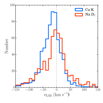
Figure 7: The velocity distributions of Ca 2 and Na 1 absorption in the local standard of rest using measurements from the northern Galactic hemisphere. The distribution for Ca 2 is offset from the origin and wider than that of Na 1. This is consistent with the interpretation that Na 1 originates mostly from the disk while Ca 2 also traces a significant amount of material from the circumgalactic medium.

To study the dependence of the $N_{\rm{Na\,I}}$/$N_{\rm{Ca\,II}}$ ratio on $v_{\rm LSR}$, we use the HEALPix maps as presented in Figure 2. In each HEALPix pixel, we determine the centroid wavelength from the double-Gaussian fitting and calculate the velocity offset from the rest-frame wavelength of the doublets. When doing so we find that Na 1 and Ca 2 are on average blueshifted by $8$ and $23\,{\rm km~{}s}^{-1}$ in the heliocentric reference frame. We then convert these observed velocities to the local standard of rest (LSR, Courteau & van den Bergh, 1999). We show the corresponding distributions of absorption velocities for Ca 2 and Na 1 in the northern hemisphere in Figure 7. As can be seen, Ca 2 tends to be found at lower velocities compared to Na 1. We find the mean of the Na 1 velocity distribution to be about $-3\,{\rm km~{}s}^{-1}$, while the value for Ca 2 is found to be about $-17\,{\rm km~{}s}^{-1}$. Recent H 1 surveys have shown that, in the northern sky, the high- and intermediate-velocity clouds have on average negative velocities (Richter et al., 2003; Putman et al., 2012). The higher detection rate of Ca 2 at negative velocities is therefore consistent with the interpretation that Ca 2 detected in the extragalactic sources traces a significant amount of gas from the CGM.

We then group the pixels with similar $v_{\rm LSR}^{\rm Na\,I}$ values and measure the mean $W_{0}^{\rm Na\,I}$ and $W_{0}^{\rm Ca\,II}$ in each $v_{\rm LSR}^{\rm Na\,I}$ bin. We note that using the velocity derived from Ca 2 produces similar trends with a larger scatter. The left panel of Figure 8 shows our measurements of the $N_{\rm{Na\,I}}$/$N_{\rm{Ca\,II}}$ ratio as a function of $v_{\rm LSR}^{\rm Na\,I}$. Interestingly, we find that the average $N_{\rm{Na\,I}}$/$N_{\rm{Ca\,II}}$ ratio shows a similar dependence on $v_{\rm LSR}$ as the local Routly-Spitzer effect for individual systems, therefore our data show that the velocity dependence of $N_{\rm{Na\,I}}$/$N_{\rm{Ca\,II}}$ ratio also exists on the Galactic scale. Barlow & Silk (1977) suggested that it is related to dust destruction. One of the major mechanisms of dust destruction is sputtering by interstellar shocks. The destruction rate depends on the shock velocity which results in higher dust destruction rate and higher Ca 2 abundance relative to Na 1 at higher velocity. Subsequent theoretical analyses and simulations have lent support to such proposition (e.g., Draine & Salpeter, 1979; McKee, 1989; Jones et al., 1994). However, it is also possible that this effect can be just a consequence of the density dependence of the $N_{\rm{Na\,I}}$/$N_{\rm{Ca\,II}}$ ratio shown in the previous section, regardless of the actual cause. In the middle and right panels of Figure 8, we show that the Na 1 density has a similar dependence on $v_{\rm LSR}$ as the $N_{\rm{Na\,I}}$/$N_{\rm{Ca\,II}}$ ratio, while Ca 2 density has a much weaker dependence. Since the $N_{\rm{Na\,I}}$/$N_{\rm{Ca\,II}}$ ratio is higher in higher-density environment, as probed by Na 1, H 1 and dust (Figure 6), this can therefore explain part of the velocity dependence. The mechanisms responsible for the Routly-Spitzer effect on large scales can therefore be more complicated than interstellar shock only.

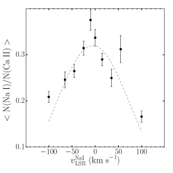
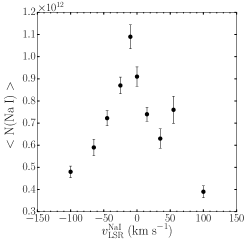
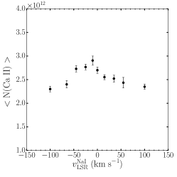
Figure 8: The global Routly-Spitzer effect. The left panel shows the dependence of the $N_{\rm{Na\,I}}$/$N_{\rm{Ca\,II}}$ ratio on $v_{\rm LSR}$ of Na 1. The right panels show $N_{\rm{Na\,I}}$ and $N_{\rm{Ca\,II}}$ as a function of $v_{\rm LSR}$. Note the y-axis ranges in the right two panels are consistent, i.e., the maximum is a factor of four of the minimum in both cases.

4 Implications for photometric observations and redshift estimation

The Ca 2 $\lambda\lambda 3934,3969$ and Na 1 $\lambda\lambda 5890,5896$ absorption lines due to the ISM and CGM of the Milky Way are expected to impact the broad band photometry of extragalactic objects. Two types of effects can occur:

• absorption on top of continuum flux: Metal line absorption is expected to suppress a fraction of the expected flux from extragalactic sources. This effect has been statistically detected in the broad band photometry of distant quasars Ménard & Fukugita (2012). We note that the distribution of metals in the gas phase does not exactly track that of the dust. Therefore infrared emission (as used in SFD) cannot be used to precisely map this kind of absorption.

• Absorption at the location of emission lines: if a redshifted emission line happens to coincide with one of the Galactic absorption features, the apparent broad-band color of the corresponding galaxy can be appreciably modified. This can happen when, for example, [O 3] $\lambda 5007$ is seen on top of Na D at $z\sim 0.176$ or [O 2] $\lambda 3727$ is seen on top of Na D at $z\sim 0.58$. This introduces a level of degeneracy between redshift and color for star forming galaxies and is expected to impact the accuracy of photometric redshift estimation (see Rahman et al. (in prep) for a more extended discussion of this effect).

5 Summary

The light emitted by extragalactic sources has to penetrate the ubiquitous gas and dust in the interstellar and circum-galactic media of the Milky Way. Every extragalactic spectrum therefore carries information about these two environments.

We have used the large collection of quasar and galaxy spectra obtained by the Sloan Digital Sky Survey to detect absorption lines induced by the presence of Ca 2 and Na 1. The absorption signal is typically too weak to be detected in individual SDSS spectra. Measuring it requires a statistical approach. Not until recently had this avenue been explored (e.g., Poznanski et al., 2012; Lan et al., 2014; Zasowski et al., 2015; Baron et al., 2015). We have created maps revealing the spatial distribution of Ca 2 and Na 1 absorption on the sky. We have then used these new datasets to study correlations between these two components and other baryonic tracers. Our analysis has allowed us to obtain the following results:

• We have mapped out the Na 1 D and Ca 2 H & K absorption over about a quarter of the sky, obtaining signal-dominated measurements at a resolution of about one degree. The corresponding maps are publicly available.

• Cross-correlating these absorption maps with H 1 column density and dust reddening maps, we find that the dependence of Ca 2 absorption on $N_{\rm{H\,I}}$ and $E_{B-V}$ is much weaker than Na 1and provide fitting formulae for the average relations between these quantities. We find the abundance of Na 1 with respect to neutral hydrogen to be roughly constant in different environments, while the Ca 2 abundance decreases with hydrogen column density. We discuss the possible mechanisms that can cause such different behaviors, including dust depletion and ionization effects.

• We show that, on average, the $N_{\rm{Na\,I}}$/$N_{\rm{Ca\,II}}$ ratio decreases with velocity with respect to the local standard of rest up to velocities reaching $100\,{\rm km~{}s}^{-1}$. Interestingly, this is consistent with the local Routly-Spitzer effect originally measured for individual systems within a much smaller velocity range.

• We commented on the fact that Galactic absorption lines can change the apparent colors of emission line galaxies at specific redshifts, which can possibly impact photometric redshift estimation.

The detection of absorption features relies on the ability to accurately estimate the intrinsic spectral energy distribution of the background source. To do so we have used the continuum estimates of quasars presented in Zhu & Ménard (2013a), based on a vector-decomposition method, and of galaxies by Zhu et al. (2010), based on stellar spectral templates. Our work demonstrates that large spectroscopic surveys, though designed for studies of the light sources themselves or cosmology, provide valuable datasets for studies of the ISM and CGM of our own Milky Way. We have only just started to explore this avenue and there is more information to be extracted. For example, the absorption induced in the spectra of extragalactic sources includes contributions from both the ISM and CGM of the Milky Way, while absorption in the stellar spectra only has contribution from the ISM up to the star’s distance, differential analysis therefore can be performed to produce a 3D map of the gas distribution in and around the Milky Way. The continuum-estimation methods and statistical absorption-line spectroscopic approaches we developed are robust, generic, and readily applicable to any large datasets from ongoing and future surveys, such as SDSS-IV, DESi and PFS.

References

- Abazajian et al. (2009) Abazajian, K. N., Adelman-McCarthy, J. K., Agüeros, M. A., et al. 2009, ApJS, 182, 543
- Alongi et al. (1993) Alongi, M., Bertelli, G., Bressan, A., et al. 1993, A&AS, 97, 851
- Arnal et al. (2000) Arnal, E. M., Bajaja, E., Larrarte, J. J., Morras, R., Pöppel, W. G. L. 2000, A&AS, 142, 35
- Asplund et al. (2009) Asplund, M., Grevesse, N., Sauval, A. J., & Scott, P. 2009, ARA&A, 47, 481
- Bajaja et al. (2005) Bajaja, E., Arnal, E. M., Larrarte, J. J., Morras, R., Pöppel, W. G. L., Kalberla, P. M. W. 2005, A&A, 440, 767
- Barlow (1978) Barlow, M. J. 1978, MNRAS, 183, 417
- Barlow & Silk (1977) Barlow, M. J., & Silk, J. 1977, ApJ, 211, L83
- Baron et al. (2015) Baron, D., Poznanski, D., Watson, D., Yao, Y., & Prochaska, J. X. 2015, MNRAS, 447, 545
- Ben Bekhti et al. (2012) Ben Bekhti, N., Winkel, B., Richter, P., et al. 2012, A&A, 542, A110
- Blades et al. (1981) Blades, J. C., Hunstead, R. W., & Murdoch, H. S. 1981, MNRAS, 194, 669
- Blanton & Roweis (2007) Blanton, M. R., & Roweis, S. 2007, AJ, 133, 734
- Blitz et al. (1999) Blitz, L., Spergel, D. N., Teuben, P. J., Hartmann, D. and Burton, W. B. 1999, ApJ, 514, 818
- Boggess et al. (1992) Boggess, N. W., Mather, J. C., Weiss, R., Bennett, C. L., Cheng, E. S., Dwek, E., Gulkis, S., Hauser, M. G., Janssen, M. A., Kelsall, T., Meyer, S. S., et al. 1992, ApJ, 397, 420
- Boksenberg & Sargent (1978) Boksenberg, A., & Sargent, W. L. W. 1978, ApJ, 220, 42
- Bruzual & Charlot (2003) Bruzual, G., & Charlot, S. 2003, MNRAS, 344, 1000
- Chabrier (2003) Chabrier, G. 2003, PASP, 115, 763
- Courteau & van den Bergh (1999) Courteau, S. and van den Bergh, S. 1999, AJ, 118, 337
- Dame et al. (2001) Dame, T. M., Hartmann, D., & Thaddeus, P. 2001, ApJ, 547, 792
- Draine & Salpeter (1979) Draine, B. T. and Salpeter, E. E. 1979, ApJ, 231, 438
- Fox et al. (2013) Fox, A. J., Richter, P., Wakker, B. P., et al. 2013, ApJ, 772, 110
- Fraunhofer (1814) Fraunhofer, J. 1814, Denkschriften der Kˆniglichen Akademie der Wissenschaften zu München, 5, 193
- Górski et al. (2005) Górski, K. M., Hivon, E., Banday, A. J., Wandelt, B. D., Hansen, F. K., Reinecke, M., Bartelmann, M. 2005, ApJ, 622, 759
- Hartmann (1904) Hartmann, J. 1904, ApJ, 19, 268
- Hartmann & Burton (1997) Hartmann, D., Burton, W. B. 1997, Atlas of Galactic Neutral Hydrogen (Cambridge University Press), ISBN 0521471117
- Herschell (1785) Herschell, W., “On the Construction of the Heavens,” Philosophical Transactions of the Royal Society of London, 75, 213-266 (1785).
- Hewett & Wild (2010) Hewett, P. C., & Wild, V. 2010, MNRAS, 405, 2302
- Jones et al. (1994) Jones, A. P., Tielens, A. G. G. M., Hollenbach, D. J., & McKee, C. F. 1994, ApJ, 433, 797
- Kalberla & Kerp (2009) Kalberla, P. M. W., & Kerp, J. 2009, ARA&A, 47, 27
- Kelleher & Podobedova (2008) Kelleher, D. E., & Podobedova, L. I. 2008, Journal of Physical and Chemical Reference Data, 37, 267
- Kupka et al. (2000) Kupka, F. G., Ryabchikova, T. A., Piskunov, N. E., Stempels, H. C., Weiss, W. W., Baltic astronomy, 9, 590
- Lan et al. (2014) Lan, T.-W., Ménard, B., & Zhu, G. 2014, arXiv:1406.7284
- Land & Slosar (2007) Land, K. and Slosar, A. 2007, Phys. Rev. D, 76, 087301
- Lee & Seung (1999) Lee, D. D., & Seung, H. S. 1999, Nature, 401, 788
- Lu et al. (1998) Lu, L., Sargent, W. L. W., Savage, B. D., et al. 1998, AJ, 115, 162
- McKee (1989) McKee, C. F. 1989, ApJ, 345, 782
- Ménard & Fukugita (2012) Ménard, B. and Fukugita, M. 2012, ApJ, 754, 116
- Morton (2003) Morton, D. C. 2003, ApJS, 149, 205
- Phillips et al. (1984) Phillips, A. P., Pettini, M., & Gondhalekar, P. M. 1984, MNRAS, 206, 337
- Poznanski et al. (2012) Poznanski, D., Prochaska, J. X., & Bloom, J. S. 2012, MNRAS, 426, 1465
- Putman et al. (2012) Putman, M. E., Peek, J. E. G., & Joung, M. R. 2012, ARA&A, 50, 491
- Richter et al. (2011) Richter, P., Krause, F., Fechner, C., Charlton, J. C., & Murphy, M. T. 2011, A&A, 528, A12
- Richter et al. (2003) Richter, P., Wakker, B. P., Savage, B. D., & Sembach, K. R. 2003, ApJ, 586, 230
- Richter et al. (2001) Richter, P., Sembach, K. R., Wakker, B. P., et al. 2001, ApJ, 559, 318
- Routly & Spitzer (1952) Routly, P. M., & Spitzer, Jr., L. 1952, ApJ, 115, 227
- Safronova & Safronova (2011) Safronova, M. S., & Safronova, U. I. 2011, Phys. Rev. A, 83, 012503
- Savage & Sembach (1996) Savage, B. D., & Sembach, K. R. 1996, ARA&A, 34, 279
- Schlegel et al. (1998) Schlegel, D. J., Finkbeiner, D. P., & Davis, M. 1998, ApJ, 500, 525
- Schneider et al. (2010) Schneider, D. P., Richards, G. T., Hall, P. B., et al. 2010, AJ, 139, 2360
- Tremonti et al. (2004) Tremonti, C. A., et al. 2004, ApJ, 613, 898
- Vallerga et al. (1993) Vallerga, J. V., Vedder, P. W., Craig, N. and Welsh, B. Y. 1993, ApJ, 411, 729
- Wakker (1991) Wakker, B. P. 1991, A&A, 250, 499
- Wakker & Mathis (2000) Wakker, B. P., & Mathis, J. S. 2000, ApJ, 544, L107
- Wakker et al. (1999) Wakker, B. P., Howk, J. C., Savage, B. D., et al. 1999, Nature, 402, 388
- Wheelock et al. (1994) Wheelock, S. L., Gautier, T. N., Chillemi, J., Kester, D., McCallon, H., Oken, C., White, J., etc. 1994, NASA STI/Recon Technical Report N, 95, 22539
- York et al. (2000) York, D. G., Adelman, J., Anderson, J. E., Jr., et al. 2000, AJ, 120, 1579
- Zasowski et al. (2015) Zasowski, G., Ménard, B., Bizyaev, D., et al. 2015, ApJ, 798, 35
- Zhu et al. (2010) Zhu, G., Blanton, M. R., & Moustakas, J. 2010, ApJ, 722, 491
- Zhu & Ménard (2013a) Zhu, G., & Ménard, B. 2013a, ApJ, 770, 130
- Zhu & Ménard (2013b) —. 2013b, ApJ, 773, 16
- Zhu et al. (2014) Zhu, G., Ménard, B., Bizyaev, D., et al. 2014, MNRAS, 439, 3139