Entanglement over the rainbow

Abstract

In one dimension the area law for the entanglement entropy is violated maximally by the ground state of a strong inhomogeneous spin chain, the so called concentric singlet phase (CSP), that looks like a rainbow connecting the two halves of the chain. In this paper we show that, in the weak inhomogeneity limit, the rainbow state is a thermofield double of a conformal field theory with a temperature proportional to the inhomogeneity parameter. This result suggests some relation of the CSP with black holes. Finally, we propose an extension of the model to higher dimensions.

I Introduction

Entanglement has become a very useful tool to study the structure of complex quantum states, such as the ground states (GS) of interacting systems Amico.RMP.08 . Geometry and quantum structure are linked via the so-called area laws Sredniki.PRL.93 ; Eisert.RMP.10 , which state that the entanglement entropy of a block $B$, calculated in the ground state of a local Hamiltonian, scales with the area of the boundary of the block. Area laws have been proved only in a few cases, such as 1D gapped systems Hastings.JSTAT.07 , and are violated in several interesting cases, such as conformal systems in 1D Holzhey.NPB.94 ; Vidal.PRL.03 ; Calabrese.JSTAT.04 , where the entropy grows logarithmically with the block size, with a prefactor proportional to the central charge of the conformal field theory (CFT). These exceptions of the area law have received an increasing attention in recent studies Hujse_Swingle.PRB.13 ; Trombettoni.14 .

A strong violation of the area law takes place in an inhomogeneous free fermion model in 1D where the hopping amplitudes between consecutive sites decay exponentially outwards from the center of the chain Vitagliano.NJP.10 . By tuning the exponential factor, the GS of the system evolves smoothly from a logarithmic law towards a volume law for the entanglement entropy between the left and the right halves of the chain Ramirez.rainbow.14 . In the strong inhomogeneity regime, when the exponential factor is high enough, the GS is the product state of Bell-pairs symmetrically distributed around the center of the system, as shown in Fig. 1. This valence bond state was termed concentric singlet phase (CSP) Vitagliano.NJP.10 or simply, rainbow state Ramirez.rainbow.14 . The volume law for strong inhomogeneous chains can be easily understood from the rainbow picture. The entanglement entropy of half of the chain is given essentially by the number of bonds connecting the left and the right halves. However, for weak inhomogeneities the rainbow picture does not hold because the GS is a resonating valence bond state that satisfies a volume law plus logarithmic corrections Ramirez.rainbow.14 . Another type of inhomogeneity has been used to provide smooth boundary conditions which improve the convergence of the bulk properties of the GS Vekic.93 . Moreover, an exponential increase of the couplings has been used in a Kondo-like problem Okunishi.10 and a hyperbolic increase for the study of the scaling properties of non-deformed systems Ueda.09 ; Ueda.10 .

The aim of this paper is to understand the free fermion model in the weak inhomogeneity regime and its relation to the uniform limit given by a conformal field theory, namely a massless Dirac fermion with open boundary conditions. One might think that some scaling limit of the model would correspond to a perturbation of the underlying CFT. However, the perturbation cannot correspond to local operators added to the action, since they do not give rise to volume law entropies. Quite surprisingly, the solution of this puzzle is still provided by CFT: the GS is a sort of thermal state that satisfies a volume law, with a temperature related to the exponential factor of the hopping amplitudes. From this perspective, the appearance of a volume law in the GS of the model is not surprising at all since, after all, it corresponds to a thermal state. Yet, it comes as a surprise that the state remains pure. The understanding of this apparent contradiction will bring us to unexpected territories that we shall start to explore.

The organization of the paper is as follows. After a general reminder of our model in section II, containing an analysis of the strong inhomogeneity limit, we establish in section III a continuum approximation in the vicinity of the homogeneous point, given by a deformation of the critical Hamiltonian. This deformation affects the single-particle wavefunctions and the low-energy excitations. In section IV, we study the entanglement entropy within the CSP. The continuum approximation of the previous section allows us to give an expression for the von Neumann and Rényi entropies of the left half of the system throughout the transition. Moreover, we show how the Rényi block entropies fit to the conformal expressions with varying coefficients. In section V we address the question: can the maximal area-law violation of the deformed hopping Hamiltonian be extended to higher dimensions? Indeed, we find that a natural extension of the concentric singlet phase can be found in 2D systems. The article ends with a summary of our conclusions and ideas for further work. Finally, in appendix A, qubistic images Laguna.NJP.12 are shown to provide useful information about the entanglement structure.

II Model and Notation

II.1 Strong Disorder Renormalization of the Hopping Model

Let us consider a strongly inhomogeneous XX-model

$$H_{XX}=\sum_{i=1}^{L-1}K_{i}(\sigma^{x}_{i}\sigma^{x}_{i+1}+\sigma^{y}_{i}\sigma^{y}_{i+1}),$$ (1)

where the $K_{i}>0$ are very different in value. We can apply the strong disorder renormalization group (SDRG) of Ma and Dasgupta Ma.PRB.80 in order to obtain the GS. The renormalization prescription is to pick up the strongest coupling, $K_{max}$, and to establish a singlet bond on top of it. Then, using second order perturbation theory, one finds the effective coupling between the two neighbours of the singlet,

$$\tilde{K}={K_{L}K_{R}\over K_{max}},$$ (2)

where $K_{L}$ and $K_{R}$ are, respectively, the left and right couplings to the maximal one. The renormalization continues by choosing the next largest coupling and so on. Effective couplings may therefore emerge at long distances. The success of the SDRG scheme depends on the maximal coupling $K_{max}$ being always much larger than its neighboring values $K_{L}$ and $K_{R}$.

Using the Jordan-Wigner transformation, we can apply the same tools to study a fermionic hopping model in 1D with the same features Ramirez.rxx.14 ; Ramirez.rainbow.14 , reading the couplings $K_{i}$ as hopping amplitudes, $J_{i}$:

$$H=\sum_{i=1}^{L-1}J_{i}c^{\dagger}_{i}c_{i+1}+\mathrm{h.c.}\,,$$ (3)

where $c^{\dagger}_{i}$ creates a spinless fermion on site $i$, and is related to $\sigma^{+}_{i}$ via the non-local Jordan-Wigner transformation:

$$c^{\dagger}_{i}=\sigma^{+}_{i}\prod_{j=1}^{i-1}\sigma^{z}_{j}\,.$$ (4)

This non-local transformation points at a modification of the SDRG prescription to take into account the fermionic nature of the particles. Effective hoppings between non-contiguous sites are equal to the corresponding coupling in the XX model multiplied by a sign, $J=(-1)^{n_{F}}K$, where $n_{F}$ is the number of fermions between the two sites footnote1 . This rule can be implemented with a simple modification of the renormalization group (RG) prescription. Since a single fermion is always added at each RG step,

$$\tilde{J}=-{J_{L}J_{R}\over J_{max}}\,.$$ (5)

This implies that the hoppings can be either positive or negative. When they are positive, a singlet-type bond is established between both sites, of the form $|\Psi^{-}\rangle\propto|01\rangle-|10\rangle$. If the hopping is negative, the corresponding triplet-type anti-bond is established: $|\Psi^{+}\rangle\propto|01\rangle+|10\rangle$. Both types of bonds share many properties, such as the entanglement. They both represent different flavors of a Bell pair. The SDRG candidate for the GS of the system is a tensor product of bond or anti-bond states on the corresponding sites. Indeed, it can be written as a Fermi state:

$$|GS\rangle=\prod_{k=1}^{L/2}d^{\dagger}_{k}|0\rangle,$$ (6)

where $d^{\dagger}_{k}$ creates either a bond or an anti-bond on a pair of sites, i.e.: $d^{\dagger}_{k}\propto c^{\dagger}_{i}\pm c^{\dagger}_{j}$.

It was proved in Ramirez.rxx.14 , that the Hamiltonian (3) has the following properties, for any values of the $\{J_{i}\}$. It presents particle-hole symmetry, which implies that for every single-particle eigenstate with energy $\epsilon$ there is another eigenstate with energy $-\epsilon$, which is related by swapping the sign of the components of all odd sites. Thus, the ground state takes place at half-filling. Moreover, the occupation number of every site is equal: $\langle n_{i}\rangle=1/2$. This is a non-intuitive result, given the inhomogeneity of Hamiltonian (1), and it does not hold for excited states.

II.2 The Rainbow State

Let us describe the family of local Hamiltonians whose ground state approaches asymptotically the concentric singlet phase, also known as rainbow state, and give some heuristic arguments to explain the volume law for the entanglement entropy.

Let us consider a chain with $2L$ sites, which we will label using half-odd integers, $n=\pm\frac{1}{2},\pm\frac{3}{2},\cdots,\pm\left(L-\frac{1}{2}\right)$. On each site $n$, let $c_{n}$ and $c^{\dagger}_{n}$ denote the annihilation and creation operators of a spinless fermion. The hopping Hamiltonian is given by footnote2

$$H\equiv-\frac{J_{0}}{2}c_{\frac{1}{2}}^{\dagger}c_{-\frac{1}{2}}-\sum_{n=\frac{1}{2}}^{L-\frac{3}{2}}\frac{J_{n}}{2}\left[c^{\dagger}_{n}c_{n+1}+c^{\dagger}_{-n}c_{-(n+1)}\right]+\mathrm{h.c.}\,,$$ (7)

where $J_{n}$ are the hopping amplitudes parametrized as (see Fig. 1 for an illustration)

$$\left\{\begin{array}[]{lcrl}J_{0}(\alpha)&=&1,&\\ J_{n}(\alpha)&=&\alpha^{2n},&n=\frac{1}{2},\dots,L-\frac{3}{2}.\end{array}\right.$$ (8)

For $\alpha=1$, this is the uniform 1D spinless fermion model with open boundary conditions (OBC). The model with $0<\alpha<1$ was introduced by Vitagliano and coworkers to illustrate a violation of the area law for local Hamiltonians Vitagliano.NJP.10 and was studied in much more detail in reference Ramirez.rainbow.14 .

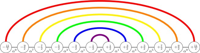
Figure 1: Rainbow state showing the $(-k,+k)$ bonds above the central link. Thus, the entanglement entropy between the left and the right halves of the chain is $L\log 2$.

In the $\alpha\to 0^{+}$ limit, the couplings become strongly inhomogeneous and, as argued in Ramirez.rainbow.14 , we can employ the SDRG described in the previous section. The largest hopping is the central one, $J_{0}=1$, and gets renormalized to $\tilde{J}_{0}=-\alpha^{2}$, larger (in absolute value) than $\alpha^{3}$, which comes next. The values of $J_{n}$ are engineered so that this situation repeats itself for all steps of SDRG, so the bonds are established in a concentric way around the center, joining sites $+k$ and $-k$, and giving rise to the aforementioned CSP, as in Fig. 1. Moreover, notice that the signs alternate.

It is worth to notice the striking similarity between our system and the Kondo chain Wilson.75 . Indeed, let us divide our inhomogeneous chain into three parts: central link, left sites and right sites. The left and right sites correspond, in our analogy, to the spin up and down chains used in Wilson’s chain representation of the Kondo problem. In both cases, they form a system of free fermions, with exponentially decaying couplings. In the Kondo chain, notwithstanding, the central link becomes a magnetic impurity, which renders the full system non-gaussian.

II.3 Strong Inhomogeneity Limit

The $\alpha\to 0^{+}$ limit of (7), leading to the rainbow state, is singular: the Hamiltonian decouples in that limit, and only the central link survives. Let us consider a very small but non-zero $\alpha$, and study the GS to first order in perturbation theory. The Hamiltonian is always free, so the GS is a Slater determinant (6). The orbital operators, $d^{\dagger}_{k}$, can be expanded in terms of the local creation operators:

$$d^{\dagger}_{k}=\sum_{i}\psi^{k}_{i}c^{\dagger}_{i},$$ (9)

where $\psi^{k}_{i}$ are the wavefunction components for the single-body associated problem, i.e., eigenvectors of the hopping matrix. Let us propose the following form for them:

$$\matrix{&&\cdots&-\frac{5}{2}&-\frac{3}{2}&-\frac{1}{2}&+\frac{1}{2}&+\frac{3}{2}&+\frac{5}{2}&\cdots\cr\psi^{1}&=&\cdots&\cdots&\alpha&1&1&\alpha&\cdots&\cdots\cr\psi^{2}&=&\cdots&\alpha&1&\alpha&-\alpha&-1&-\alpha&\cdots\cr\psi^{3}&=&\alpha&1&\alpha&0&0&\alpha&1&\alpha\cr}$$ (10)

Notice the sign alternation, due to the negative sign in the renormalization prescription (5). It is straightforward to check that all those $\psi^{k}$ are eigenstates of the hopping matrix to first order in $\alpha$. We can now define two families of states: the bonding and the anti-bonding creating operators, defined as:

$$\left(b^{+}_{ij}\right)^{\dagger} = {1\over\sqrt{2}}\left(c^{\dagger}_{i}+c^{\dagger}_{j}\right),$$

$$\left(b^{-}_{ij}\right)^{\dagger} = {1\over\sqrt{2}}\left(c^{\dagger}_{i}-c^{\dagger}_{j}\right).$$ (11)

In the limit $\alpha\to 0^{+}$, the GS of Hamiltonian (7) can be written as the concentric singlet state or rainbow state:

$$|R_{L}\rangle\equiv\left(b^{s_{L}}_{-L+\frac{1}{2},L-\frac{1}{2}}\right)^{\dagger}\cdots\left(b^{+}_{-\frac{5}{2},\frac{5}{2}}\right)^{\dagger}\left(b^{-}_{-\frac{3}{2},\frac{3}{2}}\right)^{\dagger}\left(b^{+}_{-\frac{1}{2},\frac{1}{2}}\right)^{\dagger}|0\rangle.$$ (12)

where $s_{L}=(-1)^{L}$.

III Weak Inhomogeneity Limit: Continuum Approximation

The study of the weak inhomogeneity limit, $\alpha\to 1^{-}$, motivates the derivation of a continuum approximation of the Hamiltonian (7). This is obtained by expanding the local operator $c_{n}$ into the slow modes, $\psi_{R}(x)$ and $\psi_{L}(x)$ around the Fermi points $\pm k_{F}$

$$\frac{c_{n}}{\sqrt{a}}\simeq e^{ik_{F}x}\psi_{L}(x)+e^{-ik_{F}x}\psi_{R}(x),$$ (13)

located at the position $x=an\in(-{\cal L},{\cal L})$, where $a$ is the lattice spacing and ${\cal L}=aL$. In the continuum limit, $a\rightarrow 0$ and $L\rightarrow\infty$, with ${\cal L}$ kept constant. At half-filling, $k_{F}=\pi/(2a)$ is the Fermi momentum.

Equation (13) is the familiar expansion used in the uniform case, $\alpha=1$, that will enable us to derive the numerical results found in Ramirez.rainbow.14 . Plugging Eq. (13) into Eq. (7) one obtains

$$H\simeq\frac{ia}{2}\int_{-\cal L}^{\cal L}dx\,e^{-\frac{h|x|}{a}}\left[\psi^{\dagger}_{R}\partial_{x}\psi_{R}-(\partial_{x}\psi^{\dagger}_{R})\psi_{R}-\psi^{\dagger}_{L}\partial_{x}\psi_{L}\right.+\left.(\partial_{x}\psi^{\dagger}_{L})\psi_{L}\right],$$ (14)

where

$$\alpha=e^{-h/2}.$$ (15)

To derive equation (14), we have assumed that the fields $\psi_{R,L}(x)$ vary slowly with $x$, so that cross terms like $(-1)^{x/a}\psi_{R}^{\dagger}(x)\psi_{L}(x)$ can be dropped. We have also made a gradient expansion $\psi(x+a)\simeq\psi(x)+a\partial_{x}\psi(x)$, keeping only terms up to the first derivative. The Hamiltonian (14) describes the low energy excitations of the original lattice Hamiltonian at half-filling. It is worth to mention that (14) is a Hermitian operator, that is, $H^{\dagger}=H$, which is of course a consequence of the hermiticity of (7). In the continuum limit we shall take $h\rightarrow 0$, with $h/a$ kept constant, so that $\alpha\rightarrow 1^{-}$.

The boundary conditions (BC) satisfied by the fields $\psi_{L,R}(x)$ at $x=\pm{\cal L}$, can be derived from equation (13) setting $c_{\pm(L+\frac{1}{2})}=0$ and taking a continuum limit that yields

$$\psi_{R}(\pm{\cal L})=\mp i\,\psi_{L}(\pm{\cal L}).$$ (16)

Then, integrating by parts, one can write Hamiltonian (14) as

$$H\simeq ia\int_{-\cal L}^{\cal L}dx\,e^{-\frac{h|x|}{a}}\left[\psi^{\dagger}_{R}\partial_{x}\psi_{R}-\psi^{\dagger}_{L}\partial_{x}\psi_{L}\right.-\left.\frac{h}{2a}\mathrm{sign(x)}(\psi^{\dagger}_{R}\psi_{R}-\psi^{\dagger}_{L}\psi_{L})\right].$$ (17)

The Fermi velocity is then given by $v_{F}=a$, that we set equal to one by convention (similarly, we replace $h/a\rightarrow h$). The single-body spectrum of the uniform model, that is, $h=0$, can be easily found

$$E_{m}=\frac{\pi(m+1/2)}{2L},\quad m=0,\pm 1,\ldots$$ (18)

For the non-uniform model we have the Eqs.

$$ie^{-h|x|}\left[\partial_{x}\mp\frac{h}{2}\,\mathrm{sign(x)}\right]\psi_{R,L}(x)\quad=\quad\pm E\psi_{R,L}(x),$$ (19)

whose solution is

$$\psi_{R,L}(x)=A_{R,L}e^{h|x|/2}\exp{\left[\mp\frac{iE}{h}\mathrm{sign(x)}\left(e^{h|x|}-1\right)\right]}.$$ (20)

Notice that, in the limit $h\to 0$, one recovers the usual plane-wave solutions $\psi_{R,L}\rightarrow A_{R,L}e^{\mp iEx}$. The BC (16) imply:

$$A_{R}\,\exp{\left[-\frac{iE}{h}\left(e^{hL}-1\right)\right]} = -i\,A_{L}\,\exp{\left[\frac{iE}{h}\left(e^{hL}-1\right)\right]},$$

$$A_{R}\,\exp{\left[\frac{iE}{h}\left(e^{hL}-1\right)\right]} = \quad i\,A_{L}\,\exp{\left[-\frac{iE}{h}\left(e^{hL}-1\right)\right]}.$$ (21)

which, eliminating $A_{R,L}$, yields

$$\exp{\left[\frac{4iE}{h}\left(e^{hL}-1\right)\right]}=-1.$$ (22)

The eigenmodes are then given by

$$E_{m}=\frac{h\pi(m+1/2)}{2(e^{hL}-1)}=a(z)\frac{\pi(m+1/2)}{2L},\quad m=0,\pm 1,\dots$$ (23)

where $a(z)$, defined as

$$a(z)=\frac{z}{e^{z}-1},\qquad z\equiv hL.$$ (24)

was interpreted in reference Ramirez.rainbow.14 as the Fermi velocity. Notice that $z$ has a finite value in the continuum limit since it can be written as $z=(h/a){\cal L}$. In the latter reference it was shown that the single-particle spectrum of the Hamiltonian (7) corresponds to Eq. (23) with a function $a(z)$ given numerically in Fig. 2. As we can see, the analytic expression (24) footnote3 gives a very good fit of the numerical data.

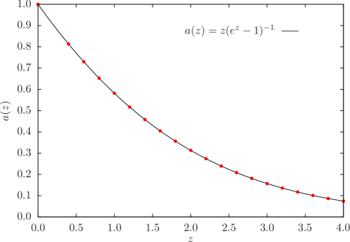
Figure 2: The scaling function $a(z)$ that gives the spectrum of the Hamiltonian (7) near the Fermi energy. The points are the numerical data, i.e., the slope of the spectrum at the Fermi point, and the continuous line is the analytic result.

To find the eigenfunctions with energy $E_{m}$, we first compute the constants $A_{R,L}$ using (21)

$$A_{R,L}=\exp\left\{\pm i\left[\frac{E_{m}}{h}\left(e^{hL}-1\right)-\frac{\pi}{4}\right]\right\},$$ (25)

and Eq. (13), obtaining

$$\psi_{n}^{(m)}\simeq e^{h|n|/2}\cos\left[\frac{\pi(n-m)}{2}+\mathrm{sign(n)}\frac{\pi(m+1/2)}{2}\frac{e^{h|n|}-1}{e^{hL}-1}\right],$$ (26)

where $n=\pm\frac{1}{2},\cdots,\pm\left(L-\frac{1}{2}\right)$ and $m=0,\pm 1,\cdots$. Fig. 3 shows the numerical and analytic values of $\psi_{n}^{(m)}$ for $m=0,1$ and $z=1$ and $2$. As $hn=zn/L$, we see that for the same value of $z$, all the curves collapse when expressed in the scaled variable $n/L$.

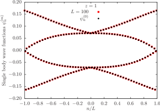
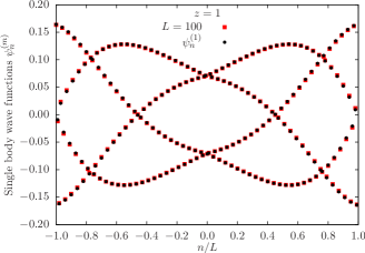
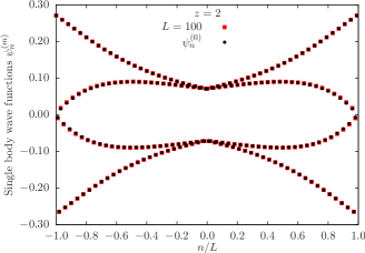
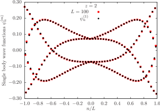
Figure 3: Wavefunctions just below the Fermi level ($m=0$, left column) and the next below the Fermi level ($m=1$, right column) for $z=1$ (top) and $2$ (bottom). The analytic values of $\psi^{(m)}_{n}$ are given by Eq. (26).

The results obtained so far suggest that the continuum Hamiltonian (17) can be brought to the standard canonical form of a free fermion with OBC. To show that this is indeed the case, let us make the change of variables

$$\tilde{x}=\mathrm{sign(x)}\frac{e^{h|x|}-1}{h},$$ (27)

that maps the interval $x\in[-L,L]$ into the interval $\tilde{x}\in[-\tilde{L},\tilde{L}]$ where

$$\tilde{L}=\frac{e^{hL}-1}{h}.$$ (28)

The fermion fields in the variable $\tilde{x}$ are given by

$$\tilde{\psi}_{R,L}(\tilde{x})=\left(\frac{d\tilde{x}}{dx}\right)^{-1/2}\psi_{R,L}(x)=e^{-h|x|/2}\psi_{R,L}(x),$$ (29)

that plugged into (17) gives (recall that we set $a=1$, so ${\cal L}=L$)

$$H\simeq i\int_{-\tilde{L}}^{\tilde{L}}d\tilde{x}\,\left[\tilde{\psi}^{\dagger}_{R}\partial_{\tilde{x}}\tilde{\psi}_{R}-\tilde{\psi}^{\dagger}_{L}\partial_{\tilde{x}}\tilde{\psi}_{L}\right].$$ (30)

That is just the free fermion Hamiltonian for a chain of length $2\tilde{L}$. This result suggests that one could try to derive some of the properties of the rainbow Hamiltonian, Eq. (7), from those of the free fermion system. This will be done in the next section when discussing the entanglement properties of the GS.

Notice that Eq. (27) is not analytic at $x=0$, but if we take $x>0$ we obtain

$$\tilde{x}={e^{hx}-1\over h},$$ (31)

which is a conformal transformation (similarly, $\tilde{x}=-(e^{-hx}-1)/h$ if $x<0$). If we add the euclidean time coordinate, that is, $x\to x+i\tau$, the transformation (31) becomes periodic in $\tau$ with a period equal to $\beta=2\pi/h$. This result leads us to associate to the system an effective temperature

$$T=\frac{h}{2\pi}.$$ (32)

This result will be interpreted below.

III.1 Validity of the continuum approximation

As can be seen in Figs. 2 and 3, the continuum approximation provides very accurate predictions regarding the wavefunctions near the Fermi point and the Fermi velocity. Indeed, that is the expected range of validity of any continuum limit: the long-distance physics which takes place near the Fermi point.

We have explored the limits of the validity of the continuum approximation. Fig. 4 shows the overlap between the predicted and the numerical single-particle wavefunctions as we go deeper beneath the Fermi surface. The horizontal axis shows the rescaled wavefunction index $m/L$, which is $0$ for the Fermi level and $1$ for the deepest one. The vertical axis corresponds to the overlap between the continuum approximation and the actual wavefunction, defined as

$${\cal O}=\left|\langle\psi_{cont}|\left.\psi_{exact}\right\rangle\right|.$$ (33)

The numerical experiments were performed for $L$ in the range of $50$ to $500$ and $z=1$. Notice that for small wavefunction index $m/L$, the overlap is virtually one, but it decreases very fast behind a certain critical value. The explanation is that single-body wavefunctions which are deep below the Fermi energy vary over very small length scales, rendering the continuum approximation inaccurate.

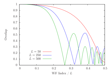
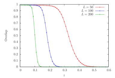
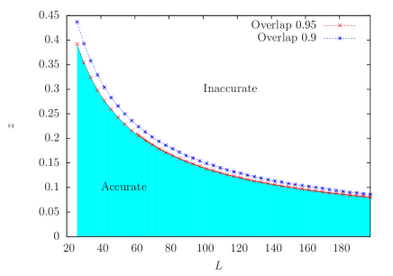
Figure 4: Top left: overlap between continuum approximation and numerical single-particle wavefunctions, in a one-to-one basis, for $z=1$. Top right: overlap between continuum and numerical many-body states, as a function of $z$, for different values of $L$. Bottom: validity region for the continuum approximation, showing the lines of $90\%$ and $95\%$ overlap between the continuum and the exact wavefunctions.

Even if the wavefunctions are not correctly predicted in a one-to-one basis, the complete Slater determinant composing the states can be similar. This possibility is checked in the top-right panel of Fig. 4, where we plot the overlap between the full Slater determinant states (continuum limit and numerical computation) as a function of $z$ for different values of the system size $L$. We can see that below a certain critical $z$, the overlap stays close to one, and then it decreases to zero.

The bottom panel of Fig. 4 shows the region of validity of the continuum approximation in the $(L,z)$ plane, by depicting two lines which mark the level 0.95 and the level 0.9 for the overlap between the numerical GS of the Hamiltonian and the continuum approximation obtained by the deformed uniform wavefunctions.

IV Entanglement Structure

The most relevant fact about the entanglement structure of the GS of Eq. (7) is that the von Neumann entropy scales linearly with the system size –i.e., with a volume law– as soon as $\alpha<1$, with a prefactor that was determined numerically in Ramirez.rainbow.14 as $\approx-\log(\alpha)/6$. Can this prefactor be explained?

IV.1 Entanglement in the continuum approximation

The von Neumann entropy of the left half of a critical system with open boundary conditions and size $L$ is given by

$$S_{CFT}(L)={c\over 6}\log(L)+c^{\prime},$$ (34)

where $c$ is the central charge of the model, and $c^{\prime}$ is an additive constant that includes the boundary entropy plus non-universal contributions Vidal.PRL.03 ; Calabrese.JSTAT.04 . For the free fermionic system under study, $\alpha=1$, we have $c=1$. Taking in combination Eqs. (34) and (28), we can provide a prediction for the entropy of the half-chain in the deformed GS of (7). Indeed, substituting $L$ by $\tilde{L}$, we obtain

$$S_{CSP}(L)={c\over 6}\log\left({e^{hL}-1\over h}\right)+c^{\prime},$$ (35)

which is checked in Fig. 5 (left) for low values of $h$, although its validity ranges far beyond that regime close to the conformal point.

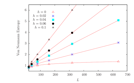
Figure 5: Comparing the half-chain entropy for different $L$ and $h$ with the theoretical prediction, Eq. (35).

Expression (35) can be expanded in the limit when $hL$ is large enough as

$$S_{CSP}(L)\approx{c\over 6}hL,$$ (36)

in agreement with numerical estimation (15) of Ramirez.rainbow.14 ,

$$S_{L}\approx-0.318\;L\;\log(\alpha),$$ (37)

since $h/2=-\log(\alpha)$. Notice also that in the limit $h\to 0^{+}$, one recovers the expression (34).

It is worth to compare Eq. (35) with the entropy of a thermal state at inverse temperature $\beta=1/T$ in a CFT Calabrese.JSTAT.04

$$S_{CFT}(L)\approx\frac{c}{3}\log\left(\frac{\beta}{\pi}\sinh\left(\frac{\pi L}{\beta}\right)\right)\approx\frac{\pi cL}{3\beta},$$ (38)

where we have taken the limit $L\gg\beta$, which leads to an extensive entropy. Comparing Eq. (38) and Eq. (36) we obtain that

$$T=\frac{1}{\beta}=\frac{h}{2\pi},$$ (39)

in agreement with Eq. (32), which was based on the analytic extension of the transformation employed to derive the continuum limit, Eq. (27). In other words, we can assert that the rainbow state is similar to a thermal state with temperature given by $h$.

IV.2 Rényi entropies

Let us focus our attention on Rényi entropies, defined as:

$$S^{(n)}_{A}=\frac{1}{1-n}\log{\rm Tr}_{A}\rho^{n}_{A},$$ (40)

where $A$ is a block with $\ell$ sites and $\rho_{A}$ is the corresponding density matrix. The von Neumann entropy can be obtained as the limit $n\to 1$ of $S^{(n)}_{A}$. The expression of $S^{(n)}_{A}$ for the GS of the free fermion model on an open chain of length $2L$ is given by

$$S_{\ell}^{(n)}\simeq\frac{c}{12}\left(1+\frac{1}{n}\right)\log{\left[\frac{4L}{\pi}\sin{\left(\frac{\pi\ell}{2L}\right)}\right]}+c^{\prime}_{n}+f_{n}\cos{(\pi\ell)}\left[\frac{8L}{\pi}\sin{\left(\frac{\pi\ell}{2L}\right)}\right]^{-K/n},$$ (41)

where $\ell$ is the length of the block $A$ that is located at either boundary of the chain. The first term is the familiar CFT contribution with $c=1$, while the second term contains the fluctuations at Fermi momentum $k_{F}=\pi/2$. $K$ is the Luttinger parameter which in our case is equal to $1$. The constants $f_{n}$ have also been computed analytically in reference Fagotti.JSTAT.11

$$f_{1} = -1$$

$$f_{n} = \frac{2}{1-n}\frac{\Gamma\left(\frac{1}{2}+\frac{1}{2n}\right)}{\Gamma\left(\frac{1}{2}+\frac{1}{2n}\right)}\qquad(n>1).$$ (42)

Let us consider the left-half block. According to (41), the Rényi entropy of order $n$ is given by

$$S_{L}^{(n)}\simeq\frac{1}{12}\left(1+\frac{1}{n}\right)\log{\left(\frac{4L}{\pi}\right)}+c^{\prime}_{n}+f_{n}\cos(\pi L)\left(\frac{8L}{\pi}\right)^{-1/n}.$$ (43)

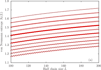
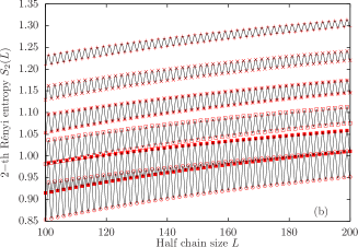
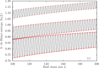
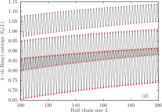
Figure 6: Rényi entanglement entropy at half chain. All panels show $z=\{0,0.4,0.8,\cdots,4\}$ from bottom to top, and fits are made to expression (44). From top to bottom, and left to right, orders $n=1$ (von Neumann), $2$, $3$ and $4$ of the Rényi entropy.

Moving into the rainbow phase, we can give a first estimate of the Rényi entropies using the SDRG prescription. According to it, they are all equal among themselves, and equal to the von Neumann entropy Ramirez.rxx.14 . This approximation becomes exact only in the $\alpha\to 0^{+}$ limit. Otherwise, we should make use of the following exact diagonalization strategy Ramirez.rxx.14 ; Peschel.JPA.03 :

1. Obtain the occupied single-body wavefunctions $\psi^{k}$.

2. Compute the correlation matrix, $C_{ij}=\langle GS|c^{\dagger}_{i}c_{j}|GS\rangle=\sum_{k}\bar{\psi}^{k}_{i}\psi^{k}_{j}$, with $i$ and $j$ both inside the considered block.

3. Diagonalize matrix $C$ and obtain its eigenvalues $\{\nu_{p}\}$.

4. The Rényi entropy is then given by $S^{(n)}_{B}={1\over 1-n}\sum_{p}\log(\nu_{p}^{n}+(1-\nu_{p})^{n})$.

The numerical computations performed as above can be compared to a natural extension of expression (43):

$$S_{L}^{(n)}(z)=\frac{c_{n}(z)}{12}\left(1+\frac{1}{n}\right)\log{\left(\frac{4L}{\pi}\right)}+d_{n}(z)+f_{n}(z)(-1)^{L}\left(\frac{8L}{\pi}\right)^{-1/n}.$$ (44)

This equation is a generalization of the Ansatz made in reference Ramirez.rainbow.14 for the von Neumann entropy of the half-chain $S_{L}^{(1)}(z)$. The comparison is performed in Fig. 6, which shows the Rényi entropies at half chain for different values of $z$ in each panel, fitting the parameters $c_{n}(z)$, $d_{n}(z)$ and $f_{n}(z)$. The Luttinger constant is kept as $K=1$. Oscillations in all cases decrease as $z$ increases, but they always increase with the Rényi order $n$.

The functions $c_{n}(z)$, $d_{n}(z)$ and $f_{n}(z)$, are shown in Fig. 7. Their expression can be derived replacing $L$ by $\tilde{L}$ in Eq. (28), and writing

$$\tilde{L}=\frac{e^{z}-1}{z}L,$$ (45)

which yields

$$c_{n}(z)=1,\qquad d_{n}(z)=c^{\prime}_{n}+\frac{c}{12}\left(1+\frac{1}{n}\right)\log\left(\frac{e^{z}-1}{z}\right),\quad f_{n}(z)=f_{n}\left(\frac{e^{z}-1}{z}\right)^{-1/n},$$ (46)

Fig. 7 shows the fitting coefficients for different orders of the Rényi entropy, Eq. (44), for systems of size $10^{2}\leq L\leq 10^{3}$ and for a range of values $0\leq z\leq 20$. Panel (a) shows the small variation ($<4\cdot 10^{-2}$) for $c_{n}(z)$ in all range of $z$. Panels (b-c) show $d_{n}(z)$ and $f_{n}(z)$, solid lines are given by Eq. (46). Notice the perfect agreement between these expressions and the numerical results.

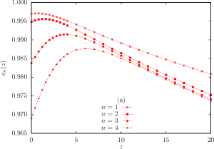
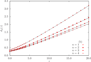
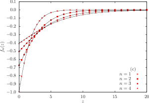
Figure 7: Fitting parameters in Eq. (44) as a function of $z$: (a) $c_{n}(z)$, where the lines are for visual guide only; (b) $d_{n}(z)$, where the continuous line is given in Eq. (46) (c) $f_{n}(z)$, where the continuous line is given in Eq. (46).

IV.3 Entanglement spectrum and thermofield states

The entanglement spectrum (EE) of this model was already considered in Ramirez.rainbow.14 . It is given by the eigenvalues of the entanglement Hamiltonian $H_{E}$, that is defined in terms of the reduced density matrix $\rho_{A}$ as $\rho_{A}=e^{-H_{E}}$. Let us summarize the results obtained in Ramirez.rainbow.14 and provide an interpretation from the perspective obtained in the previous sections. The entanglement Hamiltonian $H_{E}$ has the form

$$H_{E}=\sum_{p}\epsilon_{p}b^{\dagger}_{p}\,b_{p}+f_{0},$$ (47)

where $b_{p},b^{\dagger}_{p}$ are destruction and annihilation fermion operators, and $\epsilon_{p}$ are related to the eigenvalues of the correlation matrix in the block $A$ (for details see Ramirez.rainbow.14 ). For large values of $L$, the energies $\epsilon_{p}$ are given approximately by

$$\epsilon_{p}\simeq\Delta_{L}\,p,\quad p=\left\{\begin{array}[]{cc}\pm\frac{1}{2},\pm\frac{3}{2},\dots,\pm\frac{L-1}{2}&L:{\rm even},\\ 0,\pm 1,\pm 2,\dots,\pm\frac{L-1}{2}&L:{\rm odd}.\\ \end{array}.\right.$$ (48)

The level spacing $\Delta_{L}$ in turn was found in Ramirez.rainbow.14 to be related to the half-chain entropy $S_{L}$ as

$$S_{L}\approx\frac{\pi^{2}}{3\Delta_{L}},$$ (49)

which, using Eq. (28) and (32), implies

$$\Delta_{L}\approx\frac{2\pi^{2}}{hL}=\frac{\pi\beta}{L}.$$ (50)

Hence, the density matrix can be expressed as

$$\rho_{A}\approx e^{-\beta H_{CFT}},\qquad H_{CFT}=\frac{\pi}{L}\sum_{p}p\,b^{\dagger}_{p}\,b_{p},$$ (51)

where $H_{CFT}$ is the CFT Hamiltonian of half of the chain. Thus, the single-body entanglement energies should fulfill, for different values of $L$ and $z$, the following law:

$$\epsilon_{p}\simeq\beta\,\epsilon_{p}^{CFT}=\left({2\pi\over h}\right)\,\left({\pi\over L}\,p\right)={2\pi^{2}\over z}\,p,$$ (52)

which we can see confirmed in the results of Fig. 8.

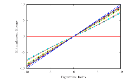
Figure 8: Entanglement single-body energies $\epsilon_{p}$ for different values of $L$ (60 to 160) and $z$ ($5$ to $L$ in each case), multiplied by $z/(2\pi^{2})$. As predicted, they collapse to the diagonal line, following Eq. (52), $\epsilon_{p}\simeq 2\pi p/z$.

We then arrive at the conclusion that the CSP state can be written as

$$|\psi_{CSP}\rangle=\sum_{n}e^{-\beta E_{n}/2}|n\rangle_{L}\,|n\rangle_{R},$$ (53)

where $|n\rangle_{R}$ and $|n\rangle_{L}$ are orthonormal basis for the right and left pieces of the chain whose Hamiltonians are isomorphic to $H_{CFT}$ in Eq. (51). A pure state of the form (53) is called a thermofield state and has been employed in connection with black holes and the EPR=ER conjecture Hartman.JHEP.13 ; Maldacena.FPhys.13 . In these studies, $T=1/\beta$ is the temperature of the black hole that can be expressed as $a/(2\pi)$ where $a$ is the acceleration of a Rindler observer. Looking at Eq. (39), we see that the constant $h$ plays that role in our model.

Numerical evidence for other cases where $\rho\sim e^{-H_{CFT}}$ was explored before using different scalings Lauchli.13 .

V Two-dimensional extension

A natural question is: can the 1D results be extended to 2D? In other terms, can we find a local 2D Hamiltonian whose GS violates maximally the area law? We shall next show that this is indeed possible in a rather simple way.

Let us consider a $2L\times 2L$ square lattice whose sites are labeled by $X=(x,y)$ with $x,y\in\{\pm 1/2,\pm 3/2,\cdots,\pm(L/2-1/2)\}$. We define a hopping Hamiltonian of the form:

$$H=-\sum_{\langle X,X^{\prime}\rangle}J_{X,X^{\prime}}c^{\dagger}_{X}c_{X^{\prime}}+\mathrm{h.c.}$$ (54)

with $J_{X,X^{\prime}}=F\left((X+X^{\prime})/2\right)$ is only determined by the center of the segment joining points $X$ and $X^{\prime}$. In our case, we choose $F(x,y)=\alpha^{|x|}$, to resemble the 1D analogue. Fig. 9 represents graphically a small region near the center.

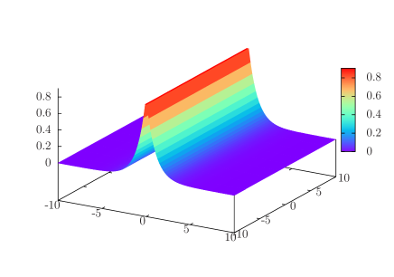
Figure 9: Left: a small region of the $2L\times 2L$ square lattice used to generate the 2D rainbow state. The nodes represent the sites, and the number attached to the link is the associated hopping amplitude, given by $\alpha^{|x|}$, with $x$ the horizontal coordinate of the middle point. Right: 3D view of the structure of the hopping distribution.

Fig. 10 shows the entropy per unit length of a block composed of the left half of the system $s_{L}(\alpha)=S_{L}(\alpha)/L$ for different values of the coupling parameter $\alpha$. The solid lines represent fits to an expression of the form

$$s_{L}(\alpha)\simeq A(\alpha)L+B(\alpha)\log(L)+C(\alpha),$$ (55)

where a non-zero linear term denotes a volumetric behavior of the entanglement entropy, and the logarithmic term is added in order to predict the correct behavior for $\alpha\to 1^{-}$ Klich.06 . The fits can be seen in table 1. Notice the low values of $\chi^{2}$ for $\alpha<1$ and the increase of the volume coefficient with $\alpha$.

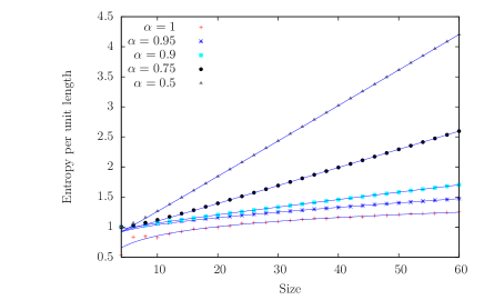
Figure 10: Entanglement entropy of the left half of the system, per unit length of the boundary, for different values of $\alpha$ for a 2D concentric singlet phase.

Table 1: Fitting parameters for the 2D entropy function in equation (55)

$\alpha$	$A(\alpha)$	$B(\alpha)$	$C(\alpha)$	$\chi^{2}$
1	0	0.234	0.29	$3\cdot 10^{-5}$
0.95	0.0053	0.0940	0.77	$10^{-9}$
0.9	0.0116	0.0330	0.87	$10^{-9}$
0.75	0.0307	-0.0225	0.85	$10^{-9}$
0.5	0.0594	-0.015	0.70	$10^{-9}$

VI Conclusions and further work

In this work we have extended the previous studies of the concentric singlet state, or rainbow state Vitagliano.NJP.10 ; Ramirez.rainbow.14 , which is a deformation of a 1D system which exhibits a volume law for the entanglement entropy. We focus on a free fermion realization in order to benefit from the exact solubility. The extension presented in this article is based on the application of field-theory methods. We show that, in the vicinity of the conformal model, the ground state can be described by a map that is the union of the conformal maps associated to each half of the chain. The corresponding conformal transformations further suggest the definition of a temperature that is proportional to the parameter controlling the decay of the hopping parameters. We show how this deformation accounts for the change in the dispersion relation, the single-particle wavefunctions in the vicinity of the Fermi point, and the half-chain von Neumann and Rényi entropies. The appearance of a volume law entropy is linked to the existence of an effective temperature for the GS that is finally identified with a thermofield state. This striking result points towards an unexpected connection with the theory of black holes and the emergence of space-time from entanglement.

Finally, we show how to extend the rainbow Hamiltonian to several dimensions in a natural way, and check that the entanglement entropy of the two-dimensional analogue grows as the area of the block.

Appendix A Qubistic picture

Qubism Laguna.NJP.12 is a pictographic representation for quantum many-body states with the peculiarity that it allows for the visualization of entanglement. In summary, an $N$ qubit wavefunction is shown on the $[0,1]^{2}$ square divided into $2^{N/2}\times 2^{N/2}$ cells. Each of the $2^{N}$ wavefunction component are depicted into one of the cells, following a recursive pattern, in which the $i$-th qubit is associated with the $i$-th length scale, in decreasing order.

Fig. 11 represents the qubistic plots of the rainbow ground state for two different sizes, $2L=10$ and $2L=12$, and three values of $\alpha=0.01$, $0.3$ and $1$. Therefore, the rightmost panels correspond to the ground state of the free fermion model, and the leftmost panels represent the rainbow states. Notice that the representation is formed only by a finite and small set of points.

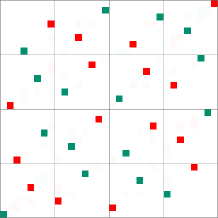
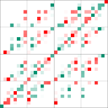
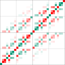
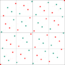
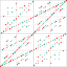
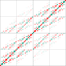
Figure 11: Qubistic picture of the rainbow state for different sizes of the system $2L=10$ and $2L=12$ (upper and lower rows) and three values of $\alpha=0.01$, $0.3$ and $1$ (left to right columns). Color intensity denotes the wavefunction amplitude and hue denotes phase: red is positive and green negative.

Entanglement between the first pair of qubits and the rest can be visualized in the following way Laguna.NJP.12 . Break the full square into $2\times 2$ square of half-size. Count the number of different (strictly, linearly independent) images among the small squares. That number is an upper bound for the Schmidt rank, which is a measure of entanglement. The same procedure can continue, for the block composed of the first four qubits, if we decompose the original square into a $4\times 4$ grid. In our case, notice that the dots in each of the small squares form a similar but different pattern. In fact, the number of different (independent) images coincides with the number of squares, $4$ for the first two qubits, $16$ for the first four, etc. This shows that the Schmidt rank grows as $2^{\ell}$, i.e., entanglement is maximal.

References

- (1) L. Amico et. al., Rev. Mod. Phys., 80, 517–576 (2008).
- (2) M. Sredniki, Phys. Rev. Lett. 71, 666 (1993).
- (3) J. Eisert, M. Cramer, M. B. Plenio, Rev. Mod. Phys. 82 277 (2010).
- (4) M. B. Hastings, J. Stat. Mech. P08024 (2007).
- (5) C. Holzhey, F. Larsen and F. Wilczek, Nucl. Phys. B 424, 443 (1994).
- (6) G. Vidal, J. I. Latorre, E. Rico and A. Kitaev, Phys. Rev. Lett. 90 227902 (2003)
- (7) P. Calabrese and J. Cardy, J. Stat. Mech. P06002 (2004).
- (8) L. Huijse and B. Swingle, Phys. Rev. B 87, 035108 (2013).
- (9) G. Gori, S. Paganelli, A. Sharma, P. Sodano and A. Trombettoni, ArXiv:1405.3616.
- (10) G. Vitagliano, A. Riera, and J. I. Latorre, New J. Phys. 12, 113049 (2010).
- (11) G. Ramírez, J. Rodríguez-Laguna and G. Sierra, J. Stat. Mech., P10004 (2014).
- (12) M. Vekić and S. R. White, Phys. Rev. Lett. 71, 4283 (1993).
- (13) K. Okunishi and T. Nishino, Phys. Rev. B 82, 144409 (2010).
- (14) H. Ueda and T. Nishino, Journal of the Physical Society of Japan 78, 014001 (2009).
- (15) H. Ueda, H. Nakano, K. Kusakabe, and T. Nishino, Progress of Theoretical Physics 124, 389 (2010).
- (16) J. Rodríguez-Laguna, P. Migdał, M. Ibáñez-Berganza, M. Lewenstein and G. Sierra, New J. Phys 14, 053028 (2012).
- (17) C. Dasgupta and S-K Ma, Phys. Rev. B 22, 1305 (1980).
- (18) G. Ramírez, J. Rodríguez-Laguna and G. Sierra, J. Stat. Mech., P07003 (2014).
- (19) In order to obtain further insight into the reason for this transformation, consider a one-dimensional chain of sites, numbered to , where two singlet bonds are established, between sites and , and between sites and . When transformed, via the Jordan-Wigner transformation, into a fermionic state, it becomes .
- (20) Notice a change of notation and normalization as compared to Ref. Ramirez.rainbow.14 .
- (21) K. G. Wilson, Rev. Mod. Phys. 47, 773 (1975).
- (22) Due to the different normalization conventions, the parameter used in Ramirez.rainbow.14 is equal to used in this paper.
- (23) M. Fagotti and P. Calabrese, J. Stat. Mech. P01017 (2011).
- (24) I. Peschel, J. Phys. A.: Math. Gen. 36, L205 (2003).
- (25) T. Hartman and J. Maldacena, JHEP 2013:14.
- (26) J. Maldacena and L. Susskind, Fortschr. Phys. 61, 781 (2013).
- (27) A. M. Läuchli, ArXiv:1303.0741.
- (28) D. Gioev and I. Klich, Phys. Rev. Lett. 96, 100503 (2006).