APPLICATION OF GAS DYNAMICAL FRICTION FOR PLANETESIMALS:
I. EVOLUTION OF SINGLE PLANETESIMALS

Abstract

The growth of small planetesimals into large planetary embryos occurs much before the dispersal of the gas from the protoplanetary disk. The planetesimal - gaseous-disk interactions give rise to migration and orbital evolution of the planetesimals/planets. Small planetesimals are dominated by aerodynamic gas drag. Large protoplanets, $m\sim 0.1M_{\oplus}$, are dominated by type I migration differential torque. There is an additional mass range, $m\sim 10^{21}-10^{25}g$ of intermediate mass planetesimals (IMPs), where gravitational interactions with the disk dominate over aerodynamic gas drag, but for which such interactions were typically neglected. Here we model these interactions using the gas dynamical friction (GDF) approach, previously used to study the disk-planet interactions at the planetary mass range. We find the critical size where GDF dominates over gas drag, and then study the implications of GDF on single IMPs. We find that planetesimals with small inclinations rapidly become co-planar. Eccentric orbits circularize within a few Myrs, provided the the planetesimal mass is large, $m\gtrsim 10^{23}g$ and that the initial eccentricity is low, $e\lesssim 0.1$. Planetesimals of higher masses, $m\sim 10^{24}-10^{25}g$ inspiral on a time-scale of a few Myrs, leading to an embryonic migration to the inner disk. This can lead to an over-abundance of rocky material (in the form of IMPs) in the inner protoplanetary disk ($<1$AU) and induce rapid planetary growth. This can explain the origin of super-Earth planets. In addition, GDF damps the velocities of IMPs, thereby cooling the planetesimal disk and affecting its collisional evolution through quenching the effects of viscous stirring by the large bodies.

1. INTRODUCTION

Planets form in protoplanetary disks around young stars. Once km sized planetesimals have been formed, their evolution is determined by three basic dynamical processes: Viscous stirring, dynamical friction and coagulation or disruption through collisions (see Goldreich et al., 2004 and references therein for details). These dynamical processes do not include the effects from planetesimal-gas interaction in the disk, which can be important during the early stages of planet formation when gas is abundant (the first few Myr, with possible suggestions for longer time-scales, Pfalzner et al., 2014).

During the evolutionary phases of planet formation, small dust grains successively grow to large planetary embryos. For small size planetesimals, aerodynamic gas drag is the dominant effect of the gas. It maintains low relative velocities and keeps the orbits circular and co-planar. Hence, the planetesimal disk is expected to be thin (Ohtsuki et al., 2002). It may also assist in the coagulation and merger of small bodies (Ormel & Klahr, 2010; Perets & Murray-Clay, 2011). Large planetary embryos ($m\geq 0.1M_{\oplus})$ can migrate due to the interaction with the gaseous disk (see e.g. Papaloizou & Terquem, 2006 for a review and references therein.)

Gas-planetesimal interactions are therefore important both for low mass planetesimals and large earth-sized or larger embryos. However, there exists an intermediate planetesimal mass (IMP) range, of the order of $m\sim 10^{21}-10^{25}g$ in which gas-planetesimal interactions are typically neglected, since such planetesimals are large enough to be fully decoupled from the gas, and aerodynamic gas drag is too weak to affect their gravitational dynamics, while they are not sufficiently massive to exert significant torque on the ambient gas and change its global properties (Hourigan & Ward, 1984; Tanaka & Ida, 1999). Nevertheless, in this mass range, gravitational interactions with the disk are not negligible, and the disk-planetesimal interactions can be modeled through gas dynamical friction (GDF), which dominates over aerodynamic gas drag. Here we focus on the effects of GDF on IMP and consider its role in their dynamical evolution.

Ostriker (1999) showed that dynamical friction in gaseous medium exerts a force even at low subsonic velocities. GDF is important for various astrophysical systems: migration of globular clusters in galactic gaseous haloes, in-spiral of binary stars in the companion’s envelope and merger and in-spiral of binary black holes (e.g. Stahler 2010; Escala et al. 2004b, a; Baruteau et al. 2011). Moreover, it was estimated that aerodynamic drag is comparable to GDF for bodies as large as a few hundred km in diameter. Direct applications of GDF on planetary systems with sufficiently large eccentricities and inclinations have been recently studied (Teyssandier et al., 2013; Cantó et al., 2013; Rein, 2012; Muto et al., 2011), however they deal with masses of fully formed planets, above the IMP range. Various generalizations of GDF are found in the literature; e.g. numerical modeling, circular orbits in the non-linear regime and others (Sánchez-Salcedo & Brandenburg 2001; Kim & Kim 2007; Kim et al. 2008; Kim & Kim 2009; Kim 2010), and more recently Muto et al. (2011) obtained formulae for GDF in 2D slab geometry, directly applicable to protoplanetary disks.

Motivated by recent developments both in GDF theory and its application to planetary systems, we explore the implications of GDF on single IMP. The implications on binary planetesimals will be discussed in a subsequent paper (Grishin & Perets, in prep.). To do so we review and compare the effects of aerodynamic gas drag (Section 2.1) and GDF (Section 2.2) and derive the typical size of planetesimals for which GDF dominates over gas drag (Section 2.3). We then calculate the time-scales for variation of orbital elements using analytical arguments, and study GDF effects numerically (Section 3). Finally, we discuss (Section 4) the implications of such processes for the evolution planetesimals.

2. GAS PLANETESIMAL INTERACTION

The standard models of evolution of planetesimal disks account for various dynamical processes, including both physical processes due to planetesimal interactions such as viscous stirring, dynamical friction and physical collisions followed by coagulation, as well as gas-planetesimal interactions through aerodynamic gas-drag on small planetesimals, and planetary migration through disk torques acting on large planetary embryos and planets.

Although gas-planetesimal interaction has been studied in the context of small planetesimals, massive planetesimals have been largely ignored as they are decoupled from the gas, and their size and velocity dispersion is dominated by gravitational interactions. In the following, we revisit this argument by carefully examining processes caused due to the presence of gas and discuss their possible implications. We first review the basic properties of aerodynamic gas drag and GDF respectively, and then compare both forces and find the lower limit of the planetesimal size for which GDF becomes dominant compared with aerodynamic gas drag. The lower limit is found to be roughly in the order of a few hundred km, compatible with Ostriker (1999)’s estimation, and depends on the position in the disk and its gas density.

2.1. Aerodynamic gas drag

The general drag force imposed on a planetesimal of radius $R$ and relative velocity $v_{rel}$ moving through a gaseous medium of density $\rho_{g}$ and speed of sound $c_{s}$ depends on $R/\lambda$, where $\lambda=1/n\Gamma$, is the mean free path of the gas, $n$ is the number density of the gas, and $\Gamma$ is the cross section of gas-gas collisions.

When $R\lesssim\lambda$, Epstein regime applies where individual scattering is considered. The drag force is

$$\boldsymbol{F}_{D}=-\frac{4}{3}\pi R^{2}\rho_{g}\bar{v}_{th}\boldsymbol{v}_{rel}$$ (1)

Where $\bar{v}_{th}=(8/\pi)^{1/2}c_{s}$ is the mean thermal velocity (for Maxwellian distribution).

For $R\gtrsim\lambda$, the gas must be modeled as a fluid. Here, the drag force depends also on the Reynolds number $\mathcal{R}e=2Rv_{rel}/\nu_{m}$, where $\nu_{m}=(1/2)\bar{v}_{th}\lambda$ is the molecular viscosity of the gas. For high Reynolds numbers ($\mathcal{R}e\gtrsim 800$) the gas exerts a ram pressure force, while for lower Reynolds numbers Stokes drag is more applicable. The drag force is

$$\boldsymbol{F}_{D}=-\frac{1}{2}C_{D}\pi\rho_{g}v_{rel}^{2}\hat{\boldsymbol{v}}_{rel}$$ (2)

where $C_{D}$ is the drag coefficient and $\hat{\boldsymbol{v}}_{rel}$ is the unit vector in the direction of relative velocity. Generally $C_{D}$ depends on the geometry of the object, but for spherical objects it depends only on Reynolds number, i.e. $C_{D}=C_{D}(\mathcal{R}e)$. An empirical formula can be used for $C_{D}(\mathcal{R}e)$, fitted for the range $\log_{10}\mathcal{R}e\in[-3,5]$ by Brown & Lawyer (2003).

$$C_{D}(\mathcal{R}e)=\frac{24}{\mathcal{R}e}(1+0.27\mathcal{R}e)^{0.43}+0.47[1-\exp(-0.04\mathcal{R}e^{0.38})]$$ (3)

In the large Reynolds number limit $C_{D}$ is constant, while in the low Reynolds number limit $(\mathcal{R}e<1)$, $C_{D}\sim\mathcal{R}e^{-1}$. From consistency of Eq. (1) and Eq. (2), the transition between Epstein and Stokes drag regimes is $R\approx(9/4)\lambda$, and $C_{D}=24/\mathcal{R}e$ for $\mathcal{R}e<1$.

2.2. Gas dynamical friction

Consider a perturber with mass $m_{p}$ moving on a straight line with constant velocity $\boldsymbol{v}_{rel}$ in a uniform gaseous medium with density $\rho_{g}$ and characteristic sound speed $c_{s}$. The perturber generates a wake, which in turn affects the perturber. Using linear perturbation theory, Ostriker (1999) calculated the gravitational drag force felt by the perturber. The gas dynamical friction (GDF) force is given by

$$\boldsymbol{F}_{GDF}=-\frac{4\pi G^{2}m_{p}^{2}\rho_{g}}{v_{rel}^{3}}\boldsymbol{v}_{rel}\mathcal{I}(\mathcal{M})$$ (4)

where $\mathcal{M}\equiv v_{rel}/c_{s}$ is the Mach number, and $\mathcal{I}(\mathcal{M})$ is a dimensionless factor given by

$$\mathcal{I}(\mathcal{M})=\left\{\begin{array}[]{cc}\frac{1}{2}\ln\left(\frac{1+\mathcal{M}}{1-\mathcal{M}}\right)-\mathcal{M}&\mathcal{M}<1\\ \frac{1}{2}\ln\left(1-\frac{1}{\mathcal{M}^{2}}\right)+\ln\left(\frac{v_{rel}t}{R_{min}}\right)&\begin{array}[]{cc}\mathcal{M}>1\\ v_{rel}t>R_{min}\end{array}\end{array}\right.$$ (5)

The force is non-vanishing in the subsonic regime, while in the supersonic regime, a minimal radius $R_{min}$ is introduced to avoid divergence of the gravitational potential (usually taken to be the physical size of the perturber, or the accretion radius $Gm_{p}/v_{rel}^{2}$). The exact value of $R_{min}$ is not well determined; but it can be fitted through comparison of Eq. (5) with hydrodynamical simulations, to find a best fitting value for $R_{min}$ (Sánchez-Salcedo & Brandenburg, 1999). It is important to stress that Ostriker’s original calculation was done using a point mass perturber; GDF is a gravitational volume force, essentially different from the aerodynamic drag, which is a surface force, dependent on the geometry of the perturber.

For small Mach numbers $\mathcal{M}\ll 1$,

$$\mathcal{I}(\mathcal{M})=\mathcal{M}^{3}/3+O(\mathcal{M}^{5})$$ (6)

We note that the results of Kim & Kim (2007) are qualitatively similar to Ostriker’s straight line trajectory (see fig. (8) of Kim & Kim, 2007). Comparison to Muto et al. (2011)’s formulae for slab geometry and validity of both models is discussed in Section 4.1.

2.3. Comparison between gas dynamical friction and aerodynamic gas drag

Aerodynamic drag is more dominant for small size planetesimals and scales as $\sim R^{2}$. GDF is negligible for small sizes, and scales as $\sim R^{6}$, since $m\sim\rho_{m}R^{3},$ where $\rho_{m}$ is the material density.

It is therefore clear that there exists a unique value $R_{\star}(G,\rho_{m},v_{rel},\mathcal{R}e,\mathcal{M})$ for which the aerodynamic drag and GDF forces are equal. Moreover, $R_{\star}$ is not dependent on $\rho_{g}$. The only independent dimensional parameters are $G,\rho_{m}$ and $v_{rel}$. Dimensional analysis shows that $R_{\star}$ scales as $R_{\star}\propto v_{rel}(G\rho_{m})^{-1/2}$, where the proportion constant depends on the dimensionless numbers $\mathcal{R}e,$ and $\mathcal{M}$. Comparing equations (2) and (4) then yields the critical size

$$R_{\star} = 0.29\left[\frac{C_{D}(Re)}{\mathcal{I}(\mathcal{M})}\right]^{1/4}\frac{v_{rel}}{\sqrt{G\rho_{m}}}$$ (7)

The radial drift of the gas is slightly sub-Keplerian due to pressure gradients. For circular orbits, the radial drift velocity of the gas is $\boldsymbol{v}_{gas}=\boldsymbol{v}_{K}\sqrt{1-\eta},$ where

$$\eta=-\frac{\partial P/\partial\ln a}{2\rho_{g}v_{K}^{2}}$$ (8)

(Chiang & Youdin, 2010). For flat razor-thin disk, $\Sigma\propto a^{-1}$ , $P\propto a^{-3}$ we get $\eta=3H_{0}^{2}$, where $H_{0}=h/a\sim c_{s}/v_{K}$ is the aspect ratio of the disk (Armitage, 2013).

Consider a planetesimal travelling in a circular orbit in a gaseous disk. The relative velocity of the headwind is $\boldsymbol{v}_{rel}=\boldsymbol{v}_{K}-\boldsymbol{v}_{gas}\equiv K\boldsymbol{v}_{K}$. It is convenient to define $\varepsilon=1-\sqrt{1-\eta}\approx\eta/2+\mathcal{O}(H_{0}^{4})$. Thus, using (8), $K=\varepsilon$. For typical ranges of $H_{0}\in[0.01,0.05]$, the range of $\varepsilon$ is $\approx[10^{-4},4\cdot 10^{-3}]$.

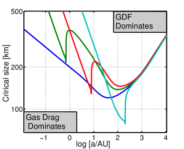
Figure 1.— Numerical solution for equation (7) for various eccentricities. Top: Critical size of planetesimal as a function semi-major axis. Each curve corresponds to different orbital eccentricity $e$, and indicates the critical size $R_{\star}(a)$ where both forces are equal. Aerodynamic drag dominates for smaller radii, while GDF dominates for larger radii. Note log-log scale. Bottom: Estimated Mach number as a function of semi-major axis for the same orbits. Note the logarithmic scale.

For a concrete example, we consider a disk with similar parameters as used by Perets & Murray-Clay (2011). The disk scaling is adapted from Chiang & Goldreich (1997)’s simple flared disk model. Let us consider a specific power law scaling of disk parameters, with respect to distance, $a$, to the central star. Disk temperature is $T=120(a/AU)^{-3/7}K$. Molecular weight is $\mu=2.3m_{H}$, where $m_{H}=1.66\cdot 10^{-24}g$ is the hydrogen atom mass. This leads to $c_{s}=(k_{B}T/\mu)^{1/2}=6.63\cdot 10^{4}(a/AU)^{-3/14}cm\cdot s^{-1}$. The disk aspect ratio is $H_{0}=h(a)/a=0.022(a/AU)^{2/7}$, where $h(a)$ is the disk scale height.

For full evaluation of the relative velocities we will relax our assumption of circular orbits and let the eccentricity, $e$, be a free parameter. We show in appendix A that the ratio of the relative and the Keplerian velocity $K=v_{rel}/{v_{K}}$ alters to $K\approx\sqrt{\varepsilon^{2}+e^{2}}+\mathcal{O}(e^{4})$. A more complete treatment of the relative velocity between an eccentric orbit and a planet is given in Muto et al. (2011). The Reynolds number is $Re=2Rv_{rel}/\nu_{m}$, where $R$ is the planetesimal size, $\nu_{m}\sim c_{s}\lambda$ is the molecular viscosity, and $\lambda$ is the mean free path. Note that although Eq. (7) appears simple, $C_{D}$ depends on $\mathcal{R}e$ via Eq. (3), which in turn depends on $R_{\star}$.

The top panel of Fig. 1 shows the numerical solution of Eq. (7). We see that for low eccentricities, planetesimals with $R\gtrsim 500km$ are dominated by GDF for most regions of the disk. We see that the derivative of the solution $R_{\star}(a,e)$ is discontinuous where the Mach number $\mathcal{M\approx}1$. It happens approximately where $e=H_{0},$ the disk aspect ratio. The origin of the discontinuity is the simplified discontinuous behavior of $\mathcal{I}(\mathcal{M})$ near $\mathcal{M\approx}1$ given in Eq. (5).

The bottom panel of Fig. 1 shows the dependence of the orbit averaged Mach number on $a$. For $H_{0}\ll e$, $v_{rel}=ev_{K}$ and $\mathcal{M}=v_{rel}/c_{s}\propto a^{-2/7}$, i.e. as long as eccentricity is high, the Mach number is a decreasing function of $a$. For $H_{0}\gg e$ , $v_{rel}=\varepsilon v_{K}\approx H_{0}^{2}v_{K}$ and $\mathcal{M}\propto a^{2/7}$ so the Mach number is an increasing function of $a$. The transition occurs when $H_{0}$ is a few times the orbital eccentricity.

In the next sections we will investigate the effects of GDF on single IMPs.

3. GDF EFFECTS ON THE EVOLUTION OF SINGLE PLANETESIMALS

Current studies of gas planetesimal interactions have typically been restricted to the effects of aerodynamic gas drag forces (Youdin, 2010; Goldreich et al., 2004). Here, we implement the effects of GDF for IMPs.

3.1. Formulation of the problem

Consider a planetesimal of mass $m_{p}$ traveling with relative velocity $v_{rel}$ with instantaneous orbital parameters $(a,e,I)$, where $a$ is the semi-major axis, $e$ is the eccentricity and $I$ is the inclination angle.

First, we compute the migration time-scale due to GDF of a circular orbit, and then compare it to N-body simulations with external drag force. For now, we set the inclination to zero, thus the problem has two dimensions. Later on we consider inclined orbits and relax this assumption.

Let us consider a typical gaseous disk with $M_{gas}/M_{\star}\sim H_{0}\sim 0.01$ ($M_{gas}/M_{\star}\sim 0.1$ for most massive disks). Above this limit self gravity is non-negligible and the disk becomes unstable (e.g. Armitage, 2013, and references therein). A typical intermediate mass planetesimal has a diameter of $200-5000$ km, and corresponding mass of $10^{21}-10^{25}g$, where the higher end can already be considered to be a planetary embryo.

We use Ostriker (1999)’s linear theory. Deviations from linear theory and other models are discussed later on.

The problem of accretion of gas by a spherical body was first studied by Bondi, H. (1952). The effective radius of accretion is Bondi radius $r_{B}=2Gm/c_{s}^{2}$. In our case, $r_{B}/r=8\pi G\rho_{m}r^{2}/3c_{s}^{2}=1.25(r/1000km)^{2}.$ Thus for masses lower than $10^{25}g$, accretion is negligible. For a planetary embryo, we estimate the accretion rate by taking $50\%$ accretion efficiency with $\dot{m}\sim 0.5\pi r^{2}\rho_{g}c_{s}\sim 10^{12}g\cdot s^{-1}$. It will take $\tau_{acc}\sim m/\dot{m}\sim 1Myr$ for a planetesimal to accrete its own mass. For simplicity we neglect accretion in our simulations. We’ll briefly discuss the implications of accretion in the summary.

3.2. Timescales for the variation of the orbital elements

Consider a distorting force $\mathbf{F}=F_{r}\hat{\boldsymbol{r}}+F_{\varphi}\hat{\boldsymbol{\varphi}}$. The variation of orbital elements can be calculated analytically. The change in the semi-major axis is (Murray & Dermott, 1999)

$$m_{p}\frac{da}{dt}=2\frac{a^{3/2}}{\sqrt{GM_{\star}(1-e^{2})}}[F_{r}e\sin f+F_{\varphi}(1+e\cos f)]$$ (9)

and

$$m_{p}\frac{de}{dt}=\sqrt{\frac{a(1-e^{2})}{GM_{\star}}}[F_{r}\sin f+F_{\varphi}(\cos f+\cos E)]$$ (10)

where a is the semi-major axis $e$ is the orbital eccentricity and $f$ and $E$ are the true and eccentric anomalies respectively. The relationship between the true and eccentric anomalies is $\tan(f/2)=\sqrt{(1+e)/(1-e)}\tan(E/2)$. For small eccentricies, both anomalies coincide.

The GDF force depends on the relative velocity, hence a crucial step in calculating the interaction between gas and planetesimals is evaluating the relative velocities. The general case is hard to estimate analytically and requires averaging the relative velocity on orbital period (see also Muto et al., 2011), but for small eccentricites (i.e. using equations 4 and 6 the components of the force are $F_{r}=F_{0}v_{rel,r}$ and $F_{\varphi}=F_{0}v_{rel,\varphi}$, where $F_{0}=4\pi G^{2}m_{p}^{2}\rho_{g}/3c_{s}^{3}$ and $v_{rel,r}$ and $v_{rel,\varphi}$ are given by eq’s (A1) and (A2). Neglecting the $(1-e^{2})^{1/2}$ term in the denominator and assuming $\eta\ll 1$, the relative velicities are $v_{rel,r}/v_{K}\approx e\sin f$ and $v_{rel,\varphi}/v_{K}\approx-\eta/2-e\cos f$, which leads to a simplied formulae for Eqs. (9) and (10)

$$\frac{\dot{a}}{a}=2\frac{F_{0}}{m_{p}}\left[-e^{2}\cos(2f)-\frac{\eta}{2}+\left(1-\frac{\eta}{2}\right)e\cos f\right]$$ (11)

and

$$\frac{\dot{e}}{e}=\frac{F_{0}}{em_{p}}\left[-e(\cos(2f)+\cos^{2}f)+\eta\cos f\right]$$ (12)

averaging over one orbit leads us to $\langle\dot{a}/a\rangle=-\eta F_{0}/m_{p}$ and $\langle\dot{e}/e\rangle=-F_{0}/2m_{p}$, where $2\pi\langle A\rangle\equiv\intop_{0}^{2\pi}Adf$ . The typical time-scale for in-spiral is then

$$\tau_{a} =|\langle\frac{a}{\dot{a}}\rangle| =\frac{3}{4\pi\eta}\frac{c_{s}^{3}}{G^{2}\rho_{g}m_{p}}$$ (13)

$$\approx 5.7\cdot 10^{6}\left(\frac{\rho_{g}}{\rho_{0}}\right)^{-1}\left(\frac{m_{p}}{2\cdot 10^{25}g}\right)^{-1}yr$$

Where $\rho_{0}=3\cdot 10^{-9}g\cdot cm^{-3}$. For $m=2\cdot 10^{25}g$ , $\tau_{a}\sim 5.7Myr$, which is comparable with the disk lifetime. Smaller masses are less affected by GDF over the disk lifetime (see also Section 3.4 ). Note that $\tau_{a}$ is inversely proportional to $\rho_{g}.$ At larger separations, $\rho_{g}$ decreases and GDF is less effective. At lower separations GDF stronger, and the rate of in-spiral increases. Thus, $\tau_{a}$ is an upper limit.

For small eccentricity, the eccentricity damping timescale is much faster than the migration timescale (i.e. $\tau_{e}/\tau_{a}=2\eta=6H_{0}^{2}$ ). In addition, the eccentricity decays exponentially, i.e. $\dot{e}\propto e$. The latter is consistent with the analysis of eccentrcity waves raised by a planet studied by Tanaka & Ward, 2004. They find that the decay is exponential and that $\tau_{e}\approx H_{0}^{2}\tau_{a}$ .For larger eccentricities, i.e. $e\gtrsim H_{0}$, the calculation is more complex. Papaloizou & Larwood (2000) find $\dot{e}\propto e^{-2}$ and

$$\tau_{e}/\tau_{a}\approx e^{2}$$ (14)

Both the exponential and the power law decay are confirmed in numerical simulations of type I migration (Cresswell et al., 2007). The connection between type I migration and GDF is discussed in section 4.2

Generally, we expect that the eccentricity to be damped faster than semi-major axis.

The inclination decays rapidly compared with the other orbital elements. Orbital inclination changes due to the $\hat{\boldsymbol{z}}$ component of GDF. For an inclined orbit with inclination angle $I$, the normal force is proportional to $F_{z}\propto v_{z}\sim Iv_{K}$. For a circular orbit, it is much larger than $F_{\varphi}$, since the ambient gas does not possess any significant $\hat{z}$ component for gas velocity. The inclination decay time is then $mdI/dt=\sqrt{a/GM_{\star}}F_{z}\cos(\omega+f)$. Most of the force is applied during the planetesimal passage through the bulk of the disk, i.e. where $\cos(w+f)\sim 1$.

$$\tau_{I}/\tau_{a}=\frac{\dot{I}}{I}\frac{a}{\dot{a}}=2I\frac{F_{\varphi}}{F_{z}}\sim 2I\frac{\varepsilon v_{K}}{Iv_{K}}=2\varepsilon\sim 10^{-3}$$ (15)

and we therefore expect that initially inclined orbits will be damped on much shorter time-scales. For $m\sim 2\cdot 10^{25}g$, $\tau_{I}\sim 8\cdot 10^{3}yr$. Rein (2012) found that for highly inclined orbits, $\tau_{I}/\tau_{a}\sim I\sin^{2}(I/2)/\sin I$ (see Eqs. 10 and 11 in Rein, 2012). In the limit of small inclination, $I\lesssim H_{0}$, it reduces to $\tau_{I}/\tau_{a}\sim I^{2}\sim H_{0}^{2}$, which is consistent with Eq. (15) since in section 2.3 we have shown that $\varepsilon\sim H_{0}^{2}$ . We see that generally orbital eccentricity and inclination are damped faster than semi-major axis, hence most of the orbits will in-spiral in time-scale comparable to circular orbit given in Eq.(13). For larger inclinations the decay time-scale will increase.

Inclined orbits evolve in three dimensions, hence a vertical structure of the gas density must be introduced. We assume a standard Gaussian vertical structure of the form $\rho_{g}\sim\exp(-z^{2}/2h^{2})$ (Youdin, 2010), where $h$ is the disk scale height. For inclinations much larger than the disk scale height, we expect $\tau_{I}$ to be be larger, since the planetesimal spends most of its evolution above or below the disk bulk where gas density is low.

Now that we developed a basic analytic qualitative understanding of the expected effects of GDF, we continue to a more detailed quantitative study of these effects using numerical simulations.

3.2.1 Numerical set up

To study the effects of GDF we use an N-body integrator with a shared but variable time step, using the Hermite 4th order integration scheme following Hut et al. (1995). In order to include GDF effects we add a fiducial GDF force that mimics Eq. (4). At each step we calculate the additional external acceleration and jerk due to GDF. Full description of the calculation can be found in the appendix B.

3.3. Results

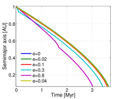
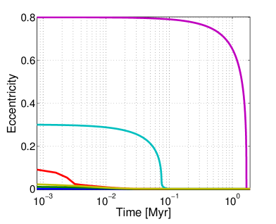
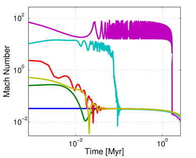
Figure 2.— Evolution of orbital elements of various orbits starting at $a=1AU$ and different eccentricities. The mass of the planetesimal considered here is $2\cdot 10^{25}g$. Top: Evolution of the semi-major axis. Middle: evolution of the eccentricity. Note logarithmic scale. Bottom: Evolution of the Mach number. Note logarithmic scale.

In the following we present the results of a single planetesimal evolution and effects of GDF on its evolution where various types of orbits and planetesimal masses are considered.

3.3.1 Eccentric orbits

On the top panel of figure 2 we see that all the simulated orbits evolve in a similar manner. This is mostly due to the rapid circularization of the orbits; as the orbits circularize the relative gas-planetesimal velocities decrease, with a corresponding decrease of the Mach number.

Eventually, their Mach number decreases to $\mathcal{M}\approx 1$, at which stage GDF is highly efficient, leading to a rapid loss of the angular momentum. The larger the initial eccentricity is, the longer it takes the orbit to reach the trans-sonic limit. Generally, the eccentricity damping time-scale given by Eq. (14) is compatible with simulations. Actually, Eq. (14) overestimates $\tau_{e}$. More rigorous derivation could determine $\tau_{e}$ more accurately.

We see that in most cases the planetesimals migrate within $3$ Myrs, compatible with the estimation of $\tau_{a}$ in (13). The greater the initial eccentricity of the orbit is, the faster it spirals in. This is due to the enhanced gas density $(\rho_{g}\propto a^{-16/7})$ in the apastron. For smaller planetesimals, e.g. of mass $\sim 10^{23}g$, $\tau_{a}$ increases to $\sim 200Myr$, much more than typical disk lifetimes. Note that given the short circularization time of eccentric orbits the time-scale for the evolution of the semi-major axis is almost independent of the initial eccentricity, and orbits with initial eccentricities of $e\lesssim 0.3$ are essentially circular through most of their orbital evolution.

Orbits with initial eccentricity of $e=0.1$ circularize to $\sim 0.02$ over $10^{4}$ years, and are fully circularized after $10^{5}$ years. For orbits of initial eccentricity $e=0.3,$ the circularization time extend to $\sim 0.1$Myrs. For smaller masses, the lowest mass for which the $\tau_{e}$ is comparable to typical disk lifetimes is $\sim 10^{23}g$, which corresponds to $500$km planetesimals. Less massive planetesimals hardly evolve within the disk lifetime.

3.3.2 Mildly inclined orbits

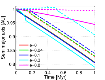
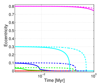
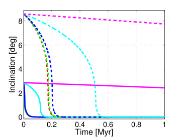
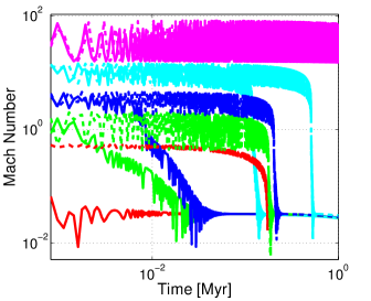
Figure 3.— The evolution of a $2\cdot 10^{25}g$ planetesimal over $1$Myr staring on inclined orbits. Solid lines correspond to orbits with initially low inclination $I=0.05$ rad, and dashed lines represent orbits with initially high inclination $I=0.15$ rad. Top left: Evolution of the semi-major axis. Top right: Evolution of the eccentricity. Note logarithmic scale. Bottom left: Evolution of the inclination. Bottom right: Evolution of the Mach number. Note logarithmic scale.

In figure 3 we show the results for initially inclined orbits. In the first three panels, orbits with low inclination show a fast decay.

The average ambient gas density experienced by planetesimals at high inclination is low compared with the low inclination orbits, hence GDF becomes less effective. Highly eccentric orbits, $e>0.3$, share the same fate. In special cases $(e=0.3,\ I=0.15$ rad, dashed cyan line) the orbit might gain angular momentum and expand, due to tailwind near the apastron that overcomes the headwind in periastron.

Figure 4.— Comparison of the orbital evolution of a $2\cdot 10^{25}g$ planetesimal for a range of initial conditions. Solid lines correspond to circular orbits, $e=0$. Dashed lines correspond to initially eccentric orbits $e=0.1$. The color index is green - $I=0$, red - low inclination $I\sim 2H_{0}$, blue - high inclination $I\sim 6H_{0}$. Top left: Evolution of the semi-major axis. Top right: Evolution of the eccentricity. Note logarithmic scale. Bottom left: Evolution of the inclination. Note logarithmic scale. Bottom right: Evolution of the Mach number. Note logarithmic scale.

For low inclination and circular orbit, the inclination drops sharply; a planetesimal on a circular orbit loses half its initial inclination already after a few Kyr, comparable to the estimated time-scale in Eq. 15. Orbits with high inclinations decay much slower, as expected.

In Fig. 4 we compare the evolution of inclined orbits with those obtained for zero inclination orbits. We consider inclinations in the range of $I=0-0.15$ rad, comparable with the disk aspect ratio $\sim 2H_{0},6H_{0}$, corresponding to gas density of $1\sigma$ and $3\sigma$ an the apastron/periastron respectively. The eccentricity is taken to be either $0$ or $0.1$. As can be seen in the first panel, the final decay time-scale $\tau_{a}$ is the same in all cases regardless of inclination and eccentricity, although for high inclination the decay is somewhat slower at first. On the second panel, we see that $\tau_{e}$ is different in each case. There is an order of magnitude difference between orbits with initial inclinations of $I=0$ and $I=0.05$ rad, and another order of magnitude difference compared with the initial $I=0.15$ rad case. Thus, $\tau_{e}$ is sensitive to inclination. In the third panel both the circular and eccentric orbit decay at the same phase for all inclinations, but the circular orbits always have lower inclination since the orbit is supersonic on the eccentric orbits and GDF is less efficient. Only after the eccentricity becomes negligible does $\tau_{i}$ retains its higher phase.

3.3.3 Highly inclined orbits

In the last section we considered low inclination orbits; however, observations of the Solar System and other dynamical systems show an ample of evidence for irregular orbits, with large and retrograde inclinations. In this sections we explore effects on GDF planetesimals in such high inclination orbits.

Consider for example circular prograde ($I=0$) and retrograde ($I=180^{\circ}$) orbits. In each case, the dimensionless force is $\mathcal{I}(\mathcal{M})/\mathcal{M}^{2}$. For prograde orbit, $\mathcal{M}_{prograde}\approx 0.033$ and $F_{prograde}=\mathcal{M}_{prograde}/3=0.011$, while for retrograde orbit, $\mathcal{M}_{retrograde}\approx 90$ and $F_{retrograde}\approx 10/90^{2}\approx 0.0012$, so $F_{prograde}/F_{retrograde}\approx 9$. We expect that the prograde orbit will decay nine times faster than retrograde orbit. In Fig. 5 we plot the evolution of the orbital elements of various initially inclined orbits. In the top left panel we see that after $1$ Myr, a planetesimal on a circular prograde orbit ($I=0$ deg, solid black line) has migrated by $\Delta a_{prograde}=0.17$AU, while the one on a retrograde orbit ($I=180$ deg, blue solid line) has migrated by $\Delta a_{retrograde}=0.02$AU, hence $\Delta a_{prograde}/\Delta a_{retrograde}\approx 0.17/0.02\approx 8.5$ , consistent with our expectations.

Figure 5.— Comparison between the evolution of planetesimals of $m=2\cdot 10^{25}g$ with various initial inclinations and eccentricities. Solid lines indicate circular orbits, dashed lines indicate eccentric orbits with initial eccentricity of $e=0.1$. Black, blue and green lines indicate initial inclination of $0,20$ and $180$ deg respectively. Top left: Evolution of the semi-major axis. Top right: evolution of orbital eccentricity. Note logarithmic scale. Bottom left: Evolution of Mach number. Note logarithmic scale. Bottom right: Evolution of inclination. We plot only orbits with initial inclinations of $20$ deg. The solid cyan line corresponds to an initially circular orbit, and the dashed magenta line corresponds to an eccentric orbit with initial eccentricity of $e=0.1$.

In the top right panel, only the planetesimal on a co-planar circular orbit (dashed black line) was able to circularize within $1$Myr of evolution. In the bottom left panel we only plot orbits wi th initial inclinations of $20$ deg, since both prograde and retrograde orbits are co-planar and do not change their inclination. We see that the changes in inclinations are mild. On the other hand, inclined orbits with inclination of $\sim 9$ deg lost their initial inclinations in less than a Myr. We conclude that orbits with inclinations higher than $I\gtrsim 4H_{0}\sim 12$ deg are not significantly affected by GDF.

3.3.4 Disk density profile

In the previous sections we considered disks with a disk density profile normalized with $\rho_{g}\sim a^{-9/7-\alpha}$ corresponding to a surface density profile of $\Sigma_{g}\sim a^{-\alpha}$ with $\alpha=1$. In the following we consider other disk profiles. In Fig. 6 we run simulations of co-planar orbits with eccentricity of either $0$ (solid line) or $0.1$ (dashed line). The power law density profiles considered are for $\alpha=1,1.5,2$, corresponding to the black, green and blue lines respectively. We have normalized the density profiles at $1$AU.

As can be seen in the top left panel, migration occurs more rapidly for larger $\alpha$; the time-scale for migration is shortened by factor of $\sim 3/2$ for $\alpha=1.5$ and $\sim 2$ for $\alpha=2$. The migration time-scale is insensitive to initial eccentricity, since circularization time-scale is rapid. The fast circularization is confirmed in the top right panel, where the eccentricity decays after few Kyrs. Bottom left panel shows the changes in semi-major axis for the first $10$Kyr. We see that after the initial fast decay of eccentric orbits, they start to decay in the same manner once they have been circularized. Only at later times there is difference due to different ambient density closer to the star. In the bottom right panel, the changes in Mach number are almost identical, consistent with the eccentricity decay in the top right panel. In the case of fixed normalization at $1$AU, $\tau_{a}$ decreases as the density profile is steeper, with virtually no effect to $\tau_{e}$ .

In Fig 7, we run co planar orbits with $\alpha=1,1.5,2$, initial eccentricities of $e=0.1,0.3,0.8$. This time, we normalize each density profile to $\rho_{0}$ at the periastron. On the top left panel we see that the more eccentric orbits decay slower since their ambient orbit averaged density is lower. Conversely to the previous case, orbits with different $\alpha$ migrate and circularize at a different phase.

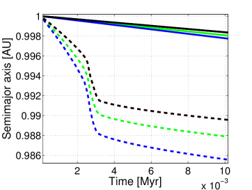
Figure 6.— Comparison between the evolution of planetesimals of $m=2\cdot 10^{25}g$ in protoplanetary disks with with different disk density profiles normalized at $1$AU. Solid lines indicate circular orbits, dashed lines indicate eccentric orbit with initial eccentricity of $e=0.1$. Black, blue and green lines indicate density profile $\Sigma_{g}\sim a^{-\alpha}$ where $\alpha$ is $1$, $1.5$ and $2$ respectively. Top left: Evolution of the semi-major axis. Top right: evolution of orbital eccentricity. Note logarithmic scale. Bottom left: Evolution of semi-major axis zoomed in on first $10^{4}$years. Bottom right: Evolution of Mach number. Note logarithmic scale.

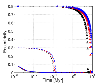
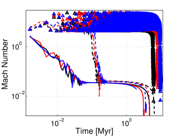
Figure 7.— Same as Fig. 6, but with normalization at the periastron. Top left: Evolution of the semi-major axis. Top right: evolution of orbital eccentricity. Note logarithmic scale. Bottom left: Evolution of semi-major axis zoomed in on first $10^{4}$years. Bottom right: Evolution of Mach number. Note logarithmic scale.

3.4. Scaling with planetesimal mass

Fig. 8 shows the dependence of the time-scales for the evolution of the orbital elements on the $\sim m_{p}^{-1}$ mass scaling. We consider time-scales comparable to the gas-disk lifetime of up to $10Myr$. The slowest evolution time-scale, $\tau_{a}$, is in found for semi-major axis; only planetesimals more massive than a few times $10^{24}g$ are significantly affected by GDF. The eccentricity damping is more rapid. The lower limit for the mass of planetesimals which are significantly affected (i.e. the damping time-scale of at least one of their orbital elements, $\tau_{a}$, $\tau_{e}$ or $\tau_{I}$, is comparable to the disk lifetime) is $m\approx 8\cdot 10^{21}g$ for $e=0.1$ and $m\approx 10^{23}g$ for $e=0.3$. Generally $\tau_{e}$ is an increasing function of $e$, but even for high eccentricity ($e\sim 0.8$), we still get $\tau_{e}\lesssim\tau_{a}$. The inclination time-scale, $\tau_{I}$, is by far the most rapid. For low inclination $I=0.05$ rad we have the lower limit $m\approx 4\cdot 10^{21}g$ . Generally $\tau_{I}$ is an increasing function both of initial inclination and eccentricity. For $I\sim 0.15$ $\tau_{I}$ is $\sim 100$ times slower , and starting with $e=0.1$ adds another order of magnitude to $\tau_{I}$.

Figure 8.— Dependence of the time-scales for orbital evolution obtained from numerical simulations. The shaded region is excluded due to gas dispersal after $10Myrs$. Solid line indicate semi-major axis evolution time-scale, $\tau_{a}$(blue). Dashed lines indicate eccentricity evolution rime scale, $\tau_{e}$, for $e=0.1$ (red) and $e=0.3$ (green). Triangles indicate the inclination evolution time-scale, $\tau_{I}$, for a circular orbit with initial $I=0.05$ rad. note logarithmic scales.

It is clear that for single IMPs, GDF damps both inclination and eccentricity efficiently for most mass ranges. Planetary embryos of mass $>10^{25}$g also migrate inward on time-scales of a few Myrs.

4. Discussion

Before exploring the implications of GDF for the evolution of planetesimal disks we discuss the various assumptions of which we made use as well as potential caveats in the approach taken here. We then also compare the effects of GDF to formulation of type I planetary migration. Finally we discuss the potential role of GDF in the evolution of protoplanetary disks.

4.1. Validity of assumptions and caveats

Accretion:

We have shown in section 3.1 that gas accretion is negligible for planetesimal radius $R\lesssim 1000$km. In section 2 we have shown that gas drag is negligible for $R\lesssim 500$km. Thus, for intermediate mass planetesimals both gas drag and accretion are negligible. This intermediate regime therefore complements Lee & Stahler (2011)’s analysis, where the dominant force considered was due to accretion. For larger radii and fully formed planets accretion is the dominant force and one should use models with accretion as the dominant drag force (e.g. Lee & Stahler, 2011, Lee & Stahler, 2014).

Linear regime:

Kim (2010) has studied the non-linear regime of GDF. The non-linearity parameter is

$$\mathcal{B}=\frac{Gm_{p}}{c_{s}^{2}R(\mathcal{M}^{2}-1)}=\frac{r_{B}}{2R(\mathcal{M}^{2}-1)}$$

For low Mach numbers it reduces to the condition for accretion. Hence we conclude that for planetesimals of radius $R\lesssim 1000$km the linear regime considered here is applicable. For larger embryos non-linear effects are non-negligible, where non-linear effects tend to decrease the GDF force by a factor of a few (Kim, 2010).

Time dependent 3D geometry vs. steady state 2D geometry:

Ostriker (1999)’s original derivation made use of time dependent perturbation theory, where the perturbation is turned on at time $t=0$. In a time dependent analysis there is a non-zero force in the subsonic regime, however the surprising result is that this force is time independent. The reason is that contributions from large distances (the far field) are not negligible. However, for disks, the emitted sound waves eventually reach the vertical edge $h$ of the disk after time $t\sim h/c_{s}=1/\Omega\sim 1$yr. Hence, after one orbital period the waves cannot propagate further and the contribution from the far field decreases until it becomes negligible.

In order to tackle the problem, Muto et al. (2011) solved the equations of motion in a slab geometry. They introduced an averaged potential at the scale height of the disk, i.e. $\Psi=-Gm_{p}/\sqrt{x^{2}+y^{2}+(\gamma h)^{2}}$ where $\gamma$ is of order unity factor. They decomposed the solution into Fourier components and searched for steady state solutions. Moreover, they showed that time dependent solutions decay as $\sim t^{-1}$, and therefore after $t\sim 1$yr the wake persists in a steady state.

Nevertheless, such a steady state might never be reached. Muto et al. (2011) note that the assumption for a steady state is only marginally satisfied. Moreover, there is uncertainty in the 2D approximation, and the force might be altered by a factor of a few. In addition, protoplanetary disks tend to be turbulent, which may significantly affect the perturbation evolution. The turbulence is parametrized by the turbulent viscosity $\nu=\alpha c_{s}h$ where $\alpha$ is the Shakura-Sunyaev parameter (Shakura & Sunyaev, 1973), not to be confused with disk density scaling power law. Consider a Kolmogorov distribution, i.e. the flow consists of self-similar eddies, and energy cascades from the largest eddy to the smallest one, where it is dissipated by molecular viscosity (Chiang & Youdin, 2010). In this case, the largest eddies are of order $l_{0}\sim h$, and the eddy turnover time-scale is $t_{0}=l_{0}/v_{0}=1/\Omega$. where $v_{0}\sim c_{s}$ is the velocity of the largest eddy. After a few $t_{0}$, the gas is well mixed and the density wave starts to propagate again from the planetesimal outwards. This is equivalent, in some sense, to restarting the problem. Since $t_{0}\lesssim 1/\Omega$, the steady state might not be reached, and the pressure wave propagation is restarted every few$\times$ $t_{0}$.

For smaller eddies, the characteristic eddy turnover time is $t_{l}\sim(l/l_{0})^{2/3}t_{0}$. Thus, for a wake with characteristic length $l=c_{s}t$, the relevant turnover time-scale corresponding to its length is $t_{l}/t=(\Omega t)^{-1/3}$. For $t\ll 1/\Omega$, the perturbation is not affected by the eddy current, and only for $t\sim 1/\Omega$ the turbulent current of the largest eddy destroys the wake, and one therefore needs to consider a time-dependent evolution following Ostriker.

Another possible reason for the steady state not being reached is that the planetesimals come back to (nearly) the original position after one orbit. For subsonic regime the gas has enough time to rearrange itself, but for super-sonic regime subsequent perturbations of the disk are possible. Kim & Kim (2007) find the number of interactions with the wake increases monotonically with larger Mach numbers.

Another attractive feature in Ostriker (1999)’s linear theory, is that it does not deal with viscosity and dissipation, which would affect the model studied by Muto et al. (2011), since these are second order effects. Our approach is therefore complimentary and consider the time dependent approach following Ostriker.

If $\alpha$ is low, and the disk is laminar, we can compare between both models. Denoting the GDF forces Ostriker (1999)’s 3D model and Muto et al. (2011)’s 2D model as

$$F_{3}(\mathcal{M})=F_{0}\mathcal{I}(\mathcal{M})$$ (16)

and

$$F_{2}(\mathcal{M},\alpha)=F_{0}\left\{\begin{array}[]{cc}\alpha/8&\mathcal{M}<1\\ F_{0}/2&\mathcal{M}>1\end{array}\right.$$

respectively, where $F_{0}=4\pi G^{2}m_{p}^{2}\rho_{g}/v_{rel}^{2}$ (see Eqs. (30) and (41) in Muto et al., 2011 for details). We estimate the ratio between both models

$$\frac{F_{3}}{F_{2}}=\left\{\begin{array}[]{cc}\frac{8}{3\alpha}&\mathcal{M}<1\\ 2\ln\frac{Vt}{r_{min}}+\ln(1-\mathcal{M}^{-2})&\mathcal{M}>1\end{array}\right.$$

For a subsonic perturber, with $\alpha\sim 10^{-2}$, the difference is 2-3 orders of magnitude. The situation gets better for supersonic perturber, where the second term is negligible, and the difference is $\sim 2\ln Vt/r_{min}$. The Coulomb logarithm is not well defined, but here $\ln\Lambda\sim\ln h(a)/r_{min}\sim 9-10$, so the difference becomes smaller, only one order of magnitude. We simulated planetesimals of $2\cdot 10^{25}g$, or with radius of $1000km$. The minimal radius is the minimum of either the physical radius of the planetesimal, the Bondi radius or the non-linearity radius. For IMPs $r_{min}$ is the physical size the planetesimal, of the order of $1000$km. The two models are therefore marginally compatible in supersonic regime, where as a much more significant difference is expected in the subsonic regime.

Shear:

The derivation for linear regime is valid for homogeneous gas. In reality, Keplerian disks have differential shear. Muto et al. (2011) suggest that the shear is negligible if the distance from the planet’s semi-major axis to the instantaneous co-rotation radius, defined by $a_{C}=a(1-e)/(1+e)$ is larger the the relevant length scale, i.e. $|a_{C}-a|\gtrsim h$, or $e\gtrsim 2H_{0}$. However, they neglected the pressure gradients since they were initially interested in supersonic orbits. In our case, for circular orbit spiral density wave appears where the relative velocity is supersonic and the effective Lindblad resonances accumulate (Artymowicz, 1993), so the morphology of the wave will be distorted on scales comparable to the scale height $\sim H_{0}a=h$. The overall force will therefore potentially differ by a factor of a few.

4.2. Connection to type I migration

In section 2 we have compared between aerodynamic gas drag and GDF. As mentioned earlier, these forces originate from essentially different physical processes. Aerodynamical gas drag originates from difference in the pressure due to changes in the flow around the body. It is proportional to the area and depends on geometry. GDF, on the other hand originates from gravitational interactions between the massive body and the ambient gas, and proportional to the mass (squared) of the body. Aerodynamical gas drag acceleration decreases with increasing mass, while GDF acceleration increases with increasing mass. The comparison between gas drag and GDF is straightforward.

In the case of GDF and type I migration, however, the comparison and the connections are less trivial. Both approaches deal with gravitational interactions between the planetesimal and the gaseous disk.

Up to dimensionless factors, the GDF torque is

$$T_{gdf}\sim a\frac{G^{2}m_{p}^{2}\rho_{g}}{c_{s}^{2}}$$

while the type I migration torque (e.g. Armitage, 2013; Tanaka et al., 2002) is

$$T_{migration}\sim\Sigma_{g}\Omega^{2}a^{4}\left(\frac{m_{p}}{M_{\star}}\right)^{2}\left(\frac{h}{a}\right)^{-2}$$ (17)

Where $\Sigma_{g}=2\rho_{g}h$ is the gas surface density. Both torques depend on the planetesimal mass and disk parameters on the same way. The ratio between both torques is $T_{GDF}/T_{migration}\sim(h/a)^{-1}$. The factor $h/a$ comes from the fact that the differential torque scales with $h/a$ (Ward, 1986). This is because there is an intrinsic asymmetry between inner and outer torques. In some sense, this is analogous to tidal forces that rise due to asymmetry of the gravitational forces induced on a solid body. One can better see the relation between these approaches by estimating the one sided torque using the GDF formulation, where the relevant relative velocity is the sound speed and the relevant formula is the supersonic one since effective Lindblad resonances resides at locations where the relative velocity between the flow and the planetesimal is equal to the sound speed (Artymowicz, 1993).

Finally, in our study we consider disk-planetesimal interactions on eccentric orbits. Note that the effect of eccentricity on planet migration was discussed in several studies such as Papaloizou & Larwood, 2000. They find that for eccentricity larger than $\sim\leavevmode\nobreak\ 1.1H_{0}$ the torque reverses. It has been confirmed by Cresswell et al. (2007) and Bitsch & Kley (2010), but the embedded planet is always migrating inward. The reason is that the torque changes the eccentricity, while the migration rate is calculated from the power, which is always negative for isothermal disks. In our models we always see inward migration.

4.3. Implications of gas dynamical friction for planet formation and the evolution of protoplanetary disks

Planetesimal disk evolution: When considering the evolution of large and small planetesimals in a disk, the evolution of the velocity dispersion is governed by viscous heating of the large bodies by themselves and their cooling by dynamical friction, whereas small planetesimals mostly heat through dynamical friction by the large bodies (Goldreich et al., 2002). Introducing gas to the system gives rise to additional cooling channels both for large and small bodies. For large oligarchs, GDF keeps the random velocities low, which prevents oligarch collisions. For small bodies, aerodynamic gas drag is the main process which dominates their cooling; such cooling is more than two order of magnitudes faster than cooling of small planetesimals through inelastic collisions (Goldreich et al., 2002) considered before. Moreover, the drag force increases with increasing velocity, so any random velocity raised by viscous stirring will be suppressed by gas drag. GDF therefore keeps planetesimal disks thin and cool much longer than otherwise thought, and can not be neglected.

For the upper tail of large ptotoplanets, the mass is close to the isolation mass $M_{iso}\sim 0.07M_{\oplus}(a/AU)^{3}(\Sigma_{g}/10g\cdot cm^{-3})^{3/2}$ where the protoplanet has cleared its feeding zone (Pollack et al., 1996). A large protoplanet under GDF force could migrate to a new environment where additional-planetesimal swarms are available for accretion. Hence the protoplanets do not grow in isolation and its growth is not limited by its local feeding zone.

Higher relative velocities can also affect the embryonic migration rate and eccentricity and inclination damping. While initially eccentric orbit is rapidly circularized in disks around single stars, planetesimals embedded in disks of binary stellar systems can have persistent higher relative velocities. The origin of high relative velocity can be either eccentric co-planar disk, or inclined orbit due to misaligned stellar companion (Rafikov & Silsbee, 2015).

Super-Earth / hot Neptune formation:

The observed distributions of planets in short periods suggest that lower mass super-Earths / hot Neptunes are more common than gas giants, compared with simple expectations from population synthesis models (Ida & Lin, 2008; Hansen & Murray, 2012). In order to reproduce the observed mass distribution an over-abundance of rocky material is required in the inner ($<1$AU) region. This can be achieved either by radial drift of rocky material in the form of dust or small planetesimals (Hansen & Murray, 2012), or by enhanced primordial minimal mass extrasolar nebula (MMEN) surface density profile (Chiang & Laughlin, 2013). Other suggestions involve type I migration of planets formed in the outer region into the inner region, which requires additional physical processes to concede with observations (i.e. eccentricity damping, tidal friction, pressure maxima trapping, Inamdar & Schlichting, 2014). Both suggestions suffer from theoretical and observational challenges: migration of small planetesimals through aerodynamic gas-drag, might be too fast and lead to the accretion of the solid material by the star, while enhanced primordial MMEN is unlikely and might be unstable (Inamdar & Schlichting, 2014). Migrating embryos due to GDF could provide an additional channel for supply of solid material into the inner region in the form of intermediate size planetesimal/planetary-embryos. GDF embryonic migration naturally introduces eccentricity damping, and thus alleviates the need for external mechanisms for eccentricity damping. Moreover, slightly eccentric orbit results in a more efficient migration, hence the migration starts at the scale of intermediate size planetesimals. In addition, for a configuration of eccentric disk in binary star system, higher relative velocity are predominant for the entire disk lifetime, and the embryonic migration rate might be faster and cause even more favorable conditions for generating super-Earths in circumbinary disks.

These embryos could therefore assist in providing the required over-abundance of rocky material for in-situ formation of hot Neptunes. In addition, the time-scales involved are comparable with disk lifetime, hence the migration is not too efficient as to lead to material accretion into the star, but its time-scales are sufficiently short as to supply the material during the lifetime of the gaseous disk.

5. Summary

In this study we considered the effect of GDF on single IMPs. We find that GDF is the dominant drag force affecting the evolution of planetesimals larger than $10^{21}g$, for which aerodynamic gas drag effects are negligible. We explored the effect of GDF in the linear regime and in the mass range where accretion and non linear effects are negligible (up to $\sim 10^{25}g$). We estimated the typical time-scales for the evolution of the orbital parameters of the planetesimals due to GDF, and further studied them using detailed numerical simulations. The main results can be summarized as follows.

Planetary embryos of mass $10^{24}-10^{25}g$ dissipate their inclinations and circularize in less than a Myr, regardless of initial parameters. Moreover, they migrate inward on time-scales comparable to the gaseous disk lifetime $\sim 5Myr$. Such embryonic migration may help explain the origin of close-in super-Earth planets, that might form and grow in the inner parts of the protoplanetary disk from such embryos (see also Hansen & Murray, 2012, for related issues). Smaller planetesimals ( $m\sim 10^{23}g$) may dissipate low initial eccentricities/inclinations ($e_{0}\lesssim 0.3$, $I_{0}\lesssim 0.1$rad). Planetesimals in the lowest mass range $(\sim 10^{21}g)$ can dissipate low initial eccentricities $(e_{0}\lesssim 0.1)$, and slightly damp small inclinations (comparable to the disk scale height). The efficient damping of inclination and eccentricity reduces the planetesimal random velocities and assist in keeping the planetesimal disk flatter and more circular, exchanging the planetesimals kinetic energy into the gaseous disk. Such evolution could therefore have implication not only for the planetesimal disk structure but also for the long term collisional evolution and planetary growth in the disk. We conclude that GDF can play an important role in the evolution of planetesimal disk, and should be accounted for in the study of the early stages of planet formation.

Appendix A A. TYPICAL ECCENTRICITY IN THE TRANS-SONIC REGIME

We wish to estimate the critical eccentricity $e_{c}$ for trans-sonic regime. The calculation is similar to Muto et al. (2011), where they neglect the pressure gradients of the gas and assume $\eta=0$. The relative velocities in polar coordinates are

$$v_{rel,r} = v_{r,gas}-v_{r}=-\frac{\Omega a}{\sqrt{1-e^{2}}}e\sin f$$ (A1)

$$v_{rel,\phi} = v_{\phi,gas}-v_{\phi}=\sqrt{1-\eta}\Omega a-\frac{\Omega a}{\sqrt{1-e^{2}}}(1+e\cos f)=\Omega a\left[\sqrt{1-\eta}-\frac{(1+e\cos f)}{\sqrt{1-e^{2}}}\right]$$ (A2)

The implicit assumption in obtaining (A1) and (A2) is that the large planetesimals are unaffected by GDF on a scale of orbital period. More formally, the stopping time is large compared to the orbital period. Indeed, (A1) and (A2) at zero eccentricity are obtained by letting $t_{s}\Omega\gg 1$ in Eqs. (16) and (17) in Perets & Murray-Clay (2011) and taking the first order.

The total relative velocity is

$$v_{rel}^{2} = v_{rel,r}^{2}+v_{rel,\varphi}^{2}=\frac{\widetilde{a}(e,\eta)+\widetilde{b}(e,\eta)\cos f}{1-e^{2}}v_{K}^{2}$$ (A3)

Where $\widetilde{a}(e,\eta)\equiv 2-\eta+{\eta}e^{2}-2(1-\eta)^{1/2}(1-e^{2})^{1/2}$ and $\widetilde{b}(e,\eta)\equiv 2e-2e\boldsymbol{(}1-\eta)^{1/2}({1-e^{2}})^{1/2}$. Note that $\widetilde{a}$ is a dimensionless quantity, not to be confused with the semi-major axis $a$. In order to acquire the average relative velocity, we need to average Eq. (A3) on one orbital period:

$$\langle v_{rel}^{2}(f(t),e,\eta)\rangle\equiv\frac{\Omega}{2\pi}\intop_{0}^{1/\Omega}v_{rel}^{2}(f,e,\eta)dt=\frac{\Omega}{2\pi}\intop_{0}^{2\pi}v_{rel}^{2}(f,e,\eta)\frac{dt}{df}df$$

Where $dt/df=a(1-e^{2})^{3/2}/(v_{K}(1+e\cos f)^{2})$. The average velocity is

$$\langle v_{rel}^{2}(e)\rangle = \frac{\sqrt{1-e^{2}}}{2\pi}v_{K}^{2}\left[\widetilde{a}\intop_{0}^{2\pi}\frac{df}{(1+e\cos f)^{2}}+\widetilde{b}\intop_{0}^{2\pi}\frac{\cos f}{(1+e\cos f)^{2}}df\right]$$

Which can be rewritten as

$$\langle v_{rel}^{2}(e)\rangle=v_{K}^{2}(1-e^{2})^{3/2}(2-\eta-2\sqrt{1-\eta}\sqrt{1-e^{2}})\frac{1}{2\pi}\intop_{0}^{2\pi}\frac{df}{(1+e\cos f)^{2}}$$ (A4)

Expanding in powers of $e$ we get

$$\langle v_{rel}(e)\rangle=v_{K}\left[(1-\sqrt{1-\eta})^{2}+\sqrt{1-\eta}e^{2}+O(e^{4})\right]^{1/2}$$ (A5)

For very low eccentricities $e\ll\varepsilon$, we get $\langle v_{rel}(e)\rangle=\varepsilon v_{K}$. For higher eccentricities $e\gg\varepsilon$ we get $v_{rel}\approx ev_{K}$. The critical eccentricity $e_{c}$ for which the flow is trans-sonic is $e_{c}\approx 2H_{0}=0.044$, consistent with Muto et al. (2011).

Appendix B B. NUMERICAL SET UP

At each step we first evaluate $c_{s}=0.022\cdot a^{2/7}$ and $\rho_{g}=1.7\cdot 10^{-3}$ at $1$AU in simulation units. For most runs we model the gas density with a power-law slope of $\rho_{g}\sim a^{-16/7}$ . Steeper slopes are considered in Section 3.3.4. Next, we evaluate $\eta=19/7(c_{s}/v_{K})^{2}$ and the Cartesian representation of the gas velocity $v_{x,gas}=-v_{r,gas}\sin f=-(1-\eta)^{1/2}v_{K}y/a$ as well as $v_{y,gas}=v_{r,gas}\cos f=(1-\eta)^{1/2}v_{k}x/a$, where $f$ is the true anomaly. Finally, we evaluate $\boldsymbol{v}_{rel}=\boldsymbol{v}_{p}-\boldsymbol{v}_{gas}$ , the scalar $v_{rel}=|\boldsymbol{v}_{rel}|$, and compute the Mach number by $\mathcal{M}=v_{rel}/c_{s}.$

The GDF coefficient $C_{GDF}$ which is calculated for every case is $4\pi\rho_{g}\mathcal{I}(\mathcal{M})$ where $\mathcal{I}(\mathcal{M})$ is $0.5\ln\left((1+\mathcal{M})/(1-\mathcal{M})\right)-\mathcal{M})$ in the subsonic regime, and $\ln\Lambda+0.5\ln(1-\mathcal{M}^{-2})$ in the supersonic regime. The effective Coulomb logarithm is $\ln\Lambda=\ln c_{s}t/R_{min}$. Taking $t=1yr$ and $R_{min}$ to be the planetesimal size, we get a Coulomb logarithm of the order of $10$. In a small interval near $\mathcal{M\sim}1$ we set $\mathcal{I}(\mathcal{M})=10$ to avoid singularity and make GDF function continuous.

The GDF coefficient is inserted into the acceleration per unit mass $\boldsymbol{da}=C_{GDF}\boldsymbol{v}_{rel}/v_{rel}^{3}$ and jerk per unit mass

$$\boldsymbol{dj} = \frac{d}{dt}\left(C_{GDF}\cdot\frac{\boldsymbol{v}_{rel}}{v_{rel}^{3}}\right)$$

$$= \frac{4\pi\rho_{g}}{v_{rel}^{3}}\left[\frac{(\boldsymbol{v}_{rel}\cdot\boldsymbol{da})}{v_{rel}}\boldsymbol{v}_{rel}\left(\frac{1}{c_{s}}\frac{d\mathcal{I}(\mathcal{M})}{d\mathcal{M}}-\frac{3}{v_{rel}}\mathcal{I}(\mathcal{M})\right)+\mathcal{I}(\mathcal{M})\boldsymbol{da}\right]$$

where $d\mathcal{I}(\mathcal{M})/d\mathcal{M}$ is $\mathcal{M}^{2}/(1-\mathcal{M}^{2})$ in the subsonic regime and $-2/(\mathcal{M}(1-\mathcal{M}^{2}))$ in the supersonic regime.

The total acceleration and jerk are $\boldsymbol{a}=-m_{p}\boldsymbol{da}$ and $\boldsymbol{j}=-m_{p}\boldsymbol{dj}$ respectively.

References

- Armitage (2013) Armitage, P. J. 2013, Astrophysics of Planet Formation
- Artymowicz (1993) Artymowicz, P. 1993, ApJ, 419, 155
- Baruteau et al. (2011) Baruteau, C., Cuadra, J., & Lin, D. N. C. 2011, ApJ, 726, 28
- Bitsch & Kley (2010) Bitsch, B., & Kley, W. 2010, A&A, 523, A30
- Bondi, H. (1952) Bondi, H. 1952, Monthly Notices of the Royal Astronomical Society, 112, 195
- Brown & Lawyer (2003) Brown, P., & Lawyer, D. 2003, J. Environ. Eng., 129, 222
- Cantó et al. (2013) Cant , J., Esquivel, A., S nchez-Salcedo, F. J., & Raga, A. C. 2013, ApJ, 762, 21
- Chiang & Laughlin (2013) Chiang, E., & Laughlin, G. 2013, MNRAS, 431, 3444
- Chiang & Youdin (2010) Chiang, E., & Youdin, A. N. 2010, Annual Review of Earth and Planetary Sciences, 38, 493
- Chiang & Goldreich (1997) Chiang, E. I., & Goldreich, P. 1997, ApJ, 490, 368
- Cresswell et al. (2007) Cresswell, P., Dirksen, G., Kley, W., & Nelson, R. P. 2007, A&A, 473, 329
- Cuzzi et al. (2001) Cuzzi, J. N., Hogan, R. C., Paque, J. M., & Dobrovolskis, A. R. 2001, ApJ, 546, 496
- Escala et al. (2004a) Escala, A., Larson, R. B., Coppi, P. S., & Mardones, D. 2004a, Coevolution of Black Holes and Galaxies, 13
- Escala et al. (2004b) —. 2004b, ApJ, 607, 765
- Goldreich et al. (2002) Goldreich, P., Lithwick, Y., & Sari, R. 2002, nat, 420, 643
- Goldreich et al. (2004) —. 2004, araa, 42, 549
- Hansen & Murray (2012) Hansen, B. M. S., & Murray, N. 2012, ApJ, 751, 158
- Hourigan & Ward (1984) Hourigan, K., & Ward, W. R. 1984, Icarus, 60, 29
- Hut et al. (1995) Hut, P., Makino, J., & McMillan, S. 1995, ApJ, 443, L93
- Ida & Lin (2008) Ida, S., & Lin, D. N. C. 2008, ApJ, 685, 584
- Inamdar & Schlichting (2014) Inamdar, N. K., & Schlichting, H. E. 2014, ArXiv e-prints, arXiv:1412.4440
- Kim & Kim (2007) Kim, H., & Kim, W.-T. 2007, ApJ, 665, 432
- Kim & Kim (2009) —. 2009, ApJ, 703, 1278
- Kim et al. (2008) Kim, H., Kim, W.-T., & S nchez-Salcedo, F. J. 2008, ApJ, 679, L33
- Kim (2010) Kim, W.-T. 2010, ApJ, 725, 1069
- Lee & Stahler (2011) Lee, A. T., & Stahler, S. W. 2011, MNRAS, 416, 3177
- Lee & Stahler (2014) —. 2014, A&A, 561, A84
- Murray & Dermott (1999) Murray, C. D., & Dermott, S. F. 1999, Solar system dynamics
- Muto et al. (2011) Muto, T., Takeuchi, T., & Ida, S. 2011, ApJ, 737, 37
- Ohtsuki et al. (2002) Ohtsuki, K., Stewart, G. R., & Ida, S. 2002, Icarus, 155, 436
- Ormel & Klahr (2010) Ormel, C. W., & Klahr, H. H. 2010, A&A, 520, A43
- Ostriker (1999) Ostriker, E. 1999, ApJ, 513, 252
- Papaloizou & Larwood (2000) Papaloizou, J. C. B., & Larwood, J. D. 2000, MNRAS, 315, 823
- Papaloizou & Terquem (2006) Papaloizou, J. C. B., & Terquem, C. 2006, Reports on Progress in Physics, 69, 119
- Perets & Murray-Clay (2011) Perets, H. B., & Murray-Clay, R. A. 2011, ApJ, 733, 56
- Pfalzner et al. (2014) Pfalzner, S., Steinhausen, M., & Menten, K. 2014, ApJ, 793, L34
- Pollack et al. (1996) Pollack, J. B., Hubickyj, O., Bodenheimer, P., et al. 1996, Icarus, 124, 62
- Rafikov & Silsbee (2015) Rafikov, R. R., & Silsbee, K. 2015, ApJ, 798, 69
- Rein (2012) Rein, H. 2012, MNRAS, 422, 3611
- Sánchez-Salcedo & Brandenburg (1999) S nchez-Salcedo, F. J., & Brandenburg, A. 1999, ApJ, 522, L35
- Sánchez-Salcedo & Brandenburg (2001) —. 2001, MNRAS, 322, 67
- Shakura & Sunyaev (1973) Shakura, N. I., & Sunyaev, R. A. 1973, A&A, 24, 337
- Stahler (2010) Stahler, S. W. 2010, MNRAS, 402, 1758
- Tanaka & Ida (1999) Tanaka, H., & Ida, S. 1999, Icarus, 139, 350
- Tanaka et al. (2002) Tanaka, H., Takeuchi, T., & Ward, W. R. 2002, ApJ, 565, 1257
- Tanaka & Ward (2004) Tanaka, H., & Ward, W. R. 2004, ApJ, 602, 388
- Teyssandier et al. (2013) Teyssandier, J., Terquem, C., & Papaloizou, J. C. B. 2013, MNRAS, 428, 658
- Ward (1986) Ward, W. R. 1986, Icarus, 67, 164
- Youdin (2010) Youdin, A. N. 2010, in EAS Publications Series, Vol. 41, EAS Publications Series, ed. T. Montmerle, D. Ehrenreich, & A.-M. Lagrange, 187–207