Spin and Chirality Effects in Antler-Topology Processes at High Energy $e^{+}e^{-}$ Colliders

Abstract

We perform a model-independent investigation of spin and chirality correlation effects in the antler-topology processes $e^{+}e^{-}\to\mathcal{P}^{+}\mathcal{P}^{-}\to(\ell^{+}\mathcal{D}^{0})(\ell^{-}\mathcal{\bar{D}}^{0})$ at high energy $e^{+}e^{-}$ colliders with polarized beams. Generally the production process $e^{+}e^{-}\to\mathcal{P}^{+}\mathcal{P}^{-}$ can occur not only through the $s$-channel exchange of vector bosons, $\mathcal{V}^{0}$, including the neutral Standard Model (SM) gauge bosons, $\gamma$ and $Z$, but also through the $s$- and $t$-channel exchanges of new neutral states, $\mathcal{S}^{0}$ and $\mathcal{T}^{0}$, and the $u$-channel exchange of new doubly-charged states, $\mathcal{U}^{--}$. The general set of (non-chiral) three-point couplings of the new particles and leptons allowed in a renormalizable quantum field theory is considered. The general spin and chirality analysis is based on the threshold behavior of the excitation curves for $\mathcal{P}^{+}\mathcal{P}^{-}$ pair production in $e^{+}e^{-}$ collisions with longitudinal and transverse polarized beams, the angular distributions in the production process and also the production-decay angular correlations. In the first step, we present the observables in the helicity formalism. Subsequently, we show how a set of observables can be designed for determining the spins and chiral structures of the new particles without any model assumptions. Finally, taking into account a typical set of approximately chiral invariant scenarios, we demonstrate how the spin and chirality effects can be probed experimentally at a high energy $e^{+}e^{-}$ collider.

1 Introduction

The monumental discovery Aad:2012tfa ; Chatrchyan:2012ufa of the Higgs boson at the CERN Large Hadron Collider (LHC) has filled in the only missing piece of the SM of electroweak and strong interactions, completing its gauge symmetry structure and electroweak symmetry breaking (EWSB) through the so-called Brout-Englert-Higgs (BEH) mechanism Englert:1964et ; Higgs:1964ia ; Higgs:1964pj ; Higgs:1966ev ; Kibble:1967sv . Nevertheless, there are several compelling indications that the SM needs to be extended by including new particles and/or new types of interactions. Once any new particle indicating new physics beyond the SM is discovered at the LHC or high energy $e^{+}e^{-}$ colliders, one of the first crucial steps is to experimentally determine its spin as well as its mass because spin is one of the canonical characteristics of all particles required for defining a new theoretical framework as a Lorentz-invariant quantum field theory Wigner:1939cj .

Many models beyond the SM Wess:1974tw ; Nilles:1983ge ; Haber:1984rc ; Chung:2003fi ; Weinstein:1973gj ; Weinberg:1979bn ; Susskind:1978ms ; ArkaniHamed:1998nn ; Randall:1999ee ; Appelquist:2000nn ; ArkaniHamed:2001nc ; Csaki:2003dt ; Csaki:2003zu have been proposed and studied not only to resolve several conceptual issues like the gauge hierarchy problem but also to explain the dark matter (DM) composition of the Universe with new stable weakly interacting massive particles Griest:2000kj ; Bertone:2004pz ; Ade:2013zuv . For this purpose, a (discrete) symmetry such as $R$ paity in supersymmetric (SUSY) models and Kaluza-Klein (KK) parity in universal extra-dimension (UED) models is generally introduced to guarantee the stability of the particles and thus to explain the DM relic density quantitatively. As a consequence, the new particles can be produced only in pairs at high energy hadron or lepton colliders, leading to challenging signatures with at least two invisible final-state particles.

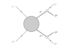
Figure 1: The correlated process $e^{+}e^{-}\rightarrow\mathcal{P}^{+}\mathcal{P}^{-}\rightarrow(\ell^{+}\mathcal{D}^{0})(\ell^{-}\mathcal{\bar{D}}^{0})$ characterized by the antler-topology diagram. Here, the invisible final-state particle $\mathcal{D}^{0}$ might be charge self-conjugate, i.e. $(\mathcal{D}^{0})^{c}=\mathcal{D}^{0}$.

At hadron colliders like the LHC such a signal with invisible particles is usually insufficiently constrained for full kinematic reconstructions, rendering the unambiguous and precise determination of the masses, spins and couplings of (new) particles produced in the intermediate or final stages challenging, even if conceptually possible, as demonstrated in many previous works on mass measurements Lester:1999tx ; Barr:2003rg ; Cho:2007qv ; Barr:2007hy ; Cho:2007dh ; Tovey:2008ui ; Cheng:2008hk ; Barr:2009jv ; Matchev:2009ad ; Polesello:2009rn ; Konar:2009wn ; Cohen:2010wv ; Alwall:2009sv ; Artoisenet:2010cn ; Alwall:2010cq ; Han:2009ss ; Han:2012nm ; Han:2012nr ; Swain:2014dha and on spin determination Barr:2004ze ; Smillie:2005ar ; Datta:2005zs ; Barr:2005dz ; Meade:2006dw ; Alves:2006df ; Athanasiou:2006ef ; Wang:2006hk ; Smillie:2006cd ; Choi:2006mt ; Kilic:2007zk ; Alves:2007xt ; Csaki:2007xm ; Wang:2008sw ; Burns:2008cp ; Cho:2008tj ; Gedalia:2009ym ; Ehrenfeld:2009rt ; Edelhauser:2010gb ; Horton:2010bg ; Cheng:2010yy ; Buckley:2010jv ; Chen:2010ek ; Chen:2011cya ; Nojiri:2011qn ; MoortgatPick:2011ix .

In contrast to hadron colliders, an $e^{+}e^{-}$ collider Behnke:2013xla ; Baer:2013cma ; Behnke:2013lya ; Koratzinos:2013chw ; Gomez-Ceballos:2013zzn ; Accomando:2004sz ; Linssen:2012hp has a fixed center-of-mass (c.m.) energy and c.m. frame and the collider can be equipped with longitudinally and/or transversely polarized beams. These characteristic features allow us to exploit several complementary techniques at $e^{+}e^{-}$ colliders for unambiguously determining the spins as well as the masses of new pairwise-produced particles, the invisible particles from the decays of the parent particles and the particles exchanged as intermediate states, with good precision. In the present work we focus on the following production-decay correlated processes

$$e^{+}e^{-}\,\to\,\mathcal{P}^{+}\mathcal{P}^{-}\,\to\,(\ell^{+}\mathcal{D}^{0})(\ell^{-}\mathcal{\bar{D}}^{0})$$ (1.1)

dubbed antler-topology events Han:2009ss , which contain the production of an electrically charged pair $\mathcal{P}^{+}\mathcal{P}^{-}$ in $e^{+}e^{-}$ collisions followed by the two-body decays, $\mathcal{P}^{+}\to\ell^{+}\mathcal{D}^{0}$ and $\mathcal{P}^{-}\to\ell^{-}\mathcal{\bar{D}}^{0}$, giving rise to a charged lepton pair $\ell^{\pm}(=e^{\pm},\mu^{\pm})$ and an invisible pair $\mathcal{D}^{0}\mathcal{\bar{D}}^{0}$ (See Fig. 1).

The invisible particle $\mathcal{D}^{0}$ may be charge self-conjugate, i.e. $\mathcal{\bar{D}}^{0}=\mathcal{D}^{0}$. Nevertheless, it is expected to be insubstantial quantitatively whether the particle is self-conjugate or not, unless the width of the parent particle $\mathcal{P}^{\pm}$ is very large and there exist large chirality mixing contributions Hagiwara:2005ym . So, any interference effects due to the charge self-conjugateness of the invisible particle will be ignored in the present work.

If the parent particle $\mathcal{P}^{-}$ carries an electron number $L_{e}(\mathcal{P}^{-})=+1$ or a muon number $L_{\mu}(\mathcal{P}^{-})=+1$, then the final-state leptons must be $e^{-}e^{+}$ or $\mu^{-}\mu^{+}$, respectively, if electron and muon numbers are conserved individually and the invisible particles, $\mathcal{D}^{0}$ and $\mathcal{\bar{D}}^{0}$, carry no lepton numbers. On the other hand, if the parent particle carries no lepton number, the final-state leptons can be any of the four combinations, $\{e^{-}e^{+},e^{-}\mu^{+},\mu^{-}e^{+},\mu^{-}\mu^{+}\}$, and the invisible particles, $\mathcal{D}^{0}$ and $\mathcal{\bar{D}}^{0}$, must carry the same lepton number as $\ell^{\mp}=e^{\mp},\mu^{\mp}$, respectively.

Once the masses of new particles are determined by (pure) kinematic effects Christensen:2014yya , a sequence of techniques increasing in complexity can be applied to determine the spins and chirality properties of particles in the correlated antler-topology process at $e^{+}e^{-}$ colliders Battaglia:2005zf ; Choi:2006mr ; Buckley:2007th ; Buckley:2008eb ; Boudjema:2009fz ; Christensen:2013sea :

• Rise of the excitation curve near threshold with polarized electron and positron beams;

• Angular distribution of the production process;

• Angular distributions of the decays of polarized particles;

• Angular correlations between decay products of two particles.

While the first and second steps (a) and (b) are already sufficient in the case with a spin-0 scalar $\mathcal{P}^{\pm}=S^{\pm}_{p}$ as will be demonstrated in detail, the production-decay correlations need to be considered for the case with a spin-1/2 fermion $\mathcal{P}^{\pm}=F^{\pm}_{p}$ and a spin-1 $\mathcal{P}^{\pm}=V^{\pm}_{p}$ to determine the $\mathcal{P}$ spin unambiguously; in principle a proper combination of these complementary techniques enables us to determine the spins of the invisible particles, $\mathcal{D}^{0}$ and $\mathcal{\bar{D}}^{0}$, and all the intermediate particles exchanged in $s$-, $t$- or $u$-channel diagrams participating in the production process. For our numerical analysis we follow the standard procedure. We show through detailed simulations how the theoretically predicted distributions can be reconstructed after including initial state QED radiation (ISR), beamstrahlung and width effects as well as typical kinematic cuts.

The paper is organized as follows. In Sect. 2 we describe a general theoretical framework for the spin and chiral effects in antler-topology processes at high energy $e^{+}e^{-}$ colliders. In Sect. 3 we present the complete amplitudes and polarized cross sections for the production process $e^{+}e^{-}\to\mathcal{P}^{+}\mathcal{P}^{-}$ in the $e^{+}e^{-}$ center-of-mass (c.m.) frame with the general set of couplings listed in Appendix A. The technical framework we have employed is the helicity formalism Jacob:1959at . Then, we present in Sect. 4 the complete helicity amplitudes of the two-body decays $\mathcal{P}^{+}\to\ell^{+}\mathcal{D}^{0}$ and $\mathcal{P}^{-}\to\ell^{-}\mathcal{\bar{D}}^{0}$ with general couplings given in Appendix A. Sect. 5 describes how to obtain the fully-correlated six-dimensional production-decay angular distributions by combining the production helicity amplitudes and the two two-body decay helicity amplitudes and by implementing arbitrary electron and positron polarizations Hikasa:1985qi ; Hagiwara:1985yu ; MoortgatPick:2005cw ; Choi:2006vh ; Ananthanarayan:2008dr . Sect. 6, the main part of the present work, is devoted to various observables: the threshold-excitation patterns, the production angle distributions equipped with polarized beams, the lepton decay polar-angle distributions and the lepton angular-correlations of the two two-decay modes. They provide us with powerful tests of the spin and chirality effects in the production-decay correlated process. While all the analytic results are maintained to be general, the numerical analyses are given for the theories with (approximate) electron chirality conservation such as SUSY and UED models and a subsection will be devoted to a brief discussion of the possible influence from electron chirality violation effects. Finally, we summarize our findings and conclude in Sect. 7. For completeness, we include three appendices in addition to Appendix A. In Appendix B, we list all of the Wigner $d$-functions used in the main text d functions:1957rs . In Appendix C, we describe how to obtain the expression of the production matrix element-squared for arbitrary polarized electron and positron beams. Finally, in Appendix D we give an analytic proof of the presence of a twofold discrete ambiguity in determining the $\mathcal{P}^{\pm}$ momenta in the process $e^{+}e^{-}\to\mathcal{P}^{+}\mathcal{P}^{-}\to(\ell^{+}\mathcal{D}^{0})(\ell^{-}\mathcal{\bar{D}}^{0})$, even if the masses of the particles, $\mathcal{P}^{\pm}$ and $\mathcal{D}^{0}$ ($\mathcal{\bar{D}}^{0}$), are a priori known.

2 Setup for model-independent spin determinations

Generally, the production part $e^{+}e^{-}\to\mathcal{P}^{+}\mathcal{P}^{-}$ of the antler-topology process (1.1) can occur through $s$-, $t$- and/or $u$-channel diagrams in renormalizable field theories, as shown in Fig. 2. Which types of diagrams are present and/or significant depend crucially on the nature of the new particles, $\mathcal{P}^{\pm}$, $\mathcal{D}^{0}$ and $\mathcal{\bar{D}}^{0}$ as well as the SM leptons $\ell^{\pm}$ and on the constraints from the discrete symmetries conserved in the theory.

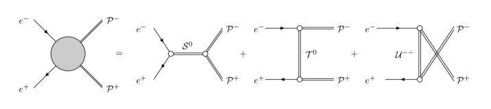
Figure 2: New $s$-channel $\mathcal{S}^{0}$-exchange diagrams (including the standard $\gamma$- and $Z$-exchange diagrams), new $t$-channel $\mathcal{T}^{0}$-exchange diagrams and new $u$-channel $\mathcal{U}^{--}$-exchange diagrams to the pair-production process $e^{+}e^{-}\to\mathcal{P}^{+}\mathcal{P}^{-}$.

We assume that the new particles, $\mathcal{P}^{\pm}$, $\mathcal{D}^{0}$ and $\mathcal{\bar{D}}^{0}$, are produced on-shell in the antler-topology process (1.1), and they are uncolored under the SM strong-interaction group so that they are not strongly interacting. Motivated mainly by the DM problem, the new particles are assumed to be odd under a conserved discrete $Z_{2}$-parity symmetry. Therefore, they can only be produced in pairs at high energy hadron and lepton colliders with an initial $Z_{2}$-parity even environment such as LHC, ILC, TLEP and CLIC, etc. Furthermore, the invisible particle $\mathcal{D}^{0}$ participating in the two-body decay $\mathcal{P}^{+}\to e^{+}\mathcal{D}^{0}$, if the decay mode is present, is included among the particles $\mathcal{T}^{0}$ exchanged in the $t$-channel diagram of the production process $e^{+}e^{-}\to\mathcal{P}^{+}\mathcal{P}^{-}$. This implies that unavoidably at least one of the particles $\mathcal{T}^{0}$ is lighter than the particle $\mathcal{P}^{\pm}$ in the antler-topology process with $\ell^{\pm}=e^{\pm}$.

As the $\mathcal{P}^{-}$ as well as the electron $e^{-}$ is singly electrically-charged, the $s$- and $t$-channel processes are mediated by (potentially several) neutral particles, $\mathcal{S}^{0}$ and $\mathcal{T}^{0}$, but any $u$-channel processes must be mediated by (potentially several) doubly-charged particles, $\mathcal{U}^{--}$. In passing, we note that most of the popular extensions of the SM such as supersymmetry (SUSY) and universal extra-dimension (UED) models contain no doubly-charged particles so that there exist only $s$-channel and/or $t$-channel exchange diagrams but no $u$-channel exchange diagrams contributing to the production process $e^{+}e^{-}\to\mathcal{P}^{+}\mathcal{P}^{-}$. The $s$-channel scalar-exchange contributions may be practically negligible as well because the electron-chirality violating couplings of any scalar to the electron line are strongly suppressed in proportion to the tiny electron mass in those SUSY and UED models.

Since the on-shell particles, $\mathcal{P}^{\pm}$, $\mathcal{D}^{0}$ and $\mathcal{\bar{D}}^{0}$ as well as the virtual intermediate particles, $\mathcal{S}^{0},\,\mathcal{T}^{0}$ and $\mathcal{U}^{\pm\pm}$, are not directly measured, their spins and couplings as well as masses are not a priori known. The neutral state $\mathcal{S}^{0}$ can be a spin-0 scalar, $S^{0}_{s}$, or a spin-1 vector boson, $V^{0}_{s}$, including the standard gauge bosons $V^{0}_{s}=\gamma,Z$ as well. Each of the other intermediate particles can be a spin-0 scalar, a spin-1/2 fermion or a spin-1 vector boson, assigned in relation to the spin of the particle $\mathcal{P}^{\pm}$. In any Lorentz-invariant theories, there exist in total twenty ($20=2+8+8+2$) different spin assignments for the production-decay correlated antler-topology process (1.1) as

$$\left(J_{\mathcal{P}},\!J_{\mathcal{D}};J_{\mathcal{S}},\!J_{\mathcal{T}},\!J_{\mathcal{U}}\right)\!=\!\bigg{\{}\!\left(0,\tfrac{1}{2};0\oplus 1,\tfrac{1}{2},\tfrac{1}{2}\right),\!\left(\tfrac{1}{2},0;0\oplus 1,0\oplus 1,0\oplus 1\right),\!\left(\tfrac{1}{2},1;0\oplus 1,0\oplus 1,0\oplus 1\right),\!\left(1,\tfrac{1}{2};0\oplus 1,\tfrac{1}{2},\tfrac{1}{2}\right)\!\bigg{\}}$$ (2.1)

with spins up to $1$ and couplings consistent with renormalizable interactions. The symbols used for the particles in our analysis are listed in Tab. 1 along with their charges, spins and $Z_{2}$ parities. Generically, the intermediate states, $\mathcal{S}^{0}$, $\mathcal{T}^{0}$ and $\mathcal{U}^{--}$ may stand for several different states, although typically the on-shell particle $\mathcal{P}^{\pm}$ or $\mathcal{D}^{0}$ stands for a single state. Note that, if the parent particle $\mathcal{P}^{\pm}$ turns out to be a spin-0 or spin-1 particle, then the daughter particles, $\mathcal{D}^{0}$ and $\mathcal{\bar{D}}^{0}$, and the $t$- and $u$-channel intermediate particles $\mathcal{T}^{0}$ and $\mathcal{U}^{\pm\pm}$ are guaranteed to be spin-1/2 particles.

Particle		Spin		Charge	$Z_{2}$ Parity
	$0$	$1/2$	$1$
$\ell^{-}$		$\ell^{-}$		$-1$	$+$
$\mathcal{D}^{0}$	$S^{0}_{d}$	$F^{0}_{d}$	$V^{0}_{d}$	$0$	$-$
$\mathcal{P}^{-}$	$S^{-}_{p}$	$F^{-}_{p}$	$V^{-}_{p}$	$-1$	$-$
$\mathcal{S}^{0}$	$S^{0}_{s}$	$F^{0}_{s}$	$V^{0}_{s}$	$0$	$+$
$\mathcal{T}^{0}$	$S^{0}_{t}$	$F^{0}_{t}$	$V^{0}_{t}$	$0$	$-$
$\mathcal{U}^{--}$	​ $S^{--}_{u}$	​ $F^{--}_{u}$	​ $V^{--}_{u}$	$-2$	$-$

Table 1: List of symbols used for the particles in our analysis with their electric charges, spins and $Z_{2}$ parities. The symbol $\ell^{-}$ denotes an electron $e^{-}$ or a muon $\mu^{-}$. The last three lines are for the new particles exchanged in the $s$-, $t$- and $u$-channel diagrams including the neutral electroweak gauge bosons, $\gamma$ and $Z$, exchanged in the $s$-channel diagram in the production process, $e^{+}e^{-}\to\mathcal{P}^{+}\mathcal{P}^{-}$.

Among the elementary particles discovered so far, the electron is the lightest electrically-charged particle in the SM. Its mass $m_{e}\simeq 0.51\,{\rm MeV}\,\sim 2\times 10^{-6}\,v$ is much smaller than the vacuum expectation value (vev) $v\simeq 246$ GeV of the SM Higgs field, the weak scale for setting the masses of leptons and quarks, as well as the c.m. energies of future high-energy $e^{+}e^{-}$ colliders. Any kinematic effects due to the electron mass are negligible so that the electron will be regarded as a massless particle from the kinematic point of view in the present work. The near masslessness of the electron is related to the approximate chiral symmetry of the SM. Any new theory beyond the SM should guarantee the experimentally-established smallness of the electron mass. This is a challenge in new theories beyond the SM since they usually involve larger mass scale(s) than the weak scale. One simple and natural protection mechanism is chiral symmetry.

Nevertheless, we do not impose any type of chiral symmetry so as to maintain full generality in our model-independent analysis of spin and chirality effects, emphasising the importance of checking experimentally to what extent the underlying theory possesses chiral symmetry. In each three-point vertex involving a fermion line, i.e. two spin-1/2 fermion states, we allow for an arbitrary linear combination of right-handed and left-handed couplings. Only in our numerical examples will every interaction vertex involving the initial $e^{\pm}$ line and the final-state lepton $\ell^{\pm}$ ($=e^{\pm},\mu^{\pm}$) be set to be purely chiral, as is nearly valid in typical SUSY and UED models, apart from tiny contaminations proportional to the electron or muon masses generated through the BEH mechanism of EWSB Englert:1964et ; Higgs:1964ia ; Higgs:1964pj ; Higgs:1966ev ; Kibble:1967sv .

3 Pair Production Processes

In this section we present the analytic form of helicity amplitudes for the production process

$$e^{-}(p_{-},\sigma_{-})\,+\,e^{+}(p_{+},\sigma_{+})\,\to\,\mathcal{P}^{-}(q_{-},\lambda_{-})\,+\,\mathcal{P}^{+}(q_{+},\lambda_{+})$$ (3.1)

with the $s$-, $t$- and $u$-channel contributions as depicted in Fig. 2 with the general three-point couplings listed in Appendix A. Here, we discuss only the amplitudes for on-shell $\mathcal{P}$ pair production. The technical framework for our analytic results is the standard helicity formalism Jacob:1959at .

The helicity of a massive particle is not a relativistically invariant quantity. It is invariant only for rotations or boosts along the particle’s momentum, as long as the momentum does not change its sign. In the present work, we define the helicities of the $\mathcal{P}^{\pm}$ in the $e^{+}e^{-}$ c.m. frame. Helicity amplitudes contain full information on the production process and enable us to take into account polarization of the initial $e^{+}e^{-}$ beams in a straightforward way as described in Appendix C.

Generically, ignoring the electron mass, we can cast the helicity amplitude into a compact form composed of two parts - an electron-chirality conserving (ECC) part $Q^{c}$ and an electron-chirality violating (ECV) part $Q^{v}$ - as

$${\cal M}[e^{-}_{\sigma_{-}}e^{+}_{\sigma_{+}}\to\mathcal{P}^{-}_{\lambda_{-}}\mathcal{P}^{+}_{\lambda_{+}}]=\sqrt{2}e^{2}\left[\,\delta_{\sigma_{+},-\sigma_{-}}Q^{c}_{\sigma_{-};\lambda_{-},\lambda_{+}}+\delta_{\sigma_{+},\sigma_{-}}Q^{v}_{\sigma_{-};\lambda_{-},\lambda_{+}}\right]\,d^{J_{0}}_{\Delta\sigma,\Delta\lambda}(\theta)$$ (3.2)

where $J_{0}={\rm max}(|\Delta\sigma|,|\Delta\lambda|)$ with the difference of the $e^{\mp}$ helicities $\Delta\sigma=J_{e}(\sigma_{-}-\sigma_{+})=\pm 1,0$ and that of the $\mathcal{P}^{\mp}$ helicities $\Delta\lambda=J_{\mathcal{P}}(\lambda_{-}-\lambda_{+})$. Here, $J_{e}=1/2$ and $J_{\mathcal{P}}$ are the spin of the electron and the particle $\mathcal{P}$, respectively. No helicity indices are needed when the spin of the particle $\mathcal{P}$ is zero, i.e. $J_{\mathcal{P}}=0$. After extracting the spin value of the electron and $\mathcal{P}$, $\sigma_{\pm}$ takes two values of $\pm 1$ while $\lambda_{\pm}$ takes two values of $\pm 1$ or three values $\pm 1,0$ for $J_{\mathcal{P}}=1/2$ or $1$, respectively. Frequently, in the present work we adopt the conventions, $\sigma_{-,+}=\pm$ and $\lambda_{-,+}=\pm,0$, will be used to denote the sign of the re-scaled helicity values for the sake of notational convenience. The angle $\theta$ in Eq. (3.2) denotes the scattering angle of $\mathcal{P}^{-}$ with respect to the $e^{-}$ direction in the $e^{+}e^{-}$ c.m. frame. The explicit form of the $d$ functions needed here is reproduced in Appendix B.

The polarization-weighted polar-angle differential cross sections of the production process can be cast into the form

$$\frac{d\sigma^{\mathcal{P}}_{\rm pol}}{d\cos\theta} = \frac{\pi\alpha^{2}\beta}{4s}\bigg{[}(1-P^{L}_{-}P^{L}_{+})(\mathcal{C}^{+}_{+}+\mathcal{C}^{-}_{-})+(P^{L}_{-}-P^{L}_{+})(\mathcal{C}^{+}_{+}-\mathcal{C}^{-}_{-})$$ (3.3)

$${}\hskip 8.5359pt\quad+(1+P^{L}_{-}P^{L}_{+})(\mathcal{V}^{+}_{+}+\mathcal{V}^{-}_{-})+(P^{L}_{-}+P^{L}_{+})(\mathcal{V}^{+}_{+}-\mathcal{V}^{-}_{-})$$

$${}\hskip 8.5359pt\quad+2P^{T}_{-}P^{T}_{+}\cos\delta\,{\rm Re}(\mathcal{V}^{-}_{+})+2P^{T}_{-}P^{T}_{+}\sin\delta\,{\rm Im}(\mathcal{V}^{-}_{+})\bigg{]}$$

with $\delta$ the relative opening angle of the electron and positron transverse polarizations and $\beta$ the speed of pair-produced particles, where $P_{\pm}^{L,T}$ is the degrees of longitudinal and transverse polarizations and $\delta$ is the relative opening angle of the $e^{\pm}$ transverse polarizations. The ECC and ECV production tensors $\mathcal{C}$ and $\mathcal{V}$ are defined in terms of the reduced production helicity amplitudes by

$$\mathcal{C}^{\sigma}_{\sigma} = \sum_{\lambda_{-},\lambda_{+}}\left|\,Q^{c}_{\sigma;\lambda_{-},\lambda_{+}}\right|^{2}\,\left[d^{J_{0}}_{\sigma,\Delta\lambda}(\theta)\right]^{2}$$ (3.4)

$$\mathcal{V}^{\sigma^{\prime}}_{\sigma} = \sum_{\lambda_{-},\lambda_{+}}\left(Q^{v}_{\sigma;\lambda_{-},\lambda_{+}}Q^{v*}_{\sigma^{\prime};\lambda_{-},\lambda_{+}}\right)\,\left[d^{J_{0}}_{0,\Delta\lambda}(\theta)\right]^{2}\,$$ (3.5)

with $\sigma,\sigma^{\prime}=\pm 1$ or simply $\pm$ for notational convenience. (For more detailed derivation of the polarized cross sections, see Appendix C.) The polarized total cross section $\sigma^{\mathcal{P}}_{\rm pol}$ can then be obtained by integrating the differential cross section over the full range of $\cos\theta$.

If all of the coupling coefficients are real and all the particle widths are neglected, the following relations must hold for both the ECC and ECV parts of the production helicity amplitudes:

$$Q^{c}_{\sigma;\lambda_{-},\lambda_{+}}=Q^{c*}_{\sigma;-\lambda_{+},-\lambda_{-}}\quad\mbox{and}\quad Q^{v}_{\sigma;\lambda_{-},\lambda_{+}}=Q^{v*}_{-\sigma;-\lambda_{+},-\lambda_{-}}$$ (3.6)

as a consequence of $CPT$ invariance in the absence of any absorptive parts. Therefore, violation of this relation indicates the presence of re-scattering effects. On the other hand, $CP$ invariance leads to the relation:

$$Q^{c}_{\sigma;\lambda_{-},\lambda_{+}}=Q^{c}_{\sigma;-\lambda_{+},-\lambda_{-}}\quad\mbox{and}\quad Q^{v}_{\sigma;\lambda_{-},\lambda_{+}}=Q^{v}_{-\sigma;-\lambda_{+},-\lambda_{-}}$$ (3.7)

independently of the absorptive parts so that the relation can be directly used as a test of CP conservation. Similarly, it is easy to see that P invariance leads to the relation for both the ECC and ECV amplitudes:

$$Q^{c,v}_{\sigma;\lambda_{-},\lambda_{+}}=Q^{c,v}_{-\sigma;-\lambda_{-},-\lambda_{+}}$$ (3.8)

which is violated usually through chiral interactions such as weak interactions in the SM.

Applying the $P$ and $CP$ symmetry relations to the ECC and ECV production tensors, (3.4) and (3.5), we can classify the six polar-angle distributions in Eq. (3.3) according to their $P$ and $CP$ properties as shown in Tab. 2. We find that the two combinations, $\mathcal{C}^{+}_{+}+\mathcal{C}^{-}_{-}$ and $\mathcal{V}^{+}_{+}+\mathcal{V}^{-}_{-}$, contributing to the unpolarized part are both $P$- and $CP$-even whereas the terms, $\mathcal{C}^{+}_{+}-\mathcal{C}^{-}_{-}$ and $\mathcal{V}^{+}_{+}-\mathcal{V}^{-}_{-}$, linear in the degrees of longitudinal polarization are $P$-odd and $CP$-even. One of the two transverse-polarization dependent parts, ${\rm Re}(\mathcal{V}^{-}_{+})$, is both $P$- and $CP$-even and the other one, ${\rm Im}(\mathcal{V}^{-}_{+})$, is both $P$- and $CP$-odd. Unlike the other five distributions, the distribution ${\rm Im}(\mathcal{V}^{-}_{+})$ vanishes due to CPT invariance if all the couplings are real.

Polar-angle distributions	$P$	$CP$
$\mathcal{C}^{+}_{+}+\mathcal{C}^{-}_{-}$	even	even
$\mathcal{C}^{+}_{+}-\mathcal{C}^{-}_{-}$	odd	even
$\mathcal{V}^{+}_{+}+\mathcal{V}^{-}_{-}$	even	even
$\mathcal{V}^{+}_{+}-\mathcal{V}^{-}_{-}$	odd	even
${\rm Re}(\mathcal{V}^{-}_{+})$	even	even
${\rm Im}(\mathcal{V}^{-}_{+})$	odd	odd

Table 2: $P$ and $CP$ properties of the production polar-angle distributions separable with initial beam polarizations.

As can be checked with the expression of the last line in Eq. (3.3), the transverse-polarization dependent parts can be non-zero only in the presence of some non-trivial ECV contributions so that they serve as a useful indicator for the ECV parts. If both the electron and positron longitudinal polarizations are available, then we can obtain the ECC and ECV parts of the unpolarized cross section separately. For the degrees $\xi_{\pm}$ of $e^{\pm}$ longitudinal polarization the ECC and ECV parts of the cross section are given by the relations:

$$\frac{d\sigma^{\mathcal{P}c}_{\rm unpol}}{d\cos\theta}\! = \!\frac{\pi\alpha^{2}\beta}{4s}(\mathcal{C}^{+}_{+}+\mathcal{C}^{-}_{-})=\frac{1}{8\xi_{-}\xi_{+}}\left[(1+\xi_{-}\xi_{+})\left(\frac{d\sigma^{\mathcal{P}}_{\uparrow\downarrow}}{d\cos\theta}+\frac{d\sigma^{\mathcal{P}}_{\downarrow\uparrow}}{d\cos\theta}\right)-(1-\xi_{-}\xi_{+})\left(\frac{d\sigma^{\mathcal{P}}_{\uparrow\uparrow}}{d\cos\theta}+\frac{d\sigma^{\mathcal{P}}_{\downarrow\downarrow}}{d\cos\theta}\right)\right]$$ (3.9)

$$\frac{d\sigma^{\mathcal{P}v}_{\rm unpol}}{d\cos\theta}\! = \!\frac{\pi\alpha^{2}\beta}{4s}(\mathcal{V}^{+}_{+}+\mathcal{V}^{-}_{-})=\frac{1}{8\xi_{-}\xi_{+}}\left[(1+\xi_{-}\xi_{+})\left(\frac{d\sigma^{\mathcal{P}}_{\uparrow\uparrow}}{d\cos\theta}+\frac{d\sigma^{\mathcal{P}}_{\downarrow\downarrow}}{d\cos\theta}\right)-(1-\xi_{-}\xi_{+})\left(\frac{d\sigma^{\mathcal{P}}_{\uparrow\downarrow}}{d\cos\theta}+\frac{d\sigma^{\mathcal{P}}_{\downarrow\uparrow}}{d\cos\theta}\right)\right]$$ (3.10)

where the upper arrow ($\uparrow$) or down arrow ($\downarrow$) indicates that the direction of longitudinal polarization is parallel or anti-parallel to the particle momentum with the first and second one for the electron and positron, respectively. Furthermore, we can construct two $P$-odd $LR$-asymmetric quantities, of which one is ECC and the other is ECV, as

$$\mathcal{A}^{\mathcal{P}c}_{LR} \equiv \frac{\pi\alpha^{2}\beta}{4s}(\mathcal{C}^{+}_{+}-\mathcal{C}^{-}_{-})=\frac{1}{8\,\xi_{-}\xi_{+}}\left[(\xi_{-}+\xi_{+})\left(\frac{d\sigma^{\mathcal{P}}_{\uparrow\downarrow}}{d\cos\theta}-\frac{d\sigma^{\mathcal{P}}_{\downarrow\uparrow}}{d\cos\theta}\right)-(\xi_{-}-\xi_{+})\left(\frac{d\sigma^{\mathcal{P}}_{\uparrow\uparrow}}{d\cos\theta}-\frac{d\sigma^{\mathcal{P}}_{\downarrow\downarrow}}{d\cos\theta}\right)\right]$$ (3.11)

$$\mathcal{A}^{\mathcal{P}v}_{LR} \equiv \frac{\pi\alpha^{2}\beta}{4s}(\mathcal{V}^{+}_{+}-\mathcal{V}^{-}_{-})=\frac{1}{8\,\xi_{-}\xi_{+}}\left[(\xi_{-}+\xi_{+})\left(\frac{d\sigma^{\mathcal{P}}_{\uparrow\uparrow}}{d\cos\theta}-\frac{d\sigma^{\mathcal{P}}_{\downarrow\downarrow}}{d\cos\theta}\right)-(\xi_{-}-\xi_{+})\left(\frac{d\sigma^{\mathcal{P}}_{\uparrow\downarrow}}{d\cos\theta}-\frac{d\sigma^{\mathcal{P}}_{\downarrow\uparrow}}{d\cos\theta}\right)\right]$$ (3.12)

These observables, $\mathcal{A}^{\mathcal{P}c}_{LR}$ and $\mathcal{A}^{\mathcal{P}v}_{LR}$, are expected to play a crucial role in diagnosing the chiral structure of the ECC and ECV parts of the production process, respectively. Furthermore, Eq. (3.9) and Eq. (3.11) are powerful even when electron chirality invariance is violated. As we will see, they enable us to extract the ECC parts separately so that the analysis of observables discussed in Sect. 6 can be adopted without any further elaboration.

3.1 Charged spin-0 scalar pair $S^{+}_{p}S^{-}_{p}$ production

The production of an electrically charged spin-0 scalar pair $S^{+}_{p}S^{-}_{p}$ in $e^{+}e^{-}$ collisions

$$e^{-}(p_{-},\sigma_{-})+e^{+}(p_{+},\sigma_{+})\,\to\,S^{-}_{p}(q_{-})+S^{+}_{p}(q_{+})$$ (3.13)

is generally mediated by the $s$-channel exchange of neutral spin-0 $S^{0}_{s}$ and spin-1 $V^{0}_{s}$ (including the standard $\gamma$ and $Z$ bosons), by the $t$-channel exchange of neutral spin-1/2 fermions $F^{0}_{t}$, and also by the $u$-channel exchange of doubly-charged spin-1/2 fermions $F^{--}_{u}$. The $t$- or $u$-channel diagrams can contribute to the process only when the produced scalar $S^{-}_{p}$ has the same electron number as the electron or positron in theories with conserved electron number. (Again, $\sigma_{-,+}=\pm 1$ are twice the electron and positron helicities and the convention $\sigma_{-,+}=\pm$ is used.)

The amplitude of the scalar-pair production process in Eq. (3.13) can be expressed in terms of four generalized ECC and ECV bilinear charges, $Q^{c}_{\pm}$ and $Q^{v}_{\pm}$, in the $e^{+}e^{-}$ c.m. frame as

$${\cal M}\left[\,e^{-}_{\sigma_{-}}e^{+}_{\sigma_{+}}\,\to\,S^{-}_{p}S^{+}_{p}\right]=\sqrt{2}e^{2}\left[\delta_{\sigma_{+},-\sigma_{-}}\,Q^{c}_{\sigma_{-}}+\delta_{\sigma_{+},\sigma_{-}}\,Q^{v}_{\sigma_{-}}\right]\,d^{J_{0}}_{\Delta\sigma,0}(\theta)$$ (3.14)

where $J_{0}=|\Delta\sigma|$ with $\Delta\sigma=(\sigma_{-}-\sigma_{+})/2=\pm 1,0$ and $\theta$ is the scattering polar angle between $S^{-}_{p}$ with respect to the $e^{-}$ direction in the $e^{+}e^{-}$ c.m. frame. Explicitly, the ECC and ECV reduced helicity amplitudes are given in terms of all the relevant 3-point couplings listed in Appendix A by

$$Q^{c}_{\pm}=\beta\left[s^{V}_{ee\pm}s_{V}^{SS}D_{s}(M^{2}_{V_{s}})-|t^{eS}_{F\pm}|^{2}D_{t}(M^{2}_{F_{t}},M^{2}_{S_{p}})+|u^{eS}_{F\pm}|^{2}D_{u}(M^{2}_{F_{u}},M^{2}_{S_{p}})\right]$$ (3.15)

$$Q^{v}_{\pm}=-\frac{1}{\sqrt{2}\gamma}\left[s^{S}_{ee\pm}s^{SS}_{S}D_{s}(M^{2}_{S_{s}})-\frac{M_{F_{t}}}{M_{S_{p}}}\,t^{eS}_{F\pm}t^{eS*}_{F\mp}\,D_{t}(M^{2}_{F_{t}},M^{2}_{S_{p}})-\frac{M_{F_{u}}}{M_{S_{p}}}\,u^{eS}_{F\pm}u^{eS*}_{F\mp}\,D_{u}(M^{2}_{F_{u}},M^{2}_{S_{p}})\right]$$ (3.16)

in terms of the boost factor $\gamma=\sqrt{s}/2M_{S_{p}}$ and the re-scaled angle-independent $s$-channel propagator $D_{s}(M^{2}_{a})$ and the re-scaled angle-dependent $t$-channel and $u$-channel propagators, $D_{t}(M^{2}_{a},M^{2}_{b})$ and $D_{u}(M^{2}_{a},M^{2}_{b})$ defined as

$$D_{s}(M^{2}_{a}) = \frac{1}{1-M^{2}_{a}/s+iM_{a}\Gamma_{a}/s}$$ (3.17)

$$D_{t/u}(M^{2}_{a},M^{2}_{b}) = \frac{1}{\Delta_{ab}\mp\beta\cos\theta}$$ (3.18)

with $\Delta_{ab}=1+2(M^{2}_{a}-M^{2}_{b})/s$ and $\cos\theta$ in the $e^{+}e^{-}$ c.m. frame. All of the propagators are constant, i.e. independent of the polar angle at threshold with $\beta=0$, i.e. when the scalar pair $S^{+}_{p}S^{-}_{p}$ are produced at rest. (The width $\Gamma_{a}$ appearing in the $s$-channel propagator is supposed to be much smaller than $M_{a}$ and the c.m. energy so that their effects will be ignored in our later numerical analyses.)

Using the explicit form of $d$ functions (see Appendix B), we obtain the polarization-weighted differential cross sections of the production of scalar particles as

$$\frac{d\sigma^{S}_{\rm pol}}{d\cos\theta} = \frac{\pi\alpha^{2}}{8s}\beta\left[(1-P_{-}^{L}P_{+}^{L})(|Q^{c}_{+}|^{2}+|Q^{c}_{-}|^{2})\,\sin^{2}\theta+(P_{-}^{L}-P_{+}^{L})(|Q^{c}_{+}|^{2}-|Q^{c}_{-}|^{2})\,\sin^{2}\theta\right.$$ (3.19)

$$\left.\qquad+2(1+P_{-}^{L}P_{+}^{L})(|Q^{v}_{+}|^{2}+|Q^{v}_{-}|^{2})+2(P_{-}^{L}+P_{+}^{L})(|Q^{v}_{+}|^{2}-|Q^{v}_{-}|^{2})\right.$$

$$\left.\qquad+4P_{-}^{T}P_{+}^{T}\cos\delta\,{\rm Re}(Q^{v}_{+}Q^{v*}_{-})+4P_{-}^{T}P_{+}^{T}\sin\delta\,{\rm Im}(Q^{v}_{+}Q^{v*}_{-})\right]$$

where $P_{\mp}^{L,T}$ and $\delta$ are the degrees of longitudinal and transverse $e^{\mp}$ polarizations and the relative opening angle of the $e^{\mp}$ transverse polarizations. The polarized total cross section $\sigma^{S}_{\rm pol}$ can be then obtained by integrating the differential cross section over the full range of $\cos\theta$. One noteworthy point is that the transverse-polarization dependent parts on the last line in Eq. (3.19) survive even after the integration if there exist any non-trivial ECV amplitudes.

Inspecting the polarization-weighted differential cross sections in Eq. (3.19), we find the following aspects of the scalar pair production:

• As previously demonstrated in detail for the production of scalar smuon or selectron pairs in SUSY models, the ECC part of the production cross section of an electrically-charged scalar pair in $e^{+}e^{-}$ collisions, originated from the $J=1$ $e^{+}e^{-}$ system, has two characteristic features. Firstly, the cross section rises slowly in $P$-waves near the threshold, i.e. $\sim\,\beta^{3}$ as the ECC amplitudes $Q^{c}_{\pm}$ are proportional to $\beta$. Secondly, as the total spin angular momentum of the final system of two spinless scalar particles is zero, angular momentum conservation generates the $\sin^{2}\theta$ dependence of the ECC part of the differential cross section, leading to the angular distribution $\sim\sin^{2}\theta$ near the threshold.

• However, the two salient features of the ECC parts are spoiled by any non-trivial ECV contributions originated from $s$-channel scalar exchanges or $t$- and $u$-channel spin-1/2 fermion exchanges with both left-handed and right-handed couplings. Near the threshold the ECV amplitudes become constant. Therefore, in contrast to the ECC part the ECV part of the total cross section rises sharply in $S$-waves $\sim\beta$ and the ECV part of the differential cross section is isotropic.

• As mentioned before, even in the presence of both the ECC and ECV contributions, the electron and positron beam polarizations can provide powerful diagnostic handles for differentiating the ECC and ECV parts. On one hand, the presence of the ECV contributions, if not suppressed, can be confirmed by transverse $e^{\pm}$ polarizations. On the other hand, longitudinal electron and positron polarizations enable us to extract out the ECC parts and to check the chiral structure of the three-point $eeS_{s}$, $eF_{t}S_{p}$ and $eF_{u}S_{p}$ couplings.

• Then, the polar-angle distribution can be used for confirming the presence of $t$- or $u$-channel exchanges, as the distribution is peaked near the forward and/or backward directions for the $t$- and/or $u$-channel contributions.

• If there exist only $s$-channel contributions, then the ECC and ECV part of the angular distribution is proportional to $\sin^{2}\theta$ and to a constant in the scalar-pair production in $e^{+}e^{-}$ collisions, respectively.

To find which of the these aspects are unique to the spin-0 case we need to compare them with the spin-1/2 and spin-1 case.

Asymptotically the ECV amplitudes become vanishing $\sim M^{2}_{S_{p}}/s$ and the ECC ones remain finite as can be checked with Eqs. (3.15) and (3.16). As the c.m. energy increases, the ECV contributions diminish and the ECC part of the unpolarized cross section of a scalar-pair production scales as

$$\sigma^{Sc}_{\rm unpol}\ \ \rightarrow\ \ \frac{\pi\alpha^{2}}{6s}\left(|s^{V}_{ee+}s^{SS}_{V}|^{2}+|s^{V}_{ee-}s^{SS}_{V}|^{2}\right)\ \ \mbox{and}\ \ s\,\to\,\infty$$ (3.20)

in the absence of both $t$- and $u$-channel contributions, following the simple scaling law $\propto 1/s$, and the cross section scales in the presence of the $t$-channel and $u$-channel contributions as

$$\sigma^{Sc}_{\rm unpol} \rightarrow \frac{\pi\alpha^{2}}{4s}\left\{\left[\left(|t^{eS}_{F+}|^{2}\right)^{2}+\left(|t^{eS}_{F-}|^{2}\right)^{2}\right]\log\frac{s}{M^{2}_{F_{t}}}+\left[\left(|u^{eS}_{F+}|^{2}\right)^{2}+\left(|u^{eS}_{F-}|^{2}\right)^{2}\right]\log\frac{s}{M^{2}_{F_{u}}}\right\}\ \ \mbox{as}\ \ s\,\to\,\infty$$ (3.21)

$$\rightarrow \frac{\pi\alpha^{2}}{4s}\left[\left(|t^{eS}_{F+}|^{2}\right)^{2}+\left(|t^{eS}_{F-}|^{2}\right)^{2}+\left(|u^{eS}_{F+}|^{2}\right)^{2}+\left(|u^{eS}_{F-}|^{2}\right)^{2}\right]\,\log\frac{s}{M^{2}_{S_{p}}}\ \ \mbox{as}\ \ s\,\to\,\infty$$

as expected from the near-forward and near-backward enhancements of the $t$- and $u$-channel exchanges. (The expression on the last line in Eq. (3.21) is obtained by replacing all the intermediate masses by the scalar mass $M_{S_{p}}$ as a typical mass scale.) As the ECC part of the $S^{\pm}_{p}$-pair production cross section is zero in strict forward and backward direction $\theta=0,\pi$ due to angular momentum conservation, the cross section remains scale-invariant apart from the logarithmic coefficients.

3.2 Charged spin-1/2 fermion pair $F^{+}_{p}F^{-}_{p}$ production

The analysis presented in Subsect. 3.1 for the scalar pair production repeats itself rather closely for new spin-1/2 fermion states, $F^{\pm}_{p}$. In addition to the standard $\gamma$ and $Z$ exchanges, there may exist the $s$-, $t$- and $u$-channel exchanges of new spin-0 scalar states, $S^{0}_{s},S^{0}_{t}$ and $S^{--}_{u}$, and new spin-1 vector states, $V^{0}_{s},V^{0}_{t}$ and $V^{--}_{u}$. Despite the complicated superposition of scalar and vector interactions, the helicity amplitudes of the production of an electrically-charged fermion pair, $F^{+}_{p}F^{-}_{p}$, can be decomposed into the ECC and ECV parts as in Eq. (3.2) with $\Delta\sigma=(\sigma_{-}-\sigma_{+})/2=\pm 1,0$, $\Delta\lambda=(\lambda_{-}-\lambda_{+})/2=\pm 1,0$, and $J_{0}={\rm max}(|\Delta\sigma|,|\Delta\lambda|)=1,0$. Explicitly, employing the general couplings listed in Appendix A, we obtain for the ECC helicity amplitudes $Q^{c}_{\sigma_{-};\lambda_{-},\lambda_{+}}$ for which $J_{0}=1$:

$$Q^{c}_{\pm;\lambda,\lambda} = -\frac{1}{2\gamma}s^{V}_{ee\pm}\left(s^{FF}_{V+}+s^{FF}_{V-}\right)D_{s}(M^{2}_{V_{s}})$$ (3.22)

$$+\frac{1}{2\gamma}\left[|t^{eF}_{S\pm}|^{2}D_{t}(M^{2}_{S_{t}},M^{2}_{F_{p}})-|u^{eF}_{S\pm}|^{2}D_{u}(M^{2}_{S_{u}},M^{2}_{F_{p}})\right]$$

$$+\frac{1}{2\gamma}\left[\left(2+\frac{M^{2}_{F_{P}}}{M^{2}_{V_{t}}}\right)|t^{eF}_{V\pm}|^{2}D_{t}(M^{2}_{V_{t}},M^{2}_{F_{p}})-\left(2+\frac{M^{2}_{F_{p}}}{M^{2}_{V_{u}}}\right)|u^{eF}_{V\pm}|^{2}D_{u}(M^{2}_{V_{u}},M^{2}_{F_{p}})\right]$$

for the same $F^{\mp}_{p}$ helicities, $\lambda_{-}=\lambda_{+}=\lambda=\pm$, and

$$Q^{c}_{\pm;\lambda,-\lambda} = -\frac{1}{\sqrt{2}}s^{V}_{ee\pm}\left[(s^{FF}_{V+}+s^{FF}_{V-})+\lambda\beta\,(s^{FF}_{V+}-s^{FF}_{V-})\right]D_{s}(M^{2}_{V_{s}})$$ (3.23)

$$+\frac{1}{\sqrt{2}}\left[\left(1\mp\lambda\beta\right)|t^{eF}_{S\pm}|^{2}D_{t}(M^{2}_{S_{t}},M^{2}_{F_{p}})-\left(1\pm\lambda\beta\right)|u^{eF}_{S\pm}|^{2}D_{u}(M^{2}_{S_{u}},M^{2}_{F_{p}})\right]$$

$$+\frac{1}{\sqrt{2}}\left[2(1\pm\lambda\beta)+\frac{M^{2}_{F_{p}}}{M^{2}_{V_{t}}}(1\mp\lambda\beta)\right]|t^{eF}_{V\pm}|^{2}D_{t}(M^{2}_{V_{t}},M^{2}_{F_{p}})$$

$$-\frac{1}{\sqrt{2}}\left[2(1\mp\lambda\beta)+\frac{M^{2}_{F_{p}}}{M^{2}_{V_{u}}}(1\pm\lambda\beta)\right]|u^{eF}_{V\pm}|^{2}D_{u}(M^{2}_{V_{u}},M^{2}_{F_{p}})$$

for the opposite $F^{\mp}_{p}$ helicities, $\lambda_{-}=-\lambda_{+}=\lambda=\pm$ with the boost factors, $\gamma=\sqrt{s}/2M_{F_{p}}$ and $\beta=\sqrt{1-4M^{2}_{F_{p}}/s}$. On the other hand, the ECV reduced helicity amplitudes $Q^{v}_{\sigma_{-};\lambda_{-},\lambda_{+}}$ read

$$Q^{v}_{\pm;\lambda,\lambda} = \frac{1}{2\sqrt{2}}\,s^{S}_{ee\pm}\left[\lambda(s^{FF}_{S+}-s^{FF}_{S-})-(s^{FF}_{S+}+s^{FF}_{S-})\,\beta\right]D_{s}(M^{2}_{S_{s}})$$ (3.24)

$$-\frac{1}{2\sqrt{2}}\left(\beta\mp\lambda\right)\left(1\pm\lambda\cos\theta\right)t^{eF}_{S\pm}t^{eF*}_{S\mp}\,D_{t}(M^{2}_{S_{t}},M^{2}_{F_{p}})$$

$$-\frac{1}{2\sqrt{2}}\left(\beta\mp\lambda\right)\left(1\mp\lambda\cos\theta\right)u^{eF}_{S\pm}u^{eF*}_{S\mp}\,D_{u}(M^{2}_{S_{u}},M^{2}_{F_{p}})$$

$$+\frac{1}{\sqrt{2}}\left[2(\beta\pm\lambda)-\frac{M^{2}_{F_{p}}}{M^{2}_{V_{t}}}(\beta\mp\lambda)(1\pm\lambda\cos\theta)\right]t^{eF}_{V\pm}t^{eF*}_{V\mp}\,D_{t}(M^{2}_{V_{t}},M^{2}_{F_{p}})$$

$$+\frac{1}{\sqrt{2}}\left[2(\beta\pm\lambda)-\frac{M^{2}_{F_{p}}}{M^{2}_{V_{u}}}(\beta\mp\lambda)(1\mp\lambda\cos\theta)\right]u^{eF}_{V\pm}u^{eF*}_{V\mp}\,D_{u}(M^{2}_{V_{u}},M^{2}_{F_{p}})$$

for the same $F^{\mp}_{p}$ helicities, $\lambda_{-}=\lambda_{+}=\lambda=\pm$, and

$$Q^{v}_{\pm;\lambda,-\lambda} = \frac{1}{2\gamma}\left[t^{eF}_{S\pm}t^{eF*}_{S\mp}\,D_{t}(M^{2}_{S_{t}},M^{2}_{F_{p}})-u^{eF}_{S\pm}u^{eF*}_{S\mp}\,D_{u}(M^{2}_{S_{u}},M^{2}_{F_{p}})\right]$$ (3.25)

$$+\frac{1}{2\gamma}\left[\frac{M^{2}_{F_{p}}}{M^{2}_{V_{t}}}\,t^{eF}_{V\pm}t^{eF*}_{V\mp}\,D_{t}(M^{2}_{V_{t}},M^{2}_{F_{p}})-\frac{M^{2}_{F_{p}}}{M^{2}_{V_{u}}}\,u^{eF}_{V\pm}u^{eF*}_{V\mp}\,D_{u}(M^{2}_{V_{u}},M^{2}_{F_{p}})\right]$$

for the opposite $F^{\mp}_{p}$ helicities, $\lambda_{-}=-\lambda_{+}=\lambda=\pm$. From these ECC and ECV reduced amplitudes, one can get the polarized differential cross section by using Eq. (3.3).

Inspecting the explicit form of the ECC and ECV reduced helicity amplitudes leads to the following features of the amplitudes:

• Near threshold, the ECC reduced amplitudes become independent of the $F^{\pm}_{p}$ helicities, leading to the relation $Q^{c}_{\pm;\lambda,-\lambda}=\sqrt{2}\,Q^{c}_{\pm;\lambda,\lambda}$. This implies that the ECC part of the unpolarized differential cross section behaves like

  $$\frac{d\sigma^{Fc}_{\rm unpol}}{d\cos\theta}\,\sim\,\left[1+\beta^{2}\cos^{2}\theta\right]\,\mathcal{G}(\beta\cos\theta)+\cdots\quad\to\quad\mbox{flat near the threshold}$$ (3.26)

• Because not only the $e^{\pm}$ but also the particle $F^{\pm}_{p}$ are electrically charged, there exists at least an $s$-channel $\gamma$ exchange contribution to the production process with pure vector-current couplings as $s^{\gamma}_{ee\pm}=s^{FF}_{\gamma\pm}=+1$. This contribution generates a non-zero significant amplitude at threshold with $\beta=0$ as can be proved with Eq. (3.23). Therefore, the rise of the excitation curve of the unpolarized production cross section must be of an $S$-wave type, i.e. $\sigma^{Fc}_{\rm unpol}\sim\beta$ near the threshold. Note that this threshold pattern is not spoiled by the ECV contributions.

• If there are neither $t$-channel nor $u$-channel exchange diagrams, the ECV reduced helicity amplitudes $Q^{v}_{\pm;\lambda,-\lambda}$ are vanishing and all the other non-vanishing ECV reduced amplitudes are constant. Therefore, the ECV part of the polar-angle distribution is isotropic. On the other hand, in this case, the production cross section rises in $P$-waves or $S$-waves when the $S_{s}F_{p}F_{p}$ coupling is of a pure scalar type ($s^{FF}_{S+}=s^{FF}_{S-}$) or of a pure pseudoscalar type ($s^{FF}_{S+}=-s^{FF}_{S-}$).

• The ECV ECC $t$-channel and/or $u$-channel contributions arise from non-chiral $eS_{t}F_{p},eS_{u}F_{p}$ scalar and/or $eV_{t}F_{p},eV_{u}F_{p}$ vector couplings. They develop a non-trivial angular dependence near the threshold

  $$\frac{d\sigma^{Fv}_{\rm unpol}}{d\cos\theta}\quad\to\quad\left[a_{v}+b_{v}\cos^{2}\theta\right]+\cdots\ \ \mbox{with $a_{v}>0$ and $b_{v}\neq 0$ near the threshold}$$ (3.27)

  The sign of the coefficient $b_{v}$ depends on the relative size of the scalar and vector contributions in the $t$- and $u$-channel diagrams.

Compared with the spin-0 case, we can claim that the spin-1/2 case has distinct characteristics in the threshold behavior and the polar-angle distribution.

As the c.m. energy increases, the ECC amplitudes with the same $F^{\pm}_{p}$ helicities and the ECV amplitudes with the opposite $F^{\pm}_{p}$ helicities vanish $\sim M^{2}_{F_{p}}/s$. However, the ECC amplitudes with the opposite $F^{\pm}_{p}$ helicities and the ECV amplitudes with the same $F^{\pm}_{p}$ helicities are finite in the asymptotic high-energy limit as can be checked with Eqs. (3.22), (3.23),(3.24) and (3.25). Therefore, unlike the spin-0 case, both the ECC and ECV parts of the unpolarized cross section of the fermion-pair production scale asymptotically as

$$\sigma^{Fc}_{\rm unpol}\ \ \rightarrow \ \ \frac{\pi\alpha^{2}}{3s}\left(|s^{V}_{ee+}s^{FF}_{V+}|^{2}+|s^{V}_{ee-}s^{FF}_{V-}|^{2}+|s^{V}_{ee+}s^{FF}_{V-}|^{2}+|s^{V}_{ee-}s^{FF}_{V-}|^{2}\right)\ \ \mbox{as}\ \ s\,\to\,\infty$$ (3.28)

$$\sigma^{Fv}_{\rm unpol}\ \ \rightarrow \ \ \frac{\pi\alpha^{2}}{4s}\left(|s^{S}_{ee+}s^{FF}_{S+}|^{2}+|s^{S}_{ee-}s^{FF}_{S-}|^{2}+|s^{V}_{ee+}s^{FF}_{S-}|^{2}+|s^{V}_{ee-}s^{FF}_{S-}|^{2}\right)\ \ \mbox{as}\ \ s\,\to\,\infty$$ (3.29)

in the absence of both $t$- and $u$-channel contributions, following the simple scaling law $\propto 1/s$, and both the ECC and ECV parts of the cross section scale in the presence of the $t$-channel and $u$-channel contributions as

$$\sigma^{Fc}_{\rm unpol} \rightarrow \pi\alpha^{2}\left[\frac{1}{M^{2}_{V_{t}}}\left((|t^{eF}_{V+}|^{2})^{2}+(|t^{eF}_{V-}|^{2})^{2}\right)+\frac{1}{M^{2}_{V_{u}}}\left((|u^{eF}_{V+}|^{2})^{2}+(|u^{eF}_{V-}|^{2})^{2}\right)\right]\quad\mbox{as}\quad s\,\to\,\infty$$ (3.30)

$$\sigma^{Fv}_{\rm unpol} \rightarrow \pi\alpha^{2}\left[\frac{M^{4}_{F_{p}}}{M^{6}_{V_{t}}}|t^{eF}_{V+}t^{eF*}_{V-}|^{2}+\frac{M^{4}_{F_{p}}}{M^{6}_{V_{u}}}|u^{eF}_{V+}u^{eF*}_{V-}|^{2}\right]\quad\mbox{as}\quad s\,\to\,\infty$$ (3.31)

as expected from the forward and backward enhancements of the $t$- and $u$-channel exchanges, which is a remnant of the Rutherford pole damped by the Yukawa mass cut-off in the exchange of heavy particles. The size of the cross section is set by the Compton wave-lengths of the particles exchanged in the $t$-channel and/or $u$-channel.

3.3 Charged spin-1 vector-boson pair $V^{+}_{p}V^{-}_{p}$ production

Similarly to the production of an electrically-charged spin-0 scalar pair, the production of an electrically-charged spin-1 vector-boson pair $V^{+}_{p}V^{-}_{p}$ in $e^{+}e^{-}$ collisions

$$e^{-}(p_{-},\sigma_{-})+e^{+}(p_{+},\sigma_{+})\,\to\,V^{-}_{p}(q_{-},\lambda_{-})+V^{+}_{p}(q_{+},\lambda_{+})$$ (3.32)

is generally mediated by the $s$-channel exchange of neutral spin-0 particles $S^{0}_{s}$ and spin-1 particles $V^{0}_{s}$ (including the standard $\gamma$ and $Z$ bosons), by the $t$-channel exchange of neutral spin-1/2 fermions $F^{0}_{t}$, and also by the $u$-channel exchange of doubly-charged spin-1/2 fermions $F^{--}_{u}$, if the produced scalar $V^{-}_{p}$ has the same lepton number as the positron, when electron number conservation is imposed on the theory. Here, $\sigma_{-},\sigma_{+}$ are twice the electron and positron helicities and $\lambda_{-},\lambda_{+}=\pm 1,0$ are the $V^{\mp}_{p}$ helicities, respectively.

The amplitude describing the production process in Eq. (3.32) can be expressed in terms of the scattering angle $\theta$ between the $e^{-}$ and $V^{-}_{p}$ momentum directions in the $e^{+}e^{-}$ c.m. frame as in Eq. (3.2) with $\Delta\sigma=(\sigma_{-}-\sigma_{+})/2=0,\pm 1$, $\Delta\lambda=\lambda_{-}-\lambda_{+}=0,\pm 1,\pm 2$ and $J_{0}={\rm max}(|\Delta\sigma|,|\Delta\lambda|)$. Explicitly, the ECC reduced helicity amplitudes $Q^{c}_{\sigma_{-};\lambda_{-},\lambda_{+}}$ are given by

$$Q^{c}_{\sigma_{-};\pm,\pm} = -\beta s^{V}_{ee\sigma_{-}}s^{VV}_{V}\,D_{s}(M^{2}_{V_{s}})+(\beta-\cos\theta)|t^{eV}_{F\sigma_{-}}|^{2}\,D_{t}(M^{2}_{F_{t}},M^{2}_{V_{p}})\!-\!(\beta+\cos\theta)|u^{eV}_{F\sigma_{-}}|^{2}\,D_{u}(M^{2}_{F_{u}},M^{2}_{V_{p}})$$ (3.33)

$$Q^{c}_{\sigma_{-};\,0,\,\,0} = (2\gamma^{2}+1)\,Q^{c}_{\sigma_{-};\pm,\pm}+\cos\theta\left[|t^{eV}_{F\sigma_{-}}|^{2}\,D_{t}(M^{2}_{F_{t}},M^{2}_{V_{p}})+|u^{eV}_{F\sigma_{-}}|^{2}\,D_{u}(M^{2}_{F_{u}},M^{2}_{V_{p}})\right]$$ (3.34)

$$Q^{c}_{\sigma_{-};\pm,\,0} = Q^{c}_{\sigma_{-};0,\,\mp}=2\gamma\,Q^{c}_{\sigma_{-};\pm,\pm}\pm\frac{\sigma_{-}}{\gamma}\left[|t^{eV}_{F\sigma_{-}}|^{2}\,D_{t}(M^{2}_{F_{t}},M^{2}_{V_{p}})+|u^{eV}_{F\sigma_{-}}|^{2}\,D_{u}(M^{2}_{F_{u}},M^{2}_{V_{p}})\right]$$ (3.35)

$$Q^{c}_{\sigma_{-};\pm,\mp} = -\sqrt{2}\left[|t^{eV}_{F\sigma_{-}}|^{2}\,D_{t}(M^{2}_{F_{t}},M^{2}_{V_{p}})+|u^{eV}_{F\sigma_{-}}|^{2}\,D_{u}(M^{2}_{F_{u}},M^{2}_{V_{p}})\right]$$ (3.36)

and the ECV reduced helicity amplitudes by

$$Q^{v}_{\sigma_{-};\pm,\pm} = -\frac{1}{\sqrt{2}\gamma}s^{S}_{ee\sigma_{-}}s^{VV}_{S}D_{s}(M^{2}_{S_{s}})$$ (3.37)

$$+\frac{1}{\sqrt{2}\gamma}\frac{M_{F_{t}}}{M_{V_{p}}}(1\pm\sigma_{-}\cos\theta)\,t^{eV}_{F\sigma_{-}}t^{eV*}_{F-\sigma_{-}}D_{t}(M^{2}_{F_{t}},M^{2}_{V_{p}})$$

$$+\frac{1}{\sqrt{2}\gamma}\frac{M_{F_{u}}}{M_{V_{p}}}(1\mp\sigma_{-}\cos\theta)\,u^{eV}_{F\sigma_{-}}u^{eV*}_{F-\sigma_{-}}D_{u}(M^{2}_{F_{u}},M^{2}_{V_{p}})$$

for both transversely polarized vector bosons with the same helicity, and

$$Q^{v}_{\sigma_{-};\,0,\,0} = \sqrt{2}\gamma(1-\gamma^{-2}/2)\,s^{S}_{ee\sigma_{-}}s^{VV}_{S}D_{s}(M^{2}_{S_{s}})$$ (3.38)

$$-\sqrt{2}\gamma\frac{M_{F_{t}}}{M_{V_{p}}}(1-\gamma^{-2}/2-\beta\cos\theta)\,t^{eV}_{F\sigma_{-}}t^{eV*}_{F-\sigma_{-}}D_{t}(M^{2}_{F_{t}},M^{2}_{V_{p}})$$

$$-\sqrt{2}\gamma\frac{M_{F_{u}}}{M_{V_{p}}}(1-\gamma^{-2}/2+\beta\cos\theta)\,u^{eV}_{F\sigma_{-}}u^{eV*}_{F-\sigma_{-}}D_{u}(M^{2}_{F_{u}},M^{2}_{V_{p}})$$

for both longitudinally polarized vector bosons, respectively. For $|\Delta\lambda|=1$ with one transversely polarized and one longitudinally polarized vector bosons and for $|\Delta\lambda|=2$, we have

$$Q^{v}_{\sigma_{-};\pm,\,0} = Q^{v}_{\sigma_{-};0,\,\pm}=\frac{(\beta\pm\sigma_{-})}{\sqrt{2}}\left[\frac{M_{F_{t}}}{M_{V_{p}}}\,t^{eV}_{F\sigma_{-}}t^{eV*}_{F-\sigma_{-}}\,D_{t}(M^{2}_{F_{t}},M^{2}_{V_{p}})-\frac{M_{F_{u}}}{M_{V_{p}}}\,u^{eV}_{F\sigma_{-}}u^{eV*}_{F-\sigma_{-}}\,D_{u}(M^{2}_{F_{u}},M^{2}_{V_{p}})\right]$$ (3.39)

$$Q^{v}_{\sigma_{-};\pm,\mp} = 0$$ (3.40)

Here, the boost factors are $\gamma=\sqrt{s}/2M_{V_{p}}$ and $\beta=\sqrt{1-4M^{2}_{V_{p}}/s}$. The ECC diagrams with $s$-channel $V_{s}^{0}$-exchange such as the standard $s$-channel $\gamma$ and $Z$ exchange have only a $J=1$ partial wave because of angular momentum conservation, contributing to only the seven final helicity combinations with $J_{0}=1$. On the other hand, the diagrams with $t$-channel and $u$-channel fermion exchanges have all the partial waves with $J\geq J_{0}$.

In the case with $J_{0}=2$ only the $F^{0}_{t}$ and $F^{--}_{u}$ exchange diagrams can contribute to this final-state configuration. Moreover, because $|\Delta\lambda|=2$, the final vector bosons are both transverse $[(\lambda,\bar{\lambda})=(\pm,\mp)]$. Thus these amplitudes do not have any bad high-energy behavior.

The other seven ECC final helicity combinations give $J_{0}=1$. Five of them have at least one longitudinal $V_{p}$, which could give a divergent behavior at high energies. Some parts of the amplitudes $Q^{c}_{\sigma_{-};\pm,0}=Q^{c}_{\sigma_{-};0,\pm}$ and $Q^{c}_{\sigma_{-};0,0}$ are proportional to the ECC amplitude $Q^{c}_{\sigma_{-};\pm,\pm}$ with the proportionality coefficients, $\gamma$ or $\gamma^{2}$, respectively, as expected from longitudinal $V^{\pm}_{p}$ counting. To avoid the bad high-energy behavior, it is necessary to satisfy the two relations among the couplings as provided by gauge symmetry in the SM Cornwall:1973tb ; Cornwall:1974km ; Llewellyn Smith:1973ey :

$$s^{V}_{ee\pm}s^{VV}_{V} = |t^{eV}_{F\pm}|^{2}-|u^{eV}_{F\pm}|^{2}$$ (3.41)

$$s^{S}_{ee\pm}s^{VV}_{S} = \frac{M_{F_{t}}}{M_{V_{p}}}t^{eV}_{F\pm}t^{eV*}_{F\mp}+\frac{M_{F_{u}}}{M_{V_{p}}}u^{eV}_{F\pm}u^{eV*}_{F\mp}$$ (3.42)

for each electron helicity $\sigma_{-}=\pm$, leading to an effective cancellation among the $s$-channel, $t$-channel and $u$-channel contributions so that the ECC amplitudes $Q^{c}_{\sigma_{-};\pm,\pm}$ and $Q^{c}_{\sigma_{-};0,0}$ and the ECV ampltitudes $Q^{v}_{\sigma_{-};0,0}$ vanish asymptotically as the c.m. energy increases.

If the ECC cancellation condition (3.41) for the ECC part is satisfied, the ECC amplitudes $Q^{c}_{\sigma_{-};\pm,0}=Q^{c}_{\sigma_{-};0,\pm}$ for one longitudinal and one transverse $V_{p}$ pair decrease as $\gamma^{-1}$ at high energies, while the ECC amplitudes $Q^{c}_{\sigma_{-};\pm,\pm}$ are suppressed by $(1-\beta)\sim\gamma^{-2}$ since $D_{t/u}\sim\left(1\mp\beta\cos\theta\right)^{-1}$ at high energies. Therefore, only three of the nine ECC helicity combinations, $(+,-),(-,+)$ and $(0,0)$, survive at high energies. On the other hand, if the ECV cancellation condition (3.42) is satisfied, the $J_{0}=0$ ECV amplitudes, $Q^{v}_{\sigma_{-};\pm,\pm}$ and $Q^{v}_{\sigma_{-};0,0}$ are suppressed by $\gamma^{-1}$ while the $J_{0}=1$ ECV amplitudes, $Q^{v}_{\sigma_{-};\pm,0}$ and $Q^{v}_{\sigma_{-};0,\pm}$, survive at high energies.

The three ECC amplitudes surviving at high energies do not contribute to the ECC cross section equally. The $J_{0}=2$ ECC amplitudes with the $(\pm,\mp)$ helicity combinations dominate over the other $(0,0)$ ECC amplitude at high energies because of the $t$-channel and/or $u$-channel polar factors $1/(\Delta\mp\beta\cos\theta)$ which peaks at $\cos\theta=\pm 1$ with a $\left(1-\beta\right)^{-1}\sim\gamma^{2}$ enhancement. (In practice the peaks appear below $|\cos\theta|=1$ because the relevant $d^{2}_{\sigma_{-};\pm 2}$ functions with $|\sigma_{-}|=1$ are proportional to $\sin\theta$ and vanish at $|\cos\theta|=1$.) As there must exist the $t$-channel and/or $u$-channel contributions for preserving the good high-energy behavior of the cross section by compensating the $s$-channel $\gamma,Z$ contributions for both of the $e^{+}e^{-}$ helicity combinations $(\sigma_{-},\sigma_{+})=(\pm,\mp)$, the ECC unpolarized cross section scales asymptotically as

$$\sigma^{Vc}_{\rm unpol}\ \ \to\ \ \frac{4\pi\alpha^{2}}{s}\left\{\left[(|t^{eV}_{F+}|^{2})^{2}+(|t^{eV}_{F-}|^{2})^{2}\right]\,\log\frac{s}{M^{2}_{F_{t}}}+\left[(|u^{eV}_{F+}|^{2})^{2}+(|u^{eV}_{F-}|^{2})^{2}\right]\,\log\frac{s}{M^{2}_{F_{u}}}\right\}\quad\mbox{as}\ \ s\,\to\,\infty$$ (3.43)

which follows the typical scaling law $\propto 1/s$ apart from the logarithmic parts.

In contrast, the $J_{0}=2$ ECV amplitudes are zero and, with the ECV cancellation condition (3.42), only the $J_{0}=1$ ECV amplitudes $Q^{v}_{\pm;\pm,0}$ and $Q^{v}_{\pm;0,\pm}$ survive asymptotically, leading to the form of the ECV cross section:

$$\sigma^{Vv}_{\rm unpol}\ \ \to\ \ \frac{2\pi\alpha^{2}}{s}\left[\frac{M^{2}_{F_{t}}}{M^{2}_{V_{p}}}\,|t^{eV}_{F+}t^{eV*}_{F-}|^{2}\,\log\frac{s}{M^{2}_{F_{t}}}+\frac{M^{2}_{F_{u}}}{M^{2}_{V_{p}}}\,|u^{eV}_{F+}u^{eV*}_{F-}|^{2}\,\log\frac{s}{M^{2}_{F_{u}}}\right]\quad\mbox{as}\ \ s\,\to\,\infty$$ (3.44)

which follows the scaling law $\propto 1/s$ apart from the logarithmic parts with the mass-squared of the intermediate particles indicating the chiral-flipping phenomena.

At threshold of the spin-1 vector pair production, the total spin becomes equal to the total angular momentum so that it takes only the three values, $J=0,1,2$, because no orbital angular momentum is developed between the final $V^{\pm}_{p}$. Among the three possible angular momenta, $J=0$ is forbidden for the ECC parts because the initial $e^{+}e^{-}$ state can have only $J\geq 1$ if the electron mass is neglected. The ECC part of the cross section needs to have a $J=2$ contribution from $t$-channel or $u$-channel spin-1/2 fermion exchanges or a $J=1$ contribution from new $s$-channel spin-1 vector-boson exchanges, partly as a means for erasing the bad high-energy behavior. In the presence of the $t$- or $u$-channel contributions as in the SM, the ECC part of the total cross section rises sharply in $S$-waves near threshold as

$$\sigma^{Vc}_{\rm unpol}\sim\frac{4\pi\alpha^{2}}{M^{2}_{V_{p}}}\,\left\{\bigg{[}\frac{|t^{eV}_{F_{+}}|^{2}}{1+M^{2}_{F_{t}}/M^{2}_{V_{p}}}+\frac{|u^{eV}_{F_{+}}|^{2}}{1+M^{2}_{F_{u}}/M^{2}_{V_{p}}}\bigg{]}^{2}+\bigg{[}\frac{|t^{eV}_{F_{-}}|^{2}}{1+M^{2}_{F_{t}}/M^{2}_{V_{p}}}+\frac{|u^{eV}_{F_{-}}|^{2}}{1+M^{2}_{F_{u}}/M^{2}_{V_{p}}}\bigg{]}^{2}\right\}\,\beta$$ (3.45)

while the ECC part of the angular distribution

$$\frac{1}{\sigma^{Vc}_{\rm unpol}}\frac{d\sigma^{Vc}_{\rm unpol}}{d\cos\theta}\ \ \sim\ \ \frac{1}{2}+O(\beta)\cos\theta$$ (3.46)

is essentially flat in the threshold region and the flat behavior is modified linearly in $\beta$ above the threshold, unless the theory is $P$-invariant.

If there exist any ECV contributions in the $s$-, $t$- and/or $u$-channel diagrams due to non-chiral couplings, the ECV amplitudes for the spin-1 vector-boson pair production are finite at threshold so that the ECV part of the cross section rises sharply in $S$-waves near threshold as

$$\sigma^{Vv}_{\rm unpol}\ \ \sim\ \ \frac{8\pi\alpha^{2}}{M^{2}_{V_{p}}}\bigg{[}\,3\,\mathcal{B}_{1}+2\,\mathcal{B}_{2}\,\bigg{]}\,\beta$$ (3.47)

with the non-negative functions defined as $\mathcal{B}_{1}$ and $\mathcal{B}_{2}$

$$\mathcal{B}_{1} = \bigg{|}\,2s^{S}_{ee+}s^{VV}_{S}\frac{M^{2}_{V_{p}}}{4M^{2}_{V_{p}}-M^{2}_{S_{s}}}-t^{eV}_{F+}t^{eV*}_{F-}\frac{M_{V_{p}}M_{F_{t}}}{M^{2}_{V_{p}}+M^{2}_{F_{t}}}-u^{eV}_{F+}u^{eV*}_{F-}\frac{M_{V_{p}}M_{F_{u}}}{M^{2}_{V_{p}}+M^{2}_{F_{u}}}\bigg{|}^{2}$$ (3.48)

$$\mathcal{B}_{2} = \bigg{|}\,t^{eV}_{F+}t^{eV*}_{F-}\frac{M_{V_{p}}M_{F_{t}}}{M^{2}_{V_{p}}+M^{2}_{F_{t}}}-u^{eV}_{F+}u^{eV*}_{F-}\frac{M_{V_{p}}M_{F_{u}}}{M^{2}_{V_{p}}+M^{2}_{F_{u}}}\bigg{|}^{2}$$ (3.49)

and, similarly to the ECC part, the ECV part of the angular distribution is essentially flat in the threshold region.

Comparing the predictions for the excitations of the spin-1 electrically-charged vector bosons with those of the spin-1/2 electrically-charged fermions leads us to the conclusion that the onset of the excitation curves alone does not discriminate one from the other. Therefore, the analyses of the final-state two-body decay processes and/or production-decay angular correlations are required for discriminating the spin-1 vector bosons from the spin-1/2 fermions.

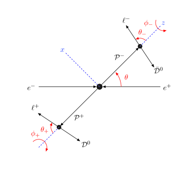
Figure 3: The coordinate system in the colliding $e^{+}e^{-}$ c.m. frame. The $y$-axis is chosen along the $\vec{p}_{-}(e^{-})\times\vec{q}_{-}(\mathcal{P}^{-})$ direction and it is pointing towards the observer. The coordinate systems in the $\mathcal{P}^{-}$ and $\mathcal{P}^{+}$ rest frames are obtained from it by boosts along the $z$-axis. The angles $\theta_{\pm}$ and $\phi_{\pm}$ are the polar and azimuthal angles of the lepton $\ell^{\pm}$ associated with the two-body decay of the $\mathcal{P}^{\pm}$ particles in their respective rest frames.

4 Two-body Decays

The decay amplitudes ${\cal D}_{-}$ and ${\cal D}_{+}$ of the two-body decays, $\mathcal{P}^{-}\to\ell^{-}\mathcal{\bar{D}}^{0}$ and $\mathcal{P}^{+}\to\ell^{+}\mathcal{D}^{0}$, are most simply expressed in the $\mathcal{P}^{-}$ and $\mathcal{P}^{+}$ rest frames, respectively. We define each of these frames by a boost of the $e^{+}e^{-}$ c.m. frame along the $z$-axis as shown in Fig. 3. In the $\mathcal{P}^{\mp}$ rest frame, we parameterize the $\ell^{\mp}$ four-momenta, $p_{1}$ and $p_{3}$, as

$$p_{1}^{\mu}=p^{\mu}_{\ell^{-}} = \frac{M^{2}_{\mathcal{P}}-M^{2}_{\mathcal{D}}}{2M_{\mathcal{P}}}\left(1,\sin\theta_{-}\cos\phi_{-},\sin\theta_{-}\sin\phi_{-},\cos\theta_{-}\right)$$ (4.1)

$$p_{3}^{\mu}=p^{\mu}_{\ell^{+}} = \frac{M^{2}_{\mathcal{P}}-M^{2}_{\mathcal{D}}}{2M_{\mathcal{P}}}\left(1,\sin\theta_{+}\cos\phi_{+},\sin\theta_{+}\sin\phi_{+},-\cos\theta_{+}\right)$$ (4.2)

In this convention of the coordinate systems the angles of the charged lepton are chosen as $(\theta_{-},\phi_{-})$ in the $\mathcal{P}^{-}$ decays and $(\pi-\theta_{+},\phi_{+})$ in the $\mathcal{P}^{+}$ decays.

It is a straightforward exercise to evaluate the helicity amplitudes of the decays $\mathcal{P}^{-}\to\ell^{-}\mathcal{\bar{D}}^{0}$ and $\mathcal{P}^{+}\to\ell^{+}\mathcal{D}^{0}$ with the general couplings listed in Appendix A in the $\mathcal{P}^{\mp}$ rest frames described before. Generically, when the charged lepton masses are ignored, the decay amplitudes can be written as

$${\cal D}_{-}[\mathcal{P}^{-}_{\lambda_{-}}\to\ell^{-}_{\sigma_{1}}\mathcal{\bar{D}}^{0}_{\sigma_{2}}] = e\,K_{\mathcal{PD}}\,D_{-}[\mathcal{P}^{-}\to\ell^{-}\mathcal{\bar{D}}^{0}]_{\sigma_{1}\sigma_{2}}\,d^{J_{\mathcal{P}}}_{\lambda_{-},\sigma_{1}-\sigma_{2}}(\theta_{-})\,{\rm e}^{i(\lambda_{-}-\sigma_{1}+\sigma_{2})\,\phi_{-}}$$ (4.3)

$${\cal D}_{+}[\mathcal{P}^{+}_{\lambda_{+}}\to\ell^{+}_{\sigma_{3}}\mathcal{D}^{0}_{\sigma_{4}}] = e\,K_{\mathcal{PD}}\,D_{+}[\mathcal{P}^{+}\to\ell^{+}\mathcal{D}^{0}]_{\sigma_{3}\sigma_{4}}\,d^{J_{\mathcal{P}}}_{\lambda_{+},\sigma_{3}-\sigma_{4}}(\theta_{+})\,{\rm e}^{-i(\lambda_{+}-\sigma_{3}+\sigma_{4})\,\phi_{+}}$$ (4.4)

with $K_{\mathcal{PD}}=\sqrt{M^{2}_{\mathcal{P}}-M^{2}_{\mathcal{D}}}$ and $\lambda_{-}(\lambda_{+}),\sigma_{1}(\sigma_{3})$ and $\sigma_{2}(\sigma_{4})$ the helicities of the particles $\mathcal{P}^{-}(\mathcal{P}^{+}),\ell^{-}(\ell^{+})$ and $\mathcal{\bar{D}}^{0}(\mathcal{D}^{0})$. We obtain for all the decay combinations with $\mathcal{P}^{\pm}=S^{\pm}_{p},F^{\pm}_{p},V^{\pm}_{p}$ and $\mathcal{D}^{0}=F^{0}_{d},S^{0}_{d},V^{0}_{d}$ the reduced decay helicity amplitudes:

$$D_{-}[S^{-}_{p}\to\ell^{-}\bar{F}^{0}_{d}]_{\sigma_{1}\sigma_{2}} = \delta_{\sigma_{2}\sigma_{1}}\,d^{\ell F}_{S\sigma_{1}}$$ (4.5)

$$D_{-}[F^{-}_{p}\to\ell^{-}\,\bar{S}^{0}_{d}]_{\sigma_{1}}\ \ = d^{\ell S}_{F\sigma_{1}}$$ (4.6)

$$D_{-}[F^{-}_{p}\to\ell^{-}\bar{V}^{0}_{d}]_{\sigma_{1}\sigma_{2}} = -\left[\sqrt{2}\,\delta_{\sigma_{2}\sigma_{1}}+\delta_{\sigma_{2}0}(M_{F_{p}}/M_{V_{d}})\right]d^{\ell V}_{F\sigma_{1}}$$ (4.7)

$$D_{-}[V^{-}_{p}\to\ell^{-}\bar{F}^{0}_{d}]_{\sigma_{1}\sigma_{2}} = \left[\delta_{\sigma_{2}\sigma_{1}}(M_{F_{d}}/M_{V_{p}})+\sqrt{2}\,\delta_{\sigma_{2},-\sigma_{1}}\right]d^{\ell F}_{V\sigma_{1}}$$ (4.8)

and the reduced decay amplitudes for the charge-conjugated decays $\mathcal{P}^{+}\to\ell^{+}\mathcal{D}^{0}$ are given by the relation

$$D_{+}[\mathcal{P}^{+}\to\ell^{+}\mathcal{D}^{0}]_{\sigma_{3}\sigma_{4}}=\mp D_{-}[\mathcal{P}^{-}\to\ell^{-}\mathcal{\bar{D}}^{0}]^{*}_{-\sigma_{3},-\sigma_{4}}$$ (4.9)

up to an overall sign. The sign $+$ is for $\mathcal{P}^{\pm}=V^{\pm}_{p}$ and the sign $-$ for $\mathcal{P}^{\pm}=S^{\pm}_{p},F^{\pm}_{p}$.

5 Full angular-correlations of the final-state leptons

In this section we present the most general angular distribution of the decay products in the correlated production-decay process, following the formalism in Ref. Hagiwara:1986vm

$$e^{-}(p_{-},\sigma_{-})+e^{+}(p_{+},\sigma_{+})\, \to \,\mathcal{P}^{-}(q_{-},\lambda_{-})+\mathcal{P}^{+}(q_{+},\lambda_{+})$$

$$\mathcal{P}^{-}(q_{-},\lambda_{-})\, \to \,\ell^{-}(p_{1},\sigma_{1})+\mathcal{\bar{D}}^{0}(p_{2},\sigma_{2})$$

$$\mathcal{P}^{+}(q_{+},\lambda_{+})\, \to \,\ell^{+}(p_{3},\sigma_{3})+\mathcal{D}^{0}(p_{4},\sigma_{4})$$ (5.1)

with two visible massless charged leptons $\ell^{\pm}$ and two invisible neutral particles $\mathcal{D}^{0}$ and $\mathcal{\bar{D}}^{0}$ in the final state. Combining the production process and two decay processes, we can extract explicitly the dependence of the correlated cross section on final charged lepton angles as well as the production angles and beam polarizations.

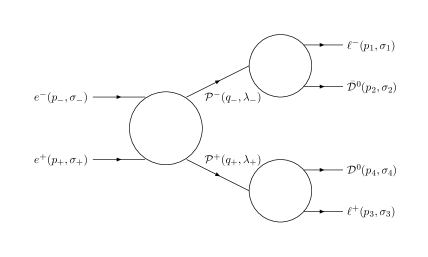
Figure 4: A schematic view of the process $e^{+}e^{-}\,\to\,\mathcal{P}^{+}\mathcal{P}^{-}\,\to\,(\ell^{+}\mathcal{D}^{0})(\ell^{-}\mathcal{\bar{D}}^{0})$. Shown in the parentheses are the four-momenta and re-scaled helicities of the corresponding particles.

5.1 Derivation of the correlated distributions

The fully production-decay correlated amplitudes can be expressed in terms of the production and decay helicity amplitudes as follows:

$${\cal M}(p_{-},\sigma_{-};p_{+},\sigma_{+};p_{1,2},\sigma_{1,2};p_{3,4},\sigma_{3,4}) = \Pi_{\mathcal{P}^{-}}(q^{2}_{-})\,\Pi_{\mathcal{P}^{+}}(q^{2}_{+})\sum_{\lambda_{-},\lambda_{+}}{\cal M}(p_{-},\sigma_{-};p_{+},\sigma_{+};q_{-},\lambda_{-};q_{+},\lambda_{+})$$ (5.2)

$$\times{\cal D}_{-}(q_{-},\lambda_{-};p_{1},\sigma_{1};p_{2},\sigma_{2})\times{\cal D}_{+}(q_{+},\lambda_{+};p_{3},\sigma_{3};p_{4},\sigma_{4})$$

where the Breit-Wigner propagator factors $\Pi_{\mathcal{P}^{\pm}}$ for the $\mathcal{P}^{\pm}$ particles are

$$\Pi_{\mathcal{P}^{\pm}}(q^{2}_{\pm})=(q^{2}_{\pm}-M^{2}_{\mathcal{P}}+iM_{\mathcal{P}}\Gamma_{\mathcal{P}})^{-1}$$ (5.3)

Here we take the summations over intermediate $\mathcal{P}^{\pm}$ polarizations in the helicity basis, i.e. helicities, which are most convenient for theoretical considerations.

In the c.m. frame of the colliding $e^{+}e^{-}$ beams, we choose the $\mathcal{P}^{-}$ momentum direction as the $z$-axis and the $\vec{p}_{-}(e^{-})\times\vec{q}_{-}(\mathcal{P}^{-})$ direction as the $y$-axis so that the scattering $e^{+}e^{-}\to\mathcal{P}^{+}\mathcal{P}^{-}$ takes place in the $x$-$z$ plane (see Fig. 3). The production amplitude ${\cal M}$ is then a function of the scattering angle $\theta$ between $e^{-}$ and $\mathcal{P}^{-}$ momentum directions, as explicitly shown in the previous section. The explicit form of the production amplitude and two decay amplitudes in the $e^{+}e^{-}$ c.m. frame can be derived by the relations:

$${\cal M}(p_{-},\sigma_{-};p_{+},\sigma_{+};q_{-},\lambda_{-};q_{+},\lambda_{+}) = {\cal M}[e^{-}_{\sigma_{-}}e^{+}_{\sigma_{+}}\to\mathcal{P}^{-}_{\lambda_{-}}\mathcal{P}^{+}_{\lambda_{+}}]$$ (5.4)

$${\cal D}_{-}(q_{-},\lambda_{-};p_{1},\sigma_{1};p_{2},\sigma_{2}) = {\cal D}_{-}[\mathcal{P}^{-}_{\lambda_{-}}\to\ell^{-}_{\sigma_{1}}\mathcal{\bar{D}}^{0}_{\sigma_{2}}]$$ (5.5)

$${\cal D}_{+}(q_{+},\lambda_{+};p_{3},\sigma_{3};p_{4},\sigma_{4}) = {\cal D}_{+}[\mathcal{P}^{+}_{\lambda_{+}}\to\ell^{+}_{\sigma_{3}}\mathcal{D}^{0}_{\sigma_{4}}]$$ (5.6)

with the expressions defined in Eq. (3.2) for the production amplitudes and Eqs. (4.3) and (4.4) for the decay amplitudes, respectively.

5.2 Polarization-weighted cross sections

Generally, the full correlations of the production and two two-body decay processes can contain maximally $2^{4}\times(2J_{\mathcal{P}}+1)^{4}$ independent observables expressed in terms of the $e^{+}e^{-}$ c.m. energy $\sqrt{s}$ and six production and decay angles - two angles $(\theta,\varphi)$ for the production process and four angles $(\theta_{\pm},\phi_{\pm})$ for two decay processes - for arbitrarily-polarized electron and positron beams. (Here, $J_{\mathcal{P}}$ is the spin of the particle $\mathcal{P}^{\pm}$.) The factor $2^{4}=16$ comes from the production part and the other $(2J_{\mathcal{P}}+1)^{4}$ ($=1,\,16$ and $81$ for $J_{\mathcal{P}}=0,1/2$ and $1$) from the production-decay correlations.

The polarization-weighted squared matrix elements can be cast into a decomposed form:

$$\overline{\sum}\left|{\cal M}\right|^{2}=\left|\Pi_{\mathcal{P}^{-}}(q^{2}_{-})\right|^{2}\left|\Pi_{\mathcal{P}^{+}}(q^{2}_{+})\right|^{2}\,{\cal P}^{\lambda_{-}\lambda_{+}}_{\lambda^{\prime}_{-}\lambda^{\prime}_{+}}\,{\cal D}^{\lambda_{-}}_{\lambda^{\prime}_{-}}\,\overline{\cal D}^{\lambda_{+}}_{\lambda^{\prime}_{+}}$$ (5.7)

with the summation over repeated indices $(\lambda_{-},\lambda^{\prime}_{-},\lambda_{+},\lambda^{\prime}_{+})$ assumed here and in the following equations. The polarization-weighted production tensor reads

$${\cal P}^{\lambda_{-}\lambda_{+}}_{\lambda^{\prime}_{-}\lambda^{\prime}_{+}}=\sum_{\sigma_{-},\sigma^{\prime}_{-}}\sum_{\sigma_{+},\sigma^{\prime}_{+}}\,P^{-}_{\sigma_{-}\sigma^{\prime}_{-}}P^{+}_{\sigma_{+}\sigma^{\prime}_{+}}\,{\cal M}[e^{-}_{\sigma_{-}}e^{+}_{\sigma_{+}}\to\mathcal{P}^{-}_{\lambda_{-}}\mathcal{P}^{+}_{\lambda_{+}}]\,{\cal M}^{*}[e^{-}_{\sigma_{-}}e^{+}_{\sigma_{+}}\to\mathcal{P}^{-}_{\lambda^{\prime}_{-}}\mathcal{P}^{+}_{\lambda^{\prime}_{+}}]$$ (5.8)

in terms of the production helicity amplitudes, where the electron and positron polarization tensors $P^{\mp}$ are given in the $(+,-)$ helicity basis by Hagiwara:1985yu

$$P^{-}_{\sigma_{-}\sigma^{\prime}_{-}} = \frac{1}{2}\left(\begin{array}[]{cc}1+P^{L}_{-}&P^{T}_{-}{\rm e}^{-i\phi_{-}}\\[5.69054pt] P^{T}_{-}{\rm e}^{i\phi_{-}}&1-P^{L}_{-}\end{array}\right)$$ (5.11)

$$P^{+}_{\sigma_{+}\sigma^{\prime}_{+}} = \frac{1}{2}\left(\begin{array}[]{cc}1+P^{L}_{+}&P^{T}_{+}{\rm e}^{-i\phi_{+}}\\[5.69054pt] P^{T}_{+}{\rm e}^{i\phi_{+}}&1-P^{L}_{+}\end{array}\right)$$ (5.14)

respectively, where $\phi_{-}=-\varphi$ and $\phi_{+}=-\varphi+\delta$ with the azimuthal angle $\varphi$ of the $\mathcal{P}^{-}$ flight direction as measured from the electron transverse polarization direction and $\delta$ the relative opening angle of the electron and positron transverse-polarization directions. Details of this calculation for incorporating beam polarizations are given in Appendix C. The decay density matrices with the daughter particle polarizations summed in Eq. (5.7) are given by

$${\cal D}^{\lambda_{-}}_{\lambda^{\prime}_{-}}(\theta_{-},\phi_{-}) = \sum_{\sigma_{1},\sigma_{2}}{\cal D}_{-}[\mathcal{P}^{-}_{\lambda_{-}}\to\ell^{-}_{\sigma_{1}}\mathcal{\bar{D}}^{0}_{\sigma_{2}}]\,{\cal D}^{*}_{-}[\mathcal{P}^{-}_{\lambda^{\prime}_{-}}\to\ell^{-}_{\sigma_{1}}\mathcal{\bar{D}}^{0}_{\sigma_{2}}]$$ (5.15)

$$\overline{\cal D}^{\lambda_{+}}_{\lambda^{\prime}_{+}}(\theta_{+},\phi_{+}) = \sum_{\sigma_{3},\sigma_{4}}{\cal D}_{+}[\mathcal{P}^{+}_{\lambda_{+}}\to\ell^{+}_{\sigma_{3}}\mathcal{D}^{0}_{\sigma_{4}}]\,{\cal D}^{*}_{+}[\mathcal{P}^{+}_{\lambda^{\prime}_{+}}\to\ell^{+}_{\sigma_{3}}\mathcal{D}^{0}_{\sigma_{4}}]$$ (5.16)

After integration over the virtual $\mathcal{P}$ masses squared, $q^{2}_{-}$ and $q^{2}_{+}$, the unpolarized differential cross section can be expressed in the narrow width approximation as

$$\frac{d\sigma}{d\cos\theta d\varphi\,d\cos\theta_{-}d\phi_{-}d\cos\theta_{+}d\phi_{+}}=\frac{(2J_{\mathcal{P}}+1)^{2}\beta}{1024\pi^{4}s}\,{\rm Br}[\mathcal{P}^{-}\to\ell^{-}\mathcal{\bar{D}}^{0}]\,{\rm Br}[\mathcal{P}^{+}\to\ell^{+}\mathcal{D}^{0}]\,\,{\cal P}^{\lambda_{-}\lambda_{+}}_{\lambda^{\prime}_{-}\lambda^{\prime}_{+}}\,\rho^{\lambda_{-}}_{\lambda^{\prime}_{-}}\,\overline{\rho}^{\lambda_{+}}_{\lambda^{\prime}_{+}}$$ (5.17)

with $\beta=(1-4M^{2}_{\mathcal{P}}/s)^{1/2}$. Here, $\rho$ and $\overline{\rho}$ are the normalized decay density matrices defined as

$$\rho^{\lambda_{-}}_{\lambda^{\prime}_{-}}=\frac{{\cal D}^{\lambda_{-}}_{\lambda^{\prime}_{-}}}{{\rm Tr}({\cal D})}\quad\,\mbox{and}\quad\,\overline{\rho}^{\lambda_{+}}_{\lambda^{\prime}_{+}}=\frac{\overline{\cal D}^{\lambda_{+}}_{\lambda^{\prime}_{+}}}{{\rm Tr}(\overline{\cal D})}$$ (5.18)

satisfying the normalization conditions ${\rm Tr}(\rho)=1$ and ${\rm Tr}(\overline{\rho})=1$. With this normalization condition the overall constant $\mathcal{K}$ is fixed in terms of the branching fractions ${\rm Br}(\mathcal{P}^{-}\to\ell^{-}\mathcal{\bar{D}}^{0})$ and ${\rm Br}(\mathcal{P}^{+}\to\ell^{+}\mathcal{D}^{0})$. By integrating over $\mathcal{P}^{+}$ decays, we obtain the inclusive $\mathcal{P}^{-}\to\ell^{-}\mathcal{\bar{D}}^{0}$ decay distribution

$$\frac{d\sigma}{d\cos\theta d\varphi\,d\cos\theta_{-}d\phi_{-}}=\frac{(2J_{\mathcal{P}}+1)\beta}{256\pi^{3}s}\,{\rm Br}[\mathcal{P}^{-}\to\ell^{-}\mathcal{\bar{D}}^{0}]\,\,{\cal P}^{\lambda_{-}\lambda_{+}}_{\lambda^{\prime}_{-}\lambda_{+}}\,\rho^{\lambda_{-}}_{\lambda^{\prime}_{-}}$$ (5.19)

and alternatively we obtain the $\mathcal{P}^{+}\to\ell^{+}\mathcal{D}^{0}$ decay distribution as

$$\frac{d\sigma}{d\cos\theta d\varphi\,d\cos\theta_{+}d\phi_{+}}=\frac{(2J_{\mathcal{P}}+1)\beta}{256\pi^{3}s}\,{\rm Br}[\mathcal{P}^{+}\to\ell^{+}\mathcal{D}^{0}]\,\,{\cal P}^{\lambda_{-}\lambda_{+}}_{\lambda_{-}\lambda^{\prime}_{+}}\,\overline{\rho}^{\lambda_{+}}_{\lambda^{\prime}_{+}}$$ (5.20)

By further integrating out all the decay lepton angles, we simply get the unpolarized differential cross section for the production process $e^{+}e^{-}\to\mathcal{P}^{+}\mathcal{P}^{-}$:

$$\frac{d\sigma}{d\cos\theta d\varphi}=\frac{\beta}{64\pi^{2}s}\,{\cal P}^{\lambda_{-}\lambda_{+}}_{\lambda_{-}\lambda_{+}}$$ (5.21)

whose explicit form for the process $e^{+}e^{-}\to\mathcal{P}^{+}\mathcal{P}^{-}$ can be found in Eq. (3.3). By comparing Eqs. (5.17), (5.19) and (5.20) with Eq. (5.21) we can get the additional information on not only the $\mathcal{P}^{+}\mathcal{P}^{-}$ production amplitudes but also the $\mathcal{P}^{\pm}$ decay amplitudes encoded in decay lepton angular distributions.

5.3 Decay density matrices

The explicit form of the normalized decay density matrix for each spin combination of the parent and daughter particles, $\mathcal{P}^{-}$ and $\mathcal{\bar{D}}^{0}$, in the decay $\mathcal{P}^{-}\to\ell^{-}\mathcal{\bar{D}}^{0}$ can be derived with the explicit form of each decay amplitude listed in Eqs. (4.5), (4.6), (4.7) and (4.8), respectively. For the spin-0 case with $\mathcal{P}^{-}=S^{-}_{p}$ and $\mathcal{\bar{D}}^{0}=F^{0}_{d}$, the decay matrix is a single number:

$$\rho[S^{-}_{p}\to\ell^{-}\bar{F}^{0}_{d}]=1$$ (5.22)

generating no production-decay correlations, independently of the chiral structure of the couplings. On the other hand, for the two spin-1/2 cases, the $2\times 2$ decay density matrices read

$$\rho[F^{-}_{p}\to\ell^{-}\bar{S}^{0}_{d}]=\frac{1}{2}\left(\begin{array}[]{cc}1+\xi_{\rm fs}\cos\theta_{-}&\xi_{\rm fs}\sin\theta_{-}{\rm e}^{i\phi_{-}}\\ \xi_{\rm fs}\sin\theta_{-}{\rm e}^{-i\phi_{-}}&1-\xi_{\rm fs}\cos\theta_{-}\end{array}\right)\ \ \mbox{with}\ \ \xi_{\rm fs}=\frac{|d^{\ell S}_{F+}|^{2}-|d^{\ell S}_{F-}|^{2}}{|d^{\ell S}_{F+}|^{2}+|d^{\ell S}_{F-}|^{2}}$$ (5.25)

for the spin-0 daughter particle $\bar{S}^{0}_{d}$ and

$$\rho[F^{-}_{p}\to\ell^{-}\bar{V}^{0}_{d}] = \frac{1}{2}\left(\begin{array}[]{cc}1+\xi_{\rm fv}\eta_{\rm fv}\cos\theta_{-}&\xi_{\rm fv}\eta_{\rm fv}\sin\theta_{-}{\rm e}^{i\phi_{-}}\\ \xi_{\rm fv}\eta_{\rm fv}\sin\theta_{-}{\rm e}^{-i\phi_{-}}&1-\xi_{\rm fv}\eta_{\rm fv}\cos\theta_{-}\end{array}\right)$$ (5.29)

$$\mbox{with}\ \ \eta_{\rm fv}=\frac{M^{2}_{F_{p}}-2M^{2}_{V_{d}}}{M^{2}_{F_{p}}+2M^{2}_{V_{d}}}\ \ \mbox{and}\ \ \xi_{\rm fv}=\frac{|d^{\ell V}_{F+}|^{2}-|d^{\ell V}_{F-}|^{2}}{|d^{\ell V}_{F+}|^{2}+|d^{\ell V}_{F-}|^{2}}$$

for the spin-1 daughter particle $\bar{V}^{0}_{d}$, and the $3\times 3$ decay density matrix for the spin-1 parent particle $V^{-}_{p}$ reads:

$$\rho[V^{-}_{p}\to\ell^{-}\bar{F}^{0}_{d}] = (1-\eta_{\rm vf})\,\mathbb{1}_{3\times 3}+(3\eta_{\rm vf}-2)\,\rho_{T}+\xi_{\rm vf}\,\eta_{\rm vf}\,\delta_{T}$$ (5.30)

$$\mbox{with}\ \ \eta_{\rm vf}=\frac{2M^{2}_{V_{p}}}{2M^{2}_{V_{p}}+M^{2}_{F_{d}}}\ \ \mbox{and}\ \ \xi_{\rm vf}=\frac{|d^{\ell F}_{V+}|^{2}-|d^{\ell F}_{V-}|^{2}}{|d^{\ell F}_{V+}|^{2}+|d^{\ell F}_{V-}|^{2}}$$

where $\mathbb{1}_{3\times 3}$ is the $3\times 3$ identity matrix, and the normalized matrix $\rho_{T}$ and the traceless matrix $\delta_{T}$ are given by

$$\rho_{T}=\frac{1}{4}\,\left(\begin{array}[]{ccc}1+c^{2}_{-}&\sqrt{2}c_{-}s_{-}{\rm e}^{i\phi_{-}}&s^{2}_{-}{\rm e}^{2i\phi_{-}}\\ \sqrt{2}c_{-}s_{-}{\rm e}^{-i\phi_{-}}&2s^{2}_{-}&-\sqrt{2}c_{-}s_{-}{\rm e}^{i\phi_{-}}\\ s^{2}_{-}{\rm e}^{-2i\phi_{-}}&-\sqrt{2}c_{-}s_{-}{\rm e}^{-i\phi_{-}}&1+c_{-}^{2}\end{array}\right)$$ (5.34)

$$\delta_{T}=\frac{1}{4}\,\left(\begin{array}[]{ccc}2c_{-}&\sqrt{2}s_{-}{\rm e}^{i\phi_{-}}&0\\ \sqrt{2}s_{-}{\rm e}^{-i\phi_{-}}&0&\sqrt{2}s_{-}{\rm e}^{i\phi_{-}}\\ 0&\sqrt{2}s_{-}{\rm e}^{-i\phi_{-}}&-2c_{-}\end{array}\right)$$ (5.38)

with the abbreviations $c_{-}=\cos\theta_{-}$ and $s_{-}=\sin\theta_{-}$.

The density matrices for the charge-conjugated decays $\mathcal{P}^{+}\to\ell^{+}\mathcal{D}^{0}$ are related to those of the decays $\mathcal{P}^{-}\to\ell^{-}\mathcal{\bar{D}}^{0}$ as follows:

$$\overline{\rho}[\mathcal{P}^{+}\to\ell^{+}\mathcal{D}^{0}]=\rho[\mathcal{P}^{-}\to\ell^{-}\mathcal{\bar{D}}^{0}]\,\left(\theta_{-}\to\theta_{+},\,\phi_{-}\to-\phi_{+},\,\xi\to-\xi\right)$$ (5.39)

The two density matrices can be used for describing non-trivial final-state angular correlations between two visible leptons through the connection linked by the production process.

As shown clearly by the expressions in Eqs. (5.25), (5.29) and (5.30), the decay distributions are affected not just by the spins and masses of the particles but also the chiralities of their couplings. We find:

• If the relative chirality $\xi_{\rm fs}$ is zero, i.e. the coupling is either pure vector-like or pure axial-vector-like, the decay density matrix becomes an identity matrix, washing out any correlation in the final-state leptons of the decays $F^{-}_{p}\to\ell^{-}\bar{S}^{0}_{d}$ and $F^{+}_{p}\to\ell^{+}S^{0}_{d}$ completely. On the contrary, if the coupling is purely chiral with $\xi_{\rm fs}=\pm 1$, the decay distributions provide maximal information on the production-decay correlations.

• In addition to the relative chirality $\xi_{\rm fv}$ there exists a kinematic factor $\eta_{\rm fv}$ determining the polarization analysis power in the decay $F^{-}_{p}\to\ell^{-}\bar{V}^{0}_{d}$. This purely mass-dependent factor vanishes for the special case with $M_{F_{p}}=\sqrt{2}M_{V_{d}}$ and takes its maximum value of unity only when $M_{V_{d}}=0$, i.e. the spin-1 daughter particle $V^{0}_{d}$ is massless. Nevertheless, if the coupling is purely chiral, then this decay mode with a spin-1 daughter particle can be distinguished from the decay mode with a spin-0 daughter particle by measuring the polarization analysis power; in the latter case its magnitude is 1 and in the former case its magnitude is $\eta_{\rm fv}<1$ for $M_{V_{d}}>0$.

• In the spin-1 case, if the relative chirality $\xi_{\rm vf}$ is zero, the density matrix becomes an identity matrix only when the parent and daughter particles are degenerate, i.e. $M_{V_{p}}=M_{F_{d}}$. However, in this degenerate case, the decay is kinematically forbidden. Therefore, we can conclude that the spin-1 case can be distinguished from the spin-0 and spin-1/2 cases.

Before closing this subsection, we emphasize that, with all these spin- and chirality-dependent characteristics of the decay density matrices, the decay angle correlations of the final-state leptons become trivial unless the parent particles are polarized as will be demonstrated below.

6 Observables

In the last section, we gave a detailed description of the angular distribution of the final-state lepton-antilepton pairs arising from the decay of the $\mathcal{P}^{+}\mathcal{P}^{-}$ pair. Schematically, the 6-fold differential cross section has the form

$$d\sigma\ \ \sim\ \ \sum^{N_{\rm tot}}\,\mathrm{P}_{i}(P^{L}_{-},P^{L}_{+};P^{T}_{-},P^{T}_{+},\delta;\theta,\varphi;\sqrt{s})\,\,\mathrm{D}_{i}(\theta_{-},\phi_{-},\theta_{+},\phi_{+})\quad\mbox{with}\quad N_{\rm tot}=(2J_{\mathcal{P}}+1)^{4}$$ (6.1)

Here the functions $\mathrm{D}_{i}$ form a linearly independent set consisting of low-energy spherical harmonics, which reflects the decay dynamics. The dynamics of the production process is solely contained in the factors $\mathrm{P}_{i}$, forming maximally 16 independent terms. These are given essentially by the density matrix of the $\mathcal{P}^{+}\mathcal{P}^{-}$ pair and by beam polarizations. The fact that we can in principle measure $16\times(2J_{\mathcal{P}}+1)^{4}$ functions shows that it is possible to extract an enormous amount of information on the production and decay mechanism.

However, unless we have a sufficient number of events, it is neither possible nor practical to perform a fit with the large number of all independent angular and/or polarization distributions. Rather it is meaningful to obtain from the experimental data a specific set of observables depending on the c.m. energy, the beam polarizations, the production angles and the decay angular distributions that are efficiently controllable and reconstructible and sensitive to the spin and chirality effects. In the following numerical analysis we restrict ourselves to five conventional kinematic variables — the beam energy $\sqrt{s}$, the production polar angle $\theta$, the two lepton polar angles, $\theta_{-}$ and $\theta_{+}$, in the decays, $\mathcal{P}^{-}\to\ell^{-}\mathcal{\bar{D}}^{0}$ and $\mathcal{P}^{+}\to\ell^{+}\mathcal{D}^{0}$, and the cosine of the azimuthal-angle difference $\phi$ between two decay planes. The impact of beam polarizations on each observable is also diagnosed numerically.

In order to gauge the sensitivities of the observables mentioned in the previous subsection to spin and chirality effects in the antler-topology processes, we investigate their distributions for ten typical spin and chirality assignments as shown with five examples from the MSSM and five examples from the MUED listed in Tab. 3. For the sake of simplicity, when describing the specific examples, we impose electron chirality invariance (which is valid to a very good precision in the popular models MSSM and MUED), forcing us to neglect any $s$-channel scalar contributions and to set any three-point $e\mathcal{T}\mathcal{P}$ and $\mathcal{P}\ell\mathcal{D}$ vertices with $\ell=e,\mu$ to be purely chiral in the $t$-channel diagram and the two-body decay diagrams. Furthermore, in the present numerical analysis we do not have any $u$-channel exchange of doubly-charged particles, for which new higher representations of the SM gauge group have to be introduced in the theories. In any case, note that in principle all the $u$-channel contributions, if they exist, can be worked out through the analytic expressions presented in Sect. 3. For example, the major difference between a $u$-channel process and a $t$-channel process is that the production polar-angle distribution will be backward-peaked instead of forward-peaked, as can be seen from Eq. (3.18).

Index	$[J_{\mathcal{P}},J_{\mathcal{D}}]$	Chirality	Antler-topology process	$s$-channel $[J_{\mathcal{S}^{0}}]$	$t$-channel $[J_{\mathcal{T}^{0}}]$	Model
$A_{L/R}$	$[0,1/2]$	$L/R$	$e^{+}e^{-}\to\tilde{\mu}^{+}_{L/R}\tilde{\mu}^{-}_{L/R}\to(\mu^{+}\tilde{B})(\mu^{-}\tilde{B})$	$\gamma,Z$   $[J=1]$	$-$	MSSM
$B_{L/R}$	$[0,1/2]$	$L/R$	$e^{+}e^{-}\to\tilde{e}^{+}_{L/R}\tilde{e}^{-}_{L/R}\to(e^{+}\tilde{B})(e^{-}\tilde{B})$	$\gamma,Z$   $[J=1]$	$\tilde{B},\tilde{W}^{0}$  $[J=1/2]$	MSSM
$C_{L/R}$	$[1/2,1]$	$L/R$	$e^{+}e^{-}\to\mu^{+}_{L1/R1}\mu^{-}_{L1/R1}\to(\mu^{+}B_{1})(\mu^{-}B_{1})$	$\gamma,Z$   $[J=1]$	$-$	MUED
$D_{L/R}$	$[1/2,1]$	$L/R$	$e^{+}e^{-}\to e^{+}_{L1/R1}e^{-}_{L1/R1}\to(e^{+}B_{1})(e^{-}B_{1})$	$\gamma,Z$   $[J=1]$	$B_{1},W^{0}_{1}$   $[J=1]$	MUED
$E_{L}$	$[1/2,0]$	$L$	$e^{+}e^{-}\to\tilde{W}^{+}\tilde{W}^{-}\to(\ell^{+}\tilde{\nu}_{\ell})(\ell^{-}\tilde{\nu}^{*}_{\ell})$	$\gamma,Z$   $[J=1]$	$\tilde{\nu}_{e}$  $[J=0]$	MSSM
$F_{L}$	$[1,1/2]$	$L$	$e^{+}e^{-}\to W^{+}_{1}W^{-}_{1}\to(\ell^{+}\nu_{\ell 1})(\ell^{-}\bar{\nu}_{\ell 1})$	$\gamma,Z$   $[J=1]$	$\nu_{e1}$   $[J=1/2]$	MUED

Table 3: Ten examples for the antler-topology processes - five in MSSM and five in MUED. Every ECV effect due to EWSB in these models is small so that the $e\mathcal{T}\mathcal{P}$ and $\mathcal{P}\ell\mathcal{D}$ couplings are purely chiral to very good approximation. The first index is introduced to specify each spin and chirality assignment. The chirality index, $R$ or $L$, in the third column stands for the chiral structure of the $e^{-}\mathcal{T}^{0}\mathcal{P}^{-}$ vertex and the $\mathcal{P}^{-}\ell^{-}\mathcal{\bar{D}}^{0}$ vertex. We note that the chirality of each $t$-channel coupling is identical to the chirality of the vertex describing the decay $\mathcal{P}^{-}\to\ell^{-}\mathcal{\bar{D}}^{0}$ in every scenario.

In general several particles may contribute to the $s$-channel and/or $t$-channel diagrams and the mass spectrum of the new particles depends strongly on the mass generation mechanism unique to each model beyond the SM. Nevertheless, expecting no significant loss of generality, we assume in our numerical analysis that only the SM neutral electroweak gauge bosons $\gamma$ and $Z$ contribute to the $s$-channel diagram and only one or two particles, named $\mathcal{T}^{0}_{1}$ and $\mathcal{T}^{0}_{2}$ when two particles are involved, are exchanged in the $t$-channel diagram. Then, we take the following simplified mass spectrum:

$$M_{\mathcal{P}}=M_{\mathcal{T}_{2}}=200\,{\rm GeV}\quad\mbox{and}\quad M_{\mathcal{D}}=M_{\mathcal{T}_{1}}=100\,{\rm GeV}$$ (6.2)

We emphasize that the mass spectrum (6.2) is chosen only as a simple illustrative example in the MSSM and MUED models with different spins but similar final states and so the procedure for spin determination demonstrated in the present work can be explored for any other BSM models as well as within the SM itself. The coupling of the $Z$ boson as well as the photon $\gamma$ to the new spin-1/2 charged fermion pair $F^{+}_{p}F^{-}_{p}$ with $\mathcal{P}^{\pm}=F^{\pm}_{p}$ is taken to be purely vector-like, as this is valid for the first Kaluza-Klein (KK) lepton states in MUED with $F^{\pm}_{p}=\ell^{\pm}_{L1/R1}$ and for the pure charged wino or higgsino states in the MSSM with $F^{\pm}_{p}=\tilde{W}^{\pm},\tilde{H}$, valid to very good approximation when the mixing between the gaugino and higgsino states due to EWSB is ignored in the MSSM. It is also assumed that the lightest neutralino is a pure bino, $\tilde{B}$, and the second lightest neutralino is a pure wino, $\tilde{W}^{0}$. In this case, the lightest chargino is almost degenerate with the second lightest neutralino.

Applying all the assumptions mentioned above to the MSSM and MUED processes listed in Tab. 3, we can obtain the full list of non-zero ECC couplings for the processes Chung:2003fi ; Datta:2010us : for the $s$-channel couplings

$$s^{\gamma}_{ee\pm}=s^{\tilde{\ell}_{R}\tilde{\ell}_{R}}_{\gamma}=s^{\tilde{\ell}_{L}\tilde{\ell}_{L}}_{\gamma}=s^{\ell_{R1}\ell_{R1}}_{\gamma\pm}=s^{\ell_{L1}\ell_{L1}}_{\gamma\pm}=s^{\tilde{W}\tilde{W}}_{\gamma\pm}=s^{W_{1}W_{1}}_{\gamma}=1$$ (6.3)

$$s^{Z}_{ee+}=s^{\tilde{\ell}_{R}\tilde{\ell}_{R}}_{Z}=s^{\ell_{R1}\ell_{R1}}_{Z\pm}=-s_{W}/c_{W}$$ (6.4)

$$s^{Z}_{ee-}=s^{\tilde{\ell}_{L}\tilde{\ell}_{L}}_{Z}=s^{\ell_{L1}\ell_{L1}}_{Z\pm}=(1/2-s^{2}_{W})/c_{W}s_{W}$$ (6.5)

$$s^{\tilde{W}\tilde{W}}_{Z\pm}=s^{W_{1}W_{1}}_{Z}=c_{W}/s_{W}$$ (6.6)

with $\ell^{\pm}=e^{\pm},\mu^{\pm}$ and for the $t$-channel and decay couplings

$$t^{e\tilde{e}_{R}}_{\tilde{B}+}=d^{\ell\tilde{B}}_{\tilde{\ell}_{R}-}=-\sqrt{2}/c_{W};\quad t^{e\tilde{e}_{L}}_{\tilde{B}-}=d^{\ell\tilde{B}}_{\tilde{\ell}_{L}+}=1/\sqrt{2}c_{W};\quad t^{e\tilde{e}_{L}}_{\tilde{W}-}=1/\sqrt{2}s_{W},\quad t^{e\tilde{W}}_{\tilde{\nu}_{e}-}=d^{\ell\tilde{\nu}_{\ell}}_{\tilde{W}+}=-1/s_{W}$$ (6.7)

$$t^{ee_{R1}}_{B_{1}+}=d^{\ell B_{1}}_{\ell_{R1}+}=1/c_{W};\quad t^{ee_{L1}}_{B_{1}-}=d^{\ell B_{1}}_{\ell_{L1}-}=1/2c_{W};\quad t^{ee_{L1}}_{W_{1}-}=1/2s_{W};\quad t^{eW_{1}}_{\nu_{e1}-}=d^{\ell\nu_{\ell 1}}_{W_{1}-}=-1/\sqrt{2}s_{W}$$ (6.8)

in the MSSM and in the MUED, respectively. All the other couplings are vanishing in the ECC limit.

6.1 Kinematics

Before presenting the detailed analytic and numerical analysis of spin and chirality effects on each observable, we first describe how each kinematic observable can be constructed for the antler-topology processes. The measurement of the cross section for $\mathcal{P}^{+}\mathcal{P}^{-}$ pair production can be carried out by identifying acoplanar $\ell^{+}\ell^{-}$ pairs with respect to the $e^{\pm}$ beam axis accompanied by large missing energy carried by the invisible $\mathcal{D}^{0}\mathcal{\bar{D}}^{0}$ pairs.

For very high energy $\sqrt{s}\gg M_{\mathcal{P}}$ the flight direction of the parent particle can be approximated by the flight direction of the daughter particles $\ell^{\pm}$ and the dilution due to the decay kinematics is small. However, at medium $e^{+}e^{-}$ energies the dilution increases, and the reconstruction of the $\mathcal{P}^{\pm}$ flight direction provides more accurate results on the angular distribution of the $\mathcal{P}^{\pm}$ pairs. If all particle masses are known, the magnitude of the particle momenta is calculable and the relative orientation of the momentum vectors of $\ell^{\pm}$ and $\mathcal{P}^{\pm}$ is fixed by the two-body decay kinematics:

$$M^{2}_{\mathcal{P}}-M^{2}_{\mathcal{D}}=\sqrt{s}E_{\ell^{\pm}}\left(1-\beta\,\hat{n}_{\mathcal{P}^{\pm}}\cdot\hat{n}_{\pm}\right)=\sqrt{s}\,E_{\ell^{\pm}}\left(1-\beta\cos\alpha_{\pm}\right)$$ (6.9)

where the unit vector $\hat{n}_{\mathcal{P}^{\pm}}$ stands for the $\mathcal{P}^{\pm}$ momentum direction, the unit vectors $\hat{n}_{\pm}$ for the $\ell^{\pm}$ flight directions and the angles $\alpha_{\pm}$ for the opening angles between the visible $\ell^{\pm}$ tracks and the parent $\mathcal{P}^{\pm}$ momentum directions in the $e^{+}e^{-}$ c.m frame. The angles $\alpha_{\pm}$ can be reconstructed event by event by measuring the lepton energies in the laboratory frame, i.e. the $e^{+}e^{-}$ c.m. frame and they define two cones about the $\ell^{+}$ and $\ell^{-}$ axes intersecting in two lines — the true $\mathcal{P}^{\pm}$ flight direction and a false direction. Thus the $\mathcal{P}^{\pm}$ flight direction can be reconstructed up to a two-fold discrete ambiguity.

In contrast to the production angle, the decay polar angles $\theta_{\pm}$ in the $\mathcal{P}^{\pm}$ rest frames can be unambiguously determined event by event independently of the reconstruction of the $\mathcal{P}^{\pm}$ direction by the relation:

$$\cos\theta_{\pm}=\frac{1}{\beta}\left(\frac{E_{\ell^{\pm}}}{E^{*}_{\ell^{\pm}}}-1\right)\quad\mbox{with}\quad E^{*}_{\ell^{\pm}}=\frac{M^{2}_{\mathcal{P}}-M^{2}_{\mathcal{D}}}{2M_{\mathcal{P}}}$$ (6.10)

where $E^{*}_{\ell^{\pm}}$ is the fixed $\ell^{\pm}$ energy in the $\mathcal{P}^{\pm}$ rest frame. Therefore, any decay polar-angle correlations between two leptons in the correlated process can be reconstructed event by event by measuring the lepton energies in the laboratory frame.

Another angular variable, which is reconstructible event by event in the antler-topology processes, is the cosine of the difference $\phi=\phi_{+}-\phi_{-}$ of the azimuthal angles of two leptons with respect to the production plane. Explicitly, it is related to the opening angle of two visible leptons and two polar angles $\alpha_{\pm}$ in the laboratory frame as

$$\cos\phi=\cos(\phi_{+}-\phi_{-})=\frac{\hat{n}_{+}\cdot\hat{n}_{-}+\cos\alpha_{+}\cos\alpha_{-}}{\sin\alpha_{+}\sin\alpha_{-}}$$ (6.11)

Note that the $\cos 2\phi$ distribution also can be measured unambiguously as $\cos 2\phi=2\cos^{2}\phi-1$. In contrast, the sign of the sine of the angular difference of two azimuthal angles is not uniquely determined because of the intrinsic two-fold discrete ambiguity in the determination of the $\mathcal{P}^{\pm}$ flight direction, although its magnitude is determined. (For details, see Appendix D.)

There exist many other types of angular distributions which provide us with additional information on the spin and chirality effects. Nevertheless, while postponing the complete analysis based on the full set of energy and angular distributions, we will study the four kinematic observables $\{\sqrt{s},\,\theta,\,\theta_{-},\,\cos\phi\}$ supplemented with beam polarizations.

6.2 Beam energy dependence and threshold excitation pattern

As described through a detailed analytical investigation before, the excitation curve of the production cross section near threshold in the ECC scenario exhibits its characteristic pattern according to the spin of the produced particle $\mathcal{P}^{\pm}$ and the chiral patterns of the couplings among the on-shell particles and any intermediate particles exchanged in the $s$-, $t$- and/or $u$-channel diagrams.

The production cross section of a spin-0 scalar pair as in the scenario $A_{L/R}$ of the $L$- or $R$-smuon pair production and the scenario $B_{L/R}$ of the $L$- or $R$-selectron pair production shows a characteristic slow $P$-wave threshold excitation, i.e. $\sigma\sim\beta^{3}$, despite the $t$-channel neutral bino and/or wino contributions to the selectron pair production. In contrast, the production cross section of a spin-1/2 fermion pair as in the scenarios $C_{L/R}$ and $D_{L/R}$ for the $L$- or $R$-handed first KK-muon and KK-electron pair production and as in the scenario $E_{L}$ of a wino pair production always exhibits a sharp $S$-wave threshold excitation, i.e. $\sigma\sim\beta$, (due to the unavoidable pure-vector coupling of a photon to the $e^{+}e^{-}$ and $F^{+}_{p}F^{-}_{p}$). The excitation pattern in the scenario $F_{L}$ for the first KK $W$-boson pair production is characterized dominantly by the presence of the $t$-channel contributions, which should be present for preventing the cross section from developing a bad high energy behavior as the $s$-channel $\gamma$ and $Z$ contributions cannot cancel each other at high energies simultaneously for left- and right-chiral couplings. Note that the polarized cross section with perfect right-handed electron polarization does not have the $t$-channel spin-1/2 $\nu_{e1}$ contribution but only the $s$-channel $\gamma$ and $Z$ contributions leading to complete asymptotic cancellation. In this case, the cross section exhibits a slow $P$-wave behavior as in the scalar case. Otherwise, the cross section contains the non-zero $t$-channel $\nu_{e1}$ contribution with the $J_{0}=2$ amplitude finite at threshold so that the cross section rises in a sharp $S$-wave near threshold. These threshold patterns are summarized in Tab. 4.

Spin $J_{\mathcal{P}}$	Polarized cross section	Threshold excitation	Model
$0$	$\sigma_{L/R}[e^{+}e^{-}\to\tilde{\ell}^{+}_{R}\tilde{\ell}^{-}_{R}]$	$\beta^{3}$	MSSM
	$\sigma_{L/R}[e^{+}e^{-}\to\tilde{\ell}^{+}_{L}\tilde{\ell}^{-}_{L}]$	$\beta^{3}$	MSSM
	$\sigma_{L/R}[e^{+}e^{-}\to\ell^{+}_{R1}\ell^{-}_{R1}]$	$\beta$	MUED
$1/2$	$\sigma_{L/R}[e^{+}e^{-}\to\ell^{+}_{L1}\ell^{-}_{L1}]$	$\beta$	MUED
	$\sigma_{L/R}[e^{+}e^{-}\to\tilde{W}^{+}\tilde{W}^{-}]$	$\beta$	MSSM
$1$	$\sigma_{L}[e^{+}e^{-}\to W^{+}_{1}W^{-}_{1}]$	$\beta$	MUED
	$\sigma_{R}[e^{+}e^{-}\to W^{+}_{1}W^{-}_{1}]$	$\beta^{3}$	MUED

Table 4: Threshold excitation of the polarization-weighted total cross sections for the ten MSSM and MUED processes with $\ell=e,\mu$. $\beta=(1-4M^{2}_{\mathcal{P}}/s)^{1/2}$ is the speed of the particle $\mathcal{P}$ in the $e^{+}e^{-}$ c.m. frame. $\sigma_{L/R}$ stands for the polarization-weighted cross section with perfect left-handed or right-handed electron beam polarization.

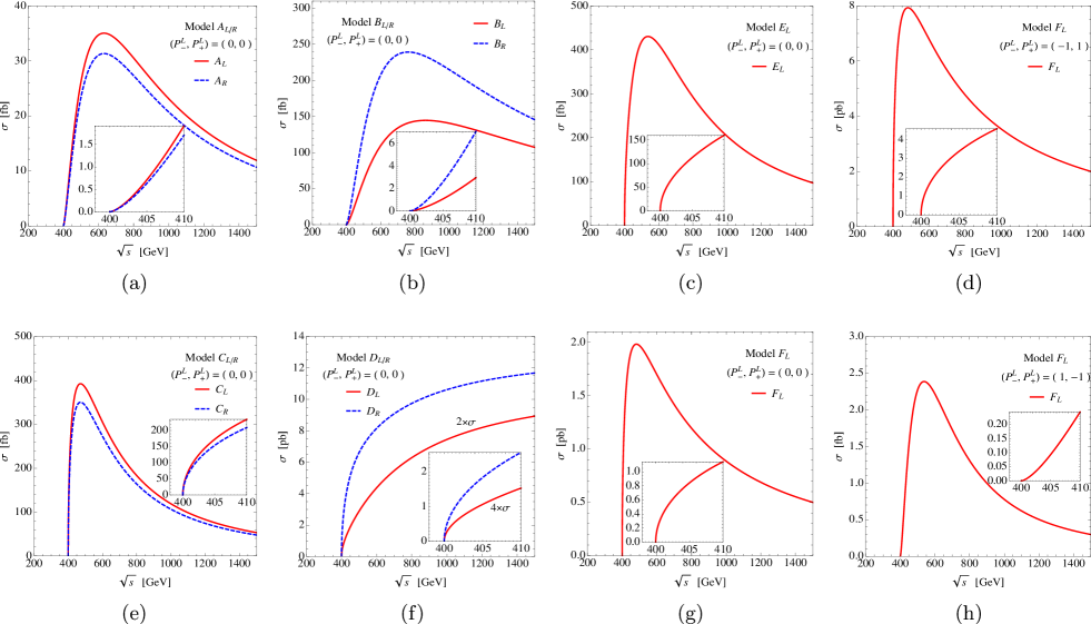
Figure 5: Energy dependence of the total cross sections with the threshold excitation curves embedded for spin-0 scalar bosons ($A_{L/R}$ and $B_{L/R}$), spin-1/2 fermions ($C_{L/R},D_{L/R}$ and $E_{L}$) and spin-1 vector bosons ($F_{L}$). The electron and positron beams are set to be unpolarized, except for the frames, (d) and (h); the upper (lower) frame is for purely left (right) polarized electron and purely right (left) polarized positron beams.

Based on the mass spectrum in Eq. (6.2) and the explicit form of the couplings listed in Eqs. (6.3), (6.4), (6.5), and (6.6) and Eqs. (6.7) and (6.8), we show in Figs. 5 the energy dependence of total cross sections, with the threshold excitation curves embedded, for spin-0 scalar bosons indexed with $A_{L/R}$ and $B_{L/R}$, for spin-1/2 fermions indexed with $C_{L/R}$, $D_{L/R}$ and $E_{L}$, and for spin-1 vector bosons indexed with $F_{L}$. Here, the electron and positron beams are assumed to be unpolarized, except for Figs. 5(d) and (h). In contrast to Figs. 5(d), the plot in Figs. 5(h) clearly shows that the cross section with purely right-handed electron and purely left-handed positron beams killing the $t$-channel contributions while keeping only the $s$-channel spin-1 vector-boson contributions exhibits a slow $P$-wave rise in the excitation curve. We note in passing that it will be crucial to control beam polarization to very good precision in extracting out the right-handed part as the right-handed cross section is more than one thousand times smaller than the left-handed cross section.

To summarize. The threshold energy scan of the polarized cross sections of the pair production process $e^{+}e^{-}\to\mathcal{P}^{+}\mathcal{P}^{-}$ can be very powerful in identifying the spin of the new charged particles $\mathcal{P}^{\pm}$. However, we note that this method may not be fully powerful enough for encompassing the most general scenario including the case with simultaneous left-/right-chiral $t$- and/or $u$-channel contributions and the case with neither of them.

6.3 Polar-angle distribution in the production process

As pointed out before and described in detail in Appendix D, there exists a twofold discrete ambiguity in constructing the production polar angle $\theta$. For very high energy $\sqrt{s}\gg M_{\mathcal{P}}$ the flight direction of the parent particle $\mathcal{P}^{\pm}$ can be approximated by the flight direction of daughter particle $\ell^{\pm}$ and the dilution due to the decay kinematics is small. However, at medium energies the dilution increases and so the reconstruction of the $\mathcal{P}^{\pm}$ flight direction provides more accurate results on the angular distribution of the $\mathcal{P}^{\pm}$ pairs.

Analytically, the angle $\theta_{\rm ft}$ between the false and the true axis is related to the azimuthal angle $\phi$ between two decay planes and to the boosts $\gamma_{\pm}=\gamma(\cos\theta_{\pm}+\beta)$ of the leptons $\ell^{\pm}$ in the laboratory frame as

$$\cos\theta_{\rm ft}=1-\frac{2\sin^{2}\phi}{\gamma^{2}_{+}+\gamma^{2}_{-}+2\gamma_{+}\gamma_{-}\cos\phi+\sin^{2}\phi}$$ (6.12)

For high energies the maximum opening angle reduces effectively to $\theta_{\rm ft}\leq O(1/\gamma)$ and approaches zero asymptotically when the two axes coincide. Quite generally, as a result of the Jacobian root singularity in the relation between $\cos\theta_{\rm ft}$ and $\phi$, the false solutions tend to accumulate slightly near the true axis for all energies Choi:2006mr .

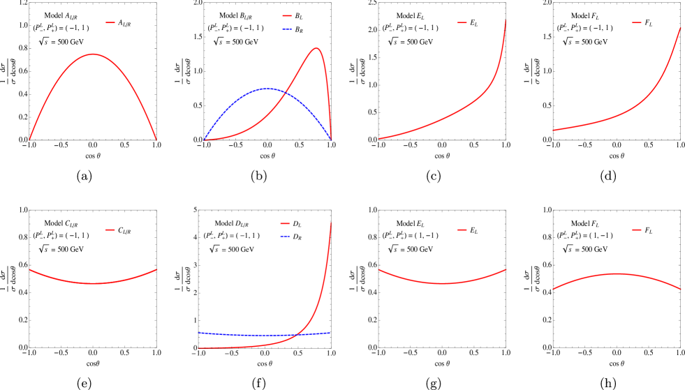
Figure 6: Production polar-angle distributions for the spin-0 scalar bosons indexed with $A_{L/R}$ and $B_{L/R}$, for the spin-1/2 fermions indexed with $C_{L/R},\,D_{L/R}$ and $E_{L}$, and for the spin-1 vector bosons indexed with $F_{L}$ in the MSSM and MUED models. The c.m. energy $\sqrt{s}$ is set to be 500 GeV.

Experimentally, the absolute orientation in space is operationally obtained by rotating the two $\mathcal{P}^{\pm}$ vectors around the $\ell^{\pm}$ axes against each other until they are aligned back to back in opposite directions. The flattened false-axis distribution can be extracted on the basis of Monte Carlo simulations. Figs. 6 shows the normalized production polar-angle distributions for the polarization-weighted differential cross sections, $(1/\sigma_{L/R})\,d\sigma_{L/R}/d\cos\theta$, of the ten processes listed in Tab. 3. The plots in Figs. 6(a) and (b) are for the scalar-pair production processes, $A_{L/R}$ for smuon pairs and $B_{L/R}$ for selectron pairs and the plots in Figs. 6(c), (e), (f) and (g) are for the five fermion-pair production processes, $E_{L}$ for a wino pair, $C_{L/R}$ for the first KK-muon pairs and $D_{L/R}$ for the first KK-electron pairs, respectively, while the two plots in Figs. 6(d) and (h) are for a vector-boson-pair production process, $F_{L}$, for the first KK-$W$ pair.

• From Figs. 6(a) and (b), we find that the cross sections vanish in the forward and back directions with $\cos\theta=\pm 1$ due to the overall angular factor proportional to $\sin^{2}\theta$, independently of the presence of $t$-channel contributions. If the $t$-channel fermion contributions are absent ($A_{L/R}$) or killed by beam polarization ($B_{R}$), the polar-angle distribution is forward and backward symmetric and simply $\sim\sin^{2}\theta$.

• In contrast, the polar-angle distributions for spin-1/2 particles exhibit very distinct angular patterns. If the $t$-channel contributions are absent, as shown in Figs. 6(c), or killed by right-handed electron and left-handed positron beam polarizations, as in Figs. 6(g), the differential cross sections having only the $s$-channel vector-boson contributions with pure vector-type couplings in the three cases have a typical angular distribution $1+\kappa_{1/2}\cos^{2}\theta$ with $\kappa_{1/2}=\beta^{2}/(2-\beta^{2})=0$ at threshold and 1 at asymptotic high energies, leading to the characteristic distribution $1+\cos^{2}\theta$, reflecting the equal contributions of the dominant $(\lambda_{-},\lambda_{+})=(\pm,\mp)$ amplitudes. Once the $t$-channel contributions are included, the angular distribution is severely distorted. Nevertheless, as shown in Figs. 6(c) and (f), the cross sections are peaked at the forward direction.

• Figs. 6(d) and (h) show the angular distributions for spin-1 first KK $W$-boson pair production ($F_{L}$). If the $t$-channel contribution is absent as in Figs. 6(h), the differential cross section has only $s$-channel spin-1 vector-boson contributions with pure vector-type couplings ($F_{L}$) so that the $(\pm\mp)$ amplitudes with $J_{0}=2$ are zero and the $(0,0)$ amplitudes become dominant. As a result, the polar-angle distributions exhibit a characteristic energy-independent polar-angle distribution $\sim 1-\kappa_{1}\cos^{2}\theta$ with the energy-dependent coefficient $\kappa_{1}=3/19$ at threshold and 1 at asymptotically high energies, leading to the simple $\sin^{2}\theta$ distribution identical to the spin-0 case. This asymptotic behavior is a consequence of the so-called Goldstone boson equivalence theorem Cornwall:1974km .

To summarize. The characteristic patterns of the polarized ECC polar-angle distributions can be powerful in determining the spin of $\mathcal{P}^{\pm}$. Evidently it is crucial to have the (longitudinal) polarization of electron and positron beams for the spin determination through the angular distribution. However, we note that the polar-angle distributions alone may not be powerful enough for covering the more general scenarios.

6.4 Single lepton polar-angle distributions in the decays

If the parent particle $\mathcal{P}^{\pm}$ is a spin-0 scalar boson $S^{\pm}_{p}$, there is no production-decay angular correlation at all so that the (normalized) lepton polar-angle distribution is flat, independently of any chirality assignments to the couplings for the production and decay processes as well as of any initial beam polarizations, i.e.

$$\frac{d\sigma^{S}\left[S^{-}_{p}\to\ell^{-}\bar{F}^{0}_{d}\right]}{d\cos\theta d\cos\theta_{-}}=\frac{d\sigma^{S}}{d\cos\theta}\cdot\frac{1}{2}\ \ \Rightarrow\ \ \frac{1}{{\cal C}_{\rm sf}}\frac{d{\cal C}_{\rm sf}}{d\cos\theta_{-}}=\frac{1}{2}$$ (6.13)

The linear relation in Eq. (6.10) between the polar angle $\theta_{\pm}$ and the $\ell^{-}$ energy $E_{\ell^{\pm}}$ indicates that the lepton energy distribution is flat with the energy between $E_{\rm min}=E^{*}_{\ell^{\pm}}(1-\beta)$ and $E_{\rm max}=E^{*}_{\ell^{\pm}}(1+\beta)$ with $\beta=\sqrt{1-4M^{2}_{\mathcal{P}}/s}$.

When the parent particle $\mathcal{P}^{\pm}$ is a spin-1/2 fermion $F^{\pm}_{p}$, then we can directly determine the differential or total cross section for fixed $F_{p}^{\pm}$ helicities by measuring the polar angle distribution of the $F^{\pm}_{p}$ decay products. Depending on the spin of the invisible particle $\mathcal{D}^{0}=S^{0}_{d},V^{0}_{d}$ and the chirality assignments to the $F_{p}S_{d}\ell$ and $F_{p}V_{d}\ell$ couplings, the normalized and correlated polar-angle distributions can be expressed as

$$\frac{d\sigma^{F}[F^{-}_{p}\to\ell^{-}\bar{S}^{0}_{d}]}{d\cos\theta\,d\cos\theta_{-}} = \frac{d\sigma^{F}}{d\cos\theta}\,\cdot\frac{1}{2}\left[1+\xi_{\rm fs}\,\mathbb{P}_{F}\,\cos\theta_{-}\right]\hskip 14.22636pt\ \ \Rightarrow\ \ \frac{1}{{\cal C}_{\rm fs}}\frac{d{\cal C}_{\rm fs}}{d\cos\theta_{-}}=\frac{1}{2}\left[1+\xi_{\rm fs}\,\langle\mathbb{P}_{F}\rangle\,\cos\theta_{-}\right]$$ (6.14)

$$\frac{d\sigma^{F}[F^{-}_{p}\to\ell^{-}\bar{V}^{0}_{d}]}{d\cos\theta\,d\cos\theta_{-}} = \frac{d\sigma}{d\cos\theta}\,\cdot\frac{1}{2}\left[1+\xi_{\rm fv}\eta_{\rm fv}\,\mathbb{P}_{F}\,\cos\theta_{-}\right]\ \ \Rightarrow\ \ \frac{1}{{\cal C}_{\rm fv}}\frac{d{\cal C}_{\rm fv}}{d\cos\theta_{-}}=\frac{1}{2}\left[1+\xi_{\rm fv}\eta_{\rm fv}\,\langle\mathbb{P}_{F}\rangle\,\cos\theta_{-}\right]$$ (6.15)

where two relative chiralities $\xi_{\rm fs}$ and $\xi_{\rm fv}$ and one dilution factor $\eta_{\rm fv}$ are defined by

$$\xi_{\rm fs} = \frac{|d^{\ell S}_{F+}|^{2}-|d^{\ell S}_{F-}|^{2}}{|d^{\ell S}_{F+}|^{2}+|d^{\ell S}_{F-}|^{2}}$$ (6.16)

$$\xi_{\rm fv} = \frac{|d^{\ell V}_{F+}|^{2}-|d^{\ell V}_{F-}|^{2}}{|d^{\ell V}_{F+}|^{2}+|d^{\ell V}_{F-}|^{2}}$$ (6.17)

$$\eta_{\rm fv} = \frac{M^{2}_{F_{p}}-2M^{2}_{V_{d}}}{M^{2}_{F_{p}}+2M^{2}_{V_{d}}}$$ (6.18)

in terms of the chiral coupling coefficients (which are introduced in Appendix A) and the masses $M_{F_{p}}$ and $M_{V_{d}}$, and the differential cross section and the polar-angle dependent polarization observable are defined by

$$\frac{d\sigma^{F}}{d\cos\theta} = \frac{d\sigma^{F}(\lambda_{-}=+)}{d\cos\theta}+\frac{d\sigma^{F}(\lambda_{-}=-)}{d\cos\theta}$$ (6.19)

$$\mathbb{P}_{F} = \left[\frac{d\sigma^{F}(\lambda_{-}=+)}{d\cos\theta}-\frac{d\sigma^{F}(\lambda_{-}=-)}{d\cos\theta}\right]\bigg{/}\frac{d\sigma^{F}}{d\cos\theta}$$ (6.20)

respectively. The average of the polarization observable over the production angle $\theta$ are given by

$$\langle\mathbb{P}_{F}\rangle=\frac{1}{\sigma^{F}}\,\int^{1}_{-1}\mathbb{P}_{F}\,\frac{d\sigma^{F}}{d\cos\theta}\,d\cos\theta=\left(\mathbb{p}^{++}_{++}+\mathbb{p}^{+-}_{+-}\right)-\left(\mathbb{p}^{-+}_{-+}+\mathbb{p}^{--}_{--}\right)$$ (6.21)

satisfying the inequality condition $|\langle\mathbb{P}_{F}\rangle|\leq 1$ in terms of the normalized production tensor $\mathbb{p}$ defined as an integral over the production polar and azimuthal angles $\theta$ and $\varphi$ as

$$\mathbb{p}^{\lambda_{-}\lambda_{+}}_{\lambda^{\prime}_{-}\lambda^{\prime}_{+}}=\int{\cal P}^{\lambda_{-}\lambda_{+}}_{\lambda^{\prime}_{-}\lambda^{\prime}_{+}}\,\,d\cos\theta\,d\varphi\bigg{/}\int\bigg{(}\sum_{\kappa_{-},\kappa_{+}}{\cal P}^{\kappa_{-}\kappa_{+}}_{\kappa_{-}\kappa_{+}}\bigg{)}\,\,d\cos\theta\,d\varphi$$ (6.22)

with the production tensor $\mathcal{P}$’s. The production tensor $\mathbb{p}$ satisfies the normalization condition $\sum_{\lambda_{-},\lambda_{+}}\mathbb{p}^{\lambda_{-}\lambda_{+}}_{\lambda_{-}\lambda_{+}}=1$.

Any non-trivial $\ell^{-}$ polar-angle distribution can exist only when the parent particle $F^{\pm}_{p}$ state has a non-zero degree of longitudinal polarization $\mathbb{P}_{F}$ which may be generated by some parity-violating interactions or by electron (and positron) beam polarizations. At the same time, the relative chiralities, $\xi_{\rm fs}$ and $\xi_{\rm fv}$, and the polarization dilution factor $\eta_{\rm fv}$ should not be zero.

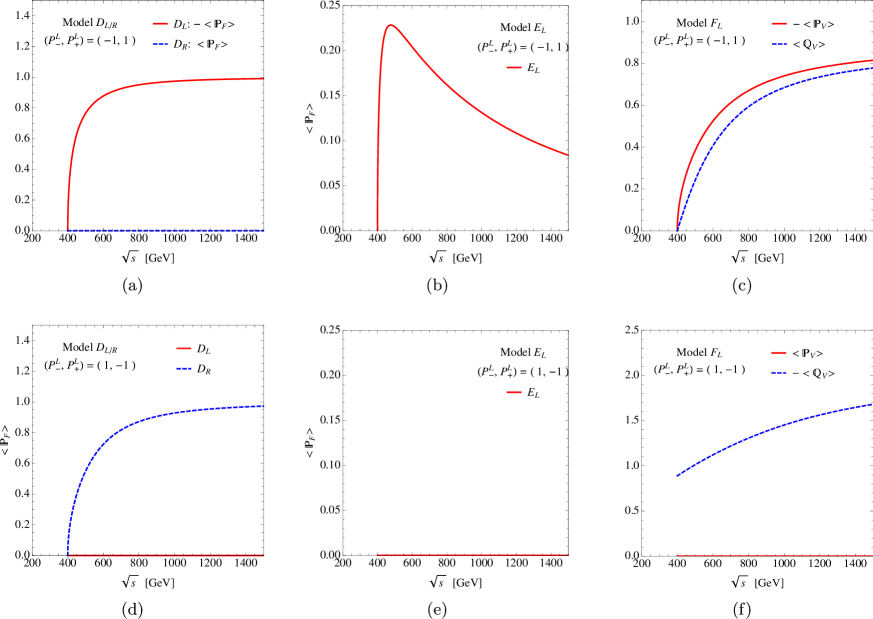
Figure 7: Energy dependence of the coefficients ${\langle\mathbb{P}_{F,V}\rangle}$ and ${\langle\mathbb{Q}_{V}\rangle}$ for a first KK electron ($D_{L/R}$), for a spin-1/2 charged wino ($E_{L}$), and for a spin-1 charged first KK $W$-boson ($F_{L}$). The upper (lower) frames are for left-handed (right-handed) electron and right-handed (left-handed) positron beams, respectively.

It is evident from Eqs. (6.14) and (6.15) that the single polar-angle distributions are isotropic as in the scalar case if the relative chiralities, $\xi_{\rm fs}$ and $\xi_{\rm fv}$, are zero, i.e. the couplings for the decays, $F^{-}_{p}\to\ell^{-}\bar{S}^{0}_{d}$ and $F^{-}_{p}\to\ell^{-}\bar{V}^{0}_{d}$, are pure scalar-type and pure vector-type. In the latter decay mode, not only the relative chirality but also the dilution factor $\eta_{\rm fv}$ must not be zero, i.e, $M_{F_{p}}\neq\sqrt{2}M_{V_{d}}$. Furthermore, as mentioned before, the $P$-odd polarization observable $\langle\mathbb{P}_{F}\rangle$ needs to be non-zero in both of the decay modes, for any non-trivial single decay polar-angle distributions.

Before presenting the single decay polar-angle distributions at a fixed c.m. energy $\sqrt{s}=500$  GeV, we investigate the energy and polarization dependence of the $P$-odd polarization observable $\langle\mathbb{P}_{F}\rangle$ in the $C_{L/R},\,D_{L/R}$ and $E_{L}$ scenarios of spin-1/2 particles.

• Firstly, we note that the polarization observable is identically zero, independently of beam polarization, in the $C_{L/R}$ scenario for the production of a first KK-muon pair $\mu^{+}_{1}\mu^{-}_{1}$, because the coupling of the $Z$ as well as $\gamma$ to the first KK muon pair in the $s$-channel exchange diagram is of a pure vector-type, generating no $P$-violating effects, so that the single decay polar-angle distribution is isotropic as in the spin-0 scalar-pair production. Therefore, the single decay polar-angle distribution cannot be exploited for distinguishing the spin-1/2 case of a first KK muon pair from the spin-0 case of a smuon pair.

• In contrast, as the production of a first KK electron pair occurs through the $t$-channel spin-1 vector-boson contributions with pure left-chiral ($D_{L}$) or right-chiral ($D_{R}$) $ee_{1}V^{0}_{t}$ couplings with the first KK vector boson $V^{0}_{t}=B_{1},\,W^{0}_{1}$ as well as the $s$-channel $\gamma$ and $Z$-boson contributions with pure vector couplings with $F^{\pm}_{p}$, the $P$-odd polarization observable depends strongly on the c.m. energy and beam polarizations. As the c.m. energy increases, the $t$-channel contributions with maximally $P$-violating couplings become dominant rapidly due to the exchange of spin-1 neutral vector bosons $B_{1}$ and $W^{0}_{1}$ so that the $P$-odd observable approaches its maximum value of unity in magnitude in the $D_{L}$ ($D_{R}$) scenario for left-handed (right-handed) electron and right-handed (left-handed) positron polarizations. In the former and latter cases ($D_{L}$ and $D_{R}$), the observable is negative and positive, respectively. On the other hand, for the opposite combination of beam polarizations the observable is zero because the $t$-channel contributions are killed. These features are clearly demonstrated in Figs. 7(a) and (d).

• In the charged wino case ($E_{L}$), the $t$-channel diagram is mediated by a spin-0 electron sneutrino $\tilde{\nu}_{e}$, killing the amplitude effectively in the forward direction due to chirality flipping. As a result, the $P$-odd observable decreases in size as the c.m. energy increases. Moreover, as the $e\tilde{\nu}_{e}\tilde{W}$ coupling is purely left-chiral, the $P$-odd observable is zero for right-handed electron and left-handed positron polarizations. These features can be verified with the plots in Figs. 7(b) and (e).

It is necessary to compare these features of the spin-1/2 $F^{\pm}_{p}$ cases to those for the spin-1 $V^{\pm}_{p}$ cases.

When the parent particle $\mathcal{P}^{\pm}$ is a spin-1 vector boson $V^{\pm}_{p}$, the correlated polar-angle distributions and the normalized lepton polar-angle distribution are given in terms of the $V^{\pm}_{p}$ helicity-dependent production cross sections by

$$\frac{d\sigma^{V}[V^{-}_{p}\to\ell^{-}\bar{F}^{0}_{d}]}{d\cos\theta\,d\cos\theta_{-}} = \frac{d\sigma^{V}}{d\cos\theta}\,\cdot\frac{1}{2}\left[1+\frac{3}{2}\,\xi_{\rm vf}\,\eta_{\rm vf}\,\mathbb{P}_{V}\,\cos\theta_{-}+\frac{1}{2}(3\eta_{\rm vf}-2)\,\mathbb{Q}_{V}\,\frac{(3\cos^{2}\theta_{-}-1)}{2}\right]$$ (6.23)

$$\frac{1}{{\cal C}_{\rm vf}}\frac{d{\cal C}_{\rm vf}}{d\cos\theta_{-}} = \frac{1}{2}\left[1+\frac{3}{2}\,\xi_{\rm vf}\,\eta_{\rm vf}\,\langle\mathbb{P}_{V}\rangle\,\cos\theta_{-}+\frac{1}{2}(3\eta_{\rm vf}-2)\,\langle\mathbb{Q}_{V}\rangle\,\frac{(3\cos^{2}\theta_{-}-1)}{2}\right]$$ (6.24)

with a relative chirality $\xi_{\rm vf}$ and a dilution factor $\eta_{\rm vf}$ defined by

$$\xi_{\rm vf} = \frac{|d^{\ell V}_{F+}|^{2}-|d^{\ell V}_{F-}|^{2}}{|d^{\ell V}_{F+}|^{2}+|d^{\ell V}_{F-}|^{2}}$$ (6.25)

$$\eta_{\rm vf} = \frac{2M^{2}_{V_{p}}}{2M^{2}_{V_{p}}+M^{2}_{F_{d}}}$$ (6.26)

with its minimum value of $\eta^{\rm min}_{\rm vf}=2/3$ for $M_{V_{p}}=M_{F_{d}}$, where the differential cross section and two polarization observables $\mathbb{P}_{V}$ and $\mathbb{Q}_{V}$ are defined by

$$\frac{d\sigma^{V}}{d\cos\theta} = \frac{d\sigma^{V}(\lambda_{-}=+)}{d\cos\theta}+\frac{d\sigma^{V}(\lambda_{-}=-)}{d\cos\theta}+\frac{d\sigma^{V}(\lambda_{-}=0)}{d\cos\theta}$$ (6.27)

$$\mathbb{P}_{V} = \left[\frac{d\sigma^{V}(\lambda_{-}=+)}{d\cos\theta}-\frac{d\sigma^{V}(\lambda_{-}=-)}{d\cos\theta}\right]\bigg{/}\frac{d\sigma^{V}}{d\cos\theta}$$ (6.28)

$$\mathbb{Q}_{V} = \left[\frac{d\sigma^{V}(\lambda_{-}=+)}{d\cos\theta}+\frac{d\sigma^{V}(\lambda_{-}=-)}{d\cos\theta}-2\frac{d\sigma^{V}(\lambda_{-}=0)}{d\cos\theta}\right]\bigg{/}\frac{d\sigma^{V}}{d\cos\theta}$$ (6.29)

and the averages of two polarization observables over the polar-angle distribution are given by

$$\langle\mathbb{P}_{V}\rangle = \frac{1}{\sigma}\int^{1}_{-1}\mathbb{P}_{V}\frac{d\sigma^{V}}{d\cos\theta}\,d\cos\theta=\left(\mathbb{p}^{++}_{++}+\mathbb{p}^{+0}_{+0}+\mathbb{p}^{+-}_{+-}\right)-\left(\mathbb{p}^{-+}_{-+}+\mathbb{p}^{-0}_{-0}+\mathbb{p}^{--}_{--}\right)$$ (6.30)

$$\langle\mathbb{Q}_{V}\rangle = \frac{1}{\sigma}\int^{1}_{-1}\mathbb{Q}_{V}\frac{d\sigma^{V}}{d\cos\theta}\,d\cos\theta=\left(\mathbb{p}^{++}_{++}+\mathbb{p}^{+0}_{+0}+\mathbb{p}^{+-}_{+-}\right)+\left(\mathbb{p}^{-+}_{-+}+\mathbb{p}^{-0}_{-0}+\mathbb{p}^{--}_{--}\right)-2\left(\mathbb{p}^{0+}_{0+}+\mathbb{p}^{00}_{00}+\mathbb{p}^{0-}_{0-}\right)$$ (6.31)

satisfying the inequality conditions $|\langle\mathbb{P}_{V}\rangle|\leq 1$ and $|\langle\mathbb{Q}_{V}\rangle|\leq 2$ in terms of the $3\times 3$ normalized production tensor matrix $\mathbb{p}$ defined similarly to the equation (6.22).

Clearly, only if the vector boson $V^{-}_{p}$ is unpolarized, i.e. the production cross section for each $V^{-}_{p}$ is identical with $d\sigma^{V}(\lambda_{-}=+)=d\sigma^{V}(\lambda_{-}=-)=d\sigma^{V}(\lambda_{-}=0)$, will the decay polar-angle distribution be isotropic. Note that, even if there are no parity-violating effects, i.e. $d\sigma^{V}(\lambda_{-}=+)=d\sigma^{V}(\lambda_{-}=-)$, in the production process, there can exist a non-trivial lepton polar-angle distribution proportional to $3\cos^{2}\theta_{-}-1$, unless the averaged degree of longitudinal polarization $P_{L}(V^{-}_{p})=\sigma^{V}(\lambda_{-}=0)/\sigma^{V}$ of the particle $V^{-}_{p}$ is identical to $1/3$. These properties are demonstrated by the plots in Figs. 7(c) and (f) for the production of a charged first KK $W$-boson pair with $s$-channel $\gamma,Z$ exchanges with pure vector-type couplings and $t$-channel spin-1/2 first KK neutrino exchange with a pure left-chiral coupling. Firstly, as the right-handed electron and left-handed positron polarizations kill the $t$-channel contributions, the $P$-odd observable $\langle\mathbb{P}_{V}\rangle$ is vanishing so that there is no term linear in $\cos\theta_{-}$. Even in this case the $P$-even polarization observable $\langle\mathbb{Q}_{V}\rangle$ survives and increases in size as the c.m. energy increases as shown in Figs. 7(f). Secondly, for the left-handed electron and right-handed positron polarizations, the $P$-violating $t$-channel contribution survives and both the $P$-even and $P$-odd observables increase in size as the c.m. energy increases as shown in Figs. 7(c).

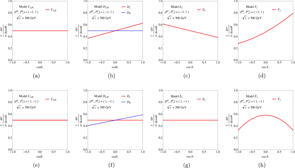
Figure 8: Normalized single decay polar-angle distributions for a spin-1/2 charged first KK muon $\mu^{-}_{1L/1R}$ ($C_{L/R}$) and first KK electron $e^{-}_{1L/1R}$ ($D_{L/R}$), for a spin-1/2 charged wino $\tilde{W}^{-}$ ($E_{L}$) and for a spin-1 charged first KK $W$-boson $W^{-}_{1}$ ($F_{L}$), pair produced with its anti-particle in $e^{+}e^{-}$ collisions at a fixed c.m. energy of 500 GeV. The upper (lower) frames are for left-handed (right-handed) electron and right-handed (left-handed) positron beams.

Figure 8 shows the normalized single decay polar-angle distributions for a spin-1/2 negatively charged first KK muon $\mu^{-}_{1L/1R}$ ($C_{L/R}$) and first KK electron $e^{-}_{1L/1R}$ ($D_{L/R}$), for a spin-1/2 negatively charged wino $\tilde{W}^{-}$ ($E_{L}$) and for a spin-1 negatively charged first KK $W$-boson $W^{-}_{1}$ ($F_{L}$), pair produced with its anti-particle in $e^{+}e^{-}$ collisions at a fixed c.m. energy of 500 GeV.

• As shown in Figs. 8(a) and (e), the distribution for the $\mu^{-}_{1}$ decay is flat because the couplings of both $\gamma$ and $Z$ to the $\mu^{+}_{1}\mu^{-}_{1}$ pair are pure vector-type, preserving parity ($P$).

• Similarly the flat distributions appear for the left-handed (right-handed) KK electron with right-handed (left-handed) electron and left-handed (right-handed) positron polarizations as shown by a (blue) dashed line in Figs. 8(b) and a (red) solid line in Figs. 8(f), as in both cases the $P$-violating $t$-channel contributions are killed. The same flat distribution in the $\tilde{W}$ decay occurs for right-handed electron and left-handed positron beams, killing the $t$-channel sneutrino contribution, as shown in Figs. 8(g).

• There exist non-trivial decay polar-angle distributions with a positive slope in the $e^{-}_{1L/1R}$ decay for left-handed/right-handed electron and right-handed/left-handed positron beams as shown by the red solid line in Figs. 8(b) and by the blue dashed line in Figs. 8(f). This is due to the fact that both the $P$-odd polarization observable $\langle\mathbb{P}_{F}\rangle$ and the relative chirality factor $\xi_{\rm fv}$ is negative and positive for the $e^{-}_{1L}$ and $e^{-}_{1R}$ decay, respectively, so that the product of two quantities is positive in both cases. In contrast, in the $E_{L}$ case with left-handed electron and right-handed positron beams, the $P$-odd polarization observable is positive but the relative chirality $\xi_{\rm fs}$ is negative so that the slope determined by the product of two quantities is negative as shown in Figs. 8(c).

• Finally, in the $F_{L}$ case for a spin-1 negatively charged first KK $W$-boson $W^{-}_{1}$ decay, the lines are clearly curved instead of being straight, as shown in Figs. 8(d) and (h). In particular, even though the coupling of $\gamma$ and $Z$ to a $W^{\pm}_{1}$ pair is $P$-conserving so that the $P$-odd observable $\langle\mathbb{P}_{V}\rangle$ vanishes for right-handed electron and left-handed positron beams, the single decay polar-angle distribution takes a non-trivial quadratic curve shape due to non-vanishing $P$-even polarization observable $\langle\mathbb{Q}_{V}\rangle$.

To summarize. It is necessary to have $P$-violating decays for any non-trivial single decay polar-angle distribution. Moreover, in the spin-1/2 case, the production process must have $P$-violating contributions due to the presence of $P$-violating interactions which can be greatly enhanced by initial beam polarizations. In the spin-1 case, in addition to the $P$-odd polarization observable, there can exist a $P$-even polarization observable leading to non-trivial decay polar-angle distribution, the shape of which is quadratic in $\cos\theta_{\mp}$.

6.5 Angular correlations of two charged leptons

As can be checked with Eqs. (6.14) and (6.15), the lepton polar-angle distribution of the process $e^{-}e^{+}\to F^{-}_{p}F^{+}_{p}$ followed by the decay $F^{-}_{p}\to\ell^{-}S^{0}_{d}$ or $\ell^{-}V^{0}_{d}$ is isotropic if the integration of the polarization observable $\mathbb{P}_{F}$ over the polar-angle $\theta$ is vanishing as in the KK muon-pair production due to the pure vector coupling of the photon and $Z$ boson to the KK muon pair. Therefore, a single lepton angle distribution cannot be exploited to distinguish the spin-1/2 case from the spin-0 case. In this situation, we can exploit the angular correlations of two charged leptons.

6.5.1 Polar-angle correlations

As the spin-1 case can usually be distinguished from the spin-0 and spin-1/2 cases through the coefficient proportional to $(3\cos^{2}\theta_{-}-1)$ even when either the $P$-odd observable $\langle\mathbb{P}_{F}\rangle$ or the $P$-odd relative chirality is vanishing. On the contrary, in the spin-1/2 case there can exist a non-trivial single lepton polar-angle distribution only when both the $P$-odd coefficients and the $P$-odd integral are non-vanishing. Otherwise, the spin-1/2 case cannot be distinguished from the spin-0 case by the single lepton angular distribution. In this $P$-invariant case, we can consider the polar-angle correlation of two final leptons, which is a $P$-even quantity. In general, the polar-angle correlation in the spin-1/2 case can be decomposed into four parts as

$$\frac{1}{{\cal C}_{D}}\frac{d{\cal C}_{D}}{d\cos\theta_{-}d\cos\theta_{+}}\!=\!\frac{1}{4}\left\{1\!+\!\xi_{D}\eta_{D}\left[(\cos\theta_{-}\!+\!\cos\theta_{+})\,\Theta_{F1}+(\cos\theta_{-}\!-\!\cos\theta_{+})\,\Theta_{F2}\right]+\xi^{2}_{D}\eta^{2}_{D}\,\cos\theta_{-}\cos\theta_{+}\,\Theta_{F3}\right\}$$ (6.32)

with $\xi_{D}=\xi_{\rm fs},\,\xi_{\rm fv}$ and $\eta_{D}=1,\,\eta_{\rm fv}$ for the decay modes, $F^{-}_{p}\to\ell^{-}S^{0}_{d},\,\ell^{-}V^{0}_{d}$, respectively. Here, the $P$-odd coefficients, $\Theta_{F1,F2}$, and the $P$-even coefficient $\Theta_{F3}$, which are in general dependent on the $e^{+}e^{-}$ c.m. energy and beam polarizations, are given by

$$\Theta_{F1} = \mathbb{p}^{++}_{++}-\mathbb{p}^{--}_{--}$$ (6.33)

$$\Theta_{F2} = \mathbb{p}^{+-}_{+-}-\mathbb{p}^{-+}_{-+}$$ (6.34)

$$\Theta_{F3} = \left(\mathbb{p}^{+-}_{+-}+\mathbb{p}^{-+}_{-+}\right)-\left(\mathbb{p}^{++}_{++}+\mathbb{p}^{--}_{--}\right)$$ (6.35)

We note in passing that the $P$-odd quantity $\langle\mathbb{P}_{F}\rangle$ appearing in the single lepton polar-angle $\theta_{-}$ distributions is identical to the sum $\Theta_{F1}+\Theta_{F2}$. An identical relation is valid also for the $P$-odd quantity $\langle\mathbb{P}_{V}\rangle$ in the spin-1 case.

Figure 9: Energy dependence of the coefficients $\Theta_{F2}$ and/or $\Theta_{F3}$ of the correlated decay polar-angle distributions for a spin-1/2 charged first KK-muon ($C_{L/R}$) and first KK-electron ($D_{L/R}$) and for a spin-1/2 charged wino ($E_{L}$). The lines in the upper (lower) frames are for left-handed (right-handed) electron and right-handed (left-handed) positron beams, respectively.

As indicated in the previous subsection, the $P$-odd quantities $\Theta_{F1,F2}$ are vanishing in the production of a first KK-muon $\mu^{\pm}_{1L/1R}$ pair, because the coupling of the spin-1 vector bosons $\gamma,Z$ to the first KK-muon pair is of a pure vector type. However, the coefficient $\Theta_{F3}$ defining the $P$-conserving decay polar-angle correlation in Eq. (6.32) is $P$-even so that this quantity does not have to be vanishing even in the $P$-conserving case. As shown numerically by the (red) solid lines in Figs. 9(a) and (d), the $P$-even coefficient $\Theta_{F3}$ increases in size as the c.m. energy increases. As a consequence, it is evident that the spin-1/2 $\mu^{\pm}_{1}$ case can be distinguished from the spin-0 $\tilde{\mu}^{\pm}_{L/R}$ case through the non-trivial polar-angle correlation, which can be significant for pure right-chiral or left-chiral decays with $\xi_{\rm fv}=\pm 1$ and a sizable dilution factor $\eta_{\rm fv}$. We note in passing that the $P$-even coefficients in the other spin-1/2 cases ($D_{L/R}$ and $E_{L}$) in Figs. 9(b), (e), (c)and (f) are also increasing in size with the c.m. energy and already sizable at the c.m. energy of 500 GeV.

6.5.2 Azimuthal-angle correlations

In this subsection, we study the fully-correlated azimuthal-angle distributions in the production of a $\mathcal{P}^{+}\mathcal{P}^{-}$ pair in $e^{+}e^{-}$ collisions and both of their sequential two-body decays $\mathcal{P}^{-}\to\ell^{-}\mathcal{\bar{D}}^{0}$ and $\mathcal{P}^{+}\to\ell^{+}\mathcal{D}^{0}$. The azimuthal-angle difference $\phi=\phi_{-}-\phi_{+}$ under consideration is the angle between the two decay planes, which is invariant under any Lorentz boost along the $\mathcal{P}^{\pm}$ flight direction. These distributions develop through quantum interference between the different helicity states in a coherent sum, indicating that the effect is diluted as the $e^{+}e^{-}$ c.m. energy increases. By extracting this angular dependence, we can determine which helicity states contribute to the sum, and thus we can extract useful information on the spin of the pair-produced particles in a model-independent wayBuckley:2008eb .

The general form of the azimuthal-angle correlation for the production and decays of a spin $J$ particle pair is

$$\frac{1}{\cal C}\frac{d{\cal C}}{d\phi}=\frac{1}{2\pi}\left[1+\mathbb{A}_{1}\cos(\phi)+\cdots+\mathbb{A}_{2J}\cos(2J\phi)\right]$$ (6.36)

We emphasize that the expression is still valid even in a $CP$-noninvariant theory as all the sine terms are washed out by taking the average over two possible production azimuthal angles, which is unavoidable due to a twofold ambiguity in reconstructing the $\mathcal{P}^{\pm}$ momentum directions as shown in Eq. (D.24) in Appendix D. Each coefficient $\mathbb{A}_{i}$ ($i=1$-$2J$) can be worked out from the standard rules of constructing matrix elements, as explicitly described below for the spin-1/2 and spin-1 cases.

Evidently, the correlated azimuthal-angle distribution for a spin-0 scalar-pair production process is flat due to the absence of any production-decay spin correlations. In contrast, the azimuthal-angle distribution for the spin-1/2 fermion-pair production process is given by

$$\frac{1}{{\cal C}_{D}}\frac{d{\cal C}_{D}}{d\phi}=\frac{1}{2\pi}\,\left[1-\xi^{2}_{D}\eta^{2}_{D}\,\Phi_{F}\cos\phi\right]$$ (6.37)

in terms of a $C$-even and $P$-even quantity $\Phi_{F}$ defined as

$$\Phi_{F}=\frac{\pi^{2}}{16}\,{\rm Re}(\mathbb{p}^{++}_{--}+\mathbb{p}^{--}_{++})$$ (6.38)

with $\xi_{D}=\xi_{\rm fs},\xi_{\rm fv}$ and $\eta_{D}=1,\eta_{\rm fv}$ for $\mathcal{D}^{0}=S^{0}_{d}$ and $V^{0}_{d}$, respectively, and the super/sub-scripts $\pm$ for the helicities $\pm 1/2$ of the spin-1/2 fermion $F^{\pm}_{p}$. On the other hand, the correlated azimuthal-angle distribution for a spin-1 vector boson pair $V^{+}_{p}V^{-}_{p}$ consists of three parts as

$$\frac{1}{{\cal C}_{\rm vf}}\frac{d{\cal C}_{\rm vf}}{d\phi}=\frac{1}{2\pi}\left[1-\xi^{2}_{\rm vf}\eta^{2}_{\rm vf}\,\Phi_{V1}\,\cos\phi+(3\eta_{\rm vf}-2)^{2}\,\Phi_{V2}\,\cos(2\phi)\right]$$ (6.39)

in terms of two $C$-even and $P$-even quantities $\Phi_{V1}$ and $\Phi_{V2}$ defined as

$$\Phi_{V1} = \frac{9\pi^{2}}{64}\,{\rm Re}(\mathbb{p}^{++}_{00}+\mathbb{p}^{00}_{--}+\mathbb{p}^{+0}_{0-}+\mathbb{p}^{0+}_{-0})$$ (6.40)

$$\Phi_{V2} = \frac{1}{4}\,{\rm Re}(\mathbb{p}^{++}_{--}+\mathbb{p}^{--}_{++})$$ (6.41)

where the super/sub-scripts $\pm,0$ stand for the helicities, $\pm 1,0$ of the spin-1 vector bosons $\mathcal{P}^{\pm}$. We note that the two-body decays do not suppress the $\cos\phi$ terms, while the highest $\cos(2\phi)$ mode may be suppressed if the polarization analyzing power $\eta_{\rm vf}$ is $2/3$, satisfied only when the parent and daughter particles, $V^{\pm}_{p}$ and $F^{0}_{d}$, are nearly degenerate.

Conceptually, any azimuthal-angle correlation, which is a pure quantum-mechanical effect, requires non-trivial interference among helicity amplitudes with different helicity assignments as indicated by Eqs. (6.38), (6.40) and (6.41) and so they tend to diminish as the c.m. energy increases, as demonstrated numerically in Figs. 10.

• Numerically, the quantity $\Phi_{F}$ takes a value roughly between 0.1 and 0.2 at $\sqrt{s}=500\,{\rm GeV}$ and sensitive to initial beam polarization for the processes with chiral $t$-channel contributions ($D_{L/R}$ and $E_{L}$) as shown in Figs. 10(b), (c), (f) and (g), while it is independent of beam polarization in the production for a charged first KK muon pair $\mu^{\pm}_{1L/1R}$ ($C_{L/R}$) with no $t$-channel contributions as shown in Figs. 10(a) and (d).

• One noteworthy aspect in the spin-1 case ($F_{L}$) is that the quantity $\Phi_{V2}$ is too small (less than 2 %) in magnitude to distinguish the spin-1 $W^{\pm}_{1}$ state from the spin-1/2 states, $\mu^{\pm}_{1},\,e^{\pm}_{1}$ or $\tilde{W}^{\pm}$ as shown in Figs. 10(d) and (h). This strong suppression in the spin-1 $W^{\pm}_{1}$ case is due to the cancellation of the corresponding production helicity amplitudes ($\sim M^{2}_{W^{\pm}_{1}}/E^{2}_{\rm cm}$) that is forced by the relations satisfied for saving the tree-level unitarity.

• On the other hand, the coefficient $\Phi_{V1}$ in the $\cos\phi$ term is sufficiently large so that this correlation can be exploited for distinguishing the spin-1 case at least from the spin-0 case as indicated by the solid lines in Figs. 10(d) and (h).

To summarize. The fully-correlated azimuthal-angle correlations encoding quantum interference between different helicity final states can provide a supplementary but not complete method for spin measurements.

Figure 10: Energy dependence of the coefficients $\Phi_{F}$ and $\Phi_{V1,V2}$ for correlated decay azimuthal-angle distributions for a spin-1/2 charged first KK-muon pair $\mu^{\pm}_{1L/1R}$ ($C_{L/R}$) and first KK-electron pair $e^{\pm}_{1L/1R}$ ($D_{L/R}$), for a spin-1/2 charged wino pair $\tilde{W}^{\pm}$ ($E_{L}$) and for a spin-1 charged first KK-$W$ $W^{\pm}_{1}$ ($F_{L}$). The lines in the upper (lower) frames are for left-handed (right-handed) electron and right-handed (left-handed) positron beams, respectively.

Based on the mass spectrum (6.2) leading to the dilution factor $\eta_{\rm fv}=1/3$ (obtained by substituting these masses into Eq. (6.18)) while $\eta_{\rm fs}=1$, we show in Figs. 11 the fully-correlated azimuthal-angle distributions for a spin-1/2 charged first KK muon and electron ($C_{L/R}$ and $D_{L/R}$), for a spin-1/2 charged wino ($E_{L}$) and for a spin-1 charged first KK $W$-boson ($F_{L}$). The plots in the upper (lower) frames are for left-handed (right-handed) electron and right-handed (left-handed) positron beams, respectively.

• In the first KK muon and electron cases ($C_{L/R}$ and $D_{L/R}$), the azimuthal-angle correlations are too small to be distinguished from the flat distribution in the spin-0 case as shown in Figs. 11(a), (b), (e) and (f). This tiny correlation is owing to the fact that we have a small coefficient $\Phi_{F}$ but also a small dilution factor $\eta^{2}_{\rm fv}=1/9$, which can be much larger for a small mass ratio of the parent and daughter particles.

• In contrast the spin-1/2 charged wino case ($E_{L}$) shows a rather distinct azimuthal-angle correlation as the dilution factor $\eta_{\rm fs}=1$ independently of particle masses, as shown in Figs. 11(c) and (g).

• In the spin-1 case the dilution factor is $\eta_{\rm vf}=8/9$ and the coefficient $\Phi_{V1}$ in the $\cos\phi$ term is between 0.4 and 0.6 in magnitude while the coefficient $\Phi_{V2}$ is extremely tiny. As a consequence, the azimuthal-angle correlation exhibits a distinct distribution proportional to $1+\alpha_{1}\cos\phi+\alpha_{2}\cos 2\phi$ with $\alpha_{1}\sim 0.25$ and $\alpha_{2}\sim 0$, as shown in Figs. 11(d) and (h).

To summarize. We have shown for the mass spectrum (6.2) that the spin-1/2 KK muons and electrons cannot be so easily distinguished from the spin-0 smuons and selectrons through the azimuthal-angle correlation. In contrast, the spin-1/2 charged wino case and the spin-1 KK $W$-boson case can be distinguished from the spin-0 cases. However, it turned out to be difficult to establish the spin-1 nature of the KK $W$-boson due to the strong suppression of the $\cos 2\phi$ mode, requiring other methods such as the decay polar-angle distributions.

Figure 11: Correlated azimuthal-angle distributions for a spin-1/2 charged first KK-muon and KK-electron ($C_{L/R}$ and $D_{L/R}$), for a spin-1/2 charged wino ($E_{L}$) and for a spin-1 charged first KK-$W$ ($F_{L}$). The upper (lower) frames are for left-handed (right-handed) electron and right-handed (left-handed) positron beams.

6.6 Effects of ISR, beamstrahlung, particle widths and kinematic cuts

In this subsection for a more realistic investigation we study the impact on the various kinematic observables by initial state radiation (ISR) Skrzypek:1990qs , beamstrahlung Chen:1991wd and finite width of the particle $\mathcal{P}^{\pm}$ as well as typical kinematic cuts in an $e^{+}e^{-}$ collider environment. We use FeynRules Christensen:2008py ; Christensen:2009jx ; Alloul:2013bka to implement all the vertices and propagators into the format of CalcHEP Belyaev:2012qa . Then, we perform extensive simulations for the spin and chirality assignments listed in Tab. 3.

The kinematic cuts taken in the present numerical analysis are

$$|\cos\theta_{\ell}|\,<\,0.9962\quad\mbox{and}\quad E_{\ell}\,>\,10\,{\rm GeV}$$ (6.42)

to ensure detection, where $\theta_{\ell}$ and $E_{\ell}$ are the polar angle and the energy of the lepton in the laboratory frame, and

$$\not\!{p}_{T}\,>\,10\,{\rm GeV}$$ (6.43)

to remove the background from $e^{+}e^{-}\to e^{+}e^{-}\ell^{+}\ell^{-}$ where the final $e^{+}e^{-}$ pair is missed. The $\mathcal{P}$ total width $\Gamma_{\mathcal{P}}$ is calculated to be the sum of the partial widths of the two decays $\mathcal{P}^{-}\to\ell^{-}\mathcal{\bar{D}}^{0}$ with $\ell=e$ and/or $\mu$, for a simple analysis of the impact of the width. ISR and Beamstrahlung effects at ILC are calculated with CalcHEP using parameters in Tab. 5 Phinney:2007gp .

Collider	$E_{\rm cm}$ ($\sqrt{s}$) [GeV]	$N$ [$10^{10}$]	$\sigma_{x}$ [nm]	$\sigma_{y}$ [nm]	$\sigma_{z}$ [$\mu$m]
ILC	500	2	640	5.7	300

Table 5: Key parameters of the initial beams at the ILC used in our numerical analysis. Here $N$ is the number of particles per bunch, $\sigma_{x,y}$ are the RMS beam sizes at the interaction point, and $\sigma_{z}$ is the RMS bunch length.

Figure 12: Excitation curve of the cross section close to threshold for the production of a spin-0 charged $R$-selectron pair $\tilde{e}^{\pm}_{R}$ ($B_{R}$), a spin-1/2 charged $R$-type first KK-electron pair $\tilde{e}^{\pm}_{R}$ ($D_{R}$), a spin-1/2 charged wino pair $\tilde{W}^{\pm}$ ($E_{L}$) or a spin-1 charged first KK-$W$ pair $W^{\pm}_{1}$ ($F_{L}$) close to threshold including ISR, beamstrahlung and width effects as well as the kinematic cuts in Eqs. (6.42) and (6.43); the statistical errors correspond to $\mathcal{L}=10\,{\rm fb}^{-1}$ per point. The initial beams are set to be unpolarized in the frames, (a), (b), (d) and (e), while the electron (positron) beams are purely left-handed (right-handed) and purely right-handed (left-handed) in the frames, (c) and (f).

Rather than listing all the scenarios studied in the previous subsections, we present our simulation results for only a few typical scenarios selected for each observable. Figs. 12 shows the excitation curve of the production of a spin-0 charged $R$-selectron pair $\tilde{e}^{\pm}_{R}$ ($B_{R}$), a spin-1/2 charged $R$-type first KK-electron pair $\tilde{e}^{\pm}_{R}$ ($D_{R}$), a spin-1/2 charged wino pair $\tilde{W}^{\pm}$ ($E_{L}$) or a spin-1 charged first KK $W$-boson pair $W^{\pm}_{1}$ ($F_{L}$) close to threshold after the ISR, beamstrahlung and width effects as well as the kinematic cuts in Eqs. (6.42) and (6.43) are included. The statistical errors correspond to $\mathcal{L}=10\,{\rm fb}^{-1}$ per point. Except for Figs. 12(c) and (f), the initial electron and positron beams are taken to be unpolarized. The plot of the upper (lower) right frame is for left-handed (right-handed) electron and right-handed (left-handed) positron beams.

• The production cross section can take a finite value even below threshold as the particle can be produced virtually with a mass smaller than its on-shell mass due to its non-zero width, as indicated by the tail extended toward the lower energy region in each frame. Adjusting the width effect, it is evident that for unpolarized beams the spin-0 scalar production process ($B_{R}$) exhibits a slow $P$-wave excitation shown in Figs. 12(a) while the spin-1/2 fermion production processes ($D_{R}$ and $E_{L}$) and the spin-1 vector-boson production process ($F_{L}$) show a sharp $S$-wave excitation, as in Figs. 12(b), (c), (d) and (e).

• In the spin-1 case, if the $t$-channel contribution is killed by complete right-handed electron and left-handed positron polarizations, the cross section rises in slow $P$ waves near threshold in Figs. 12(f). Nevertheless, the number of events is very small so that it is expected to be quite difficult to confirm this $P$-wave pattern quantitatively.

• The threshold behavior is not affected so much by ISR and beamstrahlung effects.

To recapitulate. The spin-0 case can be clearly distinguished from the spin-1/2 and spin-1 cases in the specific scenarios through the threshold scan method, although a new method is required for distinguishing the spin-1 case from the spin-1/2 cases and even from the spin-0 case in the general case, as emphasized before.

Figure 13: The polar-angle distributions with the contribution of false solution for the production of a spin-0 charged $R$-type smuon/selectron pair $\tilde{e}^{\pm}_{R}/\tilde{e}^{\pm}_{R}$ ($A_{R}/B_{R}$), a spin-1/2 charged $R$-type first KK-muon/KK-electron pair $\mu^{\pm}_{1}/e^{\pm}_{1}$ ($C_{R}/D_{R}$), a spin-1/2 charged wino pair $\tilde{W}^{\pm}$ ($E_{L}$) or a spin-1 charged first KK-$W$ pair $W^{\pm}_{1}$ ($F_{L}$), including ISR, beamstrahlung and width effects. Except for the frames, (d) and (e), the initial electron and positron beams are set to be unpolarized. The frames, (d) and (h), are for left-handed (right-handed) and right-handed (left-handed) electron (positron) beams, respectively. The simulation for the polar-angle distribution is based on a fixed number of events $N_{\rm ev}=10^{4}$ at the c.m. energy of 500 GeV.

As shown before, there exists a two-fold discrete ambiguity in determining the $\mathcal{P}^{\pm}$ momentum in the antler-topology event. Therefore, we show in Figs. 13 the polar-angle distributions with the contribution of false solution included for the production of a spin-0 charged $R$-type smuon/selectron pair $\tilde{e}^{\pm}_{R}/\tilde{e}^{\pm}_{R}$ ($A_{R}/B_{R}$), a spin-1/2 charged $R$-type first KK-muon/KK-electron pair $\mu^{\pm}_{1}/e^{\pm}_{1}$ ($C_{R}/D_{R}$), a spin-1/2 charged wino pair $\tilde{W}^{\pm}$ ($E_{L}$) or a spin-1 charged first KK $W$-boson pair $W^{\pm}_{1}$ ($F_{L}$), including ISR, beamstrahlung and width effects as well as the kinematic cuts in Eqs. (6.42) and (6.43). Except for Figs. 13(d) and (h), the initial electron and positron beams are assumed to be unpolarized. The plot of the upper (lower) right-most frame is for left-handed (right-handed) electron and right-handed (left-handed) positron beams. For the simulation we simply take a fixed number of events $N_{\rm ev}=10^{4}$ at the c.m. energy of 500 GeV.

• The $\sin^{2}\theta$ law for the production of spin-0 particles (for $R$-type smuons ($A_{R}$) and $R$-type selectrons ($B_{R}$) close to threshold) is a unique signal for the spin-0 character. This feature can be confirmed in Figs. 13(a) and (b) after the false distribution following the true distribution with a little dilution are extracted out from the sum of the true and false solutions.

• However, the polar-angle distributions in the spin-1/2 and spin-1 cases have so much more involved patterns that it is not straightforward to distinguish the spin-1 case from the spin-1/2 case, unless beam polarizations are exploited.

• In the spin-1 case ($F_{L}$) the polar-angle distribution is quite different for each combination of the electron and positron longitudinal polarizations as shown in Figs. 13(d) and (h). In particular, the true polar-angle distribution in Figs. 13(h) with right-handed electron and left-handed positron polarizations is characteristically different from that for the spin-1/2 first KK muon case ($C_{R}$) shown in Figs. 13(e).

We note that the curve of the false solution is sensitively related not only to the curve of the true solution but also to the chiral structure of the decay processes as clearly shown by the shaded area in Figs. 13(h). This is because the direction of the false solution depends not only on the the direction of the true solution but also on the flight directions of the two leptons, whose distributions are strongly chirality-dependent. Numerically we have confirmed that the curve with a negative slope is due to the pure left-chiral $eW_{1}\nu_{1}$ coupling involved in the decay $W^{-}_{1}\to\ell^{-}\bar{\nu}_{\ell}$. As in the excitation curves, the polar-angle distributions turn out to be not much distorted by the ISR and beamstrahlung effects.

Figure 14: The upper frames are for the single decay polar-angle distribution for the combination of the production of a charged pair $\mathcal{P}^{-}\mathcal{P}^{-}$ and the sequential decay of the negatively-charged particle $\mathcal{P}^{-}\to\ell^{-}\mathcal{\bar{D}}^{0}$ and the lower frames are for the full azimuthal-angle correlations in the antler-topology process. For these distributions, we consider the production of a spin-0 charged $R$-type selectron pair $\tilde{e}^{\pm}_{R}$ ($B_{R}$), a spin-1/2 charged $R$-type first KK-electron pair $e^{\pm}_{1R}$ ($D_{R}$), a spin-1/2 charged wino pair $\tilde{W}^{\pm}$ ($E_{L}$) or a spin-1 charged first KK-$W$ pair $W^{\pm}_{1}$ ($F_{L}$), including ISR, beamstrahlung and width effects as well as the kinematic cuts in Eqs. (6.42) and (6.43). The initial electron and positron beams are assumed to be unpolarized. The simulation for each of the decay polar-angle distributions and azimuthal-angle correlations is based on a fixed number of events $N_{\rm ev}=10^{4}$ at the c.m. energy of $\sqrt{s}=500\,{\rm GeV}$.

Then, let us consider the single decay polar-angle distributions in the combined process of the $\mathcal{P}^{\pm}$ pair production followed by the decay of a negatively-charged particle $\mathcal{P}^{-}\to\ell^{-}\mathcal{\bar{D}}^{0}$ and the decay azimuthal-angle correlations in the antler-topology process in the four scenarios, $B_{R}$ for a spin-0 charged $R$-type selectron pair $\tilde{e}^{\pm}_{R}$, $D_{R}$ for a spin-1/2 charged $R$-type first KK-electron pair $e^{\pm}_{1R}$, $E_{L}$ for a spin-1/2 chargino wino pair $\tilde{W}^{\pm}$ and $F_{L}$ for a spin-1 first KK $W$-boson pair $W^{\pm}_{1}$. The initial electron and positron beams are taken to be unpolarized.

The upper frames of Figs. 14 show the single decay polar-angle distributions after including the ISR, beamstrahlung and width effects as well as the kinematic cuts in Eqs. (6.42) and (6.43) in the four different scenarios ($B_{R}$, $D_{R}$, $E_{L}$ and $F_{L}$). For the hypothetical case that no QED radiation degrades the nominal production energy, since the ratios of the right-handed cross section with $(P^{L}_{-},P^{L}_{+})=(1,-1)$ over the left-handed one with $(P^{L}_{-},P^{L}_{+})=(-1,+1)$ for scenario $B_{R}$, $D_{R}$, $E_{L}$ and $F_{L}$ are $27.4$, $99.8$, $4.51\times 10^{-4}$ and $2.89\times 10^{-4}$ respectively, the distribution should be flat in the scenario $B_{R}$, linear with a positive slope in the scenario $D_{R}$, linear with a negative slope in the scenario $E_{L}$ and quadratic in a downward curved shape in the scenario $F_{L}$ for unpolarized beams, as worked out from the plots in Figs. 8. However, in the more realistic situation that ISR and beamstrahlung decrease the $\mathcal{P}^{+}\mathcal{P}^{-}$ production energy, the angular distribution is no longer linear in the spin-0 and spin-1/2 cases and no longer curved downward in the spin-1 case, as shown in the upper frames of Figs. 14. Considerable depletions are observed at $\cos\theta_{-}\to\pm 1$ when the constraint on $E_{\mathcal{P}^{\pm}}$ tends to be most largely invalidated. However, we note that, since both the ISR spectrum Skrzypek:1990qs and the beamstrahlung spectrum Chen:1991wd can be calculated theoretically and measured precisely, the ISR and beamstrahlung effects can be unfolded from the data, for instance, by applying a bin-by-bin correction or a matrix inversion procedure, although we will not perform the unfolding procedure in the present, rather simple numerical analysis.

The lower frames of Figs. 14 show the full azimuthal-angle correlations in the same set of four scenarios as in the single decay polar-angle distributions. Firstly, it turns out that the ISR, beamstrahlung and width as well as the kinematic cuts do not spoil the azimuthal-angle correlation patterns. The distribution is indeed flat in the angle $\phi$ in the scenario $B_{R}$ for a spin-0 selectron pair and nearly flat in the scenario $D_{R}$ as expected from Figs. 14 (e) and (f). The curves in the spin-1/2 charged wino case ($E_{L}$) and the spin-1 first KK $W$-boson case ($F_{L}$) are consistent with the simple $\cos\phi$ distribution, as shown in Figs. 14(g) and (h). (We fold the range of the angle $\phi$ into $[0,\pi]$ with respect to the line with $\phi=\pi$ for the numerical simulation, as $\phi$ is calculated from $\cos\phi$ which can be determined unambiguously.) We note once more that the coefficient of the $\cos 2\phi$ mode is strongly suppressed due to the relations for restoring tree-level unitarity.

6.7 Influence from ECV interactions

Every numerical analysis performed so far is based on the assumption that electron chirality is preserved (to very good approximation). Although the approximation is valid in the SM with its EW gauge symmetry spontaneously breaking through the BEH mechanism, it may be invalid in the models with additional scalar bosons and with mass generation by different mechanisms. Evidently the ECV terms are already constrained by various low-energy physical quantities. However, the complete analysis of those constraints is very much involved and beyond the scope of the present work. Therefore, before closing this lengthy section, we comment briefly on the possible influence of the ECV terms on the spin determination rather qualitatively, if they are not so strongly suppressed.

As the analytic expressions of production and two-body helicity amplitudes listed in Sects. 3 and 4 indicate, the ECV effects in the production process $e^{+}e^{-}\to\mathcal{P}^{+}\mathcal{P}^{-}$ are generated when a spin-0 scalar $S^{0}_{s}$ couples both to the $e^{+}e^{-}$ pair and also when the $\mathcal{P}^{+}\mathcal{P}^{-}$ pair and/or the $t/u$-channel trilinear vertices involving an electron are non-chiral, i.e. have both left-handed and right-handed couplings while the ECV effects in the decay processes are generated by non-chiral decay trilinear $\mathcal{P}\ell\mathcal{D}$ vertices.

In the ECV case, the electron and positron helicities are identical, $\sigma_{-}=\sigma_{+}$ and they form a $J_{0}=0$ initial two-body state. Therefore, the production polar-angle distribution is isotropic at threshold and the threshold excitation is in a sharp $S$ wave except when a spin-1/2 $F^{+}_{p}F^{-}_{p}$ pair is produced only through an $s$-channel pseudoscalar exchange ($s^{FF}_{S+}=-s^{FF}_{S-}$). As a result, the characteristic patterns of threshold excitation and polar-angle distribution in the ECC case can be spoiled in the presence of the ECV contributions.

If the decay vertices are non-chiral, the relative chirality is not maximal in magnitude any more, i.e. $|\xi|<1$, reducing the production-decay correlation even for the spin-1/2 and spin-1 cases. In the extreme situation with zero relative chirality, there exist no non-trivial decay angular distributions for determining whether the spin of the parent particle $\mathcal{P}$ is 0 or 1/2. In contrast to the spin-1/2 case, there exists a decay-angle distribution independent of the relative chirality in the spin-1 case. Even though the effectiveness of this distribution is reduced by a dilution factor, the spin-1 case can be distinguished from the spin-0 and spin-1/2 cases through the chirality-independent decay-angle correlations Christensen:2013sea .

7 Summary and conclusions

In this paper, we have made a systematic study of kinematic observables connected with the antler-topology process $e^{+}e^{-}\to\mathcal{P}^{+}\mathcal{P}^{-}\to\ell^{+}\ell^{-}\mathcal{D}^{0}\mathcal{\bar{D}}^{0}$ which could serve as model-independent tests for determining the spins of the charged particles $\mathcal{P}^{\pm}$ and the invisible neutral particles $\mathcal{D}^{0}$ and $\mathcal{\bar{D}}^{0}$ as well as the intermediate virtual particles participating in the production process.

It is evident from our analysis that the model-independent determination of the spin quantum numbers of new particles is a complex task even at $e^{+}e^{-}$ colliders with clean and fixed initial-state environments and beam polarizations. The degree of complexity depend crucially on the chiral structures as well as kinematic features of the particles. Not only threshold excitation and angular distributions controlled through initial beam polarizations in pair production but also angular correlations in particle decays provide powerful methods for experimental spin measurements.

The predictions for the threshold excitation and the polar-angle distributions in the production processes, separated into the ECC and ECV parts when the electron is assumed to be massless, are summarized in Tab. 6.

$e^{+}e^{-}$ chiralities	Spin $J_{\mathcal{P}}$	$t$ or $u$ contributions	Threshold excitation	Production polar-angle distribution
	$0$	N	$\beta^{3}$	$\sin^{2}\theta$
		Y	$\beta^{3}$	$\sin^{2}\theta$ at threshold
chirality	$1/2$	N	$\beta$	$1+\kappa_{1/2}\cos^{2}\theta$
conserving		Y	$\beta$	isotropic at threshold
	$1$	N	$\beta^{3}$	$1-\kappa_{1}\cos^{2}\theta$
		Y	$\beta$	isotropic at threshold
	$0$	N	$\beta$	isotropic
		Y	$\beta$	isotropic at threshold
chirality	$1/2$	N	$\beta^{3}/\beta\,[\,{\rm S/P}\,]$	isotropic
violating		Y	$\beta$	isotropic at threshold
	$1$	N	$\beta$	isotropic
		Y	$\beta$	isotropic at threshold

Table 6: The threshold behavior and the polar-angle distribution of the ECC and ECV parts of the production process $e^{+}e^{-}\to\mathcal{P}^{+}\mathcal{P}^{-}$, with [S/P] standing for pure scalar-type or pseudoscalar-type couplings, respectively. Here, the energy-dependent coefficients, $\kappa_{1/2}$ and $\kappa_{1}$, take 0 and 3/19 at threshold and they approach 1 asymptotically at high energies, respectively.

In any theory with conserved chiral symmetry guaranteeing the electron mass to be zero before EWSB such as MSSM and MUED, the ECV parts are connected with the extremely tiny electron mass so that their contributions are negligible for high energy processes. In this ECC case, as shown in the chirality conserving part of Tab. 6, the $\sin^{2}\theta$ law for the production of a spin-0 scalar pair (close to threshold) is a unique signal of the spin-0 character. While the observation of the $\sin^{2}\theta$ polar-angle distribution is sufficient for scalar particles, the $P$-wave $\beta^{3}$ onset of the excitation curve is necessary but not a sufficient condition for the spin-0 character. Nevertheless, we have found that combining the two distributions and using initial beam polarizations to separately diagnose four $e^{+}e^{-}$ helicity combinations enable us not only to determine the $\mathcal{P}$ spin unambiguously but also to get crucial information on the spins of intermediate particles and the chiral structure of the couplings in the ECC case.

If there exist any non-negligible ECV contributions, then the patterns of both threshold excitation and production angle distribution may be qualitatively different from those in the ECC case, as shown in the chirality violating part of Tab. 6. However, one can always use Eq. (3.9) and Eq. (3.11) to extract the ECC part of pair production, as there exists at least a contribution from an $s$-channel photon, to get spin information from threshold excitation and production angle distribution of the ECC part.

Combining the production and decay processes in the antler-topology process, it is possible to construct several correlated observables for a spin-1/2 or spin-1 particle pair $\mathcal{P}^{\pm}$. Evidently there is no production-decay correlation for a spin-0 $\mathcal{P}$, which is a characteristic feature for the spin-0 case. The sensitivities to the $\mathcal{P}$ spin depend strongly on the chiral structure reflected in the production and decay helicity amplitudes and the degrees of initial and final beam polarizations. If the couplings for the decays are pure chiral and the high degree of beam polarizations are available, then the decay polar-angle distributions are very powerful for determining the $\mathcal{P}$ spin as the relative chiralities serving as the polarization analysis powers are maximal. The azimuthal-angle distribution for the difference $\phi$ between the azimuthal angles of two decay planes also provides a supplementary method for determining the $\mathcal{P}$ spin, although this quantum-interference effect diminishes as the c.m. energy increases.

If the decay vertices are not pure chiral, the sensitivities of the kinematic observables to the particle spins are reduced. In the extreme cases of $P$-conserving pure vector or axial vector couplings, we do not have any production-decay correlations in the spin-1/2 case. Even in this case, there exists a non-trivial $P$-even observable in the $\cos 2\phi$ mode in the spin-1 case. However, we have found that the coefficient determined by the production process $e^{+}e^{-}\to V^{+}_{p}V^{-}_{p}$ is strongly suppressed when the specific relations among couplings are satisfied for saving tree-level unitarity at high energies. As a result, it may be very difficult in those extreme cases to determine the spins of the particle involved in the antler-topology process.

To conclude. It is a very complex task to determine the spins of new particles in a model-independent way in a general theory beyond the SM. Nevertheless, we have found that, if electron chirality invariance is valid to very good approximation, the spin of the new particles taking part in the antler-topology process can be determined in a model-independent way through various energy- and angle-dependent observables at $e^{+}e^{-}$ colliders with polarized beams. Any non-chiral contributions, which are expected to be insignificant as in many popular models beyond the SM, render the model-independent spin determination more difficult. However we can still use beam polarizations to extract the chirality-conserving pieces to get useful information on the spins of new particles based on various approaches described in the present work. After all, a high energy $e^{+}e^{-}$ collider with polarized beams is a powerful machine for diagnosing not only the spin but also the chirality structure of new particles, if they are kinematically available.

Acknowledgements. The work of SYC was supported in part by Basic Science Research Program through the National Research Foundation (NRF) funded by the Ministry of Education, Science and Technology (NRF-2011-0010835) and in part by research funds of Chonbuk National University in 2013. NDC was supported in part by PITT PACC and the U.S. Department of Energy under grant No. DE-FG02-95ER40896.

Appendix A Feynman rules for interaction vertices

The initial $e^{+}e^{-}\mathcal{S}^{0}_{s}$ and final $\mathcal{S}^{0}_{s}\mathcal{P}^{+}\mathcal{P}^{-}$ currents for the $s$-channel $\mathcal{S}^{0}_{s}$ exchange diagram contributing to the process $e^{+}e^{-}\to\mathcal{P}^{+}\mathcal{P}^{-}$ with $\mathcal{S}^{0}_{s}=S^{0}_{s}$ or $V^{0}_{s}$ and $\mathcal{P}^{-}=S^{-}_{p},F^{-}_{p}$ or $V^{-}_{p}$ can be parameterized in the following generic form:

$$J^{S}_{ee} \equiv \langle S^{0}_{s}\|e^{-}(p_{-})e^{+}(p_{+})\rangle=e\,\bar{v}(p_{+})\,[s^{S}_{ee+}P_{+}+s^{S}_{ee-}P_{-}]\,u(p_{-})$$ (A.1)

$$J^{V\mu}_{ee} \equiv \langle V^{0}_{s}\|e^{-}(p_{-})e^{+}(p_{+})\rangle^{\mu}=e\,\bar{v}(p_{+})\,[\gamma^{\mu}\,(s^{V}_{ee+}P_{+}+s^{V}_{ee-}P_{-})]\,u(p_{-})$$ (A.2)

$$J^{SS}_{S} \equiv \langle S^{-}_{p}(q_{-})S^{+}_{p}(q_{+})\|S^{0}_{s}\rangle=2eM_{S_{p}}\,s^{SS}_{S}$$ (A.3)

$$J^{SS}_{V\mu} \equiv \langle S^{-}_{p}(q_{-})S^{+}_{p}(q_{+})\|V^{0}_{s}\rangle_{\mu}=e\,s^{SS}_{V}\,(q_{-}-q_{+})_{\mu}$$ (A.4)

$$J^{FF}_{S} \equiv \langle F^{-}_{p}(q_{-})F^{+}_{p}(q_{+})\|S^{0}_{s}\rangle=e\,\bar{u}(q_{-})\,[s^{FF}_{S+}P_{+}+s^{FF}_{S-}P_{-}]\,v(q_{+})$$ (A.5)

$$J^{FF}_{V\mu} \equiv \langle F^{-}_{p}(q_{-})F^{+}_{p}(q_{+})\|V^{0}_{s}\rangle_{\mu}=e\,\bar{u}(q_{-})\,[\gamma^{\mu}(s^{FF}_{V+}P_{+}+s^{FF}_{V-}P_{-})]\,v(q_{+})$$ (A.6)

$$J^{VV}_{S} \equiv \langle V^{-}_{p}(q_{-})V^{+}_{p}(q_{+})\|S^{0}_{s}\rangle=2eM_{V_{p}}\,s^{VV}_{S}\epsilon^{*}_{-}(q_{-})\cdot\epsilon^{*}_{+}(q_{+})$$ (A.7)

$$J^{VV}_{V\mu} \equiv \langle V^{-}_{p}(q_{-})V^{+}_{p}(q_{+})\|V^{0}_{s}\rangle_{\mu}=-e\,s^{VV}_{V}\left[(q_{-}-q_{+})^{\mu}\epsilon^{*}_{-}(q_{-})\cdot\epsilon^{*}_{+}(q_{+})\right.$$ (A.8)

$$\left.\hskip 108.12054pt+2q_{+}\cdot\epsilon^{*}_{-}(q_{-})\epsilon^{*\mu}_{+}(q_{+})-2q_{-}\cdot\epsilon^{*}_{+}(q_{+})\epsilon^{*\mu}_{-}(q_{-})\right]$$

with the chiral projection operators $P_{\pm}=\tfrac{1}{2}(1\pm\gamma_{5})$. In the last expression for the triple-vector vertex, the on-shell conditions $q_{-}\cdot\epsilon^{*}_{-}(q_{-})=q_{+}\cdot\epsilon^{*}_{+}(q_{+})=0$ are imposed.

The $e\mathcal{P}\mathcal{T}$ interaction vertices $T^{e\mathcal{P}}_{\mathcal{T}}$ for the $t$-channel neutral $\mathcal{T}^{0}$-exchange diagrams in the production process $e^{+}e^{-}\,\to\,\mathcal{P}^{+}\mathcal{P}^{-}$ with $\mathcal{P}^{\pm}=S^{\pm}_{p},F^{\pm}_{p}$ or $V^{\pm}_{p}$ and $\mathcal{T}^{0}=S^{0}_{t},F^{0}_{t},V^{0}_{t}$ can be parameterized as follows:

$$T^{eS}_{F} \equiv \langle S^{-}_{p}|F^{0}_{t}|e^{-}\rangle=e\,(t^{eS}_{F+}\,P_{+}+t^{eS}_{F-}\,P_{-})$$ (A.9)

$$T^{eF}_{S} \equiv \langle F^{-}_{p}|S^{0}_{t}|e^{-}\rangle=e\,(t^{eF}_{S+}\,P_{+}+t^{eF}_{S-}\,P_{-})$$ (A.10)

$$T^{eF}_{V\mu} \equiv \langle F^{-}_{p}|V^{0}_{t}|e^{-}\rangle_{\mu}=e\,\gamma_{\mu}\,(t^{eF}_{V+}\,P_{+}+t^{eF}_{V-}\,P_{-})$$ (A.11)

$$T^{eV}_{F\mu} \equiv \langle V^{-}_{p}|F^{0}_{t}|e^{-}\rangle_{\mu}=e\,\gamma_{\mu}\,(t^{eV}_{F+}\,P_{+}+t^{eV}_{F-}\,P_{-})$$ (A.12)

and the $e\mathcal{P}\mathcal{U}$ interaction vertices $U^{e\mathcal{P}}_{\mathcal{U}}$ for the $u$-channel doubly-charged  $\mathcal{U}^{--}$-exchange diagrams can be parameterized as follows:

$$U^{eS}_{F} \equiv \langle S^{+}_{p}|F^{--}_{u}|e^{-}\rangle=e\,(u^{eS}_{F+}\,P_{+}+u^{eS}_{F-}\,P_{-})$$ (A.13)

$$U^{eF}_{S} \equiv \langle F^{+}_{p}|S^{--}_{t}|e^{-}\rangle=e\,(u^{eF}_{S+}\,P_{+}+u^{eF}_{S-}\,P_{-})$$ (A.14)

$$U^{eF}_{V\mu} \equiv \langle F^{+}_{p}|V^{--}_{t}|e^{-}\rangle_{\mu}=e\,\gamma_{\mu}\,(u^{eF}_{V+}\,P_{+}+u^{eF}_{V-}\,P_{-})$$ (A.15)

$$U^{eV}_{F\mu} \equiv \langle V^{+}_{p}|F^{--}_{t}|e^{-}\rangle_{\mu}=e\,\gamma_{\mu}\,(u^{eV}_{F+}\,P_{+}+u^{eV}_{F-}\,P_{-})$$ (A.16)

We note that in the present work, negatively-charged (positively-charged) states are treated as particles (anti-particles), respectively.

The amplitudes for the two-body decay $\mathcal{P}^{-}(q_{-})\to\ell^{-}(p_{1})\mathcal{\bar{D}}^{0}(p_{2})$ and its charge-conjugated process with $\mathcal{P}^{-}=S^{-}_{p},F^{-}_{p}$ or $V^{-}_{p}$ and $\mathcal{\bar{D}}^{0}=\bar{S}^{0}_{d},\bar{F}^{0}_{d}$ or $\bar{V}^{0}_{d}$ can be parameterized in general as follows:

$$D^{\ell F}_{S} \equiv \langle\ell^{-}\bar{F}^{0}_{d}\|S^{-}_{p}\rangle=e\,\bar{u}(p_{1})[d^{\ell F}_{S+}P_{+}+d^{\ell F}_{S-}P_{-}]\,v(p_{2})$$ (A.17)

$$D^{\ell S}_{F} \equiv \langle\ell^{-}\bar{S}^{0}_{d}\|F^{-}_{p}\rangle=e\,\bar{u}(p_{1})[d^{\ell S}_{F+}P_{+}+d^{\ell S}_{F-}P_{-}]\,u(q_{-})$$ (A.18)

$$D^{\ell V}_{F} \equiv \langle\ell^{-}\bar{V}^{0}_{d}\|F^{-}_{p}\rangle=e\,\epsilon^{\mu*}(p_{2})\bar{u}(p_{1})\gamma_{\mu}\,[d^{\ell V}_{F+}P_{+}+d^{\ell V}_{F-}P_{-}]\,u(q_{-})$$ (A.19)

$$D^{\ell F}_{V} \equiv \langle\ell^{-}\bar{F}^{0}_{d}\|V^{-}_{p}\rangle=e\,\bar{u}(p_{1})\gamma_{\mu}\,[d^{\ell F}_{V+}P_{+}+d^{\ell F}_{V-}P_{-}]\,v(p_{2})\,\epsilon_{-}^{\mu}(q_{-})$$ (A.20)

where $\ell^{-}$ stands for $e^{-}$ or $\mu^{-}$, which are treated as massless particles in in our phenomenological spin and chirality analysis at high energy $e^{+}e^{-}$ colliders.

Appendix B Explicit form of the $d$ functions

The explicit form of the Wigner $d$-functions, $d^{J_{0}}_{\Delta\sigma,\Delta\lambda}$ with $J_{0}={\rm max}(|\Delta\sigma|,|\Delta\lambda|)$, needed in the present work is reproduced below d functions:1957rs .

The single $d$ function with $J_{0}=0$ is constant with $d^{0}_{0,0}=1$. The $d$ functions with $J_{0}=1$ appearing both in the production and decay processes are given by

$$d^{1}_{1,1}=d^{1}_{-1,-1}=\frac{1}{2}(1+\cos\theta)$$

$$d^{1}_{1,-1}=d^{1}_{-1,1}=\frac{1}{2}(1-\cos\theta)$$

$$d^{1}_{1,0}=-d^{1}_{-1,0}=-\sqrt{\frac{1}{2}}\sin\theta$$

$$d^{1}_{0,1}=-d^{1}_{0,-1}=\sqrt{\frac{1}{2}}\sin\theta$$

$$d^{1}_{0,0}=\cos\theta;$$ (B.1)

and those with $J_{0}=2$ appearing in the amplitudes for the production of a vector-boson pair due to $t$-channel fermion exchange in $e^{+}e^{-}$ collisions read

$$d^{2}_{1,2}=-d^{2}_{-1,-2}=\frac{1}{2}(1+\cos\theta)\sin\theta$$

$$d^{2}_{1,-2}=-d^{2}_{-1,2}=-\frac{1}{2}(1-\cos\theta)\sin\theta$$ (B.2)

The $d$ functions with $J_{0}=1/2$ appear only in the decay processes and they are given by

$$d^{1/2}_{1/2,1/2}=d^{1/2}_{-1/2,-1/2}=\cos\frac{\theta}{2}$$

$$d^{1/2}_{1/2,-1/2}=-d^{1/2}_{-1/2,1/2}=-\sin\frac{\theta}{2};$$ (B.3)

We note that the convention of Rose is adopted for the $d$ function.

Appendix C Arbitrary polarized beams

The expression for the matrix element-squared for arbitrary polarized beams is obtained as follows Hikasa:1985qi ; Hagiwara:1985yu . We denote the transverse polarization directions $\hat{s}_{\pm}$ of the $e^{\pm}$ beams as

$$\hat{s}_{\pm}=\left(\cos\varphi_{\pm},\sin\varphi_{\pm},0\right)$$ (C.1)

where the azimuthal angles in the $x$-$y$ plane are measured from the $x$-axis defined by the outgoing $\mathcal{P}^{-}$ transverse momentum in the production process $e^{+}e^{-}\to\mathcal{P}^{+}\mathcal{P}^{-}$. We can then express the $e^{\pm}$ spin vectors as

$$s^{\mu}_{\pm}=P^{T}_{\pm}\,(0,\hat{s}_{\pm})+P^{L}_{\pm}\,(|\vec{p}_{\pm}|,\,E_{\pm}\hat{p}_{\pm})/m_{e}$$ (C.2)

The beam polarizations are limited by $0\leq P^{T}_{\pm}\leq\sqrt{1-(P^{L}_{\pm})^{2}}$ with $-1\leq P^{L}_{\pm}\leq 1$. Purely left-handed $e^{\pm}$ beams give $P^{L}_{\pm}=-1$ and purely right-handed $e^{\pm}$ beams give $P^{L}_{\pm}=+1$. While natural transverse polarization of the $e^{+}e^{-}$ circular storage ring colliders gives $\varphi_{+}=\varphi_{-}+\pi$, arbitrary polarized beams are expected to be available at $e^{+}e^{-}$ linear colliders.

We can now obtain the matrix element-squared for the production process $e^{+}e^{-}\to\mathcal{P}^{+}\mathcal{P}^{-}$ combined with the subsequential $\mathcal{P}^{\pm}$ decays with arbitrary polarized $e^{+}e^{-}$ beams summed over the $\mathcal{P}^{\pm}$ polarizations and final-state polarizations, by choosing the transverse spin directions as

$$\varphi_{-}=-\varphi\quad\mbox{and}\quad\varphi_{+}=-\varphi+\delta$$ (C.3)

where $\varphi$ is the azimuthal angle of the $\mathcal{P}^{-}$ as measured from the electron transverse momentum direction, and $\delta$ is the relative opening angle of the electron and positron transverse polarizations. Introducing the abbreviated notation ${\cal T}(\sigma_{-},\sigma_{+})$ for the correlated production-decay helicity amplitude with the implicit assumption that the (averaged) summation over the intermediate- and final-state polarizations will be done, we find for the polarization-weighted distribution

$$\Sigma^{\mathcal{P}}_{\rm pol} = \sum_{\sigma_{-},\sigma^{\prime}_{-}}\sum_{\sigma_{+},\sigma^{\prime}_{+}}P^{-}_{\sigma_{-}\sigma^{\prime}_{-}}P^{+}_{\sigma_{+}\sigma^{\prime}_{+}}\,{\cal T}(\sigma_{-},\sigma_{+})\,{\cal T}^{*}(\sigma^{\prime}_{-},\sigma^{\prime}_{+})$$ (C.4)

$$= \tfrac{1}{4}\,[(1-P^{L}_{-}P^{L}_{+})(Q^{+-}_{+-}+Q^{-+}_{-+})+(P^{L}_{-}-P^{L}_{+})(Q^{+-}_{+-}-Q^{-+}_{-+})$$

$${}\hskip 2.84544pt+(1+P^{L}_{-}P^{L}_{+})(Q^{++}_{++}+Q^{--}_{--})+(P^{L}_{-}+P^{L}_{+})(Q^{++}_{++}-Q^{--}_{--})$$

$${}\hskip 2.84544pt+2P^{T}_{-}P^{T}_{+}\cos(2\varphi-\delta)\,{\rm Re}(Q^{+-}_{-+})+2P^{T}_{-}P^{T}_{+}\sin(2\varphi-\delta)\,{\rm Im}(Q^{+-}_{-+})$$

$${}\hskip 2.84544pt+2P^{T}_{-}P^{T}_{+}\cos\delta\,{\rm Re}(Q^{++}_{--})-2P^{T}_{-}P^{T}_{+}\sin\delta\,{\rm Im}(Q^{++}_{--})$$

$${}\hskip 2.84544pt+2P^{T}_{-}(1-P^{L}_{+})\cos\varphi\,{\rm Re}(Q^{+-}_{--})+2P^{T}_{-}(1+P^{L}_{+})\cos\varphi\,{\rm Re}(Q^{++}_{-+})$$

$${}\hskip 2.84544pt+2(1+P^{L}_{-})P^{T}_{+}\cos(\varphi-\delta)\,{\rm Re}(Q^{+-}_{++})+2(1-P^{L}_{-})P^{T}_{+}\cos(\varphi-\delta)\,{\rm Re}(Q^{--}_{-+})$$

$${}\hskip 2.84544pt+2P^{T}_{-}(1-P^{L}_{+})\sin\varphi\,{\rm Im}(Q^{+-}_{--})+2P^{T}_{-}(1+P^{L}_{+})\sin\varphi\,{\rm Im}(Q^{++}_{-+})$$

$${}\hskip 2.84544pt+2(1+P^{L}_{-})P^{T}_{+}\sin(\varphi-\delta)\,{\rm Im}(Q^{+-}_{++})+2(1-P^{L}_{-})P^{T}_{+}\sin(\varphi-\delta)\,{\rm Im}(Q^{--}_{-+})]$$

where the electron and positron polarization matrices $P^{\mp}$ and the tensor $Q^{\sigma^{\prime}_{-}\sigma^{\prime}_{+}}_{\sigma_{-}\sigma_{+}}$ are given by

$$P^{\mp}_{\sigma_{\mp}\sigma^{\prime}_{\mp}} = \frac{1}{2}\left(\begin{array}[]{cc}1+P^{L}_{\mp}&P^{T}_{\mp}{\rm e}^{-i\phi_{\mp}}\\ P^{T}_{\mp}{\rm e}^{i\phi_{\mp}}&1-P^{L}_{\mp}\end{array}\right)$$ (C.7)

$$Q^{\sigma^{\prime}_{-}\sigma^{\prime}_{+}}_{\sigma_{-}\sigma_{+}} = {\cal T}(\sigma_{-},\sigma_{+}){\cal T}^{*}(\sigma^{\prime}_{-},\sigma^{\prime}_{+})$$ (C.8)

with the summation over the intermediate and final-state polarizations implicitly assumed when the elements of the tensor $Q$ are evaluated. Taking the average of the polarization-weighted distribution (C.4) over the azimuthal angle $\varphi$, we obtain

$$\overline{\Sigma}^{\mathcal{P}}_{\rm pol} \equiv \int^{2\pi}_{0}\frac{d\varphi}{2\pi}\,\Sigma_{\rm pol}$$ (C.9)

$$= \tfrac{1}{4}\,[(1-P^{L}_{-}P^{L}_{+})(Q^{+-}_{+-}+Q^{-+}_{-+})+(P^{L}_{-}-P^{L}_{+})(Q^{+-}_{+-}-Q^{-+}_{-+})$$

$${}\hskip 2.84544pt+(1+P^{L}_{-}P^{L}_{+})(Q^{++}_{++}+Q^{--}_{--})+(P^{L}_{-}+P^{L}_{+})(Q^{++}_{++}-Q^{--}_{--})$$

$${}\hskip 2.84544pt+2P^{T}_{-}P^{T}_{+}\cos\delta\,{\rm Re}(Q^{++}_{--})-2P^{T}_{-}P^{T}_{+}\sin\delta\,{\rm Im}(Q^{++}_{--})]$$

The last two terms are the only effect of transverse polarization to the azimuthally integrated cross section.

Appendix D Kinematics of the Antler-topology process

When the particles, $\mathcal{D}^{0}$ and $\mathcal{\bar{D}}^{0}$, escape detection in the correlated production-decay antler-topology process $e^{+}e^{-}\rightarrow\mathcal{P}^{+}\mathcal{P}^{-}\rightarrow(\ell^{+}\mathcal{D}^{0})(\ell^{-}\mathcal{\bar{D}}^{0})$ this process is observed experimentally as

$$e^{-}\,+\,e^{+}\,\to\,\ell^{-}\,+\,\ell^{+}\,+\,\mbox{missing energy-momentum}$$ (D.1)

where the final lepton pair $\ell^{-}\ell^{+}$ can be either one of $e^{-}e^{+}$ or $\mu^{-}\mu^{+}$, if each lepton number is strictly preserved in the underlying theory.

As will be explicitly shown below, if the masses, $M_{\mathcal{P}}$ and $M_{\mathcal{D}}$, of the on-shell particles, $\mathcal{P}^{\pm}$ and $\mathcal{D}^{0}$ are a priori known, the unobserved $\mathcal{D}^{0}$ and $\mathcal{\bar{D}}^{0}$ momenta can be determined from the observed lepton momenta up to a twofold discrete ambiguity, in the limit where the $\mathcal{P}$ width and photon radiation are neglected. In general, the kinematics of the process is determined by six angles, two for the scattering, and two each for the $\mathcal{P}$ decays. Since we observe the two three-momenta of two leptons, we have in general sufficient kinematic relations for fixing the whole configuration. A twofold discrete ambiguity occurs, however, because the solution involves a quadratic equation.

As the $\mathcal{P}^{\mp}$ energy is fixed to be half of the beam energy, i.e. $E_{\mathcal{P}}=\sqrt{s}/2$ in the $e^{+}e^{-}$ c.m. frame, the boost factor $\gamma$ linking the c.m. frame to each of the $\mathcal{P}^{\pm}$ rest frames is

$$\gamma=\frac{\sqrt{s}}{2M_{\mathcal{P}}}\quad\mbox{and}\quad\beta=\sqrt{1-\frac{4M^{2}_{\mathcal{P}}}{s}}$$ (D.2)

with the boost speed $\beta=\sqrt{1-1/\gamma^{2}}$. In addition, the energies of the invisible particles in the two-body decays, $\mathcal{P}^{-}\to\ell^{-}\mathcal{\bar{D}}^{0}$ and $\mathcal{P}^{+}\to\ell^{+}\mathcal{D}^{0}$, are uniquely determined by measuring the lepton energies due to energy conservation:

$$E_{2}=\frac{\sqrt{s}}{2}-E_{1}\ \ \mbox{and}\ \ E_{4}=\frac{\sqrt{s}}{2}-E_{3}$$ (D.3)

with $E_{1}=E_{\ell^{-}}$ and $E_{3}=E_{\ell^{+}}$ in the laboratory frame.

As the particles, $\mathcal{D}^{0}$ and $\mathcal{\bar{D}}^{0}$, with an identical mass $M_{\mathcal{D}}$, are involved in the two charge-conjugate two-body decays, the energies of the two leptons $\ell^{\pm}$ are identical in the $\mathcal{P}^{\pm}$ rest frame:

$$E^{*}_{\ell}=\frac{M^{2}_{\mathcal{P}}-M^{2}_{\mathcal{D}}}{2M_{\mathcal{P}}}$$ (D.4)

Then, we can determine the decay lepton polar-angle $\theta_{\pm}$ in each of the $\mathcal{P}$ rest frame with respect to the $\mathcal{P}^{\pm}$ momentum direction depicted in Fig. 1 uniquely event by event by measuring the lepton energy $E_{\ell^{\pm}}$ in the laboratory frame through the relation

$$\cos\theta_{\pm}=\frac{1}{\beta}\left(\frac{4M^{2}_{\mathcal{P}}}{M^{2}_{\mathcal{P}}-M^{2}_{\mathcal{D}}}\frac{E_{\ell^{\pm}}}{\sqrt{s}}-1\right)$$ (D.5)

when the lepton mass is ignored. Furthermore, the relative orientation of the momentum vector of $\ell^{\pm}$ and $\mathcal{P}^{\pm}$ is fixed by the two-body decay kinematics:

$$\cos\alpha_{\pm}=\frac{1}{\beta}\left(1-\frac{M^{2}_{\mathcal{P}}-M^{2}_{\mathcal{D}}}{\sqrt{s}E_{\ell^{\pm}}}\right)$$ (D.6)

where the angles $\alpha_{\pm}$ are the opening angles between the visible $\ell^{\pm}$ tracks and the parent $\mathcal{P}^{\pm}$ momentum directions.

In order to prove the existence of a twofold discrete ambiguity in determining the production angle $\theta$, it is sufficient to solve for the $\mathcal{P}^{-}$ momentum direction denoted by a unit vector $\hat{n}_{\mathcal{P}}\equiv\hat{q}_{-}=-\hat{q}_{+}$. Let us assume, for the moment, that the two lepton three-momentum directions, denoted by $\hat{n}_{\pm}$, are not parallel. Then we can expand the unit vector $\hat{n}_{\mathcal{P}}$ in terms of the unit vectors $\hat{n}_{\pm}$

$$\hat{n}_{\mathcal{P}}=a\hat{n}_{-}+b\hat{n}_{+}+c(\hat{n}_{-}\times\hat{n}_{+})$$ (D.7)

As shown in Eq. (D.6), the projections of the unit vector along the lepton momentum directions $\hat{n}_{\pm}$ satisfy

$$\hat{n}_{-}\cdot\hat{n}_{\mathcal{P}}=\cos\alpha_{-}$$ (D.8)

$$\hat{n}_{+}\cdot\hat{n}_{\mathcal{P}}=-\cos\alpha_{+}$$ (D.9)

These two relations constrain $\hat{n}_{\mathcal{P}}$ to lie on a line in three-dimensional space. They give

$$a+b(\hat{n}_{-}\cdot\hat{n}_{+})=\phantom{+}\cos\alpha_{-}$$

$$a(\hat{n}_{-}\cdot\hat{n}_{+})+b=-\cos\alpha_{+}$$ (D.10)

which can be explicitly solved:

$$\left(\begin{array}[]{l}a\\ b\end{array}\right)=\frac{1}{(\hat{n}_{-}\times\hat{n}_{+})^{2}}\left(\begin{array}[]{cc}1&-\hat{n}_{-}\cdot\hat{n}_{+}\\ -\hat{n}_{-}\cdot\hat{n}_{+}&1\end{array}\right)\left(\begin{array}[]{c}\phantom{+}\cos\alpha_{-}\\ -\cos\alpha_{+}\end{array}\right)$$ (D.17)

The remaining variable is determined by the condition that the vector $\hat{n}_{\mathcal{P}}$ is a unit vector, i.e. $\hat{n}^{2}_{\mathcal{P}}=1$:

$$c^{2}=\frac{(\hat{n}_{-}\times\hat{n}_{+})^{2}-(\cos\alpha_{-}\hat{n}_{-}+\cos\alpha_{+}\hat{n}_{+})^{2}}{(\hat{n}_{-}\times\hat{n}_{+})^{4}}$$ (D.18)

The sign of $c$ cannot be determined. This explicitly shows the twofold discrete ambiguity mentioned before. The inequality $c^{2}\geq 0$ is expected to be violated only by finite $\mathcal{P}$-width effects and by radiative corrections, and hence may serve as a test of the $\mathcal{P}$-pair signal. Introducing the vector $\vec{a}=\cos\alpha_{-}\hat{n}_{-}+\cos\alpha_{+}\hat{n}_{+}$, we can rewrite the unit vector $\hat{n}_{\mathcal{P}}$ as

$$\hat{n}_{\mathcal{P}}=\frac{1}{(\hat{n}_{-}\times\hat{n}_{+})^{2}}\left[(\hat{n}_{-}\cdot\vec{a})\,\hat{n}_{-}-(\hat{n}_{+}\cdot\vec{a})\,\hat{n}_{+}\pm\sqrt{(\hat{n}_{-}\times\hat{n}_{+})^{2}-\vec{a}^{2}}\,\,(\hat{n}_{-}\times\hat{n}_{+})\right]$$ (D.19)

determined up to a sign ambiguity.

In the exceptional case where the two lepton momenta are parallel, we obtain a one-parameter family of solution for which the azimuthal angle between two decay planes is left undetermined.

Let us now consider the azimuthal-angle correlations of the decay kinematics. In the coordinate system with the $z$-axis along the $\mathcal{P}$-momentum direction, the unit vectors denoting the $\ell^{\mp}$ four-momentum directions can be expressed as follows:

$$\vec{n}_{-}=E_{\ell^{-}}\left(\sin\alpha_{-}\cos\phi_{-},\sin\alpha_{-}\sin\phi_{-},\cos\alpha_{-}\right)$$ (D.20)

$$\vec{n}_{+}=\left(\sin\alpha_{+}\cos\phi_{+},\sin\alpha_{+}\cos\phi_{+},-\cos\alpha_{+}\right).$$ (D.21)

Taking the scalar product between the unit vectors:

$$\hat{n}_{-}\cdot\hat{n}_{+}=\sin\alpha_{-}\sin\alpha_{+}\left(\cos{\phi_{-}}\cos{\phi_{+}}+\sin{\phi_{-}}\sin{\phi_{+}}\right)-\cos\alpha_{-}\cos\alpha_{+}$$ (D.22)

and noting that $\cos\phi_{+}\cos\phi_{-}+\sin\phi_{+}\sin\phi_{-}=\cos(\phi_{+}-\phi_{-})$, we can check that the cosine of the difference $\phi=\phi_{+}-\phi_{-}$ of two azimuthal angles

$$\cos\phi=\frac{\hat{n}_{-}\cdot\hat{n}_{+}+\cos\alpha_{-}\cos\alpha_{+}}{\sin\alpha_{-}\sin\alpha_{+}}$$ (D.23)

can be determined uniquely event by event in the correlated antler-topology process. However, we cannot determine the sign of $\sin\phi$, of which the expression

$$\sin\phi=\frac{(\hat{n}_{-}\times\hat{n}_{+})\cdot\hat{n}_{\mathcal{P}}}{\sin\alpha_{-}\sin\alpha_{+}}=\pm\frac{\sqrt{(\hat{n}_{-}\times\hat{n}_{+})^{2}-\vec{a}^{2}}}{\sin\alpha_{-}\sin\alpha_{+}}$$ (D.24)

has a sign ambiguity due to the twofold ambiguity in determining the momentum direction $\hat{n}_{\mathcal{P}}$.

References

- (1) G. Aad et al. [ATLAS Collaboration], Phys. Lett. B 716, 1 (2012) [arXiv:1207.7214 [hep-ex]].
- (2) S. Chatrchyan et al. [CMS Collaboration], Phys. Lett. B 716, 30 (2012) [arXiv:1207.7235 [hep-ex]].
- (3) F. Englert and R. Brout, Phys. Rev. Lett. 13, 321 (1964).
- (4) P. W. Higgs, Phys. Lett. 12, 132 (1964).
- (5) P. W. Higgs, Phys. Rev. Lett. 13, 508 (1964).
- (6) P. W. Higgs, Phys. Rev. 145, 1156 (1966).
- (7) T. W. B. Kibble, Phys. Rev. 155, 1554 (1967).
- (8) E. P. Wigner, Annals Math. 40, 149 (1939) [Nucl. Phys. Proc. Suppl. 6, 9 (1989)].
- (9) J. Wess and B. Zumino, Nucl. Phys. B 70, 39 (1974).
- (10) H. P. Nilles, Phys. Rept. 110, 1 (1984).
- (11) H. E. Haber and G. L. Kane, Phys. Rept. 117, 75 (1985).
- (12) D. J. H. Chung, L. L. Everett, G. L. Kane, S. F. King, J. D. Lykken and L. T. Wang, Phys. Rept. 407, 1 (2005) [hep-ph/0312378].
- (13) M. Weinstein, Phys. Rev. D 8, 2511 (1973).
- (14) S. Weinberg, Phys. Rev. D 19, 1277 (1979).
- (15) L. Susskind, Phys. Rev. D 20, 2619 (1979).
- (16) N. Arkani-Hamed, S. Dimopoulos and G. R. Dvali, Phys. Rev. D 59, 086004 (1999) [hep-ph/9807344].
- (17) L. Randall and R. Sundrum, Phys. Rev. Lett. 83, 3370 (1999) [hep-ph/9905221].
- (18) T. Appelquist, H. C. Cheng and B. A. Dobrescu, Phys. Rev. D 64, 035002 (2001) [hep-ph/0012100].
- (19) N. Arkani-Hamed, A. G. Cohen and H. Georgi, Phys. Lett. B 513, 232 (2001) [hep-ph/0105239].
- (20) C. Csaki, C. Grojean, H. Murayama, L. Pilo and J. Terning, Phys. Rev. D 69, 055006 (2004) [hep-ph/0305237].
- (21) C. Csaki, C. Grojean, L. Pilo and J. Terning, Phys. Rev. Lett. 92, 101802 (2004) [hep-ph/0308038].
- (22) K. Griest and M. Kamionkowski, Phys. Rept. 333, 167 (2000).
- (23) G. Bertone, D. Hooper and J. Silk, Phys. Rept. 405, 279 (2005) [hep-ph/0404175].
- (24) P. A. R. Ade et al. [Planck Collaboration], “Planck 2013 results. XVI. Cosmological parameters,” arXiv:1303.5076 [astro-ph.CO].
- (25) C. G. Lester and D. J. Summers, Phys. Lett. B 463, 99 (1999) [hep-ph/9906349].
- (26) A. Barr, C. Lester and P. Stephens, J. Phys. G 29, 2343 (2003) [hep-ph/0304226].
- (27) W. S. Cho, K. Choi, Y. G. Kim and C. B. Park, Phys. Rev. Lett. 100, 171801 (2008) [arXiv:0709.0288 [hep-ph]].
- (28) A. J. Barr, B. Gripaios and C. G. Lester, JHEP 0802, 014 (2008) [arXiv:0711.4008 [hep-ph]].
- (29) W. S. Cho, K. Choi, Y. G. Kim and C. B. Park, JHEP 0802, 035 (2008) [arXiv:0711.4526 [hep-ph]].
- (30) D. R. Tovey, JHEP 0804, 034 (2008) [arXiv:0802.2879 [hep-ph]].
- (31) H. C. Cheng and Z. Han, JHEP 0812, 063 (2008) [arXiv:0810.5178 [hep-ph]].
- (32) A. J. Barr, B. Gripaios and C. G. Lester, JHEP 0911, 096 (2009) [arXiv:0908.3779 [hep-ph]].
- (33) K. T. Matchev and M. Park, Phys. Rev. Lett. 107, 061801 (2011) [arXiv:0910.1584 [hep-ph]].
- (34) G. Polesello and D. R. Tovey, JHEP 1003, 030 (2010) [arXiv:0910.0174 [hep-ph]].
- (35) P. Konar, K. Kong, K. T. Matchev and M. Park, Phys. Rev. Lett. 105, 051802 (2010) [arXiv:0910.3679 [hep-ph]].
- (36) T. Cohen, E. Kuflik and K. M. Zurek, JHEP 1011, 008 (2010) [arXiv:1003.2204 [hep-ph]].
- (37) J. Alwall, A. Freitas and O. Mattelaer, AIP Conf. Proc. 1200, 442 (2010) [arXiv:0910.2522 [hep-ph]].
- (38) P. Artoisenet, V. Lemaitre, F. Maltoni and O. Mattelaer, JHEP 1012, 068 (2010) [arXiv:1007.3300 [hep-ph]].
- (39) J. Alwall, A. Freitas and O. Mattelaer, Phys. Rev. D 83, 074010 (2011) [arXiv:1010.2263 [hep-ph]].
- (40) T. Han, I. W. Kim and J. Song, Phys. Lett. B 693, 575 (2010) [arXiv:0906.5009 [hep-ph]].
- (41) T. Han, I. W. Kim and J. Song, Phys. Rev. D 87, no. 3, 035003 (2013) [arXiv:1206.5633 [hep-ph]].
- (42) T. Han, I. W. Kim and J. Song, Phys. Rev. D 87, no. 3, 035004 (2013) [arXiv:1206.5641 [hep-ph]].
- (43) A. K. Swain and P. Konar, JHEP 1503, 142 (2015) [arXiv:1412.6624 [hep-ph]].
- (44) A. J. Barr, Phys. Lett. B 596, 205 (2004) [hep-ph/0405052].
- (45) J. M. Smillie and B. R. Webber, JHEP 0510, 069 (2005) [hep-ph/0507170].
- (46) A. Datta, K. Kong and K. T. Matchev, Phys. Rev. D 72, 096006 (2005) [Erratum-ibid. D 72, 119901 (2005)] [hep-ph/0509246].
- (47) A. J. Barr, JHEP 0602, 042 (2006) [hep-ph/0511115].
- (48) P. Meade and M. Reece, Phys. Rev. D 74, 015010 (2006) [hep-ph/0601124].
- (49) A. Alves, O. Eboli and T. Plehn, Phys. Rev. D 74, 095010 (2006) [hep-ph/0605067].
- (50) C. Athanasiou, C. G. Lester, J. M. Smillie and B. R. Webber, JHEP 0608, 055 (2006) [hep-ph/0605286].
- (51) L. T. Wang and I. Yavin, JHEP 0704, 032 (2007) [hep-ph/0605296].
- (52) J. M. Smillie, Eur. Phys. J. C 51, 933 (2007) [hep-ph/0609296].
- (53) S. Y. Choi, K. Hagiwara, Y. G. Kim, K. Mawatari and P. M. Zerwas, Phys. Lett. B 648, 207 (2007) [hep-ph/0612237].
- (54) C. Kilic, L. T. Wang and I. Yavin, JHEP 0705, 052 (2007) [hep-ph/0703085].
- (55) A. Alves and O. Eboli, Phys. Rev. D 75, 115013 (2007) [arXiv:0704.0254 [hep-ph]].
- (56) C. Csaki, J. Heinonen and M. Perelstein, JHEP 0710, 107 (2007) [arXiv:0707.0014 [hep-ph]].
- (57) L. T. Wang and I. Yavin, Int. J. Mod. Phys. A 23, 4647 (2008) [arXiv:0802.2726 [hep-ph]].
- (58) M. Burns, K. Kong, K. T. Matchev and M. Park, JHEP 0810, 081 (2008) [arXiv:0808.2472 [hep-ph]].
- (59) W. S. Cho, K. Choi, Y. G. Kim and C. B. Park, Phys. Rev. D 79, 031701 (2009) [arXiv:0810.4853 [hep-ph]].
- (60) O. Gedalia, S. J. Lee and G. Perez, Phys. Rev. D 80, 035012 (2009) [arXiv:0901.4438 [hep-ph]].
- (61) W. Ehrenfeld, A. Freitas, A. Landwehr and D. Wyler, JHEP 0907, 056 (2009) [arXiv:0904.1293 [hep-ph]].
- (62) L. Edelhauser, W. Porod and R. K. Singh, JHEP 1008, 053 (2010) [arXiv:1005.3720 [hep-ph]].
- (63) D. Horton, arXiv:1006.0148 [hep-ph].
- (64) H. C. Cheng, Z. Han, I. W. Kim and L. T. Wang, JHEP 1011, 122 (2010) [arXiv:1008.0405 [hep-ph]].
- (65) M. R. Buckley and M. J. Ramsey-Musolf, JHEP 1109, 094 (2011) [arXiv:1008.5151 [hep-ph]].
- (66) C. Y. Chen and A. Freitas, JHEP 1102, 002 (2011) [arXiv:1011.5276 [hep-ph]].
- (67) C. Y. Chen and A. Freitas, JHEP 1201, 124 (2012) [arXiv:1110.6192 [hep-ph]].
- (68) M. M. Nojiri and J. Shu, JHEP 1106, 047 (2011) [arXiv:1101.2701 [hep-ph]].
- (69) G. Moortgat-Pick, K. Rolbiecki and J. Tattersall, Phys. Lett. B 699, 158 (2011) [arXiv:1102.0293 [hep-ph]].
- (70) T. Behnke, J. E. Brau, B. Foster, J. Fuster, M. Harrison, J. M. Paterson, M. Peskin and M. Stanitzki et al., arXiv:1306.6327 [physics.acc-ph].
- (71) H. Baer, T. Barklow, K. Fujii, Y. Gao, A. Hoang, S. Kanemura, J. List and H. E. Logan et al., arXiv:1306.6352 [hep-ph].
- (72) T. Behnke, J. E. Brau, P. N. Burrows, J. Fuster, M. Peskin, M. Stanitzki, Y. Sugimoto and S. Yamada et al., arXiv:1306.6329 [physics.ins-det].
- (73) M. Koratzinos, A. P. Blondel, R. Aleksan, P. Janot, F. Zimmermann, J. R. Ellis and M. Zanetti, arXiv:1306.5981 [physics.acc-ph].
- (74) M. Bicer et al. [TLEP Design Study Working Group Collaboration], JHEP 1401, 164 (2014) [arXiv:1308.6176 [hep-ex]].
- (75) E. Accomando et al. [CLIC Physics Working Group Collaboration], hep-ph/0412251.
- (76) L. Linssen, A. Miyamoto, M. Stanitzki and H. Weerts, arXiv:1202.5940 [physics.ins-det].
- (77) K. Hagiwara, K. Mawatari, D. Rainwater and T. Stelzer, Phys. Rev. D 73, 075010 (2006) [hep-ph/0512093].
- (78) N. D. Christensen, T. Han, J. Song and Stefanus, arXiv:1404.6258 [hep-ph].
- (79) M. Battaglia, A. Datta, A. De Roeck, K. Kong and K. T. Matchev, JHEP 0507, 033 (2005) [hep-ph/0502041].
- (80) S. Y. Choi, K. Hagiwara, H.-U. Martyn, K. Mawatari and P. M. Zerwas, Eur. Phys. J. C 51, 753 (2007) [hep-ph/0612301].
- (81) M. R. Buckley, H. Murayama, W. Klemm and V. Rentala, Phys. Rev. D 78, 014028 (2008) [arXiv:0711.0364 [hep-ph]].
- (82) M. R. Buckley, S. Y. Choi, K. Mawatari and H. Murayama, Phys. Lett. B 672, 275 (2009) [arXiv:0811.3030 [hep-ph]].
- (83) F. Boudjema and R. K. Singh, JHEP 0907, 028 (2009) [arXiv:0903.4705 [hep-ph]].
- (84) N. D. Christensen and D. Salmon, Phys. Rev. D 90, 014025 (2014) [arXiv:1311.6465 [hep-ph]].
- (85) M. Jacob and G. C. Wick, Annals Phys. 7, 404 (1959) [Annals Phys. 281, 774 (2000)].
- (86) K. i. Hikasa, Phys. Rev. D 33, 3203 (1986).
- (87) K. Hagiwara and D. Zeppenfeld, Nucl. Phys. B 274, 1 (1986).
- (88) G. Moortgat-Pick, T. Abe, G. Alexander, B. Ananthanarayan, A. A. Babich, V. Bharadwaj, D. Barber and A. Bartl et al., Phys. Rept. 460, 131 (2008) [hep-ph/0507011].
- (89) S. Y. Choi, M. Drees and J. Song, JHEP 0609, 064 (2006) [hep-ph/0602131].
- (90) B. Ananthanarayan and S. D. Rindani, Eur. Phys. J. C 56, 171 (2008) [arXiv:0805.2279 [hep-ph]].
- (91) M. E. Rose, Elementary theory of angular momentum (Wiley, New York, 1957).
- (92) J. M. Cornwall, D. N. Levin and G. Tiktopoulos, Phys. Rev. Lett. 30, 1268 (1973) [Erratum-ibid. 31, 572 (1973)].
- (93) J. M. Cornwall, D. N. Levin and G. Tiktopoulos, Phys. Rev. D 10, 1145 (1974) [Erratum-ibid. D 11, 972 (1975)].
- (94) C. H. Llewellyn Smith, Phys. Lett. B 46, 233 (1973).
- (95) K. Hagiwara, R. D. Peccei, D. Zeppenfeld and K. Hikasa, Nucl. Phys. B 282, 253 (1987).
- (96) A. Datta, K. Kong and K. T. Matchev, New J. Phys. 12, 075017 (2010) [arXiv:1002.4624 [hep-ph]].
- (97) M. Skrzypek and S. Jadach, Z. Phys. C 49, 577 (1991).
- (98) P. Chen, Phys. Rev. D 46, 1186 (1992).
- (99) N. D. Christensen and C. Duhr, Comput. Phys. Commun. 180, 1614 (2009) [arXiv:0806.4194 [hep-ph]].
- (100) N. D. Christensen, P. de Aquino, C. Degrande, C. Duhr, B. Fuks, M. Herquet, F. Maltoni and S. Schumann, Eur. Phys. J. C 71, 1541 (2011) [arXiv:0906.2474 [hep-ph]].
- (101) A. Alloul, N. D. Christensen, C. Degrande, C. Duhr and B. Fuks, Comput. Phys. Commun. 185, 2250 (2014) [arXiv:1310.1921 [hep-ph]].
- (102) A. Belyaev, N. D. Christensen and A. Pukhov, Comput. Phys. Commun. 184, 1729 (2013) [arXiv:1207.6082 [hep-ph]].
- (103) N. Phinney, N. Toge and N. Walker, arXiv:0712.2361 [physics.acc-ph].