Modeling and Improving the Energy Performance of GPS Receivers for Mobile Applications

Abstract

Integrated GPS receivers have become a basic module in today’s mobile devices. While serving as the cornerstone for location based services, GPS modules have a serious battery drain problem due to high computation load. This paper aims to reveal the impact of key software parameters on hardware energy consumption, by establishing an energy model for a standard GPS receiver architecture as found in both academic and industrial designs. In particular, our measurements show that the receiver’s energy consumption is in large part linear with the number of tracked satellites. This leads to a design of selective tracking algorithm that provides similar positioning accuracy (around 12m) with a subset of selected satellites, which translates to an energy saving of 20.9-23.1% on the Namuru board.

1 Introduction

The Global Positioning System (GPS) is one of the key technologies that have shaped today’s mobile Internet. As a cornerstone for location based services, integrated GPS receivers have become a standard module in mobile devices. A main problem with GPS receivers is that they are very power hungry [15, 23, 17, 16, 6, 10, 18, 20] – a typical GPS module consumes energy in the range of 143 to 166 mW [8] in the continuous navigation model, which would deplete a mobile phone’s battery in merely six hours.

Various techniques have been proposed to address this problem. The hybrid location sensing technique [12, 9, 15, 23, 17, 24, 16, 6] uses alternative positioning methods such as cell tower triangulation, WiFi, radio, or accelerometers to help the terminal reduce GPS sampling frequency. The drawback is that these helper techniques can greatly increase positioning errors, sometimes up to hundreds of meters [23]. The second technique uses a sparse Fast Fourier Transform (FFT) method [10] to reduce the amount of computation in the receiver software, in order to lower energy consumption. However, for a GPS receiver, FFT is only required during the satellite acquisition phase, whose amortized load is quite low during continuous sampling, thus the overall energy saving is insignificant. In [18], high complexity computational workloads are offloaded from the receiver to a cloud server to reduce the energy consumption. This approach prevents the solution from being useful in real-time navigation applications.

In this paper we explore a new approach to improving the energy efficiency of a GPS receiver. Different from the hybrid location sensing and cloud offloading approaches, we do not assume external hardware (e.g., inertial sensors), but focus on the internal structure and characteristics of the receiver, aiming to offer a transparent energy saving solution for upper layer applications. It is also different from the sparse FFT approach in that we do not limit our attention of a specific (and small) part of the computation task, but consider the whole process of signal processing and position calculation. The intuition that motivated our study is that there exists significant redundancy of satellite information among successive cycles of position calculation on a mobile device. By using this redundancy, some computation may be saved and thus the energy consumption reduced.

To evaluate the impact of computation efficiency on energy efficiency, we need an energy model to relate algorithm performance with hardware energy consumption. To the best of our knowledge, there has been no published work that addresses this problem, probably due to two challenges. First, modern GPS receivers on mobile devices are quite complex in structure, comprising an array of hardware units including antenna, radio front end (RF), digital signal processor, main processor, as well as memory in different forms. The overall energy performance depends on energy expenses of these individual units, whose characteristics and interconnections vary greatly across brands and models. It is therefore difficult to obtain an accurate yet general energy model. Second, the computation of GPS involves multiple complicated procedures executed in an interleaving fashion; it requires a thorough test and analysis to disentangle key components and parameters from the collective performance of the whole system.

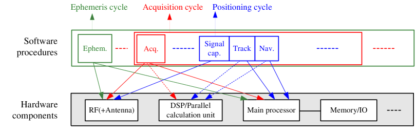
Figure 1: Architecture of a typical GPS receiver: main software procedures and associated hardware components. Dashed arrow lines mean possible association, depending on implementation.

Module/State	Power	Duration	Period
RF	$P_{r}$	$t_{r}$	$T$
Acquisition	$P_{a}$	$t_{a}$	$T_{a}$
Track	$P_{t}$	$t_{t}$	$T$
Ephemeris	$P_{e}$	$t_{e}$	$T_{e}$
Navigation	$P_{n}$	$t_{n}$	$T$
System Idle	$P_{i}$	$t_{i}$	$T$

Figure 2: Energy parameters of main software procedures and associated power levels.

We present an energy model that addresses the above challenges based on measurement with the Namuru V2 GPS receiver [4]. The model captures the architecture of a typical GPS receiver, as found in research-oriented [4] and industrial designs [21, 22, 5], while ignoring platform specific details and optimizations. The goal is not to predict absolute energy consumption of a general GPS module, but to shed light on the relationship between energy consumption and major software strategies. For the case of Namuru, a most notable finding is that the receiver’s energy consumption is roughly linear with the number of satellites to be tracked. Based on this finding, we propose a selective satellite tracking algorithm that minimally synchronizes with visible satellites, by taking advantage of the short term stability of satellite signal quality. Compared with the traditional full tracking algorithm, we obtain significant energy savings with negligible sacrifice on positioning accuracy. In summary, this paper makes two contributions:

• An energy model for GPS receivers showing the major energy consumers, and revealing the relationship between energy consumption and key software parameters. The model allows one to focus on the optimization of certain parts of GPS receiver software, which can be conveniently translated to energy gains. Being the first of its kind, the model provides a basis for our future investigation of a GPS receiver’s energy performance.

• A tracking algorithm that opportunistically avoids unnecessary satellite tracking for positioning. Real traces in two cities show that our new algorithm can save 20.9-23.1% energy consumption while retaining similar positioning accuracy.

2 GPS and GPS Receivers

The GPS navigation system is constituted of three components, satellites constellation, ground stations, and user receivers. The satellites constellation contains 32 satellites orbiting the Earth every 12 hours [7, 14]. The ground stations keep tracking the satellites’ health and trajectory configuration including the almanac and the ephemeris, which indicate the satellite’s status and precise location. All the satellites are precisely synchronized to atomic clocks within a few nanoseconds. Each satellite continuously broadcasts its time and trajectory message with CDMA signals at L1=1.575GHz (or L2=1.227GHz). GPS receivers capture raw GPS signals, decode the carrier/code information, and calculate their three-dimensional locations with a least square method.

Figure 2 shows the architecture of a typical GPS receiver design. From the perspective of software, the receiver mainly consists of five software procedures that are executed in cycles of different periods. In theory, the ephemeris data included in the satellite broadcast is only valid for 30 minutes, so the ephemeris data needs to be collected and decoded every 30 minutes. The acquisition procedure is executed every few minutes to extract the information of visible satellites. The positioning cycle refers to the time interval between two position updates to the application, and determines a system parameter known as update rate. Modern GPS modules often provide an update between 1 and 10 Hz. During each positioning cycle, the receiver calculates for a position, after which the receiver may enter a low-power sleep or idle state until the start of the next positioning cycle. Each positioning cycle involves three software procedures: signal capture and processing, (satellite) track, and navigation.

Each software procedure involves a number of hardware components. For example, the acquisition procedure is highly computation intensive and often requires dedicated hardware in addition to its use of the RF and the main processor. The main processor is in charge of task scheduling and general processing logic, so it is needed in all procedures. The specific hardware composition varies greatly across receiver manufacturers. For example, the SiRFstarIV chipset uses an ARM7 as the main processor and a DSP for faster signal processing [21], the ublox LEA-6 module [5] uses a dedicated hardware engine for massive parallel searches, while the Namuru receiver defines its CPU and parallel calculation unit with an Altera Cyclone 2C50 FPGA [4].

3 A Generic Energy Model

In this section we establish a generic energy model for a standard GPS receiver, assuming the architecture in Figure 2. Recall that we have identified five main procedures that dominate the energy consumption of a receiver: signal capturing and processing (i.e., the RF), acquisition, track, ephemeris extraction, and navigation. Some procedures span multiple positioning cycles (or simple cycles, when no confusion occurs), while others are on a per-cycle basis, all subject to a scheduler in the main processor. Given the typical single core configuration of the main processor, we can approximate the energy consumption of a procedure executed in scheduled time slots with its energy consumption during a complete and continuous run. A list of energy related variables is given in Figure 2.

Let $f$ be the update rate of the receiver, then the positioning cycle is $T=1/f$ seconds. The software procedures have the following energy characteristics:

• In each cycle, the RF captures raw GPS signal for a period of $t_{r}$ time, with a power level $P_{r}$. Normally, $1\sim 2$ms raw data suffices to produce a position [18], so $t_{r}=0.002$s.

• In the acquisition procedure, the receiver samples GPS signal for a period of $T_{r}$ time, and determines which satellites are in view by correlating the signal with a predefined C/A code, with an acquisition time $t_{a}$ and power $P_{a}$. For faster processing, the procedure may involve parallel computing units. In theory, the acquisition needs to be done only once for every period of ephemeris. However, in practice, the receiver may lose its lock with some of the satellites, so the actual operation of acquisition should be more frequent. In our experiments, an acquisition period of one minute turns out to work well, so we set $T_{a}=60$s.

• In the track procedure, the main processor calculates the precise Doppler frequency and code phase for each positioning cycle, with a track time $t_{t}$ and power $P_{t}$.

• In the ephemeris extraction procedure, the receiver has the RF continuously sample GPS signal for at least $t_{re}=36s$, and then the main processor calculates the status, position, and orbits of visible satellites, with a running time $t_{e}$ and power $P_{e}$, for every $T_{e}=30$ minutes. The calculation includes an acquisition and a track procedures.

• In the navigation procedure, the main processor calculates the receiver’s position by a least square method, with a running time $t_{n}$ and power $P_{n}$.

• The receiver enters an idle state and stays for $t_{i}$ time after obtaining a location fix in each cycle, with a power level $P_{i}$.

The total energy consumption of a GPS receiver in a time unit is:

$$P=P_{i}\frac{t_{i}}{T}+P_{r}\frac{t_{r}}{T}+\frac{P_{a}t_{a}+P_{r}t_{r}}{T_{a}}+P_{t}\frac{t_{t}}{T}$$ (1)

$$\quad+\frac{P_{e}t_{e}+P_{r}t_{re}}{T_{e}}+P_{n}\frac{t_{n}}{T}.$$

Transforming the power to the product of voltage and current gives:

$$P=U_{r}I_{r}\frac{t_{r}}{T}+\frac{U_{s}I_{a}t_{a}+U_{r}I_{r}t_{r}}{T_{a}}+U_{s}I_{t}\frac{t_{t}}{T}$$ (2)

$$\quad\quad+\frac{U_{s}I_{e}t_{e}+U_{r}I_{r}t_{re}}{T_{e}}+U_{s}I_{n}\frac{t_{n}}{T},$$

where $U_{r}$ and $I_{r}$ are the voltage and current of the RF module, $U_{s}$ the voltage of the main processor, and $I_{a}$, $I_{t}$, $I_{e}$, $I_{n}$ are the currents of the FPGA for the acquisition, track, ephemeris extraction and navigation procedures, respectively. These currents are different because the procedures may involve the main processor, parallel computing unit, and other memory system in different ways.

The system idle state is a deep power saving mode with $2\sim 3$ lower orders of magnitude than other modules, so it can be omitted. Plugging $T=1/f$ and the settings $t_{r}=0.002$, $T_{a}=60$, $t_{re}=60$, and $T_{e}=1800$ into Eq. 2, we have

$$P=0.002U_{r}I_{r}f+\frac{U_{s}I_{a}t_{a}+0.002U_{r}I_{r}}{60}+U_{s}I_{t}t_{t}f$$ (3)

$$\quad\quad+\frac{U_{s}I_{e}t_{e}+36U_{r}I_{r}}{1800}+U_{s}I_{n}t_{n}f.$$

4 The Case for Namuru Receiver

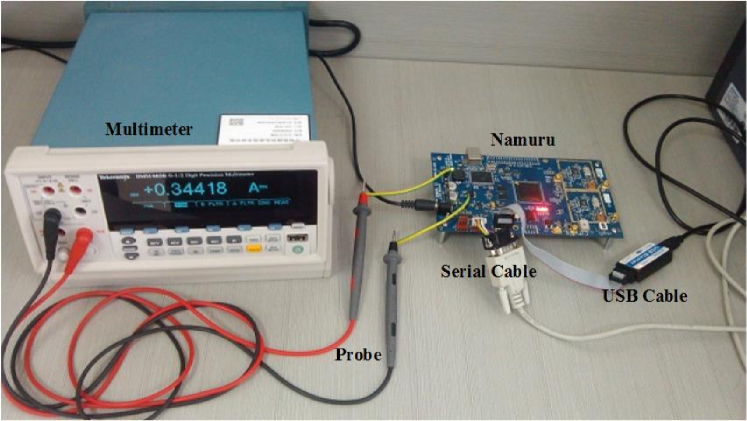
Figure 3: Energy parameter measurement system.

We study the energy model using the Namuru V2 receiver [4] as a concrete example. The goal is to determine the impact of key software parameters on energy efficiency. Two such parameters are considered: number of satellites to be tracked, denoted by $N$, and length of raw data (in milliseconds) to be sampled in each second, denoted by $L$. The more satellites to be synchronized, the higher positioning accuracy we get. The length of GPS data sampled per second determines the receiver’s maximum update rate which affects the resolution of position, since every position fix requires a certain length of raw data. In our setting, we use 2ms data for a position fix, therefore we have $L=2f$, in number.

The Namuru board is based on the Altera Cyclone 2C50 FPGA and contains a RF, RAMs/flashes, as well as IOs. We concentrate on core components such as the RF and FPGA. The measurement system is shown in Figure 3. The multimeter DMM4050 is connected to the Namuru board with its two probes, in order to record the realtime energy consumption of each module. To measure the voltage, the multimeter is connected to the RF or FPGA in parallel. To measure the current, a cascaded 0R resistance in the Namuru board is replaced by the multimeter probes.

To study the impact of individual software procedures on energy consumption, we reorganize the source code of the Namuru project, and create independent test units with configurable inputs of $N$ and $L$. These test units are created in the NIOS II IDE, downloaded to the FPGA, and then measured by the multimeter. Figure 4 (a) shows an example of the current measurement for three runs of the track procedure separated by intervals, after subtracting a constant baseline current of about 350 mA.

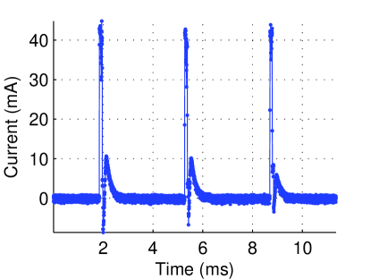
Figure 4: Current of the FPGA when running the track program for $L=2$ (after subtracting a constant baseline current).

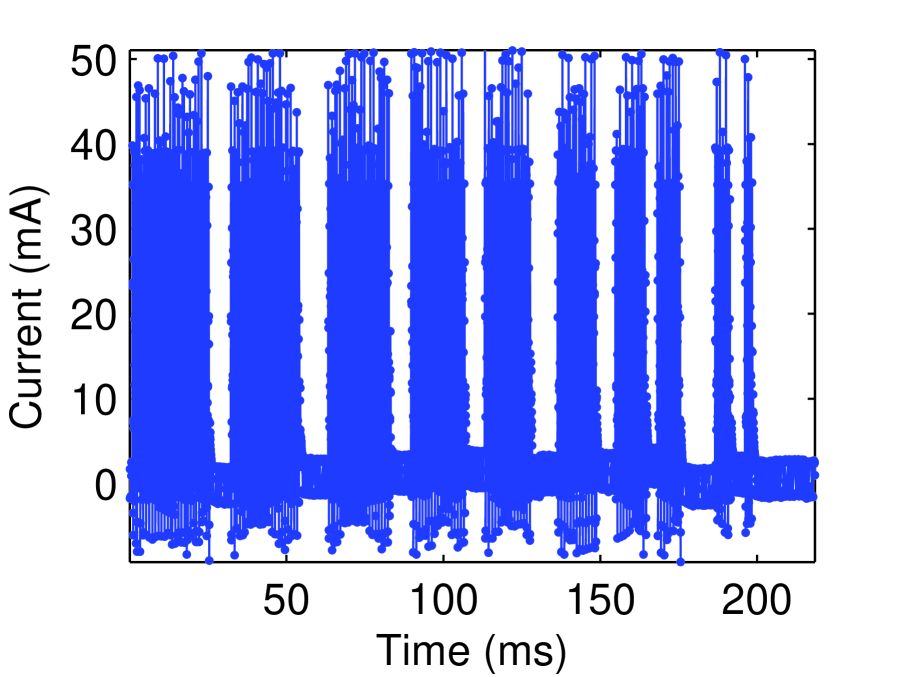
Figure 5: Current of FPGA running the track procedure for $N=10,9,\ldots,1$.

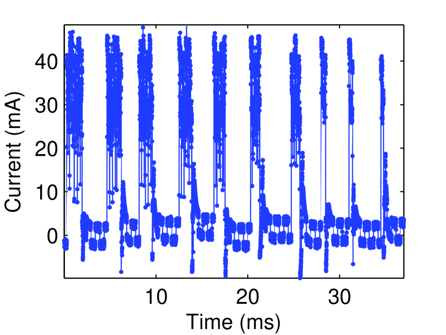
Figure 6: Current of FPGA running the navigation procedure for $N=10,9,\ldots,1$.

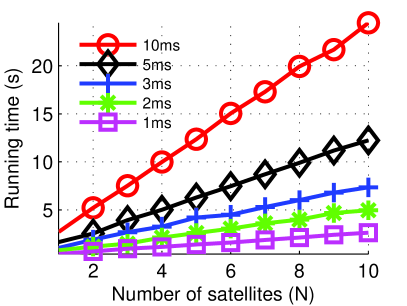
(a) Running time

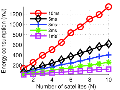
(b) Energy consumption

Figure 7: Running time and energy consumption of the track procedure vs. number of tracked satellites.

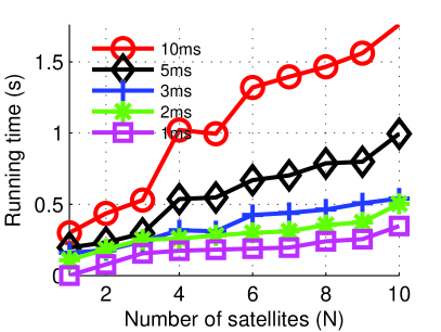
(a) Running time

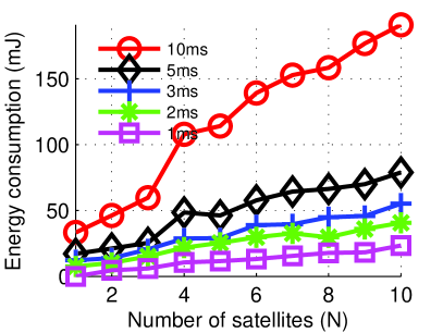
(b) Energy consumption

Figure 8: Running time and energy consumption of the navigation procedure vs. number of tracked satellites.

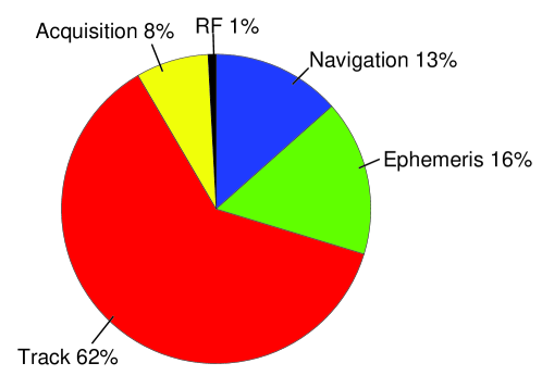
Figure 9: Average energy consumptions of different procedures.

RF. After removing the 0R resistance, the multimeter acquires the voltage $U_{r}=5$V and current $I_{r}=64$mA. Thus $P_{r}=0.002U_{r}I_{r}f=0.64fmW$. (There are two identical RF circuits and an additional frequency up-converter circuit on the Namuru board; we consider only the GPS L1 circuit.)

Acquisition. The acquisition procedure needs to search 30+ Doppler frequency bins and 8000+ code phases for each satellite, which is a very computation intensive operation. We disable the RF, import GPS signal traces manually, and run the acquisition test unit from a cold start. We obtain the voltage $U_{s}=3.3$V, the current $I_{a}=130$mA, and the running time $t_{a}=1.2$s. Considering the RF sampling procedure before each acquisition, the total energy consumption is $P_{a}=(U_{s}I_{a}t_{a}+0.002U_{r}I_{r})/60=8.59$ mW.

Track. A GPS receiver calculates the precise Doppler frequency and code phase in each positioning cycle. We measure the track current under different $N$ and $L$. Figure 6 shows the raw measurement of current under continuous tracking, for $L=10$ms and $N=10,9,\ldots,1$. In this figure, each continuous blue region represents a specific $N$. The current, multiplied by voltage, integrated over the duration of each such region measures the energy consumption of a procedure. Figure 7 shows how running time and energy consumption depend on $N$ and $L$. As can be seen, the energy consumption is roughly linear with $N$ and $L$, fitted with $P_{t}=11.88+7.26\cdot N\cdot L$ mW.

Ephemeris. We obtain $I_{e}=131$mA and $t_{e}=50$s in the cold start. with the addition of RF sampling, the whole energy consumption is $P_{e}=(U_{s}I_{e}t_{e}+36U_{r}I_{r})/1800=18.4$ mW.

Navigation. Similar to the track procedure, we measure the energy parameters under different $N$ and $L$. Figure 8 suggests that the energy consumption is roughly linear with $N$ and $L$, fitted with $P_{n}=2.0+1.65\cdot N\cdot L$ mW.

According to Eq. 3, the energy consumption for each positioning cycle are $P_{r}=0.64f$, $P_{a}=8.59$, $P_{t}=11.88+7.26NL$, $P_{e}=18.4$, $P_{n}=2.0+1.65NL$, in mW. So, the amortized energy consumption per second is as follows:

$$P=40.87+0.64\cdot f+8.91\cdot N\cdot L$$ (4)

$$\quad=40.87+0.64\cdot f+17.82\cdot N\cdot f.$$

Figure 9 presents a breakdown of the different procedures’s energy consumption on Namuru with $N=8$ satellites tracked and $f=1$Hz location update rate. It can be seen that the dominant energy consumer is the track procedure, expending up to 62% of the total energy. This is partly because this procedure is in the innermost loop of the processing flow (Figure 2), and partly because it involves intensive computation itself.

5 Energy Efficient Tracking

The model in eq. 4 suggests that if one manage to reduce the number of tracked satellites or update rate, then the energy consumption can be reduced considerably. The problem is how to retain the positioning accuracy at the same time. We make an initial investigation in this section, considering the parameter $N$, with $f=1$.

5.1 Selective Tracking

Traditional track algorithms attempt to track all visible satellites as indicated by the ephemeris information, and then use all or part of the satellites to calculate positions. Our approach is to track only a subset of the visible satellites that are just enough to produce equally accurate positions. The observation behind is that the signal quality of satellites remains stable for at least a short period of time (e.g., minutes), and that the contributions of available satellites to position quality are nonuniform. Thus, we can perform full tracking only sparingly, and selectively track a subset of satellites whose collective quality is close to that of the full set.

Satellite weight. The geometric dilution of precision (GDOP) is a scaling factor to show the pseudorange error between the receiver and available satellites, which can be determined as follows:

$$\mbox{GDOP}=\sqrt{\mbox{trace}(A^{T}A)^{-1}},$$ (5)

$$A=\begin{bmatrix}u_{1}&v_{1}&w_{1}&1\\ u_{2}&v_{2}&w_{2}&1\\ \vdots&\vdots&\vdots&1\\ u_{r}&v_{r}&w_{r}&1\\ \end{bmatrix},$$

where $A$ is a geometry matrix between the receiver and available satellites, ($u_{i},v_{i},w_{i})$ is the normalized direction vector between the receiver and the $i^{th}$ satellite, and $r$ is the number of available satellites.

Suppose $W$ is a weight matrix to indicate each satellite’s contribution to minimize the GDOP, which equals to minimize the convariance matrix $(A^{T}WA)^{-1}$ [19].

With $M=A(A^{T}WA)^{-1}$, it can be proved that

$$\begin{split}\mbox{trace}(A^{T}WA)^{-1}=\mbox{trace}(WMM^{T})\\ =\sum_{i=1}^{r}\sum_{j=1}^{4}w_{ii}m_{ij}^{2}\triangleq f(W).\end{split}$$ (6)

Then, differentiate $f(W)$ to minimize $f(W)$ as follows:

$$\frac{\partial f(W_{kk})}{\partial w_{kk}}=\sum_{j=1}^{4}m_{kj}^{2}=0,$$ (7)

which can be solved with an iteration method to derive $W_{kk}$.

Satellite selection. In selective tracking, satellites are selected as follows. Suppose the current satellite set $S$ has a total GDOP $G$. First, calculate each satellite’s contribution to the positioning accuracy with the above satellite weight algorithm. Then, choose a satellites subset $S_{w}$ with three largest weights, and obtain its GDOP, denoted by $G_{w}$. This subset is considered qualified if $\left|G-G_{w}\right|/G<5\%$. Otherwise, add the largest weight satellite in subset $S-S_{w}$ to $S_{w}$, until $\left|G-G_{w}\right|/G<5\%$. Note that traditional positioning algorithm requires at least four satellites to determine the receiver’s location. With the historical receiver’s location, the altitude is known and so three satellites are sufficient for positioning.

We have found that the relative GDOPs of satellites usually remain stable during intervals of minutes, though their absolute values vary over time. Thus, the satellite selection algorithm (following a full tracking operation) only needs to be performed every few minutes. In our setting, it is executed once a minute. The computation involves simple operations on small-sized matrices ($r\times 4$ in our case), a small number of iterations for minimizing $f(W)$ (normally 3, with dynamic adjustment of search step size), and a greedy selection algorithm, so the per-second overhead, in terms of both computation load and energy consumption, is negligible.

5.2 Evaluation

Experimental setup. We evaluate our algorithm using real mobile data traces. Two GPS samplers were used, HG-SOFTGPS02 [3] and Namuru [4], shown in Figures 10(a) and (b). These GPS samplers collect 2bit data, with a sampling frequency 16.368 MHz and an intermediate frequency 4.092 MHz.

While sampling the data on the vehicle, we used a professional handheld GIS data collector S750 to obtain the ground truth of positions [2]. As shown in Figure 10(c), the collector has a professional GPS module with post-processed kinematic mode and CORS network access authority. It provides an update rate of 1 Hz with sub-meter accuracy. We collected two traces. The first trace is about 4.8 km long, obtained on a highway with 60 km/h velocity. The full tracking method finds 6-8 effective satellites on this road, and generates 11.8m location accuracy. The other traces was gathered from a different city which is 2,000 km away. In this scenario, our vehicle traveled along a 4 km curved road with many viaducts. The full tracking method has 13.1m location accuracy with 5-7 satellites in sight.

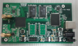
(a)

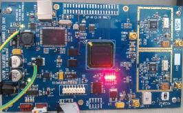
(b)

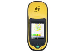
(c)

Figure 10: GPS samplers and a professional positioning device for obtaining ground truth. (a) HG-SOFTGPS02 sampler. (b) Namuru. (c) Handheld GIS data collector S750.

Evaluation results. We compare the receiver’s position under selective tracking (ST) and under full tracking (FT) on these two traces. Figure 11 presents the calculated trajectories of the vehicles under ST (red line), FT (blue line), in comparison with the ground truth (green line). For the first trace, FT produces a mean position accuracy of 11.9m. ST generates a mean position accuracy 12.7m, with a 23.1% energy saving. For the second trace, FT generates 13.1m location accuracy, while ST shows accuracy of 13.4m, with a 20.9% energy saving.

We also consider a random tracking (RT) method, in which a certain number of satellites are randomly chosen for tracking. Figure 12 demonstrates the positioning accuracy of the three tracking methods. For the maximum number of randomly chosen satellites 6, 5, 4, RT provides position accuracy of 20.9m, 23.2m, and 51.2m, respectively.

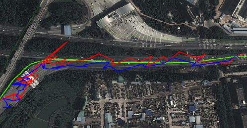
(a) Trace one.

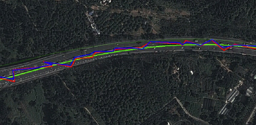
(b) Trace two.

Figure 11: The moving trajectories of the GPS receiver under ST (red line), FT (blue line), and ground truth (green line).

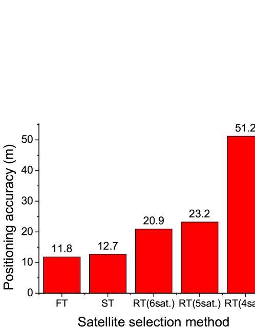
Figure 12: Positioning accuracy of full tracking (FT), selective tracking (ST) and random tracking (RT) with different numbers of satellites.

6 Related work

Low power location sensing. EnLoc [9] computes optimal locations with off-line dynamic programming, and then selects a localization technology from GPS, WiFi and GSM for a given energy budge. EnTracked [15] adjusts the GPS sampling rate based on the estimation and prediction of system conditions and mobility. RAPS [23] presents a rate-adaptive positioning system based on velocity estimation from historical GPS readings. It also estimates user movement with a duty-cycled accelerometer, and utilizes Bluetooth communication with neighboring devices to reduce position uncertainty. A-Loc [17] builds accuracy models and energy models for various location sensors, and then designs an algorithm to determine the most energy efficient sensor for mobile applications. SensLoc [16] designs a place detection algorithm to find contextual information (e.g., home, office) from sensor signals, and then controls the active duty cycle of a GPS receiver and other sensors. SmartLoc [6] is a localization system to estimate the location and traveling distance with low power inertial sensors.

In general, these techniques are less power consuming than using GPS alone, but can be much less accurate in positioning.

Computation optimization. The signal acquisition process usually consists of a two-dimension Fourier transform, which has a complexity of $O(n\log n)$ for Fast Fourier Transform (FFT), where $n$ is the number of signal samples. Hassanieh [10] presents a sparse Fourier Transform to reduce the complexity from $O(n\log n)$ to $O(n\sqrt{\log n})$. While the practical improvement is significant, sparse Fourier transform based method only simplifies the acquisition progress, and makes very limited contribution to the whole energy consumption of GPS positioning. Liu et al. [18, 20] propose to offload the computation intensive tasks into a cloud server. For each location fix, the GPS receiver only has to collect and store milliseconds raw GPS signal. This approach is limited to off-line positioning applications.

7 Discussion and Conclusion

Although our abstract model in Eq. 3 provides an framework to capture the major software components of a general GPS receiver, instantiating the model for a specific receiver still requires the knowledge of the receiver’s hardware structure, and means to measure the power of individual hardware units. This is not possible for closed and proprietary GPS receivers such as those found in today’s commercial phones. In that case, one can perform black-box testing to show the impact of certain system parameters (e.g., update rate) on energy consumption, but the obtainable information is likely to be very restricted – for example, it is not possible to obtain the power breakdown of the different software/hardware components, which makes it hard to identify the major energy consumers. As such, our model with Namuru is only the first step toward a complete understanding of this important module on mobile devices.

Based on the energy model, we have studied only a simple optimization to a single system parameter $N$. In the future, we will consider jointly optimizing multiple procedures and parameters, and exploiting other location sensors to achieve improved tradeoffs between positioning accuracy, energy consumption, and solution applicability.

References

-
[1]
Error analysis for the Global Positioning System.
http://en.wikipedia.org/wiki/Error_analysis_for_the_Global_Positioning_System. -
[2]
Handheld GIS Data Collector S750.
http://en.southinstrument.com/products/pro_info.asp?id=334. -
[3]
HG-SOFTGPS02.
http://www.hellognss.com/English/. -
[4]
Namuru GPS receiver.
http://www.dynamics.co.nz/index.php?main_page=page&id=11. - [5] U-blox Inc. LEA-6 u-blox 6 GPS Modules Data Sheet. http://www.u-blox.com.
- [6] C. Bo, X. Li, T. Jung, X. Mao, Y. Tao, and L. Yao. SmartLoc: Push the Limit of the Inertial Sensor Based Metropolitan Localization Using Smartphone. In MobiCom, 2013.
- [7] K. Borre, D. Akos, N. Bertelsen, P. Rinder, and S. Jensen. A Software-Defined GPS and Galileo Receiver A Single-Frequency Approach. Birkhauser Engineering, 2007.
- [8] A. Carroll and G. Heiser. An Analysis of Power Consumption in a Smartphone. Proc. of the 2010 USENIX Annual Technical Conference.
- [9] I. Constandache, S. Gaonkar, M. Sayler, R. Choudhury, and L. Cox. EnLoc: Energy-Efficient Localization for Mobile Phones. In INFOCOM, 2009.
- [10] H. Hassanieh, F. Adib, D. Katabi, and P. Indyk. Faster GPS via the Sparse Fourier Transform. In MobiCom, 2012.
- [11] W. Hedgecock, M. Maroti, J. Sallai, P. Volgyesi, and A. Ledeczi. High-Accuracy Differential Tracking of Low-Cost GPS Receivers. In MobiSys, 2013.
- [12] R. Jurdak, P. Corke, D. Dharman, and G. Salagnac. Adaptive GPS Duty Cycling and Radio Ranging for Energy-efficient Localization. In SenSys, 2010.
- [13] R. Jurdak, P. Corke, D. Dharman, and G. Salagnac. Energy-efficient Localisation: GPS Duty Cycling with Radio Ranging. In ACM Transactions on Sensor Networks, 9(3), 2013.
- [14] E. Kaplan and C. Hegarty. Understanding GPS Principles and Applications, Second Edition. Artech House, 2005.
- [15] M. Kjaergaard, J. Langdala, T. Godsk, and T. Toftkjaer. EnTracked: Energy-Efficient Robust Position Tracking for Mobile Devices. In MobiSys, 2009.
- [16] D. Lim, Y. Kim, D. Estrin, and M. Srivastava. SensLoc: Sensing Everyday Places and Paths using Less Energy. In Sensys, 2010.
- [17] K. Lin, L. Jolla, A. Kansal, D. Lymberopoulos, and F. Zhao. Energy-Accuracy Trade-off for Continuous Mobile Device Location. In MobiSys, 2010.
- [18] J. Liu, B. Priyantha, T. Hart, H. Ramos, A. Loureiro, and Q. Wang. Energy Efficient GPS Sensing with Cloud Offloading. In SenSys, 2012.
- [19] E. Mok and P. A. Cross. A Fast Satellite Selection Algorithm for Combined GPS and GLONASS Receivers. Journal of Navigation, 47(3),1994,383-389.
- [20] H. Ramos, T. Zhang, J. Liu, N. Priyantha, and A. Kansal. LEAP: A Low Energy Assisted GPS for Trajectory-Based Services. In UbiComp, 2011.
- [21] SiRF Technology, Inc. SiRFstarIV GSD4e: High-sensitivity GPS Location Processor with Built-in CPU and SiRFaware Technology. April 2010, Issue 2, Part Number CS-130621-PB.
- [22] SiRF Technology, Inc. Control and Features for Satellite Positioning System Receivers. December 2011, Part Number US2011/0316741-A1.
- [23] J. Paek, J. Kim, and R. Govindan. Energy-Efficient Rate-Adaptive GPS-based Positioning for Smartphones. In MobiSys, 2010.
- [24] Z. Zhuang, K. Kim, and J. Singh. Improving Energy Efficiency of Location Sensing on Smartphones. In MobiSys, 2010.