Far beyond stacking: Fully bayesian constraints on sub-microJy radio source populations over the XMM-LSS–VIDEO field

Abstract

Measuring radio source counts is critical for characterizing new extragalactic populations, brings a wealth of science within reach and will inform forecasts for SKA and its pathfinders. Yet there is currently great debate (and few measurements) about the behaviour of the 1.4-GHz counts in the $\mu$Jy regime. One way to push the counts to these levels is via ‘stacking’, the covariance of a map with a catalogue at higher resolution and (often) a different wavelength. For the first time, we cast stacking in a fully bayesian framework, applying it to (i) the SKADS simulation and (ii) VLA data stacked at the positions of sources from the VIDEO survey. In the former case, the algorithm recovers the counts correctly when applied to the catalogue, but is biased high when confusion comes into play. This needs to be accounted for in the analysis of data from any relatively-low-resolution SKA pathfinders. For the latter case, the observed radio source counts remain flat below the 5-$\sigma$ level of 85 $\mu$Jy as far as 40 $\mu$Jy, then fall off earlier than the flux hinted at by the SKADS simulations and a recent $P(D)$ analysis (which is the only other measurement from the literature at these flux-density levels, itself extrapolated in frequency). Division into galaxy type via spectral-energy distribution reveals that normal spiral galaxies dominate the counts at these fluxes.

1 Introduction

Measurements of radio source counts provided some of the earliest cosmological support for an expanding Universe, but today they can be used to discover and characterize new extragalactic populations (see e.g. Massardi et al. 2011; Mahony et al. 2011; Whittam et al. 2013; Franzen et al. 2014) and/or to shed light on galaxy evolution in allowing (together with redshift information) inference of star-formation rates and luminosity functions (see e.g. Dunne et al. 2009; Karim et al. 2011; Roseboom and Best 2014; Zwart et al. 2014a). It is also critical to pin them down in advance of the new wave of radio telescopes such as MeerKAT, ASKAP and SKA1: since confusion noise (Scheuer 1957; Condon 1974, 1992; Condon et al. 2002, 2012) depends directly on the source counts and a telescope’s synthesized beam, the level of confusion noise is both a function of these two and informs the desired telescope configuration. It is therefore essential to measure counts for both telescope design and survey forecasting for SKA and its pathfinders (see e.g. Zwart et al. 2014b). See also de Zotti et al. (2010) for a review of the counts at a range of radio frequencies.

There is currently considerable debate about the behaviour of 1.4-GHz differential source counts at $\lesssim\mu$Jy levels, ARCADE2 (Seiffert et al., 2011; Fixsen et al., 2011) finding them to be relatively flat (in the Euclidean normalization, i.e. flux density $S^{2.5}$) below 100$\mu$Jy, but with VLA 3-GHz measurements by Condon et al. (2012) hinting that they are rather steeper (roughly $\propto S^{-1.5}$ from that work) at those flux-density levels. The work of Owen and Morrison (2008) showed the need for careful corrections for source angular diameters when assembling 1.4-GHz source counts. Heywood et al. (2013) suggested the considerable variation in the source counts at 100$\mu$Jy could be attributed to sample variance. Indeed, a more-detailed analysis (see below) of the Condon et al. data by Vernstrom et al. (2014) confirmed the steep counts down to sub-$\mu$Jy levels; their result is still compatible with the Seiffert et al. data only with a new, somewhat extreme population of very faint sources. Finally, the state-of-the-art SKADS simulations (Wilman et al., 2008) also require the source counts to be steep (and steepening) at the $\mu$Jy level. With all this in mind, there is a clear need for more and complementary measurements in this area, especially in the run up to SKA1 and as its pathfinders come online.

Three main methods exist for determining source counts. In the first, traditionally astronomers simply counted directly-detected sources in flux bins above some well-motivated threshold (usually $5\times$ the rms noise for the radio-source catalogue, but e.g. AMI Consortium et al. 2011b even used $4.62\times$ rms).

Second, Scheuer (1957) showed that faint, unresolved sources buried within the thermal noise could contribute a variance term from their (positive) flux as well as from their (negative) synthesized-beam sidelobes. Hence (see also above) measuring the noise allows one to constrain source counts (a so-called probability of deflection, or $P(D)$, analysis) if the confusion contribution is dominant. Hewish (1961) was the first to use Scheuer’s blind method, and it was most recently implemented (in the image plane) at 3 GHz by Condon et al. (2012) and Vernstrom et al. (2014), then extrapolated to 1.4 GHz.

The third approach is ‘stacking’. One would like to push source-count measurements as deep as possible, but a $P(D)$ analysis is not possible unless a radio map is confusion-noise-limited. However, if one knew in advance the positions of sources below the formal detection threshold, for example from some deeper auxiliary catalogue, one could constrain source counts below the detection threshold using this prior information and accounting for that thermal noise. Such a selection effect is a both a blessing and a curse: stacking allows for a robust ‘source-frame’ definition and subsequent subdivision of the sample, but cannot ever capture properties of a population defined by an ‘observer-frame’ blind analysis such as $P(D)$. The method has been applied in a number of different settings, e.g. in polarization (Stil et al., 2014), in the sub-mm (Patanchon et al., 2009) and at 1.4 GHz (Seymour et al., 2008; Hales et al., 2014a, b).

Marsden et al. (2009) formally define stacking as taking the covariance of a map with a catalogue (at any two wavebands), but in fact it has many flavours in the literature as pointed out by Zwart et al. (2014a). In the past (Dunne et al., 2009; Karim et al., 2011; Zwart et al., 2014a) some single statistic (usually an average such as the mean or median) has been used to summarize the properties of radio pixels stacked at the positions from the auxiliary catalogue, allowing calculation of, for example, star-formation rates in mass-redshift bins. The precision on any inferred parameters scales as $N_{\mathrm{sources}}^{-1/2}$ (Roseboom and Best, 2014), so for (say) 40,000 sources a statistical factor of 200 in sensitivity below the survey threshold could in theory be achieved.

However, the data afford more information than what is encoded in a single summary statistic (and careful attention must be paid to potential biases in those analyses; see Zwart et al. 2014b). For example, Bourne et al. (2012) identify three potential sources of bias in median stacking: the flux limits and shape of the ‘true’ underlying flux distribution, and the amplitude of the thermal noise. Rather than being viewed as biases, such extra information in the observed data can be exploited in order to infer the parameters of some underlying physical model.

This was demonstrated by Mitchell-Wynne et al. (2014) who constrained 1.4-GHz source counts down to $\sigma/10$ from FIRST maps (Becker et al., 1995) stacked, at positions from deeper COSMOS data (Scoville et al., 2007), by fitting a power-law model to the noisy map-extracted flux distribution. Using a similar parametric method, Roseboom and Best (2014) included redshift information in order to measure the evolution of the 1.4-GHz luminosity function for near-infrared-selected galaxies, which they called ‘parametric stack-fitting’.

In this work we extend the algorithm of Mitchell-Wynne et al. (2014) in the following ways: (i) We cast the problem in a fully bayesian framework rather than in a purely maximum-likelihood one; (ii) in our framework we consider the use of the bayesian evidence for selecting between different source-count models; we demonstrate the algorithm on the SKADS simulations; and (iv) we apply the algorithm to a deep ($K_{\mathrm{s}}\,<23.5$) mass-selected data sample from the VIDEO survey (Jarvis et al., 2013).

In section 2 we describe our bayesian framework, including the models, priors and likelihoods we use. We give some details of simulations undertaken in section 3, with a description of the near-infrared and radio observations and data in section 4. We present our results and discussion in section 5 before concluding in section 6.

We assume radio spectral indices $\alpha$ are such that $S_{\nu}\propto\nu^{\alpha}$ for a source of flux density $S_{\nu}$ at frequency $\nu$. All coordinates are epoch J2000. Magnitudes are in the AB system. We assume a $\Lambda$CDM ‘concordance’ cosmology throughout, with $\Omega_{\mathrm{m}}=0.3$, $\Omega_{\Lambda}=0.7$ and $H_{0}=70\,\mathrm{km\,s^{-1}}\,\mathrm{Mpc}^{-1}$ (Komatsu et al., 2011).

2 Bayesian Framework

2.1 Bayes’ Theorem

Bayesian analyses of astronomical data sets have become commonplace in the last ten years (see e.g. Feroz et al. 2009b, Feroz et al. 2011, Zwart et al. 2011, Lochner et al. 2015) because of their many advantages. The targeted posterior probability distribution $\mathcal{P}\left(\mathbf{\Theta}|\mathrm{\mathbf{D}},H\right)$ of the values of the parameters $\mathbf{\Theta}$, given the available data $\mathrm{\mathbf{D}}$ and a model $H$ (the model is a hypothesis plus any assumptions), comes from Bayes’ theorem:

$$\mathcal{P}\left(\mathbf{\Theta}|\mathrm{\mathbf{D}},H\right)=\frac{\mathcal{L}\left(\mathrm{\mathbf{D}}|\mathbf{\Theta},H\right)\mathit{\Pi}\left(\mathbf{\Theta}|H\right)}{\mathcal{Z}\left(\mathrm{\mathbf{D}}|H\right)}.$$ (1)

In the numerator, the likelihood $\mathcal{L}\left(\mathrm{\mathbf{D}}|\mathbf{\Theta},H\right)$, i.e. the probability distribution of the data given parameter values and a model, encapsulates the experimental constraints. The prior $\mathit{\Pi}\left(\mathbf{\Theta}|H\right)$ records prior knowledge of or prejudices about the values of the parameters. The bayesian evidence, $\mathcal{Z}\left(\mathrm{\mathbf{D}}|H\right)$, is the integral of $\mathcal{L}\left(\mathrm{\mathbf{D}}|\mathbf{\Theta},H\right)\mathit{\Pi}\left(\mathbf{\Theta}|H\right)$ over all $\mathbf{\Theta}$. Naïvely it normalizes the posterior in parameter space; crucially it facilitates selection between different models when their evidences are compared quantitatively (Occam’s razor; see e.g. MacKay 2003).

2.2 Sampling

Carrying out the evidence integrations and sampling the parameter space has not in the past been easy and was often slow. Nested sampling (Skilling, 2004) was invented specifically to reduce the computational cost of evidence calculations, since no posterior sample (each of which is obtained ‘for free’) is ever wasted. However, the integrations are exponential in the number of model parameters, typically limiting that number to O($10^{2}$) on current machines. A particularly robust and efficient implementation of nested sampling is MultiNest (Feroz and Hobson, 2008; Feroz et al., 2009a; Buchner et al., 2014), which permits sampling from posteriors that are multimodal and/or unusually shaped. Posterior distributions are represented by full distributions rather than a summary mean/median value and a (perhaps covariant) uncertainty, since this represents the total inference about the problem at hand, and error propagation is fully automatic.

In what follows we used a python interface (Buchner et al., 2014) to MultiNest, deployed in parallel on (typically) 96 processors. Because of the unusually-shaped posterior distributions, there were often as many as O(100,000) likelihood evaluations. However, the resources required for the algorithm are not heavy on either memory or disk space: it is the number of parallel processors that controls the (rejection) sampling efficiency and hence total wall execution time.

2.3 Models considered here

We treat four source-count models here, each encoding some functional form with a number of parameters and incorporating priors on each of those parameters, plus any assumptions. The evidence will be employed to select between several piecewise-linearly-interpolated power-law models (A, B, C and D) by way of example, but any parametric model could be used be it a modified power law, a polynomial or a pole/node-based model (see e.g. Bridges et al. 2009, Vernstrom et al. 2014).

2.3.1 Model A

For the single-power law, we have simply that

$$\frac{\mathrm{d}N}{\mathrm{d}S}\left(C,\alpha,S_{min},S_{max}\right)=\begin{cases}CS^{\alpha}&S_{min}<S<S_{max}\\ 0&\mathrm{otherwise}\\ \end{cases},$$ (2)

where $\frac{\mathrm{d}N}{\mathrm{d}S}$ is the differential count for $N$ sources in the flux interval $\left[S,S+\mathrm{d}S\right]$ ($\mathrm{Jy}$). $C$ is a normalization constant ($\mathrm{sr}^{-1}\mathrm{Jy}^{-1}$), $\alpha$ is a slope, and the model is set to zero outside the lower and upper limits $S_{min}$ and $S_{max}$. We denote the parameter vector $\mathbf{\Theta_{A}}=\{C,\alpha,S_{\mathrm{min}},S_{\mathrm{max}}\}$.

2.3.2 Models B, C and D

Model B extends Model A with a second power law (two extra parameters), i.e. it incorporates a second slope $\beta$ with a break at $S_{0}$ ($S_{min}<S_{0}<S_{max}$):

$$\frac{\mathrm{d}N}{\mathrm{d}S}\left(C,\alpha,\beta,S_{0},S_{min},S_{max}\right)\\ =\begin{cases}CS^{\alpha}&S_{min}<S<S_{0}\\ C\,S_{0}^{\alpha-\beta\,}S^{\beta}&S_{0}<S<S_{max}\\ 0&\mathrm{otherwise}\\ \end{cases},$$ (3)

with a parameter vector $\mathbf{\Theta_{B}}=\{C,\alpha,\beta,S_{0},S_{\mathrm{min}},S_{\mathrm{max}}\}$. Model C incorporates another break in the power law, so $\mathbf{\Theta_{C}}=\{C,\alpha,\beta,\gamma,S_{0},S_{1},S_{\mathrm{min}},S_{\mathrm{max}}\}$, and Model D, a third break, i.e. $\mathbf{\Theta_{D}}=\{C,\alpha,\beta,\gamma,\delta,S_{0},S_{1},S_{2},S_{\mathrm{min}},S_{\mathrm{max}}\}$. Priors on the different model parameters are discussed in section 2.4.

2.3.3 Models A′, B′, C′ and D′

In section 5 we investigate some scenarios where we allow the flux-measurement noise $\sigma_{n}$ (see section 2.5) to be a free parameter of the fit. We denote these models A′, B′, C′ and D′ corresponding to their fixed-noise counterparts A, B, C and D respectively.

2.4 Priors

It is straightforward to vary the priors $\mathit{\Pi}\left(\mathbf{\Theta}|H\right)$ on parameters $\mathbf{\Theta}$; the ones we adopt are shown in Table 1. In particular the power-law normalization $C$, as a scale parameter, is given a logarithmic prior, and any power-law breaks are free to vary their positions.

We assume all model hypotheses to be equally likely ab initio, which is equivalent to considering solely the Bayes factor $\mathcal{Z}_{1}\left(\mathrm{\mathbf{D}}|H_{1}\right)/\mathcal{Z}_{2}\left(\mathrm{\mathbf{D}}|H_{2}\right)$ when comparing models.

Table 1: Priors $\mathit{\Pi}\left(\mathbf{\Theta}|H\right)$ adopted here.

Parameter	Prior
$C/\mathrm{sr^{-1}Jy^{-1}}$	log-uniform $\in\left[10^{-5},10^{7}\right]$
$\alpha,\beta,\gamma,\delta$	uniform $\in\left[-2.5,-0.1\right]$
$S_{min}/\mu$Jy	uniform $\in\left[0.01,20.0\right]$
$S_{max}/\mu$Jy	uniform $\in\left[20.0,100.0\right]$
$S_{0,1,2}$	uniform $\in\left[S_{min},S_{max}\right]$
$S_{0,1,2}$	further require $S_{0}<S_{1}<S_{2}$
$\sigma_{n}$	$\delta\left(\sigma_{\mathrm{survey}}\right)$, or
	uniform $\in\left[0.5,2.0\right]\sigma_{\mathrm{survey}}$

2.5 Likelihood Function

In what follows we drop an explicit dependence on $\mathcal{H}$ but do note our assumptions along the way. We cannot use a simple gaussian ($\chi^{2}$) likelihood function because the measurement uncertainties are not themselves gaussian: since we are dealing with binned data we adopt a poisson likelihood. For the $i^{th}$ bin containing $k_{i}$ objects, the corresponding likelihood $\mathcal{L}_{i}\left(k_{i}|\boldsymbol{\theta}\right)$ is

$$\mathcal{L}_{i}\left(k_{i}|\boldsymbol{\theta}\right)=\frac{I_{i}^{k_{i}}\mathrm{e}^{-I_{i}}}{k_{i}!},$$ (4)

where

$$I_{i}=\int_{S_{min}}^{S_{max}}\mathrm{d}S\frac{\mathrm{d}N(S)}{\mathrm{d}S}\int_{S_{m_{i}}}^{S_{m_{i}}+\Delta S_{m_{i}}}\mathrm{d}S_{m}\frac{1}{\sigma_{n}\sqrt{2\pi}}\mathrm{e}^{-\frac{\left(S-S_{m}\right)^{2}}{2\sigma_{n}^{2}}}.$$ (5)

The second integral accounts for the gaussian map noise. $I_{i}$ is, in a sense, a mock realisation of the count in a particular bin from a specific set of parameter values, to be compared with the real values encoded by $k$. Folded into $I_{i}$ are the flux-measurement noise $\sigma_{n}$ (assumed here to be the same for all objects, i.e. constant across the field, $\sigma_{j}=\sigma_{n}\forall j$ sources) and the bin limits $\left[S_{m_{i}},S_{m_{i}}+\Delta S_{m_{i}}\right]$. $S$ and $S_{m}$ are respectively the measured and noise-free fluxes for the sources in a given bin, related by $S\sim\mathcal{N}\left(S_{m},\sigma_{n}^{2}\right)$. Carrying out the second integration in equation 5 gives

$$I_{i}=\int_{S_{min}}^{S_{max}}\mathrm{d}S\frac{\mathrm{d}N(S)}{\mathrm{d}S}\\ \frac{1}{2}\left\{\mathrm{erf}\left(\frac{S-S_{m_{i}}}{\sigma_{n}\sqrt{2}}\right)-\mathrm{erf}\left(\frac{S-(S_{m_{i}}+\Delta S_{m_{i}})}{\sigma_{n}\sqrt{2}}\right)\right\}.$$ (6)

Assuming independent bin entries, the likelihoods multiply (the log-likelihoods adding) to give the total likelihood for the $n_{bins}$ bins:

$$\mathcal{L}\left(\mathbf{k}|\boldsymbol{\theta}\right)=\prod_{i=1}^{n_{bins}}\mathcal{L}_{i}\left(k_{i}|\boldsymbol{\theta}\right).$$ (7)

When combined with the priors from Table 1, inserting equation 7 into equation 1 yields the posterior probability distribution (for parameter estimation) and the bayesian evidence (for model selection).

As a final point, it is possible to jointly infer an assumed-constant measurement noise, including any contribution from confusion noise, at the same time as the source-count model parameters. Hence the source-count model could simultaneously be extended to even fainter fluxes, as well as to the inclusion of brighter sources above the detection threshold.

With the formalism for the priors and likelihoods in place, we have all of the ingredients we need to calculate posterior probability distributions and the evidences for each model. We now turn our attention to testing the algorithm on simulations.

3 Simulations

The Square Kilometre Array Design Studies SKA Simulated Skies (SKADS–S³) simulation (Wilman et al., 2008, 2010) is a semi-empirical model of the extragalactic radio-continuum sky covering an area of 400 deg², from which we extracted a 1-deg² catalogue at 1.4 GHz for the purposes of testing our method. The simulation, which is the most recent available, incorporates both large- and small-scale clustering and has a flux limit of 10 nJy. We undertook several tests as follows.

First, we took all $\approx$ 375,000 of the noise-free 1.4-GHz fluxes ($<85\mu$Jy, i.e. the 5-$\sigma$ limit of our radio map — see section 4.2) and added gaussian random noise of standard deviation equal to the modal VLA map 1-$\sigma$ noise (i.e. 16.2 $\mu$Jy). We divided the resulting mock catalogue into 38 bins, $-68<S/\mu$Jy $<85$, with the lower edge of the lowest bin being the flux of the faintest source in the noisy catalogue. Fitting each of models A, B, C and D in turn, we found that model B (one break) returned the highest evidence (Table 2). Figure 1 is the posterior probability distribution of the parameters for that model.

A bayesian framework allows us to explore the full posterior, rather than simply determining the position of its peak, even though the distribution is highly non-gaussian. For example, there is a strong degeneracy between $C$ and $\alpha$; there is a hard diagonal edge in the positions of adjacent power-law breaks because of the constraint that e.g. $S_{0}<S_{1}<S_{2}$; alternate power laws tend to be anti-correlated in their parameters; and overall there is little symmetry in the posterior. A fully bayesian analysis such as ours is essential because so many of the assumptions of a maximum-likelihood approach have broken down. The bayesian evidence is in turn the appropriate tool to be used for model selection in place of a $\Delta\chi^{2}$ — an estimator that would not have told the whole story.

We have deliberately not tabulated maximum a posteriori (MAP), maximum-likelihood or ‘best-fit’ parameter values because even the 1-D marginalized posteriors are misleading in their masking of the intricate characteristics of the full posterior probability distribution. Point estimates such as the maximum-likelihood and MAP are subject to noise and hence are not very representative of the full posterior. Rather, we reconstruct source counts directly from the ensemble of posterior samples, as follows. Figure 2 shows the source-count reconstruction based on (the winning) model B. For each sample from the posterior, we have generated a corresponding source-count reconstruction evaluated at each flux-bin centre; the uncertainties are defined as the 68-per-cent confidence region around the median. We have recentred those uncertainties on the MAP reconstruction. Note that the uncertainties are underestimates because they do not account for correlations in data space: for example, high signal-to-noise data (e.g. at the bright end) will generally drive the uncertainties in the power law (which is fitted over the full flux range, making the bins not independent), but the error bars inflate at the faint end where the signal-to-noise is low (see below).

The reconstructed count is consistent with the underlying SKADS count to below 1 $\mu$Jy and plausibly as low as 0.3 $\mu$Jy (given also the input realisation of that underlying count; green dashed line). The counts are overestimated at the lowest fluxes, where we note that there is little signal-to-noise. In fact the algorithm exhibits $1/\sqrt{N}$ behaviour: for $N=375,000$, one might hope to reach a factor of $\approx\sqrt{N}$ below the 5-$\sigma$ survey threshold of $85\mu$Jy, i.e. 0.1 $\mu$Jy, which is indeed roughly what we see.

Table 2: Evidences $\Delta\mathcal{Z}$ for models A–D applied to the full (1-deg²) SKADS catalogue, relative to model A. The preferred model is B.

Model	$\Delta\log_{\mathrm{e}}\mathcal{Z}$	Odds ratio $\mathcal{Z}/\mathcal{Z}_{A}$
A	0.0	1
B	0.87 $\pm$ 0.20	2.39:1
C	0.83 $\pm$ 0.21	2.29:1
D	0.34 $\pm$ 0.21	1.40:1

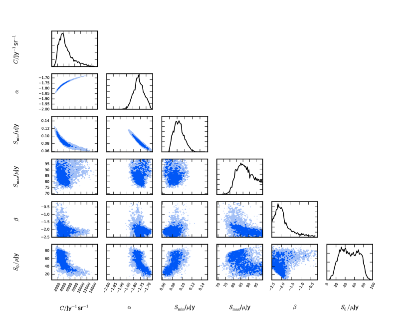
Figure 1: Posterior probability distribution for the (winning) single-break model B fitted to the full SKADS mock catalogue data. The 68 and 95 per cent confidence limits are respectively indicated by the dark and light shaded regions.

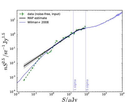
Figure 2: Source counts reconstructed from the SKADS mock catalogue. The underlying, noise-free realisation of the counts for the 1-deg² catalogue is indicated by the green dashed line. The real, noisy catalogue data are shown as a black dashed line. The black line and grey shaded region show the maximum a posteriori (MAP) and 68-per-cent confidence region of the distributions of models reconstructed from every sample from the posterior in Figure 1. The vertical blue lines are at 1$\sigma$ and 5$\sigma$.

To place further constraints on the depth the algorithm can reach, we fixed the position of the faintest break in model C and investigated the effects on the reconstructed counts. Figure 3 shows what happens as the break is positioned at 10, 5, 1 and 0.5 $\mu$Jy. The reconstruction is accurate until it breaks down at $\approx$0.5–1$\mu$Jy, in the sense that the uncertainties suddenly inflate when the enforced break position is decreased to that flux. Note that this is consistent with our assertion above that uncertainties from different bins affect each other, because when the break position is clamped at a very low flux the uncertainties for the lowest flux bins reflect the fact that the counts in this noise-dominated region are independent of the brighter flux bins.

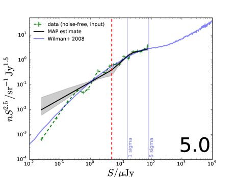
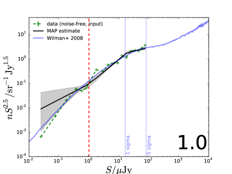
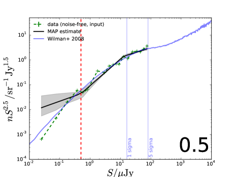
Figure 3: For the SKADS catalogue data, source-count reconstruction for model C as a function of the flux (indicated by the vertical red dashed line) at which the lowest break is fixed: (a) 10, (b) 5, (c) 1 and (d) 0.5 $\mu$Jy. The underlying, noise-free realisation of the counts for the 1-deg² catalogue is indicated by the green dashed line. The real, noisy catalogue data are shown as a black dashed line. The black line and grey shaded region show the maximum a posteriori (MAP) and 68-per-cent confidence region of the distributions of models reconstructed from every sample from the posterior. The vertical blue lines are at 1$\sigma$ and 5$\sigma$.

3.1 Effects of clustering and confusion

Next, in order to account for the effects of clustering and confusion, we injected all the noise-free SKADS sources into a map of noise, synthesized beam, size and pixel size equal to those of the VLA map of section 4.2. Having injected all the noise-free SKADS sources into the map, flux extraction proceeds as in section 4.3, for catalogue positions corresponding to those of injected sources.

For this experiment, we fitted model C (with two breaks) to the binned extracted fluxes. We used model C here because we wanted to allow sufficient freedom in the possibly now-different reconstruction and it was only marginally disfavoured over model B. We carried out the fit with the minimum source flux injected into the map set to be 0.01, 0.1, 0.5 and 1 $\mu$Jy. Figure 4 shows the reconstructions for these different scenarios. With all sources $>$10 nJy injected into the map, the counts are biased high, showing that, if the SKADS simulations portrayed reality, confusion would cause the algorithm to break down when applied to these VLA data even at the 5-$\sigma$ flux limit. Confusion is still an issue (top right in Figure 4) for $S>0.1\mu$Jy, causing the counts to be artificially boosted, but drops away once all sources $<0.5\mu$Jy have been excised from the map (bottom left). This is consistent with the level at which confusion noise is expected in the VLA data (see section 4.2).

While potentially disconcerting, this exercise is useful in understanding the limitations of our modelling scheme. If SKADS is a true representation of the 1.4-GHz sky, our source counts would be biased. If confusion were an issue, efficient deblending algorithms have been proposed (e.g. Kurczynski and Gawiser 2010; Safarzadeh et al. 2015) to mitigate the effects of source blending. We note that this effect may lead to problems for any planned relatively-low-resolution surveys from SKA pathfinders. We return to the effects of confusion in section 5.3.

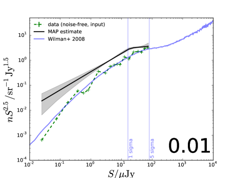
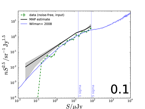
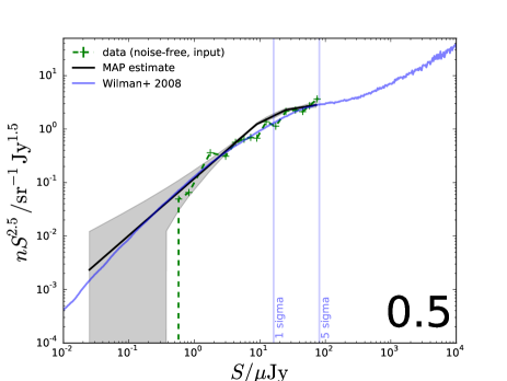
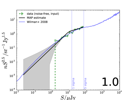
Figure 4: Source-count reconstruction for model C as a function of the minimum flux injected into the map: (a) 0.01, (b) 0.1, (c) 0.5 and (d) 1 $\mu$Jy. The underlying, noise-free realisation of the counts for the 1-deg² catalogue is indicated by the green dashed line. The real, noisy catalogue data are shown as a black dashed line. The black line and grey shaded region show the maximum a posteriori (MAP) and 68-per-cent confidence interval of the distributions of models reconstructed from every sample from the posterior. The vertical blue lines are at 1$\sigma$ and 5$\sigma$.

4 Data

4.1 Infrared and Optical Data

The VIDEO survey (Jarvis et al., 2013), aimed at understanding galaxy formation, evolution and clusters, is ongoing. The data presented here cover $\approx$ 1 square degree and are in $Z,Y,J,H,$ and $K_{\mathrm{s}}\,$bands. The project makes use of Canada–France–Hawaii Telescope Legacy Survey optical data (CFHTLS–D1; Ilbert et al. 2006) in the $u^{*},g^{\prime},r^{\prime},i^{\prime},$ and $z^{\prime}$ bands.

The data selection is similar to that employed by Zwart et al. (2014a). In order to select galaxies solely by stellar mass (see Zwart et al. 2014a and discussion therein), we considered just those with $K_{\mathrm{s}}\,<23.5$, i.e. the 90-per-cent completeness limit for VIDEO’s formal 5-$\sigma$ limit $K_{\mathrm{s}}\,=23.8$ (see Jarvis et al. 2013). We further excised any objects contaminated by detector ghosting halos, as well as any objects that SExtractor deemed to be crowded, blended, saturated, truncated or otherwise corrupted. 71,418 objects remained after this data selection, covering an area of 0.97 sq. deg.

4.2 Radio Data

Radio observations (Bondi et al., 2003) of the VIDEO field cover a 1-square-degree field centred on J 2^h 26^m 00^s  $-$4$\degr$ 30$\arcmin$ 00$\arcsec$ (the XMM–LSS field). The data comprise a 1.4-GHz Very Large Array (VLA, B-array) 9-point mosaic. For any radio mosaicking strategy, the primary beam unavoidably imposes a variation in the map noise (see e.g. AMI Consortium et al. 2011a); for these data this variation is about 20 per cent around $17.5\,\mu$Jy. The clean restoring beam is 6 ″ full width at half maximum and the map contains 2048 $\times$ 2048 1.5-arcsec pixels. In Zwart et al. (2014a) we estimated the expected confusion noise for these 6-arcsec-beam data to be $\sigma^{*}=0.8\,\mu$Jy beam^-1 in the Condon et al. (2012) definition, i.e. about $\sigma_{n}/20$ in our notation.

4.3 Flux extraction

It was pointed out by Stil et al. (2014) that a Nyquist-sampled synthesized beam could be insufficient for a stacking analysis if the positional uncertainty exceeds the width of a pixel. In the present case, the two options were to (i) employ aperture photometry or (ii) resample the map to a finer grid. Since our near-infra-red field is relatively crowded, the first would prove difficult without some deblending scheme (e.g. Kurczynski and Gawiser 2010; Safarzadeh et al. 2015). Hence we selected the second method, upsampling the VLA map by a factor of 8 using interpolation. The scheme was tested on simulations and on the detected sources (i.e. those above $5\sigma$) and the bias in flux density was able to be reduced to $\lesssim 1$ per cent.

A histogram of the extracted fluxes (up to 500 $\mu$Jy) is shown in Figure 5. Although gaussian on the negative side (implying domination by thermal noise), there is a long positive tail caused by discrete radio sources; the tail contains the information that we will exploit to measure the source-count distribution for these sources.

Figure 5: Histogram of the fluxes extracted from the VLA map at the positions of the VIDEO sources. Overlaid with a red dashed curve is a gaussian of width equal to the modal survey noise of 16.2 $\mu$Jy. The vertical blue lines indicate the 1- and 5-$\sigma$ thresholds.

5 Results

With the algorithm and its implementation fully tested and proven, we set about extracting binned source counts at the positions of the VIDEO-detected $K_{\mathrm{s}}\,$-selected sources as described in section 4.3. We used 41 bins in the range $-108<S/\mu$Jy $<85$, with tighter binning near zero to reflect the increased numbers of sources in that flux region.

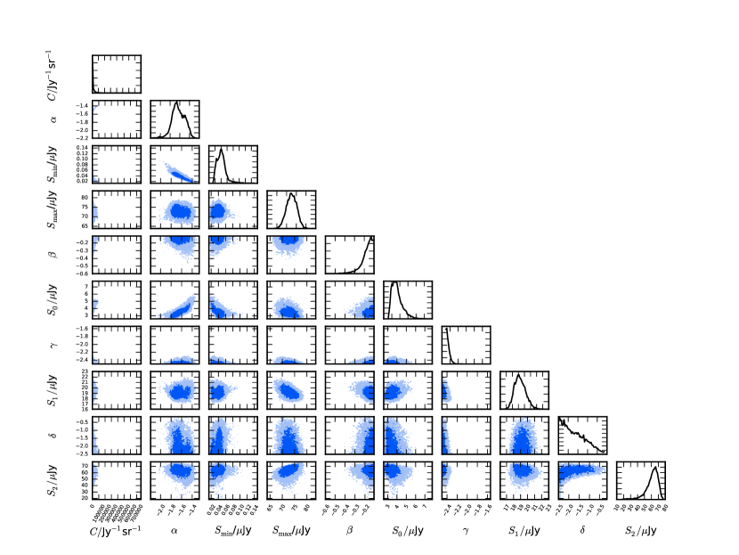
Figure 7: Posterior probability distribution for the three-break model D fitted to the VIDEO data. The dark and light shaded regions indicate the 68 and 95 per cent confidence limits.

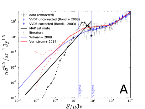
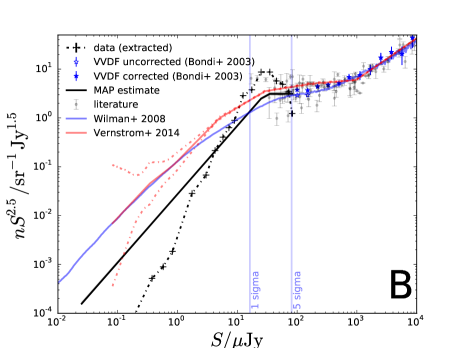
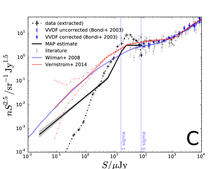
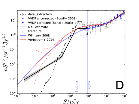
Figure 8: Reconstructions for all galaxies in the VIDEO sample. The model fitted is indicated bottom right. The underlying full SKADS (Wilman et al., 2008) counts are shown in blue, and the only other counts at these depths (Vernstrom et al., 2014) are marked in red, with the 68 per cent confidence interval in dashed red. The filled and empty blue stars respectively represent the Bondi et al. (2003) corrected and uncorrected counts for the VLA $>5\sigma$ sources. Literature values are taken from the review by de Zotti et al. (2010). The real, noisy data are shown as a black dashed line. The black line and grey shaded region show the maximum a posteriori (MAP) and 68-per-cent confidence interval of the distributions of models reconstructed from every sample from the posterior. The vertical blue lines are at 1$\sigma$ and 5$\sigma$.

The relative log_e-evidences (for fixed $\sigma_{n}$) are given in Table 3. The preferred model, i.e. the one with the highest evidence, is model D. The posterior probability distribution for that model is given in Figure 7. Figure 8 shows the reconstructions for the four models. A single power law (model A) has a slope that is consistent with that from Wilman et al. (2008) and Vernstrom et al. (2014), but the amplitude is relatively low and the fit at the bright end is poor. The evidence anyway strongly rejected this model. When a break is added (model B), the fit at the bright end becomes consistent with the $>5\sigma$ counts from Bondi et al. (2003).

The model C and D reconstructions are very similar, and our conclusions remain the same even though D is formally preferred. Taking model C (with two breaks), then, the counts remain flat to just below 20$\mu$Jy ($\simeq 1\sigma$), before falling steeply. After the second break, at around 3$\mu$Jy, the counts become shallower and do not become consistent with those from Wilman et al. (2008) and Vernstrom et al. (2014) again until $<0.5\mu$Jy.

5.1 Sensitivity to thermal-noise contribution

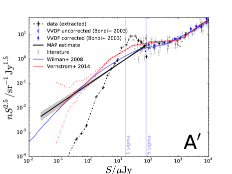
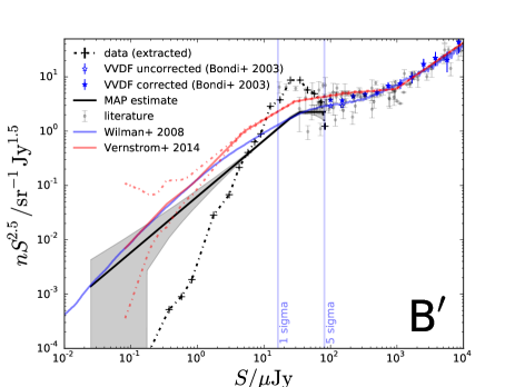
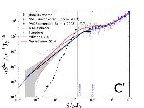
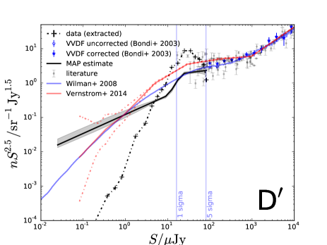
Figure 9: Reconstructions for all galaxies in the VIDEO sample. The model fitted is indicated bottom right, the preferred one being model B′. The underlying full SKADS (Wilman et al., 2008) counts are shown in blue, and the only other counts at these depths (Vernstrom et al., 2014) are marked in red, with the 68 per cent confidence interval in dashed red. The filled and empty blue stars respectively represent the Bondi et al. (2003) corrected and uncorrected counts for the VLA $>5\sigma$ sources. Literature values are taken from the review by de Zotti et al. (2010). The real, noisy data are shown as a black dashed line. The black line and grey shaded region show the maximum a posteriori (MAP) and 68-per-cent confidence interval of the distributions of models reconstructed from every sample from the posterior. The vertical blue lines are at 1$\sigma$ and 5$\sigma$.

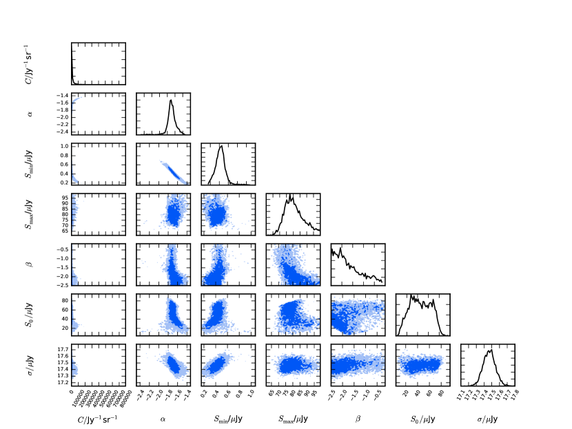
Figure 10: Posterior probability distribution for the preferred three-break model B′ fitted to the VIDEO data. 68 and 95 per cent confidence limits are shown as dark and light blue shaded regions respectively.

As a final check, we repeated the same fitting procedure, but allowing for an extra degree of freedom in that $\sigma_{n}$ was now allowed to vary uniformly in the range $0.5$–$2.0\times\sigma_{\mathrm{survey,modal}}$. This was because there was a hint (see for example Figure 5) that the assumed map noise was an underestimate. Table 4 shows the model-selection results. Immediately one sees that the relative evidences are overwhelmingly higher for this family of models when compared to the fixed-noise set. Model B′ is now the preferred model, though only marginally compared to A′, C′ and D′, but it is nonetheless model B′ that we formally adopt. Figure 9 gives the corresponding reconstructions and Figure 10 is the posterior distribution for model B′. The intermediate break in the counts now disappears, indicating that the earlier models had probably been compensating for an incorrect noise figure, the model now being summarizable as flat to $\approx 40\mu$Jy, then falling with a slope of $-$1.7 below that flux. The map noise estimated via the new route is $17.5\pm 0.08\mu$Jy rather than the modal value of 16.2$\mu$Jy assumed earlier.

5.2 Interpretation

Heywood et al. (2013) showed that the scatter in the counts at 100$\mu$Jy could be attributed to sample variance, but this becomes less true at fainter fluxes as the raw numbers of sources increase, so that it is unclear that this could scatter our counts. Assuming, then, no contribution from sample variance, we might interpret the very slight deficit of radio emission in that region to indicate that some small fraction of the Vernstrom et al. (2014) radio sources are beyond the faintness limit of the VIDEO data. Note that the difference in the counts cannot be due to confusion, since we found earlier that confusion tended to bias the counts upwards. We see also that our inferred source counts are not consistent with those derived from the ARCADE2 data (Seiffert et al. 2011 and Fixsen et al. 2011), which afforded integral constraints on the 3–90-GHz temperature contribution of a putative population of non-Galactic discrete radio sources below some limiting flux, constraining the differential counts to be $\propto S^{-2.6}$, i.e. very flat in the Euclidean normalization. Our results thus give further weight to the argument of Vernstrom et al. (2014) (see their Figure 18) that the ARCADE2 ‘excess’ cannot be accounted for by a population of faint discrete sources.

5.3 Could there be a confusing background?

As a final test, we undertook map extractions at 72,000 random positions for both the SKADS simulations and the VIDEO-VLA data. This should give an indication of the confusion ‘background’ away from the stacked positions. No $>5\sigma$ sources were injected into the SKADS map. In the case of the VIDEO data, we masked out the known (i.e. $>5\sigma$) sources from the Bondi et al. (2003) catalogue using circular apertures of radius $5\times$ the full width at half maximum of the synthesized beam, random pixels being drawn without replacement from the remaining area (subsequently corrected for).

The reconstructions for the preferred models (from a choice of A, B, C and D for SKADS, and from all eight models for VIDEO) fitted to the resulting flux histograms are shown in Figure 2. The comparison is revealing. For the SKADS extraction, the inferred counts are flat in euclidean space, with a very slight ramp at the bright end, with small uncertainties caused by a high signal-to-noise measurement of the average background flux. The VIDEO counts have a ramp at 1–5$\sigma$ due to confusion from unmasked sources in that regime (consider, for example, flux boosting due to an unmasked 4.5$\sigma$ source). However, the overall amplitude is considerably suppressed relative to the signal from the true positions (note the logarithmic scale), even including the ramp. Moreover, the amplitude is suppressed by a factor of $\approx$20 compared to the SKADS prediction. We conclude that our results are not contaminated by confusion at any notable level.

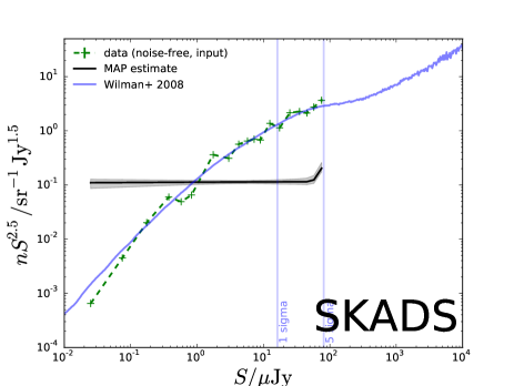
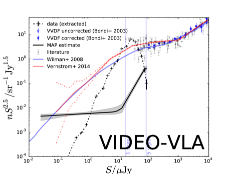
Figure 6: Source-count reconstructions for the preferred models for SKADS (left, model B) and VIDEO (right, model D′) when 72,000 random map positions are used for the stacking. The underlying, noise-free realisation of the counts for the 1-deg² catalogue is indicated by the green dashed line. The real, noisy catalogue data are shown as a black dashed line. The black line and grey shaded region show the maximum a posteriori (MAP) and 68-per-cent confidence interval of the distributions of models reconstructed from every sample from the posterior. The vertical blue lines are at 1$\sigma$ and 5$\sigma$. The underlying full SKADS (Wilman et al., 2008) counts are shown in blue, and the only other counts at these depths (Vernstrom et al., 2014) are marked in red, with the 68 per cent confidence interval in dashed red. The filled and empty blue stars respectively represent the Bondi et al. (2003) corrected and uncorrected counts for the VLA $>5\sigma$ sources. Literature values are taken from the review by de Zotti et al. (2010).

Table 3: Evidences $\Delta\mathcal{Z}$ for models A–D applied to the VIDEO data, relative to model A. It appears that the preferred model at this stage is D, but see Table 4.

Model	$\Delta\log_{\mathrm{e}}\mathcal{Z}$	Odds ratio $\mathcal{Z}/\mathcal{Z}_{A}$
A	0.0	1
B	7.44$\pm$0.22	$10^{3.2}$:1
C	21.24$\pm$0.24	$10^{9.2}$:1
D	27.65$\mathbf{\pm}$0.24	$10^{12.0}$:1

Table 4: Evidences $\Delta\mathcal{Z}$ for models A′–D′ applied to the VIDEO data, relative to model A. The preferred model is now (just) B′.

Model	$\Delta\log_{\mathrm{e}}\mathcal{Z}$	Odds ratio $\mathcal{Z}/\mathcal{Z}_{A}$
A	0.0	1
A′	152.51$\pm$0.21	$10^{66.23}$:1
B′	152.86$\mathbf{\pm}$0.21	$10^{66.39}$:1
C′	152.70$\pm$0.21	$10^{66.32}$:1
D′	152.48$\pm$0.21	$10^{66.22}$:1

5.4 Subdivision by galaxy type

We subdivided the galaxy sample using the criteria of Zwart et al. (2014a), which are based on the best-fitting spectral-energy distribution (to the 10-band photometry), which Zwart et al. argue to be a better discriminator than a colour-colour diagram. The three subsample classifications are (i) ellipticals, (ii) normal (Sbc, Scd, low-mass irregular) galaxies and (iii) starburst galaxies. We fitted models A′–D′ to the three subsamples from this scheme in order to investigate the relative contributions to the source counts of the different populations. The results are summarized in Table 5 and Figure 11. The counts are dominated by the more numerous ‘normal’ galaxies, whose counts also exhibit the (full sample’s) flat behaviour down to $\simeq 20\mu$Jy. The counts of the ellipticals do not flatten at the bright end, but fall at a shallower rate, one that is consistent with the very bright ($>1$ mJy) slope, as expected for such AGN hosts. The starburst counts are not as flat as the overall trend as far as 20$\mu$Jy, but do, like the other subsamples, steepen below that flux. Hence, as expected, the source counts are dominated by normal ‘spiral galaxies’ at these fluxes, with starburst galaxies and AGN making little contribution (our selection excludes QSOs).

Table 5: Summary of analysis for the VIDEO galaxy-type subsamples.

Type	Galaxies	Flux range / $\mu$Jy	Bins	Preferred model
All	71,418	$-$108–85	41	B′
Elliptical	5351	$-$67–85	38	B′
Normal	54,879	$-$108–85	41	C′
Starburst	11,187	$-$69–85	38	B′

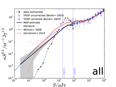
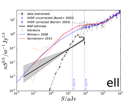
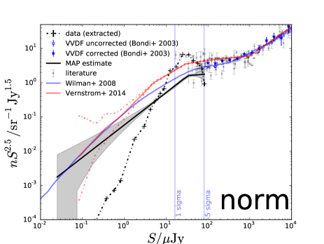
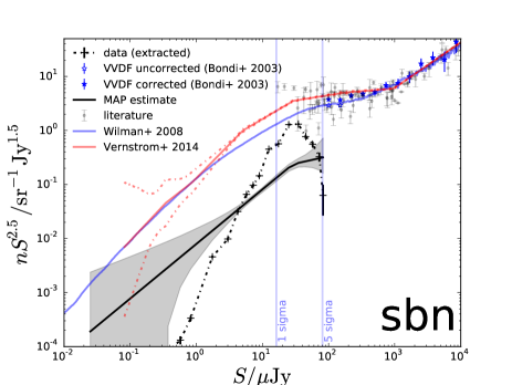
Figure 11: Reconstructions for galaxies in the VIDEO sample, by galaxy subsample (all, elliptical, normal and starburst). The underlying full SKADS (Wilman et al., 2008) counts are shown in blue, and the only other counts at these depths (Vernstrom et al., 2014) are marked in red, with the 68 per cent confidence interval in dashed red. The filled and empty blue stars respectively represent the Bondi et al. (2003) corrected and uncorrected counts for the VLA $>5\sigma$ sources. Literature values are taken from the review by de Zotti et al. (2010). The real, noisy data are shown as a black dashed line. The black line and grey shaded region show the maximum a posteriori (MAP) and 68-per-cent confidence interval of the distributions of models reconstructed from every sample from the posterior. The vertical blue lines are at 1$\sigma$ and 5$\sigma$.

6 Conclusions

1. We have cast ‘sub-threshold stacking’ in a fully bayesian framework for the first time, including the ability to calculate the evidence for the purposes of model selection.

2. As well as the bayesian evidence, our framework reveals the exploration of full posterior probability distributions, showing explicitly any degeneracies and/or correlations. We note that marginalized parameter estimates are incorrect if such degeneracies are present as in these cases.

3. We applied the algorithm to the SKADS simulations. When run on a SKADS catalogue, we were able to reconstruct the counts successfully down to sub-$\mu$Jy levels, i.e. the $5\sigma_{n}/\sqrt{N=375000}$ level. This also holds true when applied to data (below).

4. We used the SKADS catalogue to simulate a VIDEO–VLA-like radio map from which we extracted fluxes at the positions of SKADS sources on which to run the algorithm. We showed that confusion biased the counts high unless we artifically assumed no radio emission below 1 $\mu$Jy. This needs to be accounted for in analysis of data from relatively-low-resolution SKA pathfinders such as ASKAP.

5. We applied the algorithm to VLA data stacked at VIDEO positions. A power-law model (D) with three breaks (the two at 3 $\mu$Jy and 20 $\mu$Jy being the predominant ones) is preferred when the modal map noise of 16.2 $\mu$Jy is assumed.

6. When the map noise is varied as a free parameter, a power-law model (B′) with a single break is overwhelmingly preferred, and we adopt model B′ (over the fixed-noise model D) as our final result. The inferred counts can be summarized as flat to $\approx 40\mu$Jy, then falling with a slope of $-$1.7 below that flux. The map noise estimated via is this route is, rather, $17.5\pm 0.08\mu$Jy.

7. While one would not expect them to match a priori, we interpret the slight deficit of counts below 20 $\mu$Jy relative to the results of Wilman et al. (2008) and Vernstrom et al. (2014) as indicative of a fraction of the radio emission coming from galaxies fainter than the flux limit of the VIDEO catalogue, be they lower-redshift faint galaxies with some ongoing star formation, or higher-redshift moderately bright galaxies. Like those works, our results are not consistent with the ARCADE2 results or indeed those from the work of Owen and Morrison (2008).

8. We have subdivided the VIDEO sample into ellipticals, normal and starburst galaxies, and fitted source count models to the binned flux distributions, finding that the counts are dominated by normal ‘spiral galaxies’ at these fluxes, with little contribution from starburst galaxies or AGN.

9. We note the usefulness and wide applicability of our algorithm, and look forward to its employment in future radio surveys such as those with MeerKAT (Jarvis, 2012), LOFAR (van Haarlem et al., 2013), ASKAP (Norris et al., 2011) and SKA (Norris et al., 2013; Prandoni and Seymour, 2014).

6.1 Future work

The radio luminosity, solely a function of source flux and redshift, can be used to infer star-formation rates, and, using the available stellar-mass estimates, specific star-formation rates (cf. Zwart et al. 2014a). It will be straightforward to extend our algorithm to the derivation of luminosity functions (Malefahlo et al. in prep.), and their evolution with redshift, building on our work and that of Roseboom and Best (2014). It will be interesting to compare estimates for these quantities with those derived from traditional stacking methods. As hinted at earlier, one would like to undertake a joint analysis of the counts of confusing sources below the thermal-noise limit together with those measured in this work, and our framework permits this too. Finally, the algorithm can readily be applied to any survey data map that has an auxiliary catalogue of greater depth and resolution, e.g. VLA-COSMOS, 10C (Whittam et al. in prep.), BLAST or Herschel-ATLAS, though in some low-resolution cases modification may be needed in order to account for a $P(D)$-style confusion contribution (high likelihood of beam occupancy $>$1).

References

- AMI Consortium et al. (2011a) AMI Consortium et al.: 2011a, MNRAS 415, 2699
- AMI Consortium et al. (2011b) AMI Consortium et al.: 2011b, MNRAS 415, 2708
- Becker et al. (1995) Becker, R. H., White, R. L., and Helfand, D. J.: 1995, Astrophys. J. 450, 559
- Bondi et al. (2003) Bondi, M. et al.: 2003, A&A 403, 857
- Bourne et al. (2012) Bourne, N. et al.: 2012, MNRAS 421, 3027
- Bridges et al. (2009) Bridges, M., Feroz, F., Hobson, M. P., and Lasenby, A. N.: 2009, MNRAS 400, 1075
- Buchner et al. (2014) Buchner, J., Georgakakis, A., Nandra, K., Hsu, L., Rangel, C., Brightman, M., Merloni, A., Salvato, M., Donley, J., and Kocevski, D.: 2014, A&A 564, A125
- Condon (1974) Condon, J. J.: 1974, Astrophys. J. 188, 279
- Condon (1992) Condon, J. J.: 1992, ARA&A 30, 575
- Condon et al. (2002) Condon, J. J., Cotton, W. D., and Broderick, J. J.: 2002, A J 124, 675
- Condon et al. (2012) Condon, J. J., Cotton, W. D., Fomalont, E. B., Kellermann, K. I., Miller, N., Perley, R. A., Scott, D., Vernstrom, T., and Wall, J. V.: 2012, Astrophys. J. 758, 23
- de Zotti et al. (2010) de Zotti, G., Massardi, M., Negrello, M., and Wall, J.: 2010, Astronomy & Astrophysics Review 18, 1
- Dunne et al. (2009) Dunne, L., Ivison, R. J., Maddox, S., Cirasuolo, M., Mortier, A. M., Foucaud, S., Ibar, E., Almaini, O., Simpson, C., and McLure, R.: 2009, MNRAS 394, 3
- Feroz et al. (2011) Feroz, F., Balan, S. T., and Hobson, M. P.: 2011, MNRAS 416, L104
- Feroz and Hobson (2008) Feroz, F. and Hobson, M. P.: 2008, MNRAS 384, 449
- Feroz et al. (2009a) Feroz, F., Hobson, M. P., and Bridges, M.: 2009a, MNRAS 398, 1601
- Feroz et al. (2009b) Feroz, F., Hobson, M. P., Zwart, J. T. L., Saunders, R. D. E., and Grainge, K. J. B.: 2009b, MNRAS 398, 2049
- Fixsen et al. (2011) Fixsen, D. J., Kogut, A., Levin, S., Limon, M., Lubin, P., Mirel, P., Seiffert, M., Singal, J., Wollack, E., Villela, T., and Wuensche, C. A.: 2011, Astrophys. J. 734, 5
- Franzen et al. (2014) Franzen, T. M. O., Sadler, E. M., Chhetri, R., Ekers, R. D., Mahony, E. K., Murphy, T., Norris, R. P., Waldram, E. M., and Whittam, I. H.: 2014, MNRAS 439, 1212
- Hales et al. (2014a) Hales, C. A., Norris, R. P., Gaensler, B. M., and Middelberg, E.: 2014a, MNRAS 440, 3113
- Hales et al. (2014b) Hales, C. A., Norris, R. P., Gaensler, B. M., Middelberg, E., Chow, K. E., Hopkins, A. M., Huynh, M. T., Lenc, E., and Mao, M. Y.: 2014b, MNRAS 441, 2555
- Hewish (1961) Hewish, A.: 1961, MNRAS 123, 167
- Heywood et al. (2013) Heywood, I., Jarvis, M. J., and Condon, J. J.: 2013, MNRAS 432, 2625
- Ilbert et al. (2006) Ilbert, O. et al.: 2006, A&A 457, 841
- Jarvis (2012) Jarvis, M. J.: 2012, African Skies 16, 44
- Jarvis et al. (2013) Jarvis, M. J. et al.: 2013, MNRAS 428, 1281
- Karim et al. (2011) Karim, A., Schinnerer, E., Martínez-Sansigre, A., Sargent, M. T., van der Wel, A., Rix, H.-W., Ilbert, O., Smolčić, V., Carilli, C., Pannella, M., Koekemoer, A. M., Bell, E. F., and Salvato, M.: 2011, Astrophys. J. 730, 61
- Komatsu et al. (2011) Komatsu, E. et al.: 2011, ApJ Suppl. 192, 18
- Kurczynski and Gawiser (2010) Kurczynski, P. and Gawiser, E.: 2010, A J 139, 1592
- Lochner et al. (2015) Lochner, M., Natarajan, I., Zwart, J. T. L., Smirnov, O., Bassett, B. A., Oozeer, N., and Kunz, M.: 2015, astro-ph.IM/1501.05304
- MacKay (2003) MacKay, D.: 2003, Information Theory, Inference and Learning Algorithms, Cambridge: CUP
- Mahony et al. (2011) Mahony, E. K., Sadler, E. M., Croom, S. M., Ekers, R. D., Bannister, K. W., Chhetri, R., Hancock, P. J., Johnston, H. M., Massardi, M., and Murphy, T.: 2011, MNRAS 417, 2651
- Marsden et al. (2009) Marsden, G. et al.: 2009, Astrophys. J. 707, 1729
- Massardi et al. (2011) Massardi, M. et al.: 2011, MNRAS 412, 318
- Mitchell-Wynne et al. (2014) Mitchell-Wynne, K., Santos, M. G., Afonso, J., and Jarvis, M. J.: 2014, MNRAS 437, 2270
- Norris et al. (2011) Norris, R. P. et al.: 2011, PASA 28, 215
- Norris et al. (2013) Norris, R. P. et al.: 2013, PASA 30, 20
- Owen and Morrison (2008) Owen, F. N. and Morrison, G. E.: 2008, A J 136, 1889
- Patanchon et al. (2009) Patanchon, G. et al.: 2009, Astrophys. J. 707, 1750
- Prandoni and Seymour (2014) Prandoni, I. and Seymour, N.: 2014, Advancing Astrophysics with the Square Kilometre Array, Chapt. Revealing the Physics and Evolution of Galaxies and Galaxy Clusters with SKA Continuum Surveys, astro-ph.IM/1412.6512, POS
- Roseboom and Best (2014) Roseboom, I. G. and Best, P. N.: 2014, MNRAS 439, 1286
- Safarzadeh et al. (2015) Safarzadeh, M., Ferguson, H. C., Lu, Y., Inami, H., and Somerville, R. S.: 2015, Astrophys. J. 798, 91
- Scheuer (1957) Scheuer, P. A. G.: 1957, in Proceedings of the Cambridge Philisophical Society, pp 764–773
- Scoville et al. (2007) Scoville, N., Aussel, H., Brusa, M., Capak, P., Carollo, C. M., Elvis, M., Giavalisco, M., Guzzo, L., Hasinger, G., Impey, C., Kneib, J.-P., LeFevre, O., Lilly, S. J., Mobasher, B., Renzini, A., Rich, R. M., Sanders, D. B., Schinnerer, E., Schminovich, D., Shopbell, P., Taniguchi, Y., and Tyson, N. D.: 2007, ApJ Suppl. 172, 1
- Seiffert et al. (2011) Seiffert, M., Fixsen, D. J., Kogut, A., Levin, S. M., Limon, M., Lubin, P. M., Mirel, P., Singal, J., Villela, T., Wollack, E., and Wuensche, C. A.: 2011, Astrophys. J. 734, 6
- Seymour et al. (2008) Seymour, N., Dwelly, T., Moss, D., McHardy, I., Zoghbi, A., Rieke, G., Page, M., Hopkins, A., and Loaring, N.: 2008, MNRAS 386, 1695
- Skilling (2004) Skilling, J.: 2004, in R. Fischer, R. Preuss, and U. V. Toussaint (eds.), American Institute of Physics Conference Series, pp 395–405
- Stil et al. (2014) Stil, J. M., Keller, B. W., George, S. J., and Taylor A. R.: 2014, Astrophys. J. 787, 99
- van Haarlem et al. (2013) van Haarlem, M. P. et al.: 2013, A&A 556, A2
- Vernstrom et al. (2014) Vernstrom, T., Scott, D., Wall, J. V., Condon, J. J., Cotton, W. D., Fomalont, E. B., Kellermann, K. I., Miller, N., and Perley, R. A.: 2014, MNRAS 440, 2791
- Whittam et al. (2013) Whittam, I. H., Riley, J. M., Green, D. A., Jarvis, M. J., Prandoni, I., Guglielmino, G., Morganti, R., Röttgering, H. J. A., and Garrett, M. A.: 2013, MNRAS 429, 2080
- Wilman et al. (2008) Wilman, R. J. et al.: 2008, MNRAS 388, 1335
- Wilman et al. (2010) Wilman, R. J., Jarvis, M. J., Mauch, T., Rawlings, S., and Hickey, S.: 2010, astro-ph.CO/1002.1112
- Zwart et al. (2011) Zwart, J. T. L. et al.: 2011, MNRAS 418, 2754
- Zwart et al. (2014a) Zwart, J. T. L., Jarvis, M. J., Deane, R. P., Bonfield, D. G., Knowles, K., Madhanpall, N., Rahmani, H., and Smith, D. J. B.: 2014a, MNRAS 439, 1459
- Zwart et al. (2014b) Zwart, J. T. L., Wall, J., Karim, A., Jackson, C., Norris, R., Condon, J., Afonso, J., Heywood, I., Jarvis, M., Navarrete, F., Prandoni, I., Rigby, E., Rottgering, H., Santos, M., Sargent, M., Seymour, N., Taylor, R., and Vernstrom, T.: 2014b, Advancing Astrophysics with the Square Kilometre Array, Chapt. Astronomy below the Survey Threshold, astro-ph.GA/1412.5743, POS