Pseudospectra of the Schrödinger operator with a discontinuous complex potential

Abstract

We study spectral properties of the Schrödinger operator with an imaginary sign potential on the real line. By constructing the resolvent kernel, we show that the pseudospectra of this operator are highly non-trivial, because of a blow-up of the resolvent at infinity. Furthermore, we derive estimates on the location of eigenvalues of the operator perturbed by complex potentials. The overall analysis demonstrates striking differences with respect to the weak-coupling behaviour of the Laplacian.

• pseudospectra, non-self-adjointness, Schrödinger operators, discontinuous potential, weak coupling, Birman-Schwinger principle

• 34L15, 47A10, 47B44, 81Q12

1 Introduction

Extensive work has been done recently in understanding the spectral properties of non-self-adjoint operators through the concept of pseudospectrum. Referring to by now classical monographs by Trefethen and Embree [33] and Davies [8], we define the pseudospectrum of an operator $T$ in a Hilbert space $\mathcal{H}$ to be the collection of sets

$$\sigma_{\varepsilon}(T):=\sigma(T)\cup\left\{z\in\mathbb{C}:\,\|(T-z)^{-1}\|>\varepsilon^{-1}\right\}\,,$$ (1.1)

parametrised by $\varepsilon>0$, where $\|\cdot\|$ is the operator norm of $\mathcal{H}$. If $T$ is self-adjoint (or more generally normal), then $\sigma_{\varepsilon}(T)$ is just an $\varepsilon$-tubular neighbourhood of the spectrum $\sigma(T)$. Universally, however, the pseudospectrum is a much more reliable spectral description of $T$ than the spectrum itself. For instance, it is the pseudospectrum that measures the instability of the spectrum under small perturbations by virtue of the formula

$$\sigma_{\varepsilon}(T)=\bigcup_{\|U\|\leq 1}\sigma(T+\varepsilon U)\,.$$ (1.2)

Leaving aside a lot of other interesting situations, let us recall the recent results when $T$ is a differential operator. As a starting point we take the harmonic-oscillator Hamiltonian with complex frequency, which is also known as the rotated or Davies’ oscillator (see [8, Sec. 14.5] for a review and references). Although the complexification has a little effect on the spectrum (the eigenvalues are just rotated in the complex plane), a careful spectral analysis reveals drastic changes in basis and other more delicate spectral properties of the operator, in particular, the spectrum is highly unstable against small perturbations, as a consequence of the pseudospectrum containing regions very far from the spectrum. Similar peculiar spectral properties have been established for complex anharmonic oscillators (to the references quoted in [8, Sec. 14.5], we add [15, 24] for the most recent results), quadratic elliptic operators [27, 17, 34], complex cubic oscillators [30, 16, 21, 26], and other models (see the recent survey [21] and references therein).

A distinctive property of the complexified harmonic oscillator is that the associated spectral problem is explicitly solvable in terms of special functions. A powerful tool to study the pseudospectrum in the situations where explicit solutions are not available is provided by microlocal analysis [7, 39, 11]. The weak point of the semiclassical methods is the usual hypothesis that the coefficients of the differential operator are smooth enough (e.g. the potential of the Schrödinger operator must be at least continuous), and it is indeed the case of all the models above. Another common feature of the differential operators whose pseudospectrum has been analysed so far is that their spectrum consists of discrete eigenvalues only.

The objective of the present work is to enter an unexplored area of the pseudospectral world by studying the pseudospectrum of a non-self-adjoint Schrödinger operator whose potential is discontinuous and, at the same time, such that the essential spectrum is not empty. Among various results described below, we prove that the pseudospectrum is non-trivial, despite the boundedness of the potential. Namely, we show that the norm of the resolvent can become arbitrarily large outside a fixed neighbourhood of its spectrum. We hope that our results will stimulate further analysis of non-self-adjoint differential operators with singular coefficients.

2 Main results

In this section we introduce our model and collect the main results of the paper. The rest of the paper is primarily devoted to proofs, but additional results can be found there, too.

2.1 The model

Motivated by the role of step-like potentials as toy models in quantum mechanics, in this paper we consider the Schrödinger operator in $L^{2}(\mathbb{R})$ defined by

$$H:=-\frac{d^{2}}{dx^{2}}+i\,\mathop{\mathrm{sgn}}\nolimits(x)\,,\qquad\mathsf{Dom}(H):=W^{2,2}(\mathbb{R})\,.$$ (2.1)

In fact, $H$ can be considered as an infinite version of the $\mathcal{PT}$-symmetric square well introduced in [37] and further investigated in [38, 29].

Note that $H$ is obtained as a bounded perturbation of the (self-adjoint) Hamiltonian of a free particle in quantum mechanics, which we shall simply denote here by $-\Delta$. Consequently, $H$ is well defined (i.e. closed and densely defined). In fact, $H$ is m-sectorial with the numerical range (defined, as usual, by the set of all complex numbers $(\psi,H\psi)$ such that $\psi\in\mathsf{Dom}(H)$ and $\|\psi\|=1$) coinciding with the closed half-strip

$$\mathsf{Num}(H)=\overline{\mathcal{S}}\,,\qquad\mbox{where}\qquad\mathcal{S}:=[0,+\infty)+i\,(-1,1)\,.$$ (2.2)

The adjoint of $H$, denoted here by $H^{*}$, is simply obtained by changing $+i$ to $-i$ in (2.1). Consequently, $H$ is neither self-adjoint nor normal. However, it is $\mathcal{T}$-self-adjoint (i.e. $H^{*}=\mathcal{T}H\mathcal{T}$), where $\mathcal{T}$ is the antilinear operator of complex conjugation (i.e. $\mathcal{T}\psi:=\overline{\psi}$). At the same time, $H$ is $\mathcal{P}$-self-adjoint, where $\mathcal{P}$ is the parity operator defined by $(\mathcal{P}\psi)(x):=\psi(-x)$. Finally, $H$ is $\mathcal{PT}$-symmetric in the sense of the validity of the commutation relation $[H,\mathcal{PT}]=0$.

Due to the analogy of the time-dependent Schrödinger equation for a quantum particle subject to an external electromagnetic field and the paraxial approximation for a monochromatic light propagation in optical media [23], the dynamics generated by (2.1) can experimentally be realised using optical systems. The physical significance of $\mathcal{PT}$-symmetry is a balance between gain and loss [5].

2.2 The spectrum

As a consequence of (2.2), the spectrum of $H$ is contained in $\overline{\mathcal{S}}$. Moreover, the $\mathcal{PT}$-symmetry implies that the spectrum is symmetric with respect to the real axis. By constructing the resolvent of $H$ and employing suitable singular sequences for $H$, we shall establish the following result.

Proposition 2.1.

We have

$$\sigma(H)=\sigma_{\mathrm{ess}}(H)=[0,+\infty)+i\,\{-1,+1\}\,.$$ (2.3)

The fact that the two rays $[0,+\infty)\pm i$ form the essential spectrum of $H$ is expectable, because they coincide with the spectrum of the shifted Laplacian $-\Delta\pm i$ in $L^{2}(\mathbb{R})$ and the essential spectrum of differential operators is known to depend on the behaviour of their coefficients at infinity only (cf. [12, Sec. X]). The absence of spectrum outside the rays is less obvious.

In fact, the spectrum in (2.3) is purely continuous, i.e. $\sigma(H)=\sigma_{\mathrm{c}}(H)$, for it can be easily checked that no point from the set on the right hand side of (2.3) can be an eigenvalue of $H$ (as well as $H^{*}$). An alternative way how to a priori show the absence of the residual spectrum of $H$, $\sigma_{\mathrm{r}}(H)$, is to employ the $\mathcal{T}$-self-adjointness of $H$ (cf. [20, Sec. 5.2.5.4]).

2.3 The pseudospectrum

Before stating the main results of this paper, let us recall that a closed operator $T$ is said to have trivial pseudospectra if, for some positive constant $\kappa$, we have

$$\forall\varepsilon>0\,,\qquad\sigma_{\varepsilon}(T)\subset\left\{z:\,\mathop{\mathrm{dist}}\nolimits\big{(}z,\sigma(T)\big{)}\leq\kappa\,\varepsilon\right\}\,,$$

or equivalently,

$$\forall z\in\mathbb{C}\setminus\sigma(T)\,,\qquad\|(T-z)^{-1}\|\leq\frac{\kappa}{\mathop{\mathrm{dist}}\nolimits\big{(}z,\sigma(T)\big{)}}\,.$$ (2.4)

Normal operators have trivial pseudospectra, because for them the equality holds in (2.4) with $\kappa=1$.

In view of (2.2), in our case (2.4) holds with $\kappa=1$ if the resolvent set is replaced by $\mathbb{C}\setminus\overline{\mathcal{S}}$. However, the following statement implies that (2.4) cannot hold inside the half-strip $\mathcal{S}$.

Theorem 2.2.

For all $\varepsilon>0$, there exists a positive constant $r_{0}$ such that, for all $z\in\mathcal{S}$ with ${\rm Re\,}z\geq r_{0}$,

$$(1-\varepsilon)\,\frac{{\rm Re\,}z}{\sqrt{1-({\rm Im\,}z)^{2}}}\leq\|(H-z)^{-1}\|\leq 4\,(1+\varepsilon)\,\frac{{\rm Re\,}z}{1-|{\rm Im\,}z|}\,.$$ (2.5)

Although the estimates give a rather good description of the qualitative shape of the pseudospectra, the constants and dependence on $\mathop{\mathrm{dist}}\nolimits(z,\sigma(H))=1-|{\rm Im\,}z|$ for $z\in\mathcal{S}$ are presumably not sharp.

In view of Theorem 2.2, $H$ represents another example of a $\mathcal{PT}$-symmetric operator with non-trivial pseudospectra. The present study can be thus considered as a natural continuation of the recent works [30, 16, 21]. However, let us stress that the complex perturbation in the present model is bounded. Moreover, comparing the present setting with the situation when (2.1) is subject to an extra Dirichlet condition at zero (cf. Section 7.3), the difference between these two realisations is indeed seen on the pseudospectral level only.

Even though the step-like shape of the potential in (2.1) is a feature of the present study, we stress that the discontinuity by itself is not the source of the non-trivial pseudospectra, see Remark 4.1 below.

The pseudospectrum of $H$ computed numerically using Eigtool [36] by Mark Embree is presented in Figure 1.

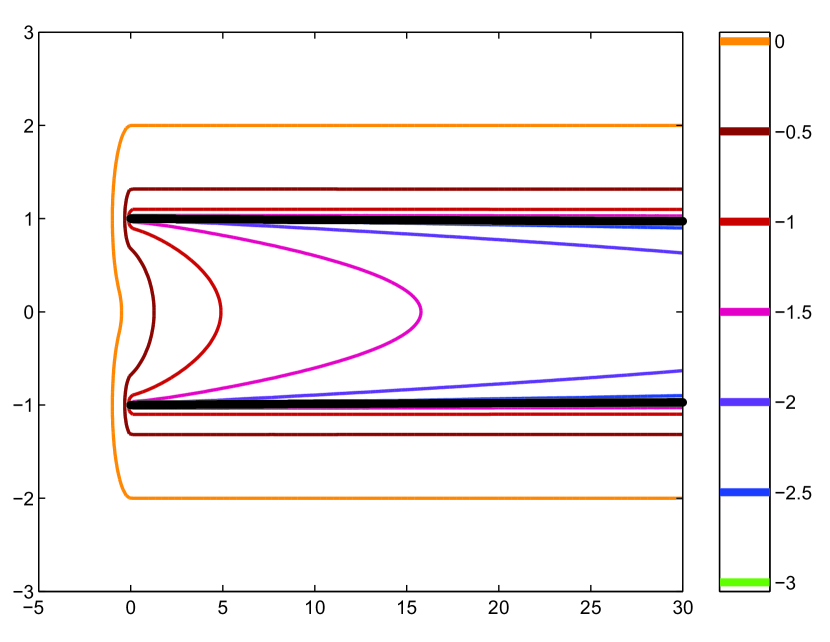
Figure 1: The curves $\|(H-z)^{-1}\|=\varepsilon^{-1}$ in the complex $z$-plane computed for several values of $\varepsilon$; the different colours correspond to $\log_{10}\varepsilon$, while the thick black lines are the essential spectrum of $H$. (Courtesy of Mark Embree.)

2.4 Weak coupling

Inspired by (1.2), we eventually consider the perturbed operator

$$H_{\varepsilon}:=H\,\dot{+}\,\varepsilon V$$ (2.6)

in the limit as $\varepsilon\to 0$. Here $V$ is the operator of multiplication by a function $V\in L^{1}(\mathbb{R})$ that we denote by the same letter. Since $V$ is not necessarily relatively bounded with respect to $H$, the dotted sum in (2.6) is understood in the sense of forms. We remark that the perturbation does not change the essential spectrum, i.e., $\sigma_{\mathrm{ess}}(H_{\varepsilon})=\sigma_{\mathrm{ess}}(H)$, and recall Proposition 2.1.

If $H$ were the free Hamiltonian $-\Delta$ and $V$ were real-valued, the problem (2.6) with $\varepsilon\to 0$ is known as the regime of weak coupling in quantum mechanics. In that case, it is well known that (under some extra assumptions on $V$) the perturbed operator $-\Delta\,\dot{+}\,\varepsilon V$ possesses a unique discrete eigenvalue for all small positive $\varepsilon$ if, and only if, the integral of $V$ is non-positive (see [32] for the original work). This robust existence of “weakly coupled bound states” is of course related to the singularity of the resolvent kernel of the free Hamiltonian at the bottom of the essential spectrum. Indeed, these bound states do not exist in three and higher dimensions, which is in turn related to the validity of the Hardy inequality for the free Hamiltonian (see, e.g., [35]).

Complex-valued perturbations of the free Hamiltonian have been intensively studied in recent years [1, 14, 6, 22, 9, 13, 10]. In [4, 25] the authors consider perturbations of an operator which is by itself non-self-adjoint. In all of these papers, however, the results are inherited from properties of the resolvent of the free Hamiltonian.

In the present setting, the unperturbed operator $H$ is non-self-adjoint. Moreover, its resolvent kernel has no local singularity, but it blows up as $|z|\rightarrow+\infty$ when $|{\rm Im\,}z|<1$, see Section 3. Consequently, discrete eigenvalues of $H_{\varepsilon}$ can only “emerge from the infinity”, but not from any finite point of (2.3). The statement is made precise by virtue of the following result.

Theorem 2.3.

Let $V\in L^{1}\big{(}\mathbb{R},(1+x^{2})\,dx\big{)}$. There exists a positive constant $C$ (independent of $V$ and $\varepsilon$) such that, whenever

$$\varepsilon\,\big{\|}(1+|\cdot|^{2})V\|_{L^{1}(\mathbb{R})}\leq\frac{1}{C}\,,$$

we have

$$\sigma_{\mathrm{p}}(H_{\varepsilon})\subset\overline{\mathcal{S}}\cap\left\{{\rm Re\,}z\geq\frac{C}{\,\varepsilon^{2}\,\|V\|_{L^{1}(\mathbb{R})}^{2}}\right\}\,.$$ (2.7)

It is interesting to compare this estimate on the location of possible eigenvalues of $H_{\varepsilon}$ with the celebrated result of [1]

$$\sigma_{\mathrm{p}}(-\Delta\,\dot{+}\,\varepsilon V)\subset\left\{|z|\leq\frac{\,\varepsilon^{2}\,\|V\|_{L^{1}(\mathbb{R})}^{2}}{4}\right\}\,.$$ (2.8)

Our bound (2.7) can be indeed read as an inverse of (2.8). It demonstrates how much the present situation differs from the study of weakly coupled eigenvalues of the free Hamiltonian.

Under some additional assumptions on $V$, the claim of Theorem 2.3 can be improved in the following way.

Theorem 2.4.

Let $n\geq 2$ and $V\in L^{1}\big{(}\mathbb{R},(1+x^{2n})\,dx\big{)}\cap W^{1,1}(\mathbb{R})$. There exist positive constants $\varepsilon_{0}$ and $C$ such that, for all $\varepsilon\in(0,\varepsilon_{0})$, we have

$$\sigma_{\mathrm{p}}(H_{\varepsilon})\subset\overline{\mathcal{S}}\cap\left\{{\rm Re\,}z\geq\frac{C}{\,\varepsilon^{2n}\,}\right\}\,.$$ (2.9)

In particular, if for instance $V$ belongs to the Schwartz space $\mathscr{S}(\mathbb{R})$, then every eigenvalue $\lambda(\varepsilon)$ of $H_{\varepsilon}$ must “escape to infinity” faster than any power of $\varepsilon^{-1}$ as $\varepsilon\to 0$, namely $|\lambda(\varepsilon)|^{-1}=\mathcal{O}(\varepsilon^{\infty})$.

Remark 2.5.

The reader will notice that statement (2.7) differs from (2.9) in that the latter does not highlight the dependence of the right hand side on the potential $V$ but only on its amplitude $\varepsilon$. The reason is that it is the behaviour of $H_{\varepsilon}$ on diminishing $\varepsilon$ that primarily interests us. Moreover, the proofs of the theorems are different and it would be cumbersome (but doable in principle) to gather the dependence of the right hand side in (2.9) on (different) norms of $V$.

2.5 The content of the paper

The organisation of this paper is as follows.

In Section 3, we find the integral kernel of the resolvent $(H-z)^{-1}$, cf. Proposition 3.1, and use it to prove Proposition 2.1.

In Section 4, the explicit formula of the resolvent kernel is further exploited in order to prove Theorem 2.2.

The definition of the perturbed operator (2.6) and its general properties are established in Section 5. In particular, we locate its essential spectrum (Proposition 5.5) and prove the Birman-Schwinger principle (Theorem 5.3).

Section 6 is divided into two respective subsections, in which we prove Theorems 2.3 and 2.4 with help of the Birman-Schwinger principle and, again, using the explicit formula of the resolvent kernel.

Finally, in Section 7, we present two concrete examples of the perturbed operator (2.6). Moreover, we make a comparison of the present study with a decoupled model due to an extra Dirichlet condition.

3 The resolvent and spectrum

Our goal in this section is to obtain an integral representation of the resolvent of $H$. Using that result, we give a proof of Proposition 2.1.

In the following, we set

$$k_{+}(z):=\sqrt{i-z}\qquad\mbox{and}\qquad k_{-}(z):=\sqrt{-i-z}\,,$$

where we choose the principal value of the square root, i.e., $z\mapsto\sqrt{z}$ is holomorphic on $\mathbb{C}\setminus(-\infty,0]$ and positive on $(0,+\infty)$.

Proposition 3.1.

For all $z\notin\mathbb{R}_{+}+i\,\{-1,1\}\,$, $H-z$ is invertible and, for every $f\in L^{2}(\mathbb{R})\,$,

$$[(H-z)^{-1}f](x)=\int_{\mathbb{R}}\mathcal{R}_{z}(x,y)\,f(y)\,dy\,,$$ (3.1)

where

$$\mathcal{R}_{z}(x,y):=\left\{\begin{aligned} &\frac{1}{k_{+}(z)+k_{-}(z)}\,e^{-k_{\pm}(z)|x|-k_{\mp}(z)|y|}\,,&\pm x\geq 0\,,\,\pm y\leq 0\,,\\ &\frac{1}{2k_{\pm}(z)}\,e^{-k_{\pm}(z)|x-y|}&\\ &\quad\pm\frac{k_{+}(z)-k_{-}(z)}{2k_{\pm}(z)\big{(}k_{+}(z)+k_{-}(z)\big{)}}\,e^{-k_{\pm}(z)|x+y|}\,,&\pm x\geq 0\,,\,\pm y\geq 0\,.\end{aligned}\right.$$ (3.2)

Remark 3.2.

The kernel $\mathcal{R}_{z}(x,y)$ is clearly bounded for every $(x,y)\in\mathbb{R}^{2}$ and fixed $z\not=\pm i$. Moreover, using (4.1) below, it can be shown that it remains bounded for $z=\pm i$ as well. Hence, contrary to the case of the resolvent kernel of the free Hamiltonian $-\Delta$ in one or two dimensions, the resolvent kernel of $H$ has no local singularity. On the other hand, and again contrary to the case of the Laplacian, for all fixed $(x,y)\in\mathbb{R}^{2}$, $|\mathcal{R}_{z}(x,y)|\longrightarrow+\infty$ as ${\rm Re\,}z\rightarrow+\infty$, $z\in\mathcal{S}$. Hence, the kernel exhibits a blow-up at infinity. The absence of singularity will play a fundamental role in the analysis of weakly coupled eigenvalues in Section 6. Moreover, we shall see in Section 4 that the singular behaviour at infinity is responsible for the spectral instability of $H$.

Proof of Proposition 3.1.

Let $z\notin[0,\infty)+i\{-1,1\}$ and $f\in L^{2}(\mathbb{R})$. We look for the solution of the resolvent equation $(H-z)u=f$.

The general solutions $u_{\pm}$ of the individual equations

$$-u^{\prime\prime}+(\pm i-z)u-f=0\qquad\mbox{in}\qquad\mathbb{R}_{\pm}\,,$$ (3.3)

where $\mathbb{R}_{+}:=[0,+\infty)$ and $\mathbb{R}_{-}:=(-\infty,0]$, are given by

$$u_{\pm}(x)=\alpha_{\pm}(x)\,e^{k_{\pm}(z)x}+\beta_{\pm}(x)\,e^{-k_{\pm}(z)x}\,,$$

where $\alpha_{\pm}$, $\beta_{\pm}$ are functions to be yet determined. Variation of parameters leads to the following system:

$$\left\{\begin{array}[]{lll}\alpha_{\pm}^{\prime}(x)e^{k_{\pm}(z)x}+\beta_{\pm}^{\prime}(x)e^{-k_{\pm}(z)x}&=&0\,,\\ k_{\pm}(z)\alpha_{\pm}^{\prime}(x)e^{k_{\pm}(z)x}-k_{\pm}(z)\beta_{\pm}^{\prime}(x)e^{-k_{\pm}(z)x}&=&-f\,.\end{array}\right.$$

Hence, we can choose

$$\alpha_{\pm}(x) =-\frac{1}{2k_{\pm}(z)}\int_{0}^{x}f(y)\,e^{-k_{\pm}(z)y}dy+A_{\pm}\,, \pm x>0\,,$$

$$\beta_{\pm}(x) =\frac{1}{2k_{\pm}(z)}\int_{0}^{x}f(y)\,e^{k_{\pm}(z)y}dy+B_{\pm}\,, \pm x>0\,,$$

where $A_{\pm},B_{\pm}$ are arbitray complex constants. The desired general solutions of (3.3) are then given by

$$u_{\pm}(x)=\frac{-1}{k_{\pm}(z)}\int_{0}^{x}f(y)\,\sinh\big{(}k_{\pm}(z)(x-y)\big{)}\,dy+A_{\pm}e^{k_{\pm}(z)x}+B_{\pm}e^{-k_{\pm}(z)x}\,,$$ (3.4)

with $(A_{+},A_{-},B_{+},B_{-})\in\mathbb{C}^{4}\,$.

Among these solutions, we are interested in those which satisfy the regularity conditions

$$u_{+}(0)=u_{-}(0)\,,\qquad u_{+}^{\prime}(0)=u_{-}^{\prime}(0)\,.$$ (3.5)

These conditions are equivalent to the system

$$\left\{\begin{array}[]{ccc}A_{+}+B_{+}&=&A_{-}+B_{-}\,,\\ k_{+}(z)A_{+}-k_{+}(z)B_{+}&=&k_{-}(z)A_{-}-k_{-}(z)B_{-}\,,\end{array}\right.$$

whence we obtain the following relations:

$$\left\{\begin{array}[]{ccc}2A_{+}&=&\big{(}k_{+}(z)+k_{-}(z)\big{)}A_{-}+\big{(}k_{+}(z)-k_{-}(z)\big{)}B_{-}\,,\\ 2B_{+}&=&\big{(}k_{+}(z)-k_{-}(z)\big{)}A_{-}+\big{(}k_{+}(z)+k_{-}(z)\big{)}B_{-}\,.\end{array}\right.$$ (3.6)

Summing up, assuming (3.6), the function

$$u(x):=\begin{cases}u_{+}(x)&\mbox{if}\quad x\geq 0\,,\\ u_{-}(x)&\mbox{if}\quad x\leq 0\,,\end{cases}$$ (3.7)

belongs to $W_{\mathrm{loc}}^{2,2}(\mathbb{R})$ and solves the differential equation (3.3) in the whole $\mathbb{R}$. It remains to check some decay conditions as $x\rightarrow\pm\infty$ in addition to (3.6). This can be done by setting

$$A_{+} :=\frac{1}{2k_{+}(z)}\int_{0}^{+\infty}f(y)\,e^{-k_{+}(z)y}dy\,,$$ (3.8)

$$B_{-} :=\frac{1}{2k_{-}(z)}\int_{-\infty}^{0}f(y)\,e^{k_{-}(z)y}dy\,.$$ (3.9)

Indeed, then

$$u_{+}(x) = -\frac{1}{2k_{+}(z)}\,e^{k_{+}(z)x}\int_{x}^{+\infty}f(y)\,e^{-k_{+}(z)y}dy$$

$$+e^{-k_{+}(z)x}\left(\frac{1}{2k_{+}(z)}\int_{0}^{x}f(y)\,e^{k_{+}(z)y}dy+B_{+}\right)$$

goes to $0$ as $x\rightarrow+\infty$, and similarly for $u_{-}$.

By gathering relations (3.6), (3.8) and (3.9), we obtain the following values for $A_{-}$ and $B_{+}$:

$$A_{-}=\ \frac{1}{k_{+}(z)+k_{-}(z)}\int_{0}^{+\infty}f(y)\,e^{-k_{+}(z)y}dy$$

$$-\frac{k_{+}(z)-k_{-}(z)}{2k_{-}(z)\big{(}k_{+}(z)+k_{-}(z)\big{)}}\int_{-\infty}^{0}f(y)\,e^{k_{-}(z)y}dy\,,$$ (3.10)

$$B_{+}=\ \frac{k_{+}(z)-k_{-}(z)}{2k_{+}(z)\big{(}k_{+}(z)+k_{-}(z)\big{)}}\int_{0}^{+\infty}f(y)\,e^{-k_{+}(z)y}dy$$

$$+\frac{1}{k_{+}(z)+k_{-}(z)}\int_{-\infty}^{0}f(y)\,e^{k_{-}(z)y}dy\,.$$ (3.11)

Replacing the constants $A_{+},A_{-},B_{+},B_{-}$ by their values (3.8), (3.10), (3.11) and (3.9), respectively, expression (3.7) with (3.4) gives the desired integral representation

$$u(x)=\int_{\mathbb{R}}\mathcal{R}_{z}(x,y)\,f(y)\,dy$$ (3.12)

for a decaying solution of the differential equation (3.3) in $\mathbb{R}$.

To complete the proof, it remains to check that $u$ given by (3.12) is indeed in the operator domain $\mathsf{Dom}(H)=W^{2,2}(\mathbb{R})$. Using for instance the Schur test (cf. (4.5) below), it is straightforward to check that $u$ is in $L^{2}(\mathbb{R})$ provided that $f\in L^{2}(\mathbb{R})$. Therefore $u^{\prime\prime}=(i\,\textrm{sign\leavevmode\nobreak\ }x-z)u-f\in L^{2}(\mathbb{R})\,$, whence $u\in W^{2,2}(\mathbb{R})$ and $u=(H-z)^{-1}f$. ∎

This representation of the resolvent will be used in Sections 5 and 6 to study the location of weakly coupled eigenvalues. It will also enable us to prove the existence of non-trivial pseudospectra in Section 4. In this section we use it to prove Proposition 2.1.

Proof of Proposition 2.1.

According to Proposition 3.1, we have

$$\sigma(H)\subset\mathbb{R}_{+}+i\,\{-1,+1\}\,.$$

It remains to prove the inverse inclusion. This can be achieved by a standard singular sequence construction.

Let $(a_{j})_{j\geq 1}$ be a real increasing sequence such that, for all $j\geq 1$, $a_{j+1}-a_{j}>2j+1$. Let $\xi_{j}\in C_{0}^{\infty}(\mathbb{R})$ be such that $\textrm{Supp\leavevmode\nobreak\ }\xi_{j}\subset(a_{j}-j,a_{j}+j)$, $\xi_{j}(x)=1$ for all $x\in[a_{j}-1,a_{j}+1]$, and

$$\sup|\xi_{j}^{\prime}|\leq\frac{C}{j}\,,\qquad\sup|\xi_{j}^{\prime\prime}|\leq\frac{C}{j^{2}}\,,$$

for some $C>0\,$.

Then, for all $r\geq 0$, the sequence

$$u_{j}^{\pm}(x):=C_{j}\,\xi_{j}(\pm x)\,e^{irx}\,,$$

where $C_{j}$ is chosen so that $\|u_{j}^{\pm}\|=1$, is a singular sequence for $H$ corresponding to $z=\pm i+r$ in the sense of [12, Def. IX.1.2]. Hence, according to [12, Thm. IX.1.3], we have

$$\sigma(H)\supset\mathbb{R}_{+}+i\,\{-1,+1\}\,.$$

This completes the proof of the proposition. ∎

4 Pseudospectral estimates

The main purpose of this section is to give a proof of Theorem 2.2.

Proof of Theorem 2.2.

Let $z=\tau+i\delta\,$, where $\tau>0$ and $\delta\in(-1,1)$. Recall our convention for the square root we fixed at the beginning of Section 3. The following expansions hold

$$k_{+}(z) =\sqrt{i(1-\delta)-\tau}=i\sqrt{\tau-i(1-\delta)}=i\sqrt{\tau}+\frac{1-\delta}{2\sqrt{\tau}}+\mathcal{O}\left(\frac{1}{|\tau|^{3/2}}\right),$$ (4.1)

$$k_{-}(z) =\sqrt{i(-1-\delta)-\tau}=-i\sqrt{\tau+i(1+\delta)}=-i\sqrt{\tau}+\frac{1+\delta}{2\sqrt{\tau}}+\mathcal{O}\left(\frac{1}{|\tau|^{3/2}}\right),$$

as $\tau\rightarrow+\infty$. As a consequence, we have the asymptotics

$$|k_{+}(z)|\sim\sqrt{\tau}\,, |k_{-}(z)|\sim\sqrt{\tau}\,,$$ (4.2)

$${\rm Re\,}k_{+}(z)\sim\frac{1-\delta}{2\sqrt{\tau}}\,, {\rm Re\,}k_{-}(z)\sim\frac{1+\delta}{2\sqrt{\tau}}\,,$$ (4.3)

$$|k_{+}(z)+k_{-}(z)|\sim\frac{1}{\sqrt{\tau}}\,, |k_{+}(z)-k_{-}(z)|\sim 2\sqrt{\tau}\,,$$ (4.4)

as $\tau\rightarrow+\infty$.

Let us prove the upper bound in (2.5) using the Schur test:

$$\|(H-z)^{-1}\|^{2}\ \leq\ \sup_{x\in\mathbb{R}}\int_{\mathbb{R}}|\mathcal{R}_{z}(x,y)|\,dy\ \cdot\ \sup_{y\in\mathbb{R}}\int_{\mathbb{R}}|\mathcal{R}_{z}(x,y)|\,dx\,.$$ (4.5)

After noticing the symmetry relation $\mathcal{R}_{z}(x,y)=\mathcal{R}_{z}(y,x)$ valid for all $(x,y)\in\mathbb{R}^{2}$ (which is a consequence of the $\mathcal{T}$-self-adjointness of $H$), we simply have

$$\|(H-z)^{-1}\|\ \leq\ \sup_{x\in\mathbb{R}}\int_{\mathbb{R}}|\mathcal{R}_{z}(x,y)|\,dy\,.$$ (4.6)

By virtue of (3.2), for all $x>0$,

$$\int_{\mathbb{R}}|\mathcal{R}_{z}(x,y)|\,dy\ \leq\ \frac{1}{|k_{+}(z)+k_{-}(z)|}\int_{-\infty}^{0}e^{-{\rm Re\,}k_{+}(z)\,x+{\rm Re\,}k_{-}(z)\,y}\,dy$$

$$+\frac{1}{2|k_{+}(z)|}\int_{0}^{+\infty}e^{-{\rm Re\,}k_{+}|x-y|}\,dy$$

$$+\frac{|k_{+}(z)-k_{-}(z)|}{2|k_{+}(z)||k_{+}(z)+k_{-}(z)|}\int_{0}^{+\infty}e^{-{\rm Re\,}k_{+}(z)(x+y)}\,dy$$

$$\ \leq\ \frac{1}{{\rm Re\,}k_{-}(z)|k_{+}(z)+k_{-}(z)|}+\frac{1}{2{\rm Re\,}k_{+}(z)|k_{+}(z)|}$$

$$+\frac{|k_{+}(z)-k_{-}(z)|}{2{\rm Re\,}k_{+}(z)|k_{+}(z)||k_{+}(z)+k_{-}(z)|}\,.$$ (4.7)

Similarly, if $x<0$,

$$\int_{\mathbb{R}}|\mathcal{R}_{z}(x,y)|\,dy\ \leq\ \frac{1}{{\rm Re\,}k_{+}(z)|k_{+}(z)+k_{-}(z)|}+\frac{1}{2{\rm Re\,}k_{-}(z)|k_{-}(z)|}$$

$$+\frac{|k_{+}(z)-k_{-}(z)|}{2{\rm Re\,}k_{-}(z)|k_{-}(z)||k_{+}(z)+k_{-}(z)|}\,.$$ (4.8)

According to (4.2)–(4.4), the right hand sides in (4.7) and (4.8) are both equivalent to

$$2\tau\big{[}(1+\delta)^{-1}+(1-\delta)^{-1}\big{]}\leq\frac{4\tau}{1-|\delta|}\,,$$

whence (4.6) yields the upper bound in (2.5).

In order to get the lower bound, we set

$$f_{0}(x):=e^{-\overline{k_{+}(z)}\,x}\chi_{(0,\infty)}(x)\,,$$ (4.9)

where $\chi_{\Sigma}$ denotes the characteristic function of a set $\Sigma$. Then according to (3.2),

$$\|(H-z)^{-1}f_{0}\|^{2} \geq\int_{-\infty}^{0}\left|\frac{1}{k_{+}(z)+k_{-}(z)}\int_{0}^{+\infty}e^{k_{-}(z)\,x-2{\rm Re\,}k_{+}(z)\,y}\,dy\right|^{2}dx$$ (4.10)

$$=\frac{1}{|k_{+}(z)+k_{-}(z)|^{2}}\int_{-\infty}^{0}\!e^{2{\rm Re\,}k_{-}(z)\,x}\,dx\left(\int_{0}^{+\infty}\!\!e^{-2{\rm Re\,}k_{+}(z)\,y}\,dy\right)^{\!2}$$ (4.11)

$$=\frac{1}{\big{(}2{\rm Re\,}k_{+}(z)\big{)}^{2}\,2{\rm Re\,}k_{-}(z)\,|k_{+}(z)+k_{-}(z)|^{2}}\,.$$ (4.12)

On the other hand, we have

$$\|f_{0}\|^{2}=\frac{1}{2{\rm Re\,}k_{+}(z)}\,.$$ (4.13)

Hence, using (4.3) and (4.4),

$$\frac{\|(H-z)^{-1}f_{0}\|}{\|f_{0}\|}\geq\frac{1}{2\sqrt{{\rm Re\,}k_{+}(z){\rm Re\,}k_{-}(z)}\,|k_{+}(z)+k_{-}(z)|}\sim\frac{\tau}{\sqrt{1-\delta^{2}}}$$

as $\tau\rightarrow+\infty\,$, and the lower bound in (2.5) follows. ∎

Remark 4.1 (Irrelevance of discontinuity).

Although the proof above relies on the particular form of the potential $i\,\mathop{\mathrm{sgn}}\nolimits(x)$, it turns out that the discontinuity at $x=0$ is not responsible for the spectral instability highlighted by Theorem 2.2. Indeed, consider instead of the potential $i\,\mathop{\mathrm{sgn}}\nolimits(x)$ a smooth potential $V(x)$ such that, for some $a>0$, the difference

$$h(x):=i\,\mathop{\mathrm{sgn}}\nolimits(x)-V(x)$$

is supported in the interval $[-a,0]$. In order to get a lower bound for the norm of the resolvent of the regularised operator $\tilde{H}:=-\frac{d^{2}}{dx^{2}}+V(x)$, we shall use the pseudomode

$$g_{0}:=(H-z)^{-1}f_{0}\,,$$

where the function $f_{0}$ is introduced in (4.9). Using again the asymptotic expansions (4.1), one can check that, provided that ${\rm Re\,}z$ is large enough,

$$\|hg_{0}\|^{2}\leq C\,({\rm Re\,}z)^{2}$$

for some $C>0$ independent of $z$. Thus, in view of (4.13), we have

$$\|(\tilde{H}-z)g_{0}\|\leq\|f_{0}\|+\|hg_{0}\|=\mathcal{O}({\rm Re\,}z)$$

as ${\rm Re\,}z\rightarrow+\infty$, $z\in\mathcal{S}$. On the other hand, (4.12) yields

$$\|g_{0}\|^{2}\geq C^{\prime}\,({\rm Re\,}z)^{5/2}$$

for some $C^{\prime}>0$ independent of $z$. Consequently, $g_{0}$ is a $({\rm Re\,}z)^{-1/4}$-pseudomode for $\tilde{H}-z$, or more specifically,

$$\|(\tilde{H}-z)^{-1}\|\geq c\,({\rm Re\,}z)^{1/4}$$ (4.14)

with $c>0$ independent of $z$, as ${\rm Re\,}z\rightarrow+\infty$, $z\in\mathcal{S}$.

Summing up, despite of the fact that the lower bound in (4.14) is not as good as that of Theorem 2.2, the presence of non-trivial pseudospectra for the operator $\tilde{H}$ clearly indicates that the discontinuity of the potential $i\,\mathop{\mathrm{sgn}}\nolimits(x)$ does not really play any essential role in the spectral instability of $H$.

5 General properties of the perturbed operator

In this section, we state some basic properties about the perturbed operator $H_{\varepsilon}$ introduced in (2.6). Here $\varepsilon$ is not necessarily small and positive.

5.1 Definition of the perturbed operator

The unperturbed operator $H$ introduced in (2.1) is associated (in the sense of the representation theorem [18, Thm. VI.2.1]) with the sesquilinear form

$$h(\psi,\phi) :=\int_{\mathbb{R}}\psi^{\prime}(x)\bar{\phi}^{\prime}(x)\,dx+i\int_{0}^{+\infty}\psi(x)\bar{\phi}(x)\,dx-i\int_{-\infty}^{0}\psi(x)\bar{\phi}(x)\,dx\,,$$

$$\mathsf{Dom}(h) :=W^{1,2}(\mathbb{R})\,.$$

In view of (2.2), $h$ is sectorial with vertex $-1$ and semi-angle $\pi/4$. In fact, $h$ is obtained as a bounded perturbation of the non-negative form $q$ associated with the free Hamiltonian $-\Delta$,

$$q(\psi,\phi) :=\int_{\mathbb{R}}\psi^{\prime}(x)\bar{\phi}^{\prime}(x)\,dx\,,$$

$$\mathsf{Dom}(q) :=W^{1,2}(\mathbb{R})\,.$$

Given any function $V\in L^{1}(\mathbb{R})$, let $v$ be the sesquilinear form of the corresponding multiplication operator (that we also denote by $V$), i.e.,

$$v(\psi,\phi) :=\int_{\mathbb{R}}V(x)\psi(x)\bar{\phi}(x)\,dx\,,$$

$$\mathsf{Dom}(v) :=\left\{\psi\in L^{2}(\mathbb{R}):\ |V|^{1/2}\psi\in L^{2}(\mathbb{R})\right\}\,.$$

As usual, we denote by $v[\psi]:=v(\psi,\psi)$ the corresponding quadratic form.

Lemma 5.1.

Let $V\in L^{1}(\mathbb{R})$. Then $\mathsf{Dom}(v)\supset W^{1,2}(\mathbb{R})$ and, for every $\psi\in W^{1,2}(\mathbb{R})$,

$$|v[\psi]|\leq 2\|V\|_{L^{1}(\mathbb{R})}\|\psi^{\prime}\|\|\psi\|\,.$$ (5.1)

Proof.

Set $f(x):=\int_{-\infty}^{x}V(\xi)d\xi$. For every $\psi\in C_{0}^{\infty}(\mathbb{R})$, an integration by parts together with the Schwarz inequality yields

$$|v[\psi]| =\left|\int_{\mathbb{R}}f^{\prime}(x)|\psi(x)|^{2}\,dx\right|=\left|\int_{\mathbb{R}}f(x)\,2{\rm Re\,}\big{(}\psi^{\prime}(x)\bar{\psi}(x)\big{)}\,dx\right|$$

$$\leq 2\|V\|_{L^{1}(\mathbb{R})}\|\psi^{\prime}\|\|\psi\|\,.$$

By density of $C_{0}^{\infty}(\mathbb{R})$ in $W^{1,2}(\mathbb{R})$, the inequality extends to all $\psi\in W^{1,2}(\mathbb{R})$ and, in particular, $|v[\psi]|<\infty$ whenever $\psi\in W^{1,2}(\mathbb{R})$. ∎

It follows from the lemma that $v$ is $\frac{1}{2}$-subordinated to $q$, which in particular implies that $v$ is relatively bounded with respect to $q$ with the relative bound equal to zero. Classical stability results (see, e.g., [20, Sec. 5.3.4]) then ensure that the form $q+v$ is sectorial and closed. Since $h$ is a bounded perturbation of $q$, we also know that $h_{1}:=h+v$ is sectorial and closed. We define $H_{1}$ to be the m-sectorial operator associated with the form $h_{1}$. The representation theorem yields

$$H_{1}\psi =-\psi^{\prime\prime}+i\mathop{\mathrm{sgn}}\nolimits\psi+V\psi\,,$$ (5.2)

$$\mathsf{Dom}(H_{1}) =\left\{\psi\in W^{1,2}(\mathbb{R}):\ \exists\eta\in L^{2}(\mathbb{R}),\ \forall\phi\in W^{1,2}(\mathbb{R}),\ h_{1}(\psi,\phi)=(\eta,\phi)\right\}$$

$$=\left\{\psi\in W^{1,2}(\mathbb{R}):\ -\psi^{\prime\prime}+V\psi\in L^{2}(\mathbb{R})\right\}\,,$$

where $-\psi^{\prime\prime}+V\psi$ should be understood as a distribution. By the replacement $V\mapsto\varepsilon V$, we introduce in the same way as above the form $h_{\varepsilon}:=h+\varepsilon v$ and the associated operator $H_{\varepsilon}$ for any $\varepsilon\in\mathbb{R}$. Of course, we have $H_{0}=H$.

5.2 The Birman-Schwinger principle

As regards spectral theory, $H_{\varepsilon}$ represents a singular perturbation of $H$, for we are perturbing an operator with purely essential spectrum. An efficient way to deal with such problems in self-adjoint settings is the method of the Birman-Schwinger principle, due to which a study of discrete eigenvalues of the differential operator $H_{\varepsilon}$ is transferred to a spectral analysis of an integral operator. We refer to [2, 28] for the original works and to [31, 32, 3, 19] for an extensive development of the method for Schrödinger operators. In recent years, the technique has been also applied to Schrödinger operators with complex potentials (see, e.g., [1, 22, 13]). However, our setting differs from all the previous works in that the unperturbed operator $H$ is already non-self-adjoint and its resolvent kernel substantially differs from the resolvent of the free Hamiltonian. The objective of this subsection is to carefully establish the Birman-Schwinger principle in our unconventional situation.

In the following, given $V\in L^{1}(\mathbb{R})$, we denote

$$V_{1/2}(x):=|V|^{1/2}e^{i\arg V(x)}\,,$$

so that $V=|V|^{1/2}V_{1/2}$.

We have introduced $H$ as an unbounded operator with domain $\mathsf{Dom}(H)=W^{2,2}(\mathbb{R})$ acting in the Hilbert space $L^{2}(\mathbb{R})$. It can be regarded as a bounded operator from $W^{2,2}(\mathbb{R})$ to $L^{2}(\mathbb{R})$. More interestingly, using the variational formulation, $H$ can be also viewed as a bounded operator from $W^{1,2}(\mathbb{R})$ to $W^{-1,2}(\mathbb{R})$, by defining $H\psi$ for all $\psi\in W^{1,2}(\mathbb{R})$ by

$$\forall\phi\in W^{1,2}(\mathbb{R})\,,\qquad{}_{-1}\langle H\psi,\phi\rangle_{+1}:=h(\psi,\phi)\,,$$

where ${}_{-1}\langle\cdot,\cdot\rangle_{+1}$ denotes the duality bracket between $W^{-1,2}(\mathbb{R})$ and $W^{1,2}(\mathbb{R})$.

Similarly, in addition to regarding the multiplication operators $|V|^{1/2}$ and $V_{1/2}$ as operators from $W^{1,2}(\mathbb{R})$ to $L^{2}(\mathbb{R})$, we can view them as operators from $L^{2}(\mathbb{R})$ to $W^{-1,2}(\mathbb{R})$, due to the relative boundedness of $v$ with respect to $q$ (cf. Lemma 5.1 and the text below it).

Finally, let us notice that, for all $z\in\mathbb{C}\setminus\sigma(H)$, the resolvent $(H-z)^{-1}$ can be viewed as an operator from $W^{-1,2}(\mathbb{R})$ to $W^{1,2}(\mathbb{R})$. Indeed, for all $\eta\in W^{-1,2}(\mathbb{R})$, there exists a unique $\psi\in W^{1,2}(\mathbb{R})$ such that

$$\forall\phi\in W^{1,2}(\mathbb{R})\,,\qquad{}_{-1}\langle\eta,\phi\rangle_{+1}=h(\psi,\phi)-z(\psi,\phi)\,,$$ (5.3)

where $(\cdot,\cdot)$ denotes the inner product in $L^{2}(\mathbb{R})$. Hence the operator $(H-z):W^{1,2}(\mathbb{R})\to W^{-1,2}(\mathbb{R})$ is bijective.

With the above identifications, for all $z\in\mathbb{C}\setminus\sigma(H)$, we introduce

$$K_{z}:=|V|^{1/2}(H-z)^{-1}V_{1/2}$$ (5.4)

as a bounded operator on $L^{2}(\mathbb{R})$ to $L^{2}(\mathbb{R})$. $K_{z}$ is an integral operator with kernel

$$\mathcal{K}_{z}(x,y):=|V|^{1/2}(x)\,\mathcal{R}_{z}(x,y)\,V_{1/2}(y)\,,$$ (5.5)

where $\mathcal{R}_{z}$ is the kernel of the resolvent $(H-z)^{-1}$ written down explicitly in (3.2). The following result shows that $K_{z}$ is in fact compact.

Lemma 5.2.

Let $V\in L^{1}(\mathbb{R})$. For all $z\in\mathbb{C}\setminus\sigma(H)$, $K_{z}$ is a Hilbert-Schmidt operator.

Proof.

By definition of the Hilbert-Schmidt norm,

$$\|K_{z}\|_{\mathrm{HS}} =\int_{\mathbb{R}^{2}}|V(x)||\mathcal{R}_{z}(x,y)|^{2}|V(y)|\,dx\,dy$$ (5.6)

$$\leq\|V\|_{L^{1}(\mathbb{R})}^{2}\sup_{(x,y)\in\mathbb{R}^{2}}|\mathcal{R}_{z}(x,y)|^{2}\,.$$

According to (3.2), we have

$$\sup_{(x,y)\in\mathbb{R}^{2}}|\mathcal{R}_{z}(x,y)|^{2}$$

$$\leq\frac{1}{|k_{+}(z)+k_{-}(z)|^{2}}+\left(\frac{1}{|k_{+}(z)|^{2}}+\frac{1}{|k_{-}(z)|^{2}}\right)\left(1+\frac{|k_{+}(z)-k_{-}(z)|^{2}}{|k_{+}(z)+k_{-}(z)|^{2}}\right)\,,$$

where the right hand side is finite for all $z\in\mathbb{C}\setminus\sigma(H)$. ∎

We are now in a position to state the Birman-Schwinger principle for our operator $H_{\varepsilon}$.

Theorem 5.3 (Birman-Schwinger principle).

Let $V\in L^{1}(\mathbb{R})$ and $\varepsilon\in\mathbb{R}$. For all $z\in\mathbb{C}\setminus\sigma(H)$, we have

$$z\in\sigma_{\mathrm{p}}(H_{\varepsilon})\quad\Longleftrightarrow\quad-1\in\sigma(\varepsilon K_{z})\,.$$

Proof.

Clearly, it is enough to establish the equivalence for $\varepsilon=1$.

If $z\in\sigma_{\mathrm{p}}(H_{1})$, then there exists a non-trivial function $\psi\in\mathsf{Dom}(H_{1})$ such that $H_{1}\psi=z\psi$. In particular, $\psi\in\mathsf{Dom}(h_{1})=W^{1,2}(\mathbb{R})$ and

$$h_{1}(\psi,\phi)\equiv h(\psi,\phi)+v(\psi,\phi)=z(\psi,\phi)$$ (5.7)

holds for every $\phi\in W^{1,2}(\mathbb{R})$. We set $g:=|V|^{1/2}\psi\in L^{2}(\mathbb{R})$. Given an arbitrary test function $\varphi\in L^{2}(\mathbb{R})$, we introduce an auxiliary function $\eta:=(H^{*}-\bar{z})^{-1}|V|^{1/2}\varphi\in W^{1,2}(\mathbb{R})$. (Note that $\sigma(H^{*})=\sigma(H)$ and that the spectrum is symmetric with respect to the real axis, so the resolvent $(H^{*}-\bar{z})^{-1}$ is well defined. Moreover, recall that $H$ is $\mathcal{T}$-self-adjoint.) We have

$$(K_{z}g,\varphi) =v(\psi,\eta)$$

$$=-h(\psi,\eta)+z(\psi,\eta)=\overline{-h^{*}(\eta,\psi)+\bar{z}(\eta,\psi)}$$

$$=-\overline{{}_{-1}\langle|V|^{1/2}\varphi,\psi\rangle_{+1}}$$

$$=-\overline{(\varphi,|V|^{1/2}\psi)}$$

$$=-(g,\varphi)\,.$$

Here the first equality uses the integral representation (5.5) of $K_{z}$, the second equality is due to (5.7) and the equality on the third line is a version of (5.3) for $H^{*}$. Hence, $g$ is an eigenfunction of $K_{z}$ corresponding to the eigenvalue $-1$.

Conversely, if $-1\in\sigma(K_{z})$, then $-1$ is an eigenvalue of $K_{z}$, because $K_{z}$ is compact (cf. Lemma 5.2). Hence, there exists a non-trivial $g\in L^{2}(\mathbb{R})$ such that $K_{z}g=-g$. Defining, $\psi:=(H-z)^{-1}V_{1/2}\,g\in W^{1,2}(\mathbb{R})$, we have

$$h_{1}(\psi,\phi) =h(\psi,\phi)-z(\psi,\phi)+z(\psi,\phi)+v(\psi,\phi)$$

$$={}_{-1}\langle V_{1/2}\,g,\psi\rangle_{+1}+z(\psi,\phi)+{}_{-1}\langle V\psi,\phi\rangle_{+1}$$

$$={}_{-1}\langle V_{1/2}\,g,\psi\rangle_{+1}+z(\psi,\phi)+{}_{-1}\langle V_{1/2}K_{z}g,\phi\rangle_{+1}$$

$$=z(\psi,\phi)$$

for all $\phi\in W^{1,2}(\mathbb{R})$, where the eigenvalue equation is used in the last equality. It follows that $\psi\in\mathsf{Dom}(H)$ (cf. (5.2)) and $H\psi=z\psi$. ∎

5.3 Stability of the essential spectrum

As the last result of this section, we locate the essential spectrum of the perturbed operator $H_{\varepsilon}$.

Since there exist various definitions of the essential spectrum for non-self-adjoint operators (cf. [12, Sec. IX] or [20, Sec. 5.4]), we note that we use the widest (that due to Browder) in this paper. More specifically, given a closed operator $T$ in a Hilbert space $\mathcal{H}$, we set $\sigma_{\mathrm{ess}}(T):=\sigma(T)\setminus\sigma_{\mathrm{disc}}(T)$, where the discrete spectrum is defined as the set of isolated eigenvalues $\lambda$ of $T$ which have finite algebraic multiplicity and such that $\mathsf{Ran}(T-\lambda)$ is closed in $\mathcal{H}$.

Our stability result will follow from the following compactness property.

Lemma 5.4.

Let $V\in L^{1}(\mathbb{R})$ and $\varepsilon\in\mathbb{R}$. For all $z\in\mathbb{C}\setminus[\sigma(H)\cup\sigma(H_{\varepsilon})]$, the resolvent difference $(H_{\varepsilon}-z)^{-1}-(H-z)^{-1}$ is a compact operator in $L^{2}(\mathbb{R})$.

Proof.

It is straightforward to verify the resolvent equation

$$(H_{\varepsilon}-z)^{-1}-(H-z)^{-1}=-\varepsilon A^{*}B\,,$$

where

$$A:=\overline{V}_{1/2}(H_{\varepsilon}^{*}-\bar{z})^{-1}\qquad\mbox{and}\qquad B:=|V|^{1/2}(H-z)^{-1}$$

are bounded operators (recall that $\mathsf{Dom}(h_{\varepsilon})=W^{1,2}(\mathbb{R})\subset\mathsf{Dom}(v)$). It is thus enough to show that $B$ is compact. It is equivalent to proving that $BB^{*}$ is compact. However, $BB^{*}$ is an integral operator with kernel

$$|V|^{1/2}(x)\,\mathcal{N}_{z}(x,y)\,|V|^{1/2}(y)\,,$$

where

$$\mathcal{N}_{z}(x,y):=\int_{\mathbb{R}}\mathcal{R}_{z}(x,\xi)\,\overline{\mathcal{R}_{z}(y,\xi)}\,d\xi$$

is the integral kernel of $(H-z)^{-1}(H^{*}-\bar{z})^{-1}$. Consequently,

$$\|BB^{*}\|_{\mathrm{HS}}\leq\|V\|_{L^{1}(\mathbb{R})}\sup_{(x,y)\in\mathbb{R}^{2}}|\mathcal{N}_{z}(x,y)|\,.$$ (5.8)

Using (3.2), it is straightforward to check that, for all $z\in\mathbb{C}\setminus\sigma(H)$, $\mathcal{R}_{z}\in L^{\infty}\big{(}\mathbb{R};L^{2}(\mathbb{R})\big{)}$, and thus the supremum on the right-hand side of (5.8) is a finite ($z$-dependent) constant. Summing up, $BB^{*}$ is Hilbert-Schmidt, in particular it is compact. ∎

Proposition 5.5.

Let $V\in L^{1}(\mathbb{R})$. For all $\varepsilon\in\mathbb{R}$, we have

$$\sigma_{\mathrm{ess}}(H_{\varepsilon})=\sigma_{\mathrm{ess}}(H)=\mathbb{R}_{+}+i\,\{-1,+1\}\,.$$ (5.9)

Proof.

First of all, notice that, since $H_{\varepsilon}$ is m-sectorial for all $\varepsilon\in\mathbb{R}$, the intersection of the resolvent sets of $H_{\varepsilon}$ and $H$ is not empty. By Lemma 5.4 and a classical stability result about the invariance of the essential spectra under perturbations (see, e.g., [12, Thm. IX.2.4]), we immediately obtain (5.9) for more restrictive definitions of the essential spectrum. To deduce the result for our definition of the essential spectrum, it is enough to notice that the exterior of $\sigma_{\mathrm{ess}}(H)$ is connected (cf. [20, Prop. 5.4.4]). ∎

Remark 5.6.

In view of Proposition 5.5, the equivalence of Theorem 5.3 remains to hold if $\sigma_{\mathrm{p}}(H_{\varepsilon})$ is replaced by $\sigma(H_{\varepsilon})$ or $\sigma_{\mathrm{disc}}(H_{\varepsilon})$.

6 Eigenvalue estimates

In this section, we consecutively prove Theorems 2.3 and 2.4.

6.1 Proof of Theorem 2.3

Our strategy is based on Theorem 5.3 and on estimating the norm of the Birman-Schwinger operator $K_{z}$ by its Hilbert-Schmidt norm. To get a better estimate than that of (5.6), we proceed as follows.

Let us partition the complex plane into several regions where $z\mapsto\mathcal{R}_{z}$ has a different behaviour. We set

$$D_{+} :=\big{\{}z\in\mathbb{C}:\,|z-i|\leq 3/2\big{\}}\setminus\big{(}\mathbb{R}_{+}+i\big{)}\,,$$

$$D_{-} :=\big{\{}z\in\mathbb{C}:\,|z+i|\leq 3/2\big{\}}\setminus\big{(}\mathbb{R}_{+}-i\big{)}\,,$$

$$U :=\mathbb{C}\setminus\big{(}\bar{\mathcal{S}}\cup D_{+}\cup D_{-}\big{)}\,,$$

$$W :=\mathcal{S}\setminus\big{(}D_{+}\cup D_{-}\big{)}\,,$$

where $\mathcal{S}$ is defined in (2.2), see Figure 2. We have indeed

$$\mathbb{C}\setminus\big{(}\mathbb{R}_{+}+i\{-1,1\}\big{)}=D_{+}\cup D_{-}\cup U\cup W\,.$$

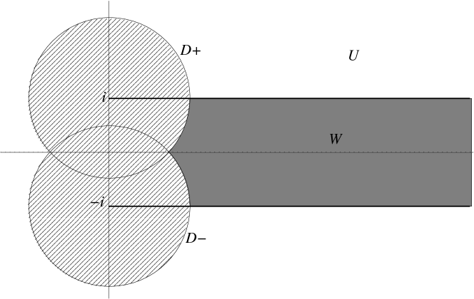
Figure 2: The subdomains $D_{+}$, $D_{-}$, $U$ and $W$.

First, let us estimate $\sup_{\mathbb{R}^{2}}|\mathcal{R}_{z}|$ for $z\in D_{+}$. As $z\to i$, we have $k_{+}(z)\to 0$ and $k_{-}(z)\to\sqrt{-2i}$. Thus, there exist positive constants $c_{0}\,$, $c_{1}$ and $c_{2}$ such that, for all $z\in D_{+}$,

$$|k_{+}(z)+k_{-}(z)|\geq\frac{1}{c_{0}}\,,\qquad|k_{+}(z)-k_{-}(z)|\leq c_{1}\,,\qquad|k_{-}(z)|\geq\frac{1}{c_{2}}\,.$$ (6.1)

According to (3.2), we then have, for all $(x,y)\in\mathbb{R}^{2}$ such that $xy\leq 0$,

$$|\mathcal{R}_{z}(x,y)|\leq\frac{1}{|k_{+}(z)+k_{-}(z)|}\leq c_{0}\,,$$ (6.2)

and, for all $(x,y)\in\big{\{}x\leq 0,y\leq 0\big{\}}$,

$$|\mathcal{R}_{z}(x,y)|\leq\frac{1}{2|k_{-}(z)|}\left(1+\frac{|k_{+}(z)-k_{-}(z)|}{|k_{+}(z)+k_{-}(z)|}\right)\leq\frac{c_{2}}{2}(1+c_{0}c_{1})\,.$$ (6.3)

It remains to check that there is no singularity as $z\rightarrow i$ for $x>0\,$, $y>0\,$:

$$|\mathcal{R}_{z}(x,y)| =\frac{1}{2|k_{+}(z)|}\left|e^{-k_{+}(z)|x-y|}+\Big{(}-1+\frac{2k_{+}(z)}{k_{+}(z)+k_{-}(z)}\Big{)}e^{-k_{+}(z)(|x|+|y|)}\right|$$

$$\leq\frac{1}{2|k_{+}(z)|}\left|e^{-k_{+}(z)|x-y|}-e^{-k_{+}(z)(|x|+|y|)}\right|+\frac{1}{|k_{+}(z)+k_{-}(z)|}$$

$$\leq c_{0}+\frac{1}{2|k_{+}(z)|}\left|\Big{(}e^{-k_{+}(z)|x-y|}-1\Big{)}-\Big{(}e^{-k_{+}(z)(|x|+|y|)}-1\Big{)}\right|$$

$$\leq c_{0}+\frac{|x-y|+|x|+|y|}{2}$$

$$\leq c_{0}+|x|+|y|\,,$$ (6.4)

where we have used the inequality $|e^{-\omega}-1|\leq|\omega|$ for ${\rm Re\,}\omega\geq 0$. Using (6.2), (6.3) and (6.4), we then get, for all $z\in D_{+}$,

$$\|K_{z}\|_{\mathrm{HS}}^{2} \leq\int_{\mathbb{R}^{2}}|V(x)|\Big{(}3c_{0}^{2}+\frac{c_{2}^{2}}{4}(1+c_{0}c_{1})^{2}+2\big{(}|x|+|y|\big{)}^{2}\Big{)}|V(y)|\,dx\,dy$$

$$\leq C_{+}\left(\int_{\mathbb{R}}(1+|x|^{2})|V(x)|\,dx\right)^{2}\,,$$ (6.5)

with some $C_{+}>0$.

Similarly, one can check that there exists $C_{-}>0$ such that, for all $z\in D_{-}$,

$$\|K_{z}\|_{\mathrm{HS}}^{2}\leq C_{-}\left(\int_{\mathbb{R}}(1+|x|^{2})|V(x)|\,dx\right)^{2}\,.$$ (6.6)

Now let us consider the region $U$. Notice that, as $|z|\rightarrow+\infty$, $z\in U$, we have

$$k_{+}(z)-k_{-}(z)\longrightarrow 0\qquad\mbox{and}\qquad k_{+}(z)\sim k_{-}(z)\sim\sqrt{-z}\,,$$

hence $|k_{+}+k_{-}|^{-1}$, $|k_{+}|^{-1}$, $|k_{-}|^{-1}$ and $|k_{+}-k_{-}|$ are uniformly bounded in $U$. Thus, there exists $C_{1}>0$ such that, for all $z\in U$,

$$\|K_{z}\|_{\mathrm{HS}}^{2}\leq\|V\|_{L^{1}(\mathbb{R})}^{2}\sup_{(x,y)\in\mathbb{R}^{2}}|\mathcal{R}_{z}(x,y)|^{2}\leq C_{1}\|V\|_{L^{1}(\mathbb{R})}^{2}\,.$$ (6.7)

Finally, for $z\in W$, we use the asymptotic expansions (4.2) and (4.4). In particular, there exist $c_{3}>0$, $c_{4}>0$ and $c_{5}>0$ such that, for all $z\in W$,

$$2|k_{\pm}(z)|\geq\frac{\sqrt{{\rm Re\,}z}}{c_{3}}\,,\quad|k_{-}(z)-k_{+}(z)|\leq c_{4}\sqrt{{\rm Re\,}z}\,,\quad|k_{+}(z)+k_{-}(z)|\geq\frac{1}{c_{5}\sqrt{{\rm Re\,}z}}\,.$$

Thus, according to (3.2), we have

$$\sup_{(x,y)\in\mathbb{R}^{2}}|\mathcal{R}_{z}(x,y)|\leq\frac{c_{3}}{\sqrt{{\rm Re\,}z}}+c_{3}c_{4}c_{5}\sqrt{{\rm Re\,}z}\leq\sqrt{C_{2}{\rm Re\,}z}$$

for some $C_{2}>0$, hence

$$\|K_{z}\|_{\mathrm{HS}}^{2}\leq C_{2}\,{\rm Re\,}z\,\|V\|_{L^{1}(\mathbb{R})}^{2}\,.$$ (6.8)

Gathering (6.5), (6.6), (6.7) and (6.8), we obtain, for all $z\in\mathbb{C}\setminus\big{(}\mathbb{R}_{+}+i\{-1,+1\}\big{)}$,

$$\|K_{z}\|_{\mathrm{HS}}^{2}\leq\max\Big{(}\max(C_{+},C_{-},C_{1})\big{\|}(1+|\cdot|^{2})V\big{\|}_{L^{1}(\mathbb{R})}^{2}\,,C_{2}\,{\rm Re\,}z\,\|V\|_{L^{1}(\mathbb{R})}^{2}\Big{)}\,,$$ (6.9)

and more precisely when $z\notin\mathcal{S}$,

$$\|K_{z}\|_{\mathrm{HS}}^{2}\leq\max(C_{+},C_{-},C_{1})\big{\|}(1+|\cdot|^{2})V\big{\|}_{L^{1}(\mathbb{R})}^{2}\,\,.$$

In particular, if $\|(1+|\cdot|^{2})V\|_{L^{1}(\mathbb{R})}^{2}<\max(C_{+},C_{-},C_{1})^{-1}$ and either $z\notin\mathcal{S}$ or ${\rm Re\,}z<(C_{2}\,\|V\|_{L^{1}(\mathbb{R})}^{2})^{-1}$, then $\|K_{z}\|_{\mathrm{HS}}<1$ and $-1$ cannot be in the spectrum of $K_{z}$. After the replacement $V\mapsto\varepsilon V$, we therefore get Theorem 2.3 as a consequence of Theorem 5.3. ∎

6.2 Proof of Theorem 2.4

Let $V$ satisfy the assumptions of Theorem 2.4 with $n\geq 2$ and $\varepsilon>0$. The present proof is again based on Theorem 5.3, but we use a more sophisticated estimate of the norm of $K_{z}$ for which the extra regularity hypotheses are needed.

The first step in our proof is to isolate the singular part of the kernel $\mathcal{K}_{z}$. The idea comes back to [32], where the singularity of the free resolvent $(-\Delta-z)^{-1}$ at $z=0$ is singled out. In the present setting, however, the resolvent $(H-z)^{-1}$ is rather singular as ${\rm Re\,}z\rightarrow+\infty$. In other words, we want to find a decomposition of the form

$$K_{z}=L_{z}+M_{z}\,,$$ (6.10)

where $\|L_{z}\|\to+\infty$ as ${\rm Re\,}z\to+\infty$, while $M_{z}$ stays uniformly bounded with respect to $z$. The integral kernels of $L_{z}$ and $M_{z}$ will be denoted by $\mathcal{L}_{z}$ and $\mathcal{M}_{z}$, respectively.

Notice that it is enough to consider $z\in\mathcal{S}$ since, according to Theorem 2.3, every eigenvalue of $H_{\varepsilon}$ belongs to the half-strip $\mathcal{S}$ provided that $\varepsilon$ is small enough.

In this paper, motivated by the asymptotic expansions (4.1), we use the decomposition (6.10) with the singular part $L_{z}$ given by the integral kernel

$$\mathcal{L}_{z}(x,y):=\sqrt{{\rm Re\,}z}\,|V|^{1/2}(x)\,e^{-i\sqrt{{\rm Re\,}z}\,(x+y)}\,V_{1/2}(y)\,.$$ (6.11)

Properties of $M_{z}$ are then stated in the following lemma.

Lemma 6.1.

For all $z\in\mathcal{S}$ and $(x,y)\in\mathbb{R}^{2}$, the integral kernel of the operator $M_{z}$ defined by (6.10) with (6.11) satisfies

$$\mathcal{M}_{z}(x,y)=\frac{1}{2}|V|^{1/2}(x)e^{-i\sqrt{{\rm Re\,}z}\,(x+y)}\big{[}{\rm Im\,}z\,(x+y)-(|x|+|y|)\big{]}V_{1/2}(y)+m_{z}(x,y)\,,$$ (6.12)

where for some $k>0\,$, the function $m_{z}$ satisfies, for all $z\in\mathcal{S}$ such that ${\rm Re\,}z\geq 1\,$,

$$|m_{z}(x,y)|\leq\frac{k}{\sqrt{{\rm Re\,}z}}\,|V|^{1/2}(x)\,(1+x^{2}+y^{2})\,|V|^{1/2}(y)\,.$$ (6.13)

If $V\in L^{1}\big{(}\mathbb{R},(1+x^{4})\,dx\big{)}$, then $\|M_{z}\|_{\mathrm{HS}}$ is uniformly bounded with respect to $z\in\mathcal{S}$.

Proof.

In the following computations we assume ${\rm Re\,}z\geq 1\,$.

First, let $x\geq 0$ and $y\leq 0$. Then, according to (3.2) and the asymptotic behaviour of $k_{+}(z)$ and $k_{-}(z)$ given in (4.1),

$$\mathcal{R}_{z}(x,y)=\frac{1}{k_{+}(z)+k_{-}(z)}\,e^{-k_{+}(z)\,x+k_{-}(z)\,y}=e^{-k_{+}(z)\,x+k_{-}(z)\,y}\big{(}\sqrt{{\rm Re\,}z}+\delta_{1}(z)\big{)}\,,$$

where $\delta_{1}(z)$ does not depend on $(x,y)$ and $\delta_{1}(z)=\mathcal{O}(1/\sqrt{{\rm Re\,}z})$. Thus,

$$\mathcal{M}_{z}(x,y)=\ \sqrt{{\rm Re\,}z}\,|V|^{1/2}(x)\,e^{-i\sqrt{{\rm Re\,}z}\,(x+y)}\left(e^{\Lambda_{z}(x,y)}-1\right)V_{1/2}(y)$$

$$+\delta_{1}(z)\,|V|^{1/2}(x)\,e^{-k_{+}(z)\,x+k_{-}(z)\,y}\,V_{1/2}(y)\,,$$ (6.14)

where

$$\Lambda_{z}(x,y):=\left(-k_{+}(z)+i\sqrt{{\rm Re\,}z}\right)x+\left(k_{-}(z)+i\sqrt{{\rm Re\,}z}\right)y\,.$$

Writing a Taylor expansion for the two real-valued functions

$$[0,1]\ni t\longmapsto{\rm Re\,}e^{t\Lambda_{z}(x,y)}\qquad\mbox{and}\qquad[0,1]\ni t\longmapsto{\rm Im\,}e^{t\Lambda_{z}(x,y)}\,,$$

we obtain that, for some $t_{1},t_{2}\in[0,1]$,

$$e^{\Lambda_{z}(x,y)}-1=\Lambda_{z}(x,y)+\frac{1}{2}\Big{[}{\rm Re\,}\big{(}\Lambda_{z}(x,y)^{2}e^{t_{1}\Lambda_{z}(x,y)}\big{)}+i\,{\rm Im\,}\big{(}\Lambda_{z}(x,y)^{2}e^{t_{2}\Lambda_{z}(x,y)}\big{)}\Big{]}\,.$$ (6.15)

Notice that, for all $z\in\mathcal{S}$, $x\geq 0$ and $y\leq 0$, ${\rm Re\,}\Lambda_{z}(x,y)\leq 0$, hence

$$\frac{1}{2}\Big{|}{\rm Re\,}\big{(}\Lambda_{z}(x,y)^{2}e^{t_{1}\Lambda_{z}(x,y)}\big{)}+i\,{\rm Im\,}\big{(}\Lambda_{z}(x,y)^{2}e^{t_{2}\Lambda_{z}(x,y)}\big{)}\Big{|}\leq|\Lambda_{z}(x,y)|^{2}\,.$$ (6.16)

Moreover, due to (4.1), we have

$$\Lambda_{z}(x,y)=\frac{({\rm Im\,}z-1)\,x+({\rm Im\,}z+1)\,y}{2\sqrt{{\rm Re\,}z}}+\frac{\beta_{z}\,x+\gamma_{z}\,y}{({\rm Re\,}z)^{3/2}}\,,$$

for some complex constants $\beta_{z}$ and $\gamma_{z}$ independent of $(x,y)$ and uniformly bounded with respect to $z$. As a consequence, (6.15) and (6.16) yield

$$e^{\Lambda_{z}(x,y)}-1=\frac{1}{\sqrt{{\rm Re\,}z}}\left(\frac{({\rm Im\,}z-1)\,x+({\rm Im\,}z+1)\,y}{2}+\delta_{2}(z;x,y)\right),$$

where, for all $z\in\mathcal{S}$, $x\geq 0$ and $y\leq 0$,

$$|\delta_{2}(z;x,y)|\leq C_{0}\,\frac{1+x^{2}+y^{2}}{\sqrt{{\rm Re\,}z}}\,,$$

with some $C_{0}>0$. Summing up, (6.14) reads

$$\mathcal{M}_{z}(x,y)=|V|^{1/2}(x)\left(\tilde{\mathcal{M}}_{z}^{0}(x,y)+r_{z}(x,y)\right)V_{1/2}(y)\,,$$ (6.17)

where ($x\geq 0$, $y\leq 0$)

$$\tilde{\mathcal{M}}_{z}^{0}(x,y):=\ \frac{1}{2}\,e^{-i\sqrt{{\rm Re\,}z}\,(x+y)}\,\big{[}({\rm Im\,}z-1)\,x+({\rm Im\,}z+1)\,y\big{]}$$

$$=\ \frac{1}{2}\,e^{-i\sqrt{{\rm Re\,}z}\,(x+y)}\,\big{[}{\rm Im\,}z\,(x+y)-(|x|+|y|)\big{]}$$ (6.18)

and

$$r_{z}(x,y):=e^{-i\sqrt{{\rm Re\,}z}\,(x+y)}\,\delta_{2}(z;x,y)+e^{-k_{+}(z)\,x+k_{-}(z)\,y}\,\delta_{1}(z)$$ (6.19)

satisfies, with some positive constant $C$,

$$\forall z\in\mathcal{S}\,,\ x\geq 0\,,\ y\leq 0\,,\quad|r_{z}(x,y)|\leq\frac{C}{\sqrt{{\rm Re\,}z}}\,(1+x^{2}+y^{2})\,.$$ (6.20)

By a similar analysis, we get the decomposition of the form (6.17) for $x\leq 0$ and $y\geq 0$ as well, where ($x\leq 0$, $y\geq 0$)

$$\tilde{\mathcal{M}}_{z}^{0}(x,y):=\ \frac{1}{2}e^{-i\sqrt{{\rm Re\,}z}\,(x+y)}\big{[}({\rm Im\,}z+1)\,x+({\rm Im\,}z-1)\,y\big{]}$$

$$=\ \frac{1}{2}e^{-i\sqrt{{\rm Re\,}z}\,(x+y)}\big{[}{\rm Im\,}z\,(x+y)-(|x|+|y|)\big{]}$$ (6.21)

and the bound (6.20) holds also for $x\leq 0$, $y\geq 0$.

The case $xy\geq 0$ can also be treated alike, by noticing that in this case the first term on the right-hand side of (3.2) satisfies

$$\left|\frac{1}{2k_{\pm}(z)}\,e^{-k_{\pm}(z)|x-y|}\right|\leq\frac{C^{\prime}}{\sqrt{{\rm Re\,}z}}$$

with some $C^{\prime}>0$. Moreover, using (4.1),

$$\pm\frac{k_{+}(z)-k_{-}(z)}{2k_{\pm}(z)\big{(}k_{+}(z)+k_{-}(z)\big{)}}\,e^{-k_{\pm}(z)(|x|+|y|)}-\sqrt{{\rm Re\,}z}\,e^{-i\sqrt{{\rm Re\,}z}\,(x+y)}\\ =\frac{1}{2}\,e^{-i\sqrt{{\rm Re\,}z}\,(x+y)}\,\big{[}{\rm Im\,}z\,(x+y)-(|x|+|y|)\big{]}+\rho_{z}(x,y)\,,$$

where $\rho_{z}(x,y)$ satisfies the bound (6.20). The decomposition (6.12) with (6.13) is therefore proved.

To complete the proof of the lemma, it remains to prove the uniform boundedness of $\mathcal{M}_{z}$. This can be deduced from (6.12) and (6.13). Indeed, with some $C_{1}>0$, we have, for ${\rm Re\,}z\geq 1$,

$$\|M_{z}\|_{\mathrm{HS}}^{2}\leq C_{1}\int_{\mathbb{R}^{2}}|V(x)|\,(1+x^{2}+y^{2})^{2}\,|V(y)|\,dx\,dy\,,$$

where the right hand side is finite if $V\in L^{1}(\mathbb{R},(1+x^{4})\,dx)$ and actually independent of $z$. If ${\rm Re\,}z\leq 1$, then according to (6.9) and the expression (6.11) of the kernel $\mathcal{L}_{z}$, we have

$$\|M_{z}\|_{\mathrm{HS}}\leq\|K_{z}\|_{\mathrm{HS}}+\|L_{z}\|_{\mathrm{HS}}\leq C_{2}\,\sqrt{\int_{\mathbb{R}^{2}}|V(x)|\,(1+|x|+|y|)^{2}\,|V(y)|\,dx\,dy}$$

with some $C_{2}>0$, hence the norm $\|M_{z}\|_{\mathrm{HS}}$ is uniformly bounded for ${\rm Re\,}z\leq 1$ as well. ∎

Remark 6.2.

Using a first-order expansion in (6.15) instead of the second-order expansion, we would obtain the uniform boundedness of $M_{z}$ under the weaker assumption $V\in L^{1}\big{(}\mathbb{R},(1+x^{2})\,dx)$. However, the second-order expansion in (6.15) is required in order to get the exact expression (6.18) of the principal term $\tilde{\mathcal{M}}_{z}^{0}(x,y)$ in (6.17).

Since $\|M_{z}\|$ is uniformly bounded with respect to $z\in\mathcal{S}$, the operator $(1+\varepsilon M_{z})$ is boundedly invertible for all $\varepsilon$ small enough. Consequently, in view of the identity

$$\varepsilon K_{z}+1=\varepsilon(L_{z}+M_{z})+1=(1+\varepsilon M_{z})\big{[}\varepsilon(1+\varepsilon M_{z})^{-1}L_{z}+1\big{]}$$

and Theorem 5.3, we have (for all $z\in\mathcal{S}$)

$$z\in\sigma_{\mathrm{p}}(H_{\varepsilon})\quad\Longleftrightarrow\quad-1\in\sigma\big{(}\varepsilon(1+\varepsilon M_{z})^{-1}L_{z}\big{)}\,.$$ (6.22)

From the definition (6.11) we see that $L_{z}$ is a rank-one operator. Consequently, $\varepsilon(1+\varepsilon M_{z})^{-1}L_{z}$ is of rank one too. Indeed, for all $f\in L^{2}(\mathbb{R})$, we have

$$\varepsilon(1+\varepsilon M_{z})^{-1}L_{z}f=\varepsilon\sqrt{{\rm Re\,}z}\,(f,\bar{\psi}_{z})\,(1+\varepsilon M_{z})^{-1}\phi_{z}\,,$$

where

$$\phi_{z}(x):=e^{-i\sqrt{{\rm Re\,}z}\,x}\,|V|^{1/2}(x)\qquad\mbox{and}\qquad\psi_{z}(x):=e^{-i\sqrt{{\rm Re\,}z}\,x}\,V_{1/2}(x)\,.$$

It follows that $\varepsilon(1+\varepsilon M_{z})^{-1}L_{z}$ has the unique non-zero eigenvalue

$$\varepsilon\sqrt{{\rm Re\,}z}\,\left((1+\varepsilon M_{z})^{-1}\phi_{z},\bar{\psi}_{z}\right).$$

Equivalence (6.22) thus reads

$$z\in\sigma_{\mathrm{p}}(H_{\varepsilon})\quad\Longleftrightarrow\quad-1=\varepsilon\sqrt{{\rm Re\,}z}\,\left((1+\varepsilon M_{z})^{-1}\phi_{z},\bar{\psi}_{z}\right)\,.$$ (6.23)

Note that the right hand side represents an implicit equation for $z$.

Writing

$$(1+\varepsilon M_{z})^{-1}=\sum_{j=0}^{n-1}(-1)^{j}\varepsilon^{j}M_{z}^{j}+(-1)^{n}\varepsilon^{n}M_{z}^{n}(1+\varepsilon M_{z})^{-1}\,,$$

the condition on the right hand side of (6.23) reads

$$\frac{1}{\sqrt{{\rm Re\,}z}}=\sum_{j=1}^{n}(-1)^{j}\left(M_{z}^{j-1}\phi_{z},\bar{\psi}_{z}\right)\varepsilon^{j}+(-1)^{n+1}\left(M_{z}^{n}(1+\varepsilon M_{z})^{-1}\phi_{z},\bar{\psi}_{z}\right)\varepsilon^{n+1}\,.$$ (6.24)

In the following we estimate each term on the right hand side of (6.24).

For $j=1,\dots,n\,$, denoting

$$V^{\otimes j}(x_{1},\dots,x_{j}):=V(x_{1})\dots V(x_{j})\,,$$

and using the decomposition (6.14) with (6.21), we have

$$\left(M_{z}^{j-1}\phi_{z},\bar{\psi}_{z}\right)=\ \int_{\mathbb{R}^{j}}\mathcal{M}_{z}(x_{1},x_{2})\dots\mathcal{M}_{z}(x_{j-1},x_{j})\,\phi_{z}(x_{j})\,\psi_{z}(x_{1})\,dx_{1}\dots dx_{j}$$

$$=\ \int_{\mathbb{R}^{j}}\left(\prod_{\ell=1}^{j-1}|V|^{1/2}(x_{\ell})\big{[}\tilde{\mathcal{M}}_{z}^{0}(x_{\ell},x_{\ell+1})+r_{z}(x_{\ell},x_{\ell+1})\big{]}V_{1/2}(x_{\ell+1})\right)$$

$$\times|V|^{1/2}(x_{j})\,e^{-i\sqrt{{\rm Re\,}z}\,(x_{1}+x_{j})}\,V_{1/2}(x_{1})\,dx_{1}\dots dx_{j}$$

$$=\ \int_{\mathbb{R}^{j}}e^{-i\sqrt{{\rm Re\,}z}\,(x_{1}+x_{j})}\,V^{\otimes j}(x_{1},\dots,x_{j})$$

$$\times\prod_{\ell=1}^{j-1}\big{[}\tilde{\mathcal{M}}_{z}^{0}(x_{\ell},x_{\ell+1})+r_{z}(x_{\ell},x_{\ell+1})\big{]}dx_{1}\dots dx_{j}$$

$$=\ I_{j-1}(z)+R_{j-1}(z)\,,$$ (6.25)

where

$$I_{j-1}(z):=\frac{1}{2^{j-1}}\int_{\mathbb{R}^{j}}e^{-2i\sqrt{{\rm Re\,}z}\,\sum_{\ell=1}^{j}x_{\ell}}\,V^{\otimes j}(x_{1},\dots,x_{j})\\ \times\prod_{\ell=1}^{j-1}\big{[}{\rm Im\,}z\,(x_{\ell}+x_{\ell+1})-(|x_{\ell}|+|x_{\ell+1}|)\big{]}dx_{1}\dots dx_{j}$$ (6.26)

and $R_{j-1}(z):=(M_{z}^{j-1}\phi_{z},\bar{\psi}_{z})-I_{j-1}(z)$ contains all the integral terms involving at least one factor of the form $r_{z}(x_{\ell},x_{\ell+1})$. Using (6.20), one can easily check that

$$R_{j-1}(z)=\mathcal{O}\left(\frac{1}{\sqrt{{\rm Re\,}z}}\right)$$ (6.27)

whenever $V\in L^{1}(\mathbb{R},(1+x^{2n})\,dx)$.

On the other hand, we have

$$\prod_{\ell=1}^{j-1}\big{[}{\rm Im\,}z\,(x_{\ell}+x_{\ell+1})-(|x_{\ell}|+|x_{\ell+1}|)\big{]}=\sum_{\vec{\ell}\in\mathcal{J}_{j-1}}\prod_{m=1}^{j-1}({\rm Im\,}z\,x_{\ell_{m}}-|x_{\ell_{m}}|)\,,$$

for a subset $\mathcal{J}_{j-1}\subset\{1,\dots,j\}^{j-1}$ such that, for all $\vec{\ell}\in\mathcal{J}_{j-1}$, each coordinate in $\vec{\ell}$ is repeated at most twice. Consequently, separating the variables in (6.26), we get, for some positive integer $M_{j}$,

$$I_{j-1}(z)=\frac{1}{2^{j-1}}\sum_{k=1}^{M_{j}}I_{j-1}^{(k)}(z)\,,$$ (6.28)

where each term $I_{j-1}^{(k)}(z)$ has the form

$$I_{j-1}^{(k)}(z) = \left(\int_{\mathbb{R}}e^{-2i\sqrt{{\rm Re\,}z}\,x}\,V(x)\,dx\right)^{a_{k,j}}$$

$$\times\left(\int_{\mathbb{R}}e^{-2i\sqrt{{\rm Re\,}z}\,x}({\rm Im\,}z\,x-|x|)\,V(x)\,dx\right)^{b_{k,j}}$$

$$\times\left(\int_{\mathbb{R}}e^{-2i\sqrt{{\rm Re\,}z}\,x}\,({\rm Im\,}z\,x-|x|)^{2}V(x)\,dx\right)^{c_{k,j}}\,,$$

with $a_{k,j},b_{k,j},c_{k,j}$ such that

$$\left\{\begin{array}[]{l}a_{k,j}>0\,,\ b_{k,j}\geq 0\,,\ c_{k,j}\geq 0\,,\\ a_{k,j}+b_{k,j}+c_{k,j}=j\,,\\ b_{k,j}+2c_{k,j}=j-1\,.\end{array}\right.$$

Thus, if $\mathcal{F}[f](\xi)$ denotes the Fourier transform of $f$ at point $\xi$, we have

$$I_{j-1}^{(k)}(z) = \left(\mathcal{F}[V](2\sqrt{{\rm Re\,}z})\right)^{a_{k,j}}\left(\mathcal{F}\big{[}({\rm Im\,}z\,x-|x|)V(x)\big{]}(2\sqrt{{\rm Re\,}z})\right)^{b_{k,j}}$$ (6.29)

$$\times\left(\mathcal{F}\big{[}({\rm Im\,}z\,x-|x|)^{2}V(x)\big{]}(2\sqrt{{\rm Re\,}z})\right)^{c_{k,j}}\,.$$

Now, since for $s=1,2$ the function $x\mapsto({\rm Im\,}z\,x-|x|)^{s}V(x)$ belongs to $L^{1}(\mathbb{R})$ by assumption, its Fourier transform is in $L^{\infty}(\mathbb{R})$ and it is continuous. Hence there exists $M_{1}>0$ such that, for all $z\in\mathcal{S}$ and $s=1,2$,

$$\left|\mathcal{F}\big{[}({\rm Im\,}z\,x-|x|)^{s}V(x)\big{]}(2\sqrt{{\rm Re\,}z})\right|\leq M_{1}\,.$$

Similarly, since $V\in W^{1,1}(\mathbb{R})$, the function $\xi\mapsto\xi\,\mathcal{F}[V](\xi)$ belongs to $L^{\infty}(\mathbb{R})$ and it is continuous. Hence there exists $M_{2}>0$ such that, for all $z\in\mathcal{S}$,

$$\left|\mathcal{F}[V](2\sqrt{{\rm Re\,}z})\right|\leq\frac{M_{2}}{\sqrt{{\rm Re\,}z}}\,.$$

Thus (6.28) and (6.29) give

$$I_{j-1}(z)=\mathcal{O}\left(\frac{1}{\sqrt{{\rm Re\,}z}}\right)\,.$$ (6.30)

Finally, (6.25), (6.27) and (6.30) yield

$$\left(M_{z}^{j-1}\phi_{z},\bar{\psi}_{z}\right)=\mathcal{O}\left(\frac{1}{\sqrt{{\rm Re\,}z}}\right)$$

for all $j=1,\dots,n$. Thus, according to (6.24),

$$\frac{1}{\sqrt{{\rm Re\,}z}}\,\big{(}1-\mathcal{O}(\varepsilon)\big{)}=(-1)^{n+1}\left(M_{z}^{n}(1+\varepsilon M_{z})^{-1}\phi_{z},\bar{\psi}_{z}\right)\varepsilon^{n+1}\,,$$

uniformly with respect to $z$ as $\varepsilon\rightarrow 0$. We then notice that the right hand side in the above identity has the form $\mathcal{O}(\varepsilon^{n+1})$, uniformly with respect to $z$, as $\varepsilon\rightarrow 0$. Therefore, we have

$$\frac{1}{\sqrt{{\rm Re\,}z}}=\mathcal{O}(\varepsilon^{n+1})\,,$$

which concludes the proof of Theorem 2.4. ∎

7 Examples

7.1 Dirac interaction

In order to test our results on an explicitly solvable model, let us consider the operator formally given by the expression

$$H_{\alpha}=-\frac{d^{2}}{dx^{2}}+i\mathop{\mathrm{sgn}}\nolimits(x)+\alpha\,\delta(x)\,,\qquad\alpha\in\mathbb{C}\,,$$

where $\delta$ is the Dirac delta function. In fact, $H_{\alpha}$ can be rigorously defined (cf. [20, Ex. 5.27]) as the m-sectorial operator in $L^{2}(\mathbb{R})$ associated with the form sum $h+\alpha v$, where

$$v(\psi,\phi):=\psi(0)\bar{\phi}(0)\,,\qquad\mathsf{Dom}(v):=W^{1,2}(\mathbb{R})\,.$$

We have

$$(H_{\alpha}\psi)(x) =-\psi^{\prime\prime}(x)+i\mathop{\mathrm{sgn}}\nolimits(x)\,\psi(x)\quad\mbox{for a.e. }x\in\mathbb{R}\,,$$

$$\mathsf{Dom}(H_{\alpha}) =\left\{\psi\in W^{1,2}(\mathbb{R})\cap W^{2,2}(\mathbb{R}\setminus\{0\}):\ \psi^{\prime}(0^{+})-\psi^{\prime}(0^{-})=\alpha\,\psi(0)\right\}\,.$$

It is also possible to show that $H_{\alpha}$ is $\mathcal{T}$-self-adjoint.

Using for instance [12, Corol. IX.4.2], we have the stability result

$$\sigma_{\mathrm{ess}}(H_{\alpha})=\sigma_{\mathrm{ess}}(H)=[0,+\infty)+i\,\{-1,+1\}$$

for all $\alpha\in\mathbb{C}$. Since $H_{\alpha}$ is $\mathcal{T}$-self-adjoint, the residual spectrum of $H_{\alpha}$ is empty (cf. [20, Sec. 5.2.5.4]). Finally, the eigenvalue problem for $H_{\alpha}$ can be solved explicitly and we find that $H_{\alpha}$ possesses a unique (discrete) eigenvalue given by

$$\lambda(\alpha):=\frac{1}{\alpha^{2}}-\frac{\alpha^{2}}{4}$$ (7.1)

if, and only if,

$$\lambda(\alpha)\not\in[0,+\infty)+i\,\{-1,+1\}\,.$$ (7.2)

In particular, the eigenvalue exists for all $\alpha\in\mathbb{R}\setminus\{0\}$ and in this case it is real. It is interesting that the rate at which $\lambda(\alpha)$ tends to infinity as $\alpha\to 0$ coincides with the bound of Theorem 2.3, even if this theorem does not apply to the present singular potential and even for non-real $\alpha$.

Now, in order to state the condition (7.2) more explicitly in terms of $\alpha$, let us set, for all $\sigma=(\sigma_{1},\sigma_{2},\sigma_{3})\in\{-1,+1\}^{3}$,

$$\Gamma_{\sigma}:=\left\{\sigma_{1}\sqrt{-2(r+i\sigma_{2})+2\sigma_{3}\sqrt{r(r+2i\sigma_{2})}}\,:\ r\in[0,+\infty)\right\}\,.$$

Notice that, for all $r\in[0,+\infty)$, the square roots in the expression above are well defined. Then the condition (7.2) is equivalent to $\alpha\notin\Gamma$, where

$$\Gamma:=\bigcup_{\sigma\in\{-1,+1\}^{3}}\Gamma_{\sigma}\,.$$ (7.3)

The curve $\Gamma$ is represented in Figure 3.

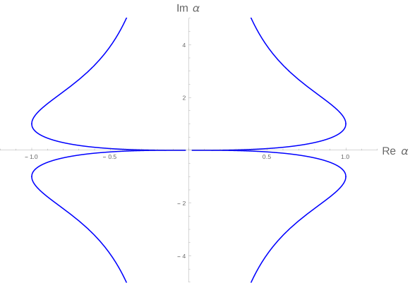
Figure 3: The curve $\Gamma$ in the complex plane representing values of $\alpha$ for which the eigenvalue of $H_{\alpha}$ does not exist.

Let us summarise the spectral properties into the following proposition.

Proposition 7.1.

For any $\alpha\in\mathbb{C}$, we have

$$\sigma_{\mathrm{r}}(H_{\alpha}) =\varnothing\,,$$

$$\sigma_{\mathrm{c}}(H_{\alpha}) =[0,+\infty)+i\,\{-1,+1\}\,,$$

$$\sigma_{\mathrm{p}}(H_{\alpha}) =\begin{cases}\varnothing&\mbox{if}\quad\alpha\in\Gamma\,,\\ \{\lambda(\alpha)\}&\mbox{if}\quad\alpha\not\in\Gamma\,,\end{cases}$$

where $\lambda(\alpha)$ is given by (7.1) and $\Gamma$ is the domain defined in (7.3).

7.2 Step-like potential

To have a definitive support for the existence of discrete spectra for the operators of the type (2.6), here we consider $\varepsilon=1$ and the following step-like profile for the perturbing potential:

$$V_{a,b}(x):=\left(-i\,\mathop{\mathrm{sgn}}\nolimits(x)-b\right)\chi_{[-a,a]}(x)\,,$$

where $a>0$ and $b\in\mathbb{C}$. We set $H_{a,b}:=H+V_{a,b}$. By Proposition 5.5,

$$\sigma_{\mathrm{ess}}(H_{a,b})=[0,+\infty)+i\,\{-1,+1\}$$ (7.4)

for all $a>0$ and $b\in\mathbb{C}$.

The differential equation of the eigenvalue problem $H_{a,b}\psi=\lambda\psi$ can be solved in terms of sines and cosines in each of the intervals $(-\infty,-a)$, $(-a,a)$ and $(a,+\infty)$. Choosing integrable solutions in the infinite intervals and gluing the respective solutions at $\pm a$ by requiring the $W^{2,2}$-regularity, we arrive at the following equation

$$\big{[}\sqrt{\lambda^{2}+1}-\lambda-b\big{]}\frac{\sin\big{(}2a\sqrt{\lambda+b}\big{)}}{\sqrt{\lambda+b}}-i\big{(}\sqrt{\lambda+i}-\sqrt{\lambda-i}\big{)}\,\cos\big{(}2a\sqrt{\lambda+b}\big{)}=0$$ (7.5)

for eigenvalues $\lambda$ satisfying $|{\rm Im\,}\lambda|<1$ and $\lambda+b\not\in(-\infty,0)$. The equation for the case $\lambda=-b$ is recovered after taking the limit $\lambda\to-b$ in the above equation. For eigenvalues $\lambda$ satisfying $|{\rm Im\,}\lambda|<1$ and $\lambda+b\in(-\infty,0)$, we find

$$\big{[}\sqrt{\lambda^{2}+1}-\lambda-b\big{]}\frac{\sinh\big{(}2a\sqrt{|\lambda+b|}\big{)}}{\sqrt{|\lambda+b|}}-i\big{(}\sqrt{\lambda+i}-\sqrt{\lambda-i}\big{)}\,\cosh\big{(}2a\sqrt{|\lambda+b|}\big{)}=0\,.$$

In the same manner, it is possible to derive equations for eigenvalues $\lambda$ satisfying $|{\rm Im\,}\lambda|\geq 1$. However, we shall not present these formulae, for below we are particularly interested in real eigenvalues. We only mention that it is easy to verify that no point in the essential spectrum (7.4) can be an eigenvalue.

Henceforth, we investigate the existence of real eigenvalues. Moreover, we restrict to real $b$ and look for eigenvalues $\lambda>-b$, so that it is enough to work with (7.5). First of all, notice that, for any $\lambda>-b$ satisfying (7.5), $\sin\big{(}2a\sqrt{\lambda+b}\big{)}$ never vanishes. At the same time, ${\rm Im\,}\sqrt{\lambda+i}$ is non-zero for real $\lambda$. We can thus rewrite (7.5) as follows

$$\cot\big{(}2a\sqrt{\lambda+b}\big{)}=-\frac{\sqrt{\lambda^{2}+1}-(\lambda+b)}{2\,\sqrt{\lambda+b}\ {\rm Im\,}\sqrt{\lambda+i}}\sim b\qquad\mbox{as}\quad\lambda\to+\infty\,.$$

Since there is a periodic function with range $\mathbb{R}$ on the left hand side, it follows from the asymptotics that $H_{a,b}$ possesses infinitely many eigenvalues for every real $b$. Let us highlight this result by the following proposition.

Proposition 7.2.

For any $a>0$ and $b\in\mathbb{R}$, $H_{a,b}$ possesses infinitely many distinct real discrete eigenvalues.

Several real eigenvalues of $H_{a,b}$ as functions of $b\in\mathbb{R}$ are represented in Figure 4.

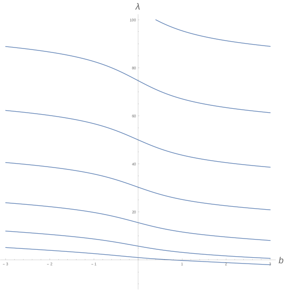
Figure 4: Dependence of real eigenvalues of $H_{a,b}$ on $b$ for $a=1$.

7.3 Dirichlet realisation

Since the spectrum of $H$ is the union of the two half-lines $\mathbb{R}_{+}+i$ and $\mathbb{R}_{+}-i$, one might have expected the operator $H$ to behave as some sort of decoupling of two operators $-\frac{d^{2}}{dx^{2}}+i$ in $L^{2}(\mathbb{R}_{+})$ and $-\frac{d^{2}}{dx^{2}}-i$ in $L^{2}(\mathbb{R}_{-})$. The existence of non-trivial pseudospectra (cf. Theorem 2.2) actually indicates that this is not the case. Indeed, the situation strongly depends on the way the operator is defined, emphasising the importance of the choice of domain in the pseudospectral behaviour of an operator.

For comparison, let $H^{D}$ be the operator in $L^{2}(\mathbb{R})$ that acts as $H$ in $\mathbb{R}_{+}^{*}:=(0,+\infty)$ and $\mathbb{R}_{-}^{*}:=(-\infty,0)$, but satisfies an extra Dirichlet condition at zero, i.e.,

$$\mathsf{Dom}(H^{D}):=\big{(}W^{2,2}\cap W_{0}^{1,2}\big{)}\big{(}\mathbb{R}\setminus\{0\}\big{)}\,.$$

Considering this operator instead of $H$ means that the previous matching conditions at $x=0$, $u(0^{-})=u(0^{+})$ and $u^{\prime}(0^{-})=u^{\prime}(0^{+})$ for $u\in\mathsf{Dom}(H)$, are replaced by the conditions $u(0^{-})=0=u(0^{+})$ for $u\in\mathsf{Dom}(H^{D})$.

We can write $H^{D}$ as a direct sum

$$H^{D}=H^{D}_{-}\oplus H^{D}_{+}\,,$$ (7.6)

where $H^{D}_{\pm}$ are operators in $L^{2}(\mathbb{R}_{\pm}^{*})$ defined by

$$H^{D}_{\pm}:=-\frac{d^{2}}{dx^{2}}\pm i\,,\qquad\mathsf{Dom}(H^{D}_{\pm}):=\big{(}W^{2,2}\cap W_{0}^{1,2}\big{)}(\mathbb{R}_{\pm}^{*})\,.$$ (7.7)

Since the spectra of $H^{D}_{\pm}$ are trivially found, we therefore have (see [12, Sec. IX.5])

$$\sigma(H^{D})=\sigma(H^{D}_{-})\cup\sigma(H^{D}_{+})=\mathbb{R}_{+}+i\,\{-1,+1\}\,.$$

Hence $H^{D}$ and $H$ have the same spectrum (cf. Proposition 2.1).

We can also decompose the resolvent of $H_{D}$ as follows

$$(H^{D}-z)^{-1}=(H^{D}_{-}-z)^{-1}\oplus(H^{D}_{+}-z)^{-1}$$

for every $z\not\in\mathbb{R}_{+}+i\,\{-1,+1\}$. Since $H^{D}_{\pm}$ are obtained from self-adjoint operators shifted by a constant, they both have trivial pseudospectra. Consequently, $H^{D}$ has trivial pseudospectra as well. In other words, although $H^{D}$ and $H$ have the same spectrum, that of $H$ is far more unstable (cf. Theorem 2.2).

To be more specific, let us write down the integral kernel $\mathcal{R}_{z}^{D}$ of $(H^{D}-z)^{-1}$. For $f\in L^{2}(\mathbb{R})$, the function $(H^{D}-z)^{-1}f$ has the form (3.4), where the constants $A_{+},A_{-},B_{+},B_{-}$ are uniquely determined by the Dirichlet condition at $0$ together with the condition $(H^{D}-z)^{-1}f(x)\to 0$ as $x\to\pm\infty$. The former yields $B_{+}=-A_{+}$ and $B_{-}=-A_{-}$, while the latter gives the following values for $A_{+}$ and $A_{-}$:

$$A_{+}=\frac{1}{2k_{+}(z)}\int_{0}^{+\infty}f(y)\,e^{-k_{+}(z)y}\,dy\,,\qquad A_{-}=-\frac{1}{2k_{-}(z)}\int_{-\infty}^{0}f(y)\,e^{k_{+}(z)y}\,dy\,.$$

Eventually, we obtain the following expression for the integral kernel:

$$\mathcal{R}_{z}^{D}(x,y)=\frac{1}{2k_{\pm}(z)}\left(e^{-k_{\pm}(z)|x-y|}-e^{-k_{\pm}(z)(|x|+|y|)}\right)\chi_{\mathbb{R}_{\pm}}(y)\,,\qquad\pm x>0\,.$$

Now, as in Section 5.1, we can consider the perturbed operator

$$H_{\varepsilon}^{D}:=H^{D}\dot{+}\varepsilon V$$

for any $V\in L^{1}(\mathbb{R})$. We claim that, under the additional assumption $V\in L^{1}(\mathbb{R},(1+x^{2})\,dx)$, the Hilbert-Schmidt norm of the Birman-Schwinger operator

$$K_{z}^{D}:=|V|^{1/2}\,(H^{D}-z)^{-1}\,V_{1/2}$$

is uniformly bounded with respect to $z\notin\mathbb{R}^{+}+i\{-1,1\}$. To see it, let us first assume $x>0$. If $|z-i|\leq c_{0}$ for some positive $c_{0}$, then

$$|\mathcal{R}_{z}^{D}(x,y)| \leq\frac{1}{2|k_{+}(z)|}\left(\big{|}e^{-k_{+}(z)|x-y|}-1\big{|}+\big{|}(e^{-k_{+}(z)(|x|+|y|)}-1\big{|}\right)$$

$$\leq\frac{|x-y|+|x|+|y|}{2}\,,$$

where we have used the inequality $|e^{-\omega}-1|\leq|\omega|$ for ${\rm Re\,}\omega\geq 0$. On the other hand, if $|z-i|>c_{0}$, then $|k_{+}(z)|$ is uniformly bounded from below, hence $\mathcal{R}_{z}^{D}(x,y)$ is uniformly bounded with respect to $x\geq 0$, $y\in\mathbb{R}$ and $z$ such that $|z-i|>c_{0}$. The same analysis can be performed for $x<0$, thus there exists $C>0$ such that, for all $(x,y)\in\mathbb{R}^{2}$ and $z\notin[0,+\infty)+i\{-1,1\}$,

$$|\mathcal{R}_{z}^{D}(x,y)|\leq C(1+|x|+|y|)\,.$$

Consequently, the computation of the Hilbert-Schmidt norm of $K_{z}^{D}$ yields

$$\|K_{z}^{D}\|_{\mathrm{HS}}\leq C\int_{\mathbb{R}}(1+x^{2})|V(x)|\,dx\,.$$ (7.8)

After noticing that $\sigma_{\mathrm{ess}}(H^{D}_{\varepsilon})=\sigma_{\mathrm{ess}}(H^{D})$ for all $\varepsilon\in\mathbb{R}$ (by the same arguments as in the proof of Proposition 5.5), the Birman-Schwinger principle (i.e. a version of Theorem 5.3 for $H^{D}_{\varepsilon}$) leads to the following statement.

Proposition 7.3.

Let $V\in L^{1}\left(\mathbb{R},(1+x^{2})\,dx\right)$. There exists a positive constant $\varepsilon_{0}>0$ such that, for all $\varepsilon\in(0,\varepsilon_{0})$, we have

$$\sigma(H^{D}_{\varepsilon})=\sigma(H^{D})=\mathbb{R}_{+}+i\,\{-1,1\}\,.$$

In other words, in the simpler situation of the operator $H^{D}$, we are able to prove the absence of weakly coupled eigenvalues. Proposition 7.3 can be considered as some sort of “Hardy inequality” or “absence of virtual bound state” for the non-self-adjoint operator $H^{D}$. Let us also notice that a similar result has been established by Frank [13] in the case of Schrödinger operators with complex potentials in three and higher dimensions.

Acknowledgment

The authors are grateful to Mark Embree for his Figure 1 and to Petr Siegl for valuable suggestions. The authors also thank the anonymous referee for helpful comments. The research was partially supported by the project RVO61389005 and the GACR grant No. 14-06818S. The first author acknowledges the support of the ANR project NOSEVOL. The second author also acknowledges the award from the Neuron fund for support of science, Czech Republic, May 2014.

References

- [1] A. A. Abramov, A. Aslanyan, and E. B. Davies, Bounds on complex eigenvalues and resonances, J. Phys. A: Math. Gen. 34 (2001), 57–72.
- [2] M. Sh. Birman, On the spectrum of singular boundary-value problems, Mat. Sb. 55 (1961), 127–174, (in Russian). English translation in: Eleven Papers on Analysis, AMS Transl. 53, 23-80, AMS, Providence, R.I., 1966.
- [3] R. Blackenbecler, M. L. Goldberger, and B. Simon, The bound states of weakly coupled long-range one-dimensional quantum Hamiltonians, Ann. Phys. 108 (1977), 69–78.
- [4] D. Borisov and D. Krejčiřík, -symmetric waveguides, Integ. Equ. Oper. Theory 62 (2008), 489–515.
- [5] D. C. Brody and E.-M. Graefe, Mixed-state evolution in the presence of gain and loss, Phys. Rev. Lett. 109 (2012), 230405.
- [6] V. Bruneau and E. M. Ouhabaz, Lieb-Thirring estimates for non self-adjoint Schrödinger operators, J. Math. Phys. 49 (2008), 093504.
- [7] E. B. Davies, Semi-classical states for non-self-adjoint Schrödinger operators, Comm. Math. Phys. 200 (1999), 35–41.
- [8] , Linear operators and their spectra, Cambridge University Press, 2007.
- [9] M. Demuth, M. Hansmann, and G. Katriel, On the discrete spectrum of non-selfadjoint operators, J. Funct. Anal. 257 (2009), 2742–2759.
- [10] , Lieb-Thirring type inequalities for Schrödinger operators with a complex-valued potential, Integ. Equ. Oper. Theory 75 (2013), 1–5.
- [11] N. Dencker, J. Sjöstrand, and M. Zworski, Pseudospectra of semiclassical (pseudo-) differential operators, Comm. Pure Appl. Math. 57 (2004), 384–415.
- [12] D. E. Edmunds and W. D. Evans, Spectral theory and differential operators, Oxford University Press, Oxford, 1987.
- [13] R. L. Frank, Eigenvalue bounds for Schrödinger operators with complex potentials, Bull. Lond. Math. Soc. 43 (2011), 745–750.
- [14] R. L. Frank, A. Laptev, E. H. Lieb, and R. Seiringer, Lieb-Thirring inequalities for Schrödinger operators with complex-valued potentials, Lett. Math. Phys. 77 (2006), 309–316.
- [15] R. Henry, Spectral instability for the complex Airy operator and even non-selfadjoint anharmonic oscillators, J. Spectr. Theory 4 (2014), 349–364.
- [16] , Spectral projections of the complex cubic oscillator, Ann. H. Poincaré 15 (2014), 2025–2043.
- [17] M. Hitrik, J. Sjöstrand, and J. Viola, Resolvent estimates for elliptic quadratic differential operators, Anal. PDE 6 (2013), 181–196.
- [18] T. Kato, Perturbation theory for linear operators, Springer-Verlag, Berlin, 1966.
- [19] M. Klaus, On the bound state of Schrödinger operators in one dimension, Ann. Phys. 108 (1977), 288–300.
- [20] D. Krejčiřík and P. Siegl, Elements of spectral theory without the spectral theorem, In Non-selfadjoint operators in quantum physics: Mathematical aspects (432 pages), F. Bagarello, J.-P. Gazeau, F. H. Szafraniec, and M. Znojil, Eds., Wiley-Interscience, 2015.
- [21] D. Krejčiřík, P. Siegl, M. Tater, and J. Viola, Pseudospectra in non-Hermitian quantum mechanics, arXiv:1402.1082 [math-SP] (2014).
- [22] A. Laptev and O. Safronov, Eigenvalue estimates for Schrödinger operators with complex potentials, Comm. Math. Phys. 292 (2009), 29–54.
- [23] S. Longhi, Bloch Oscillations in Complex Crystals with Symmetry, Phys. Rev. Lett. 103 (2009), 123601.
- [24] B. Mityagin, P. Siegl, and J. Viola, Differential operators admitting various rates of spectral projection growth, arXiv:1309.3751 (2013).
- [25] R. Novák, Bound states in waveguides with complex Robin boundary conditions, Asympt. Anal., to appear.
- [26] , On the pseudospectrum of the harmonic oscillator with imaginary cubic potential, Int. J. Theor. Phys., to appear.
- [27] K. Pravda-Starov, On the pseudospectrum of elliptic quadratic differential operators, Duke Math. J. 145 (2008), 249–279.
- [28] J. S. Schwinger, On the bound states of a given potential, Proc. Natl. Acad. Sci. U.S.A. 47 (1961), 122–129.
- [29] P. Siegl, -Symmetric Square Well-Perturbations and the Existence of Metric Operator, Int. J. Theor. Phys. 50 (2011), 991–996.
- [30] P. Siegl and D. Krejčiřík, On the metric operator for the imaginary cubic oscillator, Phys. Rev. D 86 (2012), 121702(R).
- [31] B. Simon, Quantum mechanics for Hamiltonians defined by quadratic forms, Princeton Univ. Press., New Jersey, 1971.
- [32] , The bound state of weakly coupled Schrödinger operators in one and two dimensions, Ann. Phys. 97 (1976), 279–288.
- [33] L. N. Trefethen and M. Embree, Spectra and pseudospectra, Princeton University Press, 2005.
- [34] J. Viola, Spectral projections and resolvent bounds for partially elliptic quadratic differential operators, J. Pseudo-Differ. Oper. Appl. 4 (2013), 145–221.
- [35] T. Weidl, Remarks on virtual bound states for semi-bounded operators, Commun. in Partial Differential Equations 24 (1999), 25–60.
- [36] T. G. Wright, EigTool, 2002, Software available at https://github.com/eigtool.
- [37] M. Znojil, -symmetric square well, Phys. Lett. A 285 (2001), 7–10.
- [38] M. Znojil and G. Lévai, Spontaneous breakdown of -symmetry in the solvable square-well model, Mod. Phys. Lett. A 16 (2001), 2273–2280.
- [39] M. Zworski, A remark on a paper of E. B. Davies, Proc. Amer. Math. Soc. 129 (2001), 2955–2957.