Methane on Uranus: The case for a compact CH₄ cloud layer at low latitudes and a severe CH₄ depletion at high-latitudes based on re-analysis of Voyager occultation measurements and STIS spectroscopy

Abstract

Lindal et al. (1987, J. Geophys. Res. 92, 14987-15001) presented a range of temperature and methane profiles for Uranus that were consistent with 1986 Voyager radio occultation measurements of refractivity versus altitude. A localized refractivity slope variation near 1.2 bars was interpreted to be the result of a condensed methane cloud layer. However, models fit to near-IR spectra found particle concentrations much deeper in the atmosphere, in the 1.5-3 bar range (Sromovsky et al. 2006, Icarus 182, 577-593, Sromovsky and Fry 2008, Icarus 193, 211-229, Irwin et al. 2010, Icarus 208, 913-926), and a recent analysis of STIS spectra argued for a model in which aerosol particles formed diffusely distributed hazes, with no compact condensation layer (Karkoschka and Tomasko 2009, Icarus 202, 287-309). To try to reconcile these results, we reanalyzed the occultation observations with the He volume mixing ratio reduced from 0.15 to 0.116, which is near the edge of the 0.033 uncertainty range given by Conrath et al. (1987, J. Geophys. Res., 15003-10). This allowed us to obtain saturated mixing ratios within the putative cloud layer and to reach above-cloud and deep methane mixing ratios compatible with STIS spectral constraints. Using a 5-layer vertical aerosol model with two compact cloud layers in the 1-3 bar region, we find that the best fit pressure for the upper layer is virtually identical to the pressure range inferred from the occultation analysis for a methane mixing ratio near 4% at 5^∘ S. This strongly argues that Uranus does indeed have a compact methane cloud layer. In addition, our cloud model can fit the latitudinal variations in spectra between 30^∘ S and 20^∘ N, using the same profiles of temperature and methane mixing ratio. But closer to the pole, the model fails to provide accurate fits without introducing an increasingly strong upper tropospheric depletion of methane at increased latitudes, in rough agreement with the trend identified by Karkoschka and Tomasko (2009, Icarus 202, 287-309).

1. Introduction

The existence of a thin methane ice cloud in the atmosphere of Uranus was inferred by Lindal et al. (1987), henceforth referred to as L87, from their analysis of Voyager 2 radio occultation measurements. They also derived a suite of temperature and methane profiles that were all consistent with their measurements, including Model F, which had the greatest deep methane mixing ratio (4%), and their preferred Model D, which had a deep mixing ratio of 2.3% and an above-cloud relative humidity of 30%. (Here we use the term relative humidity of methane to refer to the ratio of its partial pressure to its saturation pressure at the same temperature, and the mixing ratio referred to is the volume mixing ratio or VMR.) A methane cloud layer near the 1.2-bar level inferred by L87 has been used successfully in the analysis of observations in the visible spectral range. For example, Rages et al. (1991) incorporated a methane cloud layer into their models of Voyager 2 imaging observations, finding modest optical depths of 0.66$\pm$0.18 at 22^∘ S (assumed to be independent of wavelength), and about three times that level at 65 ^∘ S, while assuming a deep methane mixing ratio of 4% (consistent with L87 Model F). On the other hand, an analysis of hydrogen S(0) and S(1) quadrupole line features by Baines et al. (1995), which also incorporated a methane cloud near 1.2 bars, found its opacity (weighted to high latitudes) to be about 0.4 at 0.6 $\mu$m, while inferring a deep methane mixing ratio of 1.6%. Neither of these authors tried to constrain the pressure of the cloud, however, so that consistency with occultation results was not fully established.

Recently, a serious challenge to the existence of the methane cloud layer was made by Karkoschka and Tomasko (2009), henceforth referred to as KT2009, based on their analysis of spatially resolved 0.3-1 $\mu$m spectra obtained from 2002 observations by the Hubble Space Telescope Imaging Spectrograph (STIS). They concluded that the most significant cloud opacity concentration was in a layer from 1.2-2 bars, with particles uniformly mixed with the gas in this layer, which had wavelength-independent optical depths between 1.2 and 2.2. They argued for no localized CH₄ condensation layer at all, but instead for the existence of a global thick and diffuse tropospheric haze similar to that observed on Titan. This seemed to confirm the analysis of near-IR spectral observations, which had already questioned the existence of a methane ice cloud near 1.2 bars.

From an analysis of the Fink and Larson (1979) near-IR spectrum, which made use of improved methane absorption coefficients (Irwin et al. 2006), Sromovsky et al. (2006) obtained a cloud layer near 2 bars for the L87 Model D profiles and at 1.5-1.7 bars for their Model F profiles. A subsequent analysis of 2004 near-IR imaging observations by Sromovsky and Fry (2007) concluded that the methane relative humidity should be near 60%-100% above the nominal cloud region (Models D and F had 30% and 53% respectively), and at low latitudes found no need for a cloud layer in the 1.2-2 bar region. Further refinements of methane absorption models for the near-IR (Karkoschka and Tomasko 2010) did not entirely fix these discrepancies. Irwin et al. (2010) used these improved methane coefficients and the L87 Model D T(P) profile and above-cloud methane mixing ratio, but used 1.6% instead of 2.26% below the putative cloud layer. With these assumptions they obtained a low-latitude cloud density peak near 2.5 bars. Even using the L87 Model F T(P) profile and a 4% deep methane VMR, Irwin et al. (2010) still obtained a cloud peak that was too deep to reach the methane condensation level, though the cloud pressure was then elevated to about the 1.7-bar level, which puts the peak in the middle of the main aerosol layer of KT2009.

More methane seems to be required to bring the cloud pressure inferred from spectral observations to the same level as inferred from the refractivity profile. However, according to L87, their Model F is an upper limit on methane amounts, and they argued that Model D is really preferable. That solution has a deep methane mixing ratio of 2.3% by volume, a cloud layer between 1.15 and 1.27 bars, and an above-cloud methane humidity of 30%. Other profiles that satisfy the occultation measurements have deep methane mixing ratios varying from zero to 4%, and above-cloud humidities varying from zero to 53%, while the in-cloud humidities vary from zero to 78%. Model D was preferred for three reasons: (1) it provides the best agreement with IRIS observations sampling the above-cloud region, (2) it has the highest in-cloud humidity levels, (3) it yields a deep mixing ratio (2.3%) that is in close agreement with that of Orton et al. (1986). The first reason is weak because the IRIS observations in question (Conrath et al. 1987) are at a large zenith angle and rather uncertain. The second is weakened by the fact that only the nominal helium volume mixing ratio was considered, and that can strongly affect the methane humidity, as we will show here. The third reason is questionable because the Orton et al. temperature profile derived assuming 2% methane does not agree with the occultation profile using virtually the same mixing ratio. Much stronger external constraints are available from spectral observations in the CCD ($\sim$0.3 - 1 $\mu$m) wavelength region, as shown by KT2009 and by the analysis presented here. In prior use of these spectral constraints however, there has been an unjustified deviation from occultation constraints in both thermal and methane profiles, in which a thermal profile derived for one methane profile is used for a very different mixing ratio (Irwin et al. 2010; Baines et al. 1995; Sromovsky and Fry 2007) and above-cloud methane profiles have been used that exceed all of the occultation solutions, e.g. KT2009 and Baines et al. (1995). KT2009 also inferred that the methane mixing ratio varies with latitude, which raises additional questions about the effects of corresponding density variations with latitude.

To summarize, where spectral observations have been used to test the location of cloud layers on Uranus, the inferred locations are considerably deeper than implied by the occultation observations. And the spectral constraints on the methane mixing ratio range from a low of 1.6${}^{+0.7}_{-0.5}$% by Baines et al. (1995) to 4% by Rages et al. (1991), and include latitude dependent values between these values inferred by KT2009. Further, with the exception of Rages et al., prior modelers have not followed the occultation constraints on the the vertical distribution of methane. This motivates our efforts to redo the occultation analysis with consideration of a wider range of solutions, and to examine more carefully the plausibility of a compact methane cloud layer on Uranus.

In the following, we pursue the point of view that the occultation measurements of sudden slope changes in refractivity do indicate a region of sudden changes in methane mixing ratio, which are indicative of the condensation level of methane, and possibly of a thin region containing cloud particles. We describe a reanalysis of the occultation measurements that can actually achieve saturated vapor pressures in the same region as the sudden changes in refractivity slope. We also find solutions with high methane amounts at and above the cloud level that are consistent with the adopted profile of KT2009. After finding a range of solutions with the desired characteristics, we then constrain these solutions by calculating spectra for compact cloud layer models and comparing the pressures inferred from matching spectra to the pressures inferred from the occultation analysis. We conclude that a methane cloud layer at the occultation pressure is consistent with the spectral observations, but that most of the cloud opacity is concentrated in a deeper layer that was not detected by the occultation measurements. We also confirm the conclusions of KT2009 that the methane is strongly depleted at high latitudes, but to shallow depths.

2. Approach to Occultation Analysis

We first describe the basic methods of analysis, how we reconstruct the refractivity profile, then use that profile to validate our methane retrieval methods by comparison with results of L87.

2.1. Physical Basis and Methods of Occultation Analysis

The occultation measurements, after accounting for observing geometry, can be reduced to refractivity as a function of altitude, where refractivity is defined to be $N=($index of refraction -1)$\times 10^{6}$. If the molecular composition is known, then refractivity can be converted to number density and mass density. The pressure can then be determined by integrating the product of mass density and gravity, assuming hydrostatic equilibrium. From pressure and density, the equation of state of the gas can then be used to infer temperature. The main complication is that the variable distribution of methane is not known and cannot be directly inferred from the observations. This allows a range of T(P) solutions that depend on what is assumed about the methane distribution.

The procedure followed by L87 was to first select a molecular weight that yielded a thermal profile near the tropopause that was consistent with IRIS thermal infrared observations. The only significant constituents at that level of the atmosphere are hydrogen and helium, so that the molecular weight was determined by their ratio, which was taken to be the Conrath et al. (1987) value of He/H₂=15/85. L87 did not consider other He/H₂ ratios, even though the quoted uncertainty is large enough to permit substantially different profiles, as will be shown in Sec. 3. The next step in the procedure was to select altitudes bounding the cloud layer. These altitudes were not stated by L87, but are approximately between 5 and 7 km below the 1 bar level determined for the D model. These are the rough locations of the rapid changes in refractivity slope. While the altitude relative to the center of the planet is fixed for all the profile solutions, the pressure varies somewhat from one solution to the next, so that the altitude above the 1 bar level also varies slightly.

To constrain the methane profile L87 generally assumed a constant relative methane humidity above the cloud layer and used the tropopause mixing ratio to set the constant stratospheric mixing ratio. Within the cloud region, L87 state that the temperature lapse rate was set equal to the wet adiabatic lapse rate, and adjusted the number density and temperature to match the refractivity profile. However, the model D $T(P)$ profile of L87 does not match the wet adiabat within the assumed cloud layer. Instead, the profile matches a weighted average of the form

$$(dT/dz)_{\mathrm{cld}}=(dT/dz)_{\mathrm{dry}}\times(1-RH)+$$ (1)

$$(dT/dz)_{\mathrm{wet}}\times RH$$

where $RH$ is the relative humidity. This weighted average is consistent with the suggestion that the occultation sampled a broad horizontal region in which the average humidity was less than expected for a uniform cloud layer. That is also offered as an explanation for the sub-saturated humidity levels that were obtained in the cloud layer. The relatively smooth I/F profiles observed on Uranus (Sromovsky and Fry 2007; Sromovsky et al. 2009) are rarely disturbed by discernible discrete features, especially at low latitudes, and thus this explanation is not a compelling one.

L87 also introduced a condensed fraction of the methane within the putative cloud layer, but did not publish the inferred values, nor how these values were constrained. If the temperature profile is constrained to follow the wet adiabat (or the weighted average of wet and dry adiabats given above) then the only remaining variable that needs to be adjusted is the fraction of total methane. There is no need to partition a fraction of the total into condensed form unless leaving the total in gaseous form would lead to supersaturation. In the latter case, it is reasonable to treat the excess vapor as condensed material. However, it is not reasonable to allow more than a tiny fraction of the methane to be in condensed form. The condensed fractions reaching 10% or so that are noted by L87 are grossly inconsistent with near-IR and CCD spectral constraints because those constraints permit only a low opacity cloud layer.

Even a few percent of methane in condensed form would lead to extremely large optical depths at the cloud layer, which would provide very obvious spectral signatures that are not seen. Models of near-IR and visible spectra require only small optical depths, typically unity or less at visible wavelengths. When treated as Mie particles the inferred particle size of a compact cloud near 1.2 bars is of the order of $r=1$ $\mu$m. The total mass per unit area for a given optical depth $\tau$ is given by $m=\frac{4}{3}\rho r\tau/Q$, where $\rho$ is the density of solid methane and $Q$ is the extinction efficiency. Assuming $r=1$ $\mu$m, $\tau=1$, $Q=1$, and $\rho=0.5$ g/cm³ (Costantino and Daniels 1975), the mass density is 6.7$\times 10^{-5}$ g/cm². This is a factor of 300,000 times smaller than the typical 20 g/cm² of total gaseous methane within the cloud layer. Spectral constraints thus require that the condensed fraction must be so small as to play an insignificant role in the refractivity profile.

While a $T(P)$ solution consistent with the refractivity measurements is possible with no methane at all in the atmosphere (Model A of L87), this was rejected because methane clearly plays a major role in shaping the spectrum of Uranus. As the mixing ratio above the cloud is increased, the inferred temperature must increase to maintain the observed refractivity, and so does the methane mixing ratio inferred for the deep atmosphere. The maximum cloud-top humidity inferred by L87 is 53%, which leads to a deep mixing ratio of 4%, although this solution did not yield the highest humidity level within the cloud layer. Trying to increase the above-cloud humidity any further results in rapidly increasing temperatures into the cloud layer and unacceptable superadiabatic lapse rates. None of these profiles yield anything close to saturation at the altitudes where cloud condensation is suspected.

2.2. Reconstructing the refractivity profile.

With the aim of conducting a reanalysis of the occultation profile with different assumptions, we first needed to create a detailed refractivity profile. We began with the tabulation of P, T, molecular weight, number density, and mixing ratio published by L87. We used refractivity values per molecule of $K_{He}$= 0.5062, $K_{H_{2}}$ =0.1302, and $K_{CH_{4}}$=1.629 (all in units of 10^-17 cm^-3), which are the same as those used by L87 and referenced therein. We then used the relation

$$K(z)=K_{H_{2}}f_{H_{2}}(z)+K_{He}f_{He}(z)+K_{CH_{4}}f_{CH_{4}}(z)$$ (2)

to compute the mean molecular refractivity, where subscripted $f$ values denote numeric fractions for each molecule. We also used the same 15/85 ratio of He to H₂ as L87. The total refractivity for the mixture is then given by

$$N(z)=n(z)K(z),$$ (3)

where $n(z)$ is the total number density at altitude $z$. Our computed refractivity profile versus altitude is shown in Fig. 1.

Figure 1.— Refractivity profile computed from the L87 model D profile. The inset provides a detailed view of the sudden slope change, and there horizontal lines indicate cloud boundaries for our D1 (dotted) and F1 (dashed) structure solutions (discussed in Sec. 3).

To validate that the refractivity profile we computed was consistent with the temperature profile, we inverted the profile as follows. We computed the pressure vs altitude under the assumption of hydrostatic equilibrium using

$$P(z)=P_{0}+\int_{z_{0}}^{z}M(z)(n(z)/N_{A})g(z)dz,$$ (4)

where M(z) is the molecular weight in grams per mole, $N_{A}$ is Avogadro’s number, and $g(z)$ is the gravitational acceleration as a function of altitude, which varies from 8.6843 m/s² at 1 bar (0 km) to 8.5157 m/s² at 240 km, assuming a retrograde wind of 100 m/s (Sromovsky et al. 2009), which reduces $g$ by only 0.23% and could be ignored. We started the downward integration at 240 km above the 1-bar level, and took the starting pressure to be 2.5$\times 10^{-4}$ bar to match the stratospheric profile of L87. (The specific value of $P_{0}$ has an insignificant effect on the structure for pressures greater than a few hundred millibars.) Assuming an ideal gas equation of state we then computed $T(P)$ from pressure and number density. Our $T(P)$ profile thus constructed is compared with the L87 profile in Fig. 2, where we see that differences below the tropopause are generally smaller than 0.1^∘ (the RMS deviation is 0.07 K). This provides a reasonable validation of our reconstructed refractivity profile, which we will reanalyze with different assumptions in a subsequent section, after first validating our methane retrieval procedure.

Figure 2.— A: $T(P)$ profile derived from refractivity profile of Fig. 1 (solid) using L87 tabulated results, and the L87 model D profile (symbols). B: the difference profile.

2.3. Validation of methane profile retrieval

We next tried to reproduce the methane profile retrievals obtained by L87. We started with the refractivity profile, the assumed He/H₂ ratio of 15/85, selected altitudes for the cloudy layer, and selected a constant relative humidity above the cloud layer up to the tropopause, and above the tropopause assumed a constant methane mixing ratio equal to the tropopause value, although later we used the 10^-5 upper limit of Orton et al. (1987). Within the cloud layer we forced the lapse rate to agree with Eq. 2.1. We then started at the top of the atmosphere and integrated downward the number density and pressure and iteratively solving for $f_{CH_{4}}$ and $n(z)$ under the constraints of the specified methane humidity above the cloud, the constraints of the temperature lapse rate within the cloud, and the fixed mixing ratio below the cloud, which was taken to be the mixing ratio at the bottom of the cloud layer.

Our attempt to reproduce the Model D solution is displayed in Fig. 3. In most respects our results are barely distinguishable from those of L87. We obtain a deep CH₄ VMR of 2.22% compared to their value of 2.26%, and our maximum CH₄ RH at the cloud base is 79.2% compared to their 78%. These might be brought into better agreement with slightly different choices for the cloud boundaries. We did not assign any of the methane fraction to condensed material; we don’t know whether L87 did or not for this model. We take these comparisons to be adequate validation of our inversion technique. Note that the $T(P)$ and CH₄ profiles of KT2009, which are also plotted in Fig. 3, have significantly higher temperatures and much more methane above the cloud top.

Figure 3.— A: Inverted $T(P)$ profile for 30% RH above cloud (our Model D) compared to the L87 Model D (dotted) and the profile adopted by KT2009 (+). B: relative humidity profile of the inverted $T(P)$ profile. C: Methane mixing ratio profile we inverted (solid) compared to the L87 Model D (dotted) and that adopted by KT2009 (+), with the saturation mixing ratio shown as the dot-dash curve, using our $T(P)$ profile. D: detailed views of the methane mixing ratio profiles. The extra dashed curve is the saturation methane mixing ratio computed from the KT2009 $T(P)$ profile. Note the very close agreement between our inversion and that of L87, in several cases too close to distinguish their difference. The horizontal dotted lines are at pressures of 1.179 bars and 1.278 bars, which correspond to altitudes of 5.25 km and 7.75 km below the 1-bar level.

If we increase the above cloud relative humidity as much as plausible, which we estimate to be about 57% (instead of the 53% of L87), we get results very close to the L87 Model F profile. We obtained a deep CH₄ VMR of 4.13% (instead of 4%) and a peak in-cloud humidity of 70% instead of 72%. The temperature profile is also close to the Model F profile of L87. Even at this upper limit, however, the above cloud methane is well below what was adopted by KT2009. Pushing the methane values above this level results in physically unacceptable results: the in-cloud humidity becomes lower than the humidity above the cloud and the sub-cloud lapse rate becomes more and more unstable. We would argue that even this upper limit leads to physically implausible profiles because of the relatively low humidity in the cloud layer. Yet good fits to the spectral observations seem to need even more methane at these levels. In the following section we show how these levels can be reached.

3. Revised analysis of the refractivity profile.

Now that we have validated our analysis techniques, we apply these techniques to obtain new solutions for temperature and methane profiles. We first revised the methane mixing ratio at the tropopause and throughout the stratosphere to equal the Orton et al. (1987) upper limit of 1$\times 10^{-5}$, and used a variable relative humidity between the tropopause and the cloud top, using the formulation

$$RH(z)=RH_{trop}+(RH_{ctop}-RH_{trop})(1-$$ (5)

$$(z-z_{ctop})/(z_{trop}-z_{ctop}))^{x},$$

where a tropopause humidity $RH_{trop}$ of about 12% is needed to match the desired minimum methane VMR, and the tropopause height $z_{ctop}$ is taken to be 45 km. An exponent $x$=1 provides linear interpolation, and a decrease of humidity above the cloud top that is similar to that adopted by KT2009. These changes made no significant difference in the plausible upper limit of methane mixing ratios in the vicinity of the cloud layer and in the deep atmosphere. We also tried adding neon to the atmosphere, using the mixing ratio of 0.0004 suggested by Conrath et al. (1987). This has a very small but undesirable effect that reduces the upper limit on methane. What is really needed is a lower background molecular weight, which then requires increased methane to match the refractivity profile. The only plausible way to obtain a lower molecular weight is to decrease the mixing ratio of He, which is what we proceeded to do in the following fashion. Within the cloud layer we used the same formulation as given by Eq. 2.1, but decreased the He VMR (at all altitudes) as needed to obtain methane condensation within most of the putative cloud layer. Below the cloud layer we used the same methane mixing ratio as found at the bottom of the cloud layer.

Decreasing the He mixing ratio has two beneficial effects: it allows methane saturation mixing ratios to be attained within the layer where condensation is expected to occur, and it allows a higher maximum methane mixing ratio that is more likely to be consistent with near-IR and visible spectra of Uranus. Our first example solution (Model D1, Fig. 4) uses a He VMR of 0.126, and yields a saturated methane mixing ratio through the bottom half of the nominal cloud region, and a deep mixing ratio of 2.22% for an above-cloud humidity of 38%. This is similar to Model D of L87, but is more physically plausible.

Figure 4.— As in Fig. 3 except that we plot our Model D1 profile, which uses a volume mixing ratio of 0.126 for He, an above cloud humidity of 38%, linearly interpolated to a tropopause humidity of 12%. The horizontal dotted lines are at pressures of 1.136 bars and 1.251 bars, which correspond to altitudes of 5.25 and 8.25 km below the 1-bar level.

A second example (Model F1), which attains the same deep mixing ratio of Model F (4%) is shown in Fig. 5. This solution is notable in having much more methane above the cloud layer than Model F, and provides a close match to the CH₄ VMR profile adopted by KT2009, although our corresponding $T(P)$ profile is somewhat cooler than their adopted profile, as needed to match the refractivity profile. The He VMR for this solution is 0.1155, which is only 1.05$\sigma$ below the nominal value of 0.15$\pm$0.033, given by Conrath et al. (1987). Our maximum methane solution (our Model G in Table 1) is obtained for a He VMR of 0.1063, which is only 1.3$\sigma$ below the nominal value. This solution has an above-cloud humidity of 100%. This provides a deep CH₄ VMR of 4.88% and even more methane above the cloud top than that adopted by KT2009.

Figure 5.— As in Fig. 4 except that we show our Model F1 profile, which uses a volume mixing ratio of 0.1155 for He, and an above cloud humidity of 83%. The horizontal dotted lines are at pressures of 1.179 bars and 1.278 bars, which correspond to altitudes of 5.25 and 7.75 km below the 1-bar level.

A summary of the above model profiles and intermediate model EF is provided in Fig. 6 and detailed parameter information in Table 1. The small difference in tropopause temperatures (at $p$ = 0.1 bar) is due to the different helium mixing ratios used in each model. The maximum temperatures reached near $p$= 2.3 bars for our models D1-G are comparable to those obtained by L87 for their models C-F.

Figure 6.— A summary plot comparing the profiles of temperature (left) and methane mixing ratios (right) for models D1, E1, EF, F1, and G.

We now have a range of solutions that are consistent with occultation results, as well as being consistent with the expectation that methane humidity levels should reach saturation levels in the putative condensation region, which is presumably the physical reason for the sudden change in refractivity slope. The remaining question is whether it is possible to fit the spectra of Uranus with a cloud particle layer in the same pressure regime where occultation analysis implies a cloud layer. We first describe our chosen spectral constraints and radiation transfer and fitting methods, and then proceed to describe the results of applying the spectral constraints.

4. Use of Uranus spectral constraints

4.1. Spectral observations

We chose for our spectral comparisons the spatially resolved STIS observations made on 19 August 2002, as corrected and calibrated by KT2009. These spectra are undoubtedly the most accurately calibrated and characterized spectra available for the purpose. The data provide two spatial dimensions, with a pixel size of 0.05 arc seconds on a side, providing 37 samples from center to limb, and one spectral dimension, which is sampled at 0.4-nm intervals, providing 1-nm resolution from 300 nm to 1000 nm. A sample image from this cube is provided in Fig. 7A. These data provide a good view of the low latitude region sampled by the Voyager radio occultation experiment, although some 16 years later, which is a delay of 20% of a Uranus year. However, given the long radiative time constants in the Uranus atmosphere (Conrath et al. 1990), it is plausible to expect only small changes in cloud structure in low latitude regions. Stability at low latitudes also seems to be compatible with the analysis of HST images from 1994 to 2000 Karkoschka (2001), which indicate little change in albedo structure at these latitudes.

In addition to spectral constraints, the KT2009 data provide important center-to-limb (CTL) information (Fig. 7B). To reduce the effects of noise, we fit the center-to-limb scans to a smooth function of $\mu$ (the cosine of the zenith angle), as illustrated in Fig. 7B for a planetocentric latitude of 5^∘ S. We then sampled that function at $\mu$ = 0.3, 0.4, 0.6, and 0.8. The resulting substantial noise reduction is readily apparent in the figure, where uncertainties are shown by roughly parallel dot-dash lines at 1$\sigma$ limits. We were able to ignore the difference between solar and observer zenith angles because the STIS observations were taken at a very small phase angle (0.04^∘). We also were able to ignore possible longitudinal variations in cloud structure because the discrete cloud features of Uranus are generally so small and of such low contrast that they do not obscure the CTL information of the zonal bands. We also know from prior experience with differences between Uranus images taken at substantially different central meridian longitudes that the only substantial longitudinal I/F variations are due to discrete features. At the few latitudes where discrete features were found in the STIS data the fits easily interpolated across them. The selected 5^∘ S STIS spectra interpolated to five cosine values are displayed in Fig. 7. Note the strong limb darkening at short wavelengths and the strong limb brightening at centers of the methane absorption bands at longer wavelengths. The spectrum for $\mu$ = 0.2, which is noisier and not well corrected because it is too close to the limb, was not used in our analysis.

Table 1Occultation analysis parameters and characteristic results for our models.

Model name:	D	D1	E1	EF	F1	G
Tropopause RH	30%	20%	20%	20%	20%	20%
Cloud top RH	30%	38%	70%	78%	83%	100%
Maximum RH	79%	100%	100%	100%	100%	100%
Neon VMR	0.0	0.0004	0.0004	0.0004	0.0004	0.0004
Cloud Top,km	-5.25	-5.25	-5.50	-5.70	-5.90	-6.50
Cloud Bot.,km	-7.75	-8.25	-8.00	-7.80	-7.75	-7.75
Cloud Top, bar	1.179	1.136	1.142	1.142	1.146	1.153
Cloud Bot., bar	1.278	1.251	1.241	1.226	1.221	1.205
He VMR	0.15	0.126	0.122	0.1179	0.1155	0.1063
$\Delta\mathrm{VMR}/\sigma_{\mathrm{VMR}}$	0.00	-0.73	-0.85	-0.97	-1.05	-1.32
He/H2	0.1765	0.1442	0.1390	0.1337	0.1306	0.1189
Deep CH4 VMR	2.22%	2.22%	3.24%	3.64%	4.00%	4.88%
CH4 km-am to Cld Bot.	0.314	0.340	0.576	0.610	0.658	0.719

To further reduce noise in the observations, and to facilitate model comparisons, we also smoothed the observed spectra to a uniform wavenumber resolution using a 36 cm^-1 boxcar. A uniform wavenumber resolution was chosen to fit the requirements of our Raman scattering code (Sromovsky 2005a), and the specific resolution is chosen to be both commensurate with the wavenumber shifts of the three most important Raman transitions and to approximately match the resolution provided by the STIS observations at 550 nm. The spectral smoothing and sampling of the fits to the CTL variations made noise in the observations a fairly small contributor to the total uncertainty as demonstrated in Sec. 4.4.

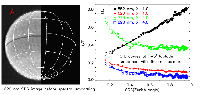
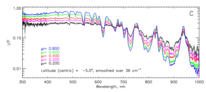
Figure 7.— A: Sample image from the unsmoothed KT2009 STIS data cube at 620 nm, with grayed pixels indicating our center-to-limb sampling at 5^∘ S, with grid lines at 30^∘ intervals. B: Sample center-to-limb scans at four wavelengths (after spectral smoothing with a 36 cm^-1 boxcar), with fits shown by dot-dash lines bounding 1$\sigma$ uncertainty limits. C: Sample interpolated STIS I/F spectra at 5^∘ S planetocentric latitude after CTL fitting and spectral smoothing.

The sensitivity of these spectra to different atmospheric levels on Uranus is indicated in Fig. 8. This indicates the penetration depth of light into an aerosol-free atmosphere of Uranus by the plot of pressures at which one-way unit vertical optical depth is reached. Penetration depths for individual contributions by Rayleigh scattering, methane absorption and hydrogen collision-induced absorption (H₂ CIA) are also shown. A key wavelength region is near 0.825 $\mu$m, where H₂ CIA opacity exceeds the opacity of methane. Poor fits in this region are an indication of incompatible vertical distributions of methane and hydrogen absorptions, and may be a result of assuming an incorrect methane mixing ratio.

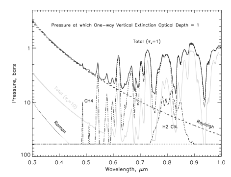
Figure 8.— Pressure at which the vertical optical depth to space reached unity, shown for individual components including Raman scattering (dotted), Rayleigh scattering (dashed), methane absorption (triple-dot-dash), and H₂ CIA (dot-dash). The pressure for all effects combined is shown by the dark solid curve for unit optical depth and by the light solid curve for $\tau=10$.

4.2. Radiation transfer calculations

We used the radiation transfer code described by Sromovsky (2005a), which include Raman scattering and polarization effects on outgoing intensity. To save computational time we employed the accurate polarization correction described by Sromovsky (2005b). After trial calculations to determine the effect of different quadrature schemes on the computed spectra, we decided to use 14 zenith angle quadrature points per hemisphere and a 14-order azimuthal expansion for our compact model and 10 quadrature points for fitting models with the KT2009 structure. To characterize methane absorption we used the corrected coefficients of KT2009. To model collision-induced absorption (CIA) of H₂-H₂ and He-H₂ interactions we interpolated tables of absorption coefficients as a function of pressure and temperature that were computed with a program provided by Alexandra Borysow (Borysow et al. 2000), and available at the Atmospheres Node of NASA’S Planetary Data System. We assumed equilibrium hydrogen for most calculations but did look into the effects of non-equilibrium distributions, which are discussed in Sec. 8.2

4.3. Cloud models

We used two distinct models of cloud structure for comparison purposes. The first is nearly identical to the model of KT2009, which we will refer to as the KT2009 model, and the second is a modified version, which we will refer to as the compact cloud layer model. A plot of the vertical distribution of these layers can be found in Sec. 5.3 (Fig. 14).

4.3.1 The KT2009 model

This model has four layers of aerosols, the uppermost being a Mie-scattering stratospheric haze layer characterized by an optical depth at 0.9 $\mu$m, a gamma size distribution (Hansen 1971), with a mean radius of $a=$0.1 $\mu$m and a normalized variance of $b=$0.3. These particles are assumed to have a real index of 1.4, and an imaginary index following the KT2009 relation

$$n_{i}(\lambda)=0.055\exp[(350-\lambda)/100],$$ (6)

for $\lambda$ in nm. This haze was distributed vertically above the 100 mb level with a constant optical depth per bar. The remaining layers in the KT2009 model are characterized by a wavelength-independent optical depth per bar and a wavelength-dependent single-scattering albedo, given by

$$\varpi_{t}(\lambda)=1-1/[2+\exp[(\lambda-290)/37]],$$ (7)

again for $\lambda$ in nm. Their adopted double Henyey-Greenstein phase function for the tropospheric layers used $g_{1}=$0.7, $g_{2}$=-0.3, and a wavelength-dependent fraction for the first term, given by

$$f_{1}(\lambda)=0.94-0.47\sin^{4}[(1000-\lambda)/445],$$ (8)

which produces a backscatter that decreases with wavelength, as shown in Fig. 9. The three tropospheric layers are uniformly mixed with gas molecules, with different optical depths per bar in three distinct layers: 0.1-1.2 bars (upper troposphere), 1.2-2 bars (middle troposphere), and P$>$2 bars (lower troposphere). These optical depths are the adjustable parameters we use to fit this model to the observations.

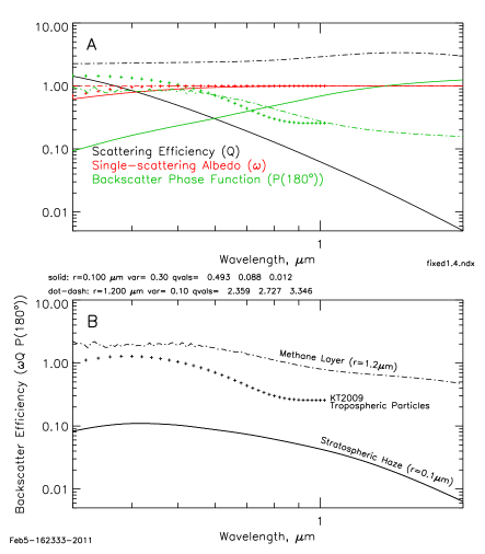
Figure 9.— Scattering properties of the stratospheric haze model (solid), the middle tropospheric Mie layer (dot-dash) and KT2009 tropospheric particles (plus signs). A: extinction efficiency (Q, black), single-scattering albedo ($\varpi$, red) and backscatter phase function ($P(\pi)$, green). B: backscatter efficiency.

4.3.2 The compact cloud layer model

This model is a modification of the KT2009 model. The main change we made is to replace their middle tropospheric layer with two compact layers: an upper tropospheric compact cloud layer and a middle tropospheric compact cloud layer. This allows the possibility of a better match to the observations if the aerosols between 1 and 2 bars do not match the KT2009 assumption of being uniformly mixed with the gas. The upper tropospheric cloud (UTC) in our model is composed of Mie particles, which we characterized by a gamma size distribution with a mean particle radius of 1.2 $\mu$m and a fixed normalized variance of 0.1, a fixed refractive index of 1.4, and an imaginary index of zero. The particle radius was fixed at the given value because it did not vary much from that value in preliminary fits. For the middle tropospheric cloud (MTC) in our model we used particles with the same scattering properties as given by KT2009 for their tropospheric particles. Both of these compact layers have the bottom pressure as a free (adjustable) parameter and a top pressure that is a fixed fraction of 0.93 of the bottom pressure. This degree of confinement is approximately the same as obtained for the cloud layer inferred from the occultation analysis. We assumed similar confinement for the deeper layer in our model, but it could easily be more vertically diffuse than we assumed, as long as the effective pressure is similar.

The last change we made was to replace their lower tropospheric layer by a compact cloud layer at 5 bars (the LTC), with adjustable optical depth and with the KT2009 tropospheric scattering properties. We found that this layer was needed to provide accurate fits near 0.56 and 0.59 $\mu$m, but its pressure is not well constrained by the observations (the effect of varying the pressure can be compensated by varying the optical depth, to produce essentially the same fit quality). Whether this deep cloud is vertically diffuse or compact also cannot be well constrained, and thus our assumption of a compact cloud for this layer is a matter of convenience and is not compelled by observations. The wavelength dependence of the backscatter phase function, extinction efficiency, and single scattering albedo of the stratospheric haze are given in Fig. 9 for both the Mie particles we used for the putative methane layer (the UTC) and for the KT2009 tropospheric particles. The latter have wavelength independent optical depth, and thus the way its backscatter efficiency varies with wavelength is entirely determined by the phase function (defined by Eq. 8). The best-fit Mie particle size results in a smaller variation in backscatter efficiency, although both decrease with wavelength.

In summary, we consider two models. The diffuse one has the KT2009 structure, which provides a fitting standard of comparison. The compact model, the main feature of which is the splitting of the middle tropospheric layer of KT2009 into two layers, allows us to see if a compact layer of methane particles can provide good fits to the observed spectra, and to see which occultation-derived profile of temperature and methane mixing ratio provides (1) the best fit to the spectra and (2) the best agreement between the fit pressure for the middle tropospheric layer and the pressure inferred from the occultation analysis. Hopefully, the best spectral fit would occur for the same profile that provided the best pressure match. As shown in the following, that is roughly what happened.

4.4. Error model

To measure fit quality we use $\chi^{2}$, which requires an estimate of the expected difference between a model and the observations due to the uncertainties in both. We roughly characterized the uncertainty in measurements by the expected uncertainty in the samples of the smooth fits, as described previously. This uncertainty is shown by the purple curve in the upper panel of Fig. 10. There is also an overall calibration uncertainty, estimated by KT2009 to be 5%. However, calibration errors for spectra are similar to nearly wavelength-independent scale factor errors, which tend to cause changes in inferred optical depths of aerosols, with very little effect on their inferred vertical distributions, and thus we did not include this as an error source. KT2009 estimated relative uncertainties of their corrected spectra to be within 1%, which were estimated by comparison of the corrected spectrally weighted STIS observations to band-pass filtered images. To this relative calibration uncertainty we added an overall modeling uncertainty of 1% for a combined relative fractional error of 1.4%, shown by the red curve in Fig. 10. Another important source of uncertainty is due to uncertainty in the methane absorption coefficients, which is not easy to characterize. We assumed that the uncertainty in $k$ had the form $\epsilon(k)=\alpha k+\epsilon_{0}$, where we adopted values of $\alpha=0.02$ and $\epsilon_{0}$ = 5$\times 10^{-4}$ km-am. The 2% scale-factor component ($\alpha$) is roughly in agreement with the verification provided by the Descent Imager/Spectral Radiometer (DISR) measurements within Titan’s atmosphere (Tomasko et al. 2008) over the 0.5-0.75 $\mu$m wavelength range, though larger errors are indicated at longer wavelengths. The offset error is even less certain. KT2009 made changes as large as 0.01 km-am from previous coefficients (Karkoschka 1998), and the new values, which we use here, are likely to be much smaller, but by exactly what factor is unclear.

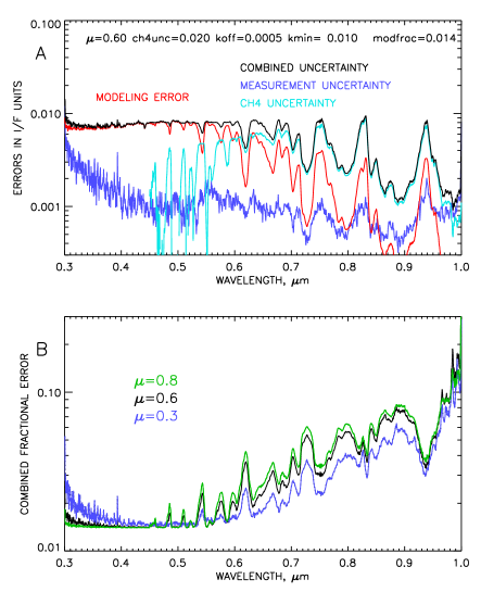
Figure 10.— A: Estimated contributions by measurement uncertainty (purple), methane coefficient uncertainty (blue), and overall modeling errors (red), to the combined relative I/F uncertainty for $\mu$=0.6 (black). B: Combined Fractional error vs. wavelength at zenith angle cosines of 0.3 (purple), 0.6 (black), and 0.8 (green).

We used a refinement of the approach of Sromovsky and Fry (2010) in approximating the effect of methane absorption uncertainty on the spectrum. We used a similar crude approximation, that the reflected intensity at any wavelength could be expressed as a maximum times an exponential in optical depth, i.e.

$$I(\lambda,\mu) = I_{0}(\mu)\exp(-ku/\mu)$$ (9)

where the optical depth is $ku$, $k$ is the absorption coefficient, and $u$ is the absorber path amount. This directly leads to a fractional error in I/F given by

$$\delta I/I=1-[I(\lambda,\mu)/I_{0}(\mu)]^{\alpha+\epsilon_{0}/k}$$ (10)

which differs from the model of Sromovsky and Fry (2010) by using the maximum $I_{0}(\mu)$ instead of unity, and by including the $\epsilon_{0}/k$ term in the exponent. That term becomes dominant for small $k$, and expresses the fact that small absorptions that cause large I/F depressions lead to large uncertainties because the offset uncertainty begins to be comparable to the total absorption coefficient. However, in this crude form the term becomes unstable when the absorption is very small and $I/I_{0}$ is near 1, but where (because of our crude model) it is not close enough to 1 to make the $\epsilon_{0}/k$ term unimportant. To counteract this instability we replace $\epsilon_{0}/k$ with $\epsilon_{0}/(k+k_{\mathsf{min}})$, where we chose $k_{\mathsf{min}}$=0.01 to avoid excessively large errors for $\lambda<$ 0.5 $\mu$m. The final form of this model is shown as the CH₄ uncertainty in Fig. 10. This was treated as normally distributed with the standard deviation as shown, which is another crude assumption. However, it is likely that the overall dominance of this error source at wavelengths exceeding about 0.6 $\mu$m is correct.

Our final combined error estimate was the square root of the sum of the squares of the three sources. Although these error sources are not accurately known or well characterized by our noise model, they can be roughly validated by comparing, for the best fit over all models and profiles, the minimum $\chi^{2}$ value with the expected value for a perfect fit. Our very best fit over this spectral range (at this latitude) yielded approximately 339 for $\chi^{2}$ instead of the value of 269 predicted by the error model. This would be the result of under-estimating the combined errors by 12%, or by a defect in the physical model we are using to fit to the observations (at other latitudes we obtained $\chi^{2}$ values as low as 269).

4.5. Fitting procedures

To avoid the need for fitting an imaginary index in the methane layer (the UTC layer) we fit only the wavelength range from 0.55 $\mu$m to 1.0 $\mu$m. To provide a reasonable computational speed while still sampling a wide range of penetration depths for each spectral band, we chose a wavenumber step of 118.86 cm^-1 for sampling the observed and calculated spectrum. This yielded 69 spectral samples, each at four different zenith angle cosines (0.3, 0.4, 0.6, and 0.8), for a total of 276 points of comparison. Our compact layer model has seven adjustable parameters (pressures and optical depths of the UTC and MTC layers, the optical depth per bar of the stratospheric haze, the optical depth per bar of the upper tropospheric haze (KT2009 referred to this as the upper tropospheric layer), and the optical depth of the LTC layer, leaving 269 degrees of freedom. We fixed the LTC base pressure to 5 bars and the UTC mean particle radius at 1.2 $\mu$m because these values were consistently obtained for a variety of fits, and reducing the number of adjustable parameters improved fit algorithm performance. Furthermore, the LTC pressure is not well constrained by the observations because its change can be compensated by changing the LTC optical depth. To fit the KT2009 model over the same range, we followed their approach by adjusting only the four $d\tau/dP$ (optical depth per bar) values. We use a modified Levenberg-Marquardt non-linear fitting algorithm (Sromovsky and Fry 2010) to adjust the fitted parameters to minimize $\chi^{2}$ and to estimate uncertainties in the fitted parameters. The uncertainty in $\chi^{2}$ is expected to be $\sim$25, and thus fit differences within this range are not of significantly different quality.

5. Application of Spectral Constraints to the Occultation Solutions

5.1. Fit results for 5^∘ S

The fit results for the compact model for profiles D1, E1, EF, F1, and G are given in Table 2 and key results are plotted as a function of methane volume mixing ratio in Fig. 11. The parameters of the aerosol model are very well constrained by the observations, with pressures constrained to a fraction of a percent and optical depths usually to within 5%. In Fig. 11 we show several results that can be used to constrain the methane mixing ratio at 5^∘ S: (A) the pressure of the upper tropospheric cloud (UTC) in comparison with the occultation cloud pressure, (B) the overall quality of the spectral fit, (C) the fit error at 0.825 $\mu$m, and (D), the He/H₂ ratio.

The results for cloud pressure (Fig. 11 A) show that the upper compact cloud (modeled as methane) is in best agreement with the occultation pressure range at a methane mixing ratio of 4.0%, but the match is still fairly close down to a mixing ratio near 3.5%. An even stronger constraint on the CH₄ mixing ratio is the fitting error in the region near 0.825 $\mu$m (Fig. 11B), where hydrogen CIA exceeds methane absorption. If there is too much methane assumed in our model, then model cloud particles will need to move upward to compensate. That will place them relatively further above the absorption of hydrogen, and where the effects of hydrogen can be seen (as at 0.825 $\mu$m) the model will appear too bright relative to the observations. Where the assumed CH₄ mixing ratio is too low (as for Model D1 at 5^∘ S) the model I/F will appear be too low at 0.825 $\mu$m. This constraint clearly favors a mixing ratio of 4.5% with an uncertainty of roughly 0.7%. The overlap of the first two uncertainty ranges is 3.8-4.5%. The third constraint is overall fit quality (Fig. 11 C). The best spectral fit (judged from the minimum $\chi^{2}$ in the middle panel) is for a methane mixing ratio near 3.6%, but the fit is nearly as good over a wide range from 3-4.9%. This is a relatively weak constraint that is easily compatible with the previous stronger constraints, which favor a mixing ratio of 4%. This makes our Model F1 profile the preferred profile, even though it slightly exceeds the Conrath et al. (1987) uncertainty limits of the He VMR, as shown in Fig. 11D. We consider E1, EF, and F1 profiles plausible candidates for further analysis. Our preferred model (F1) leads to a compact methane condensation cloud very close to pressure level expected from occultation results and it is also a model that provides an excellent fit to the STIS spectral observations, especially in the key region where hydrogen CIA is significant.

Table 2Best-fit parameters for compact cloud layer models at 5^∘ S.

OCCULTATION PROFILE:	D1	E1	EF	F1	G
KEY PROFILE PARAMETERS:
Cloud Top, bar	1.136	1.142	1.142	1.146	1.153
Cloud Bottom, bar	1.251	1.241	1.226	1.221	1.205
Deep Methane VMR	2.22%	3.24%	3.64%	4.00%	4.88%
AEROSOL PARAMETERS:
$(d\tau/dP)_{\mathsf{Strat.H}}$, bar-1	0.329	0.208	0.178	0.158	0.136
$(d\tau/dP)_{\mathsf{UTH}}$, bar-1	0.01	0.032	0.035	0.038	0.031
$P_{\mathsf{UTC}}$, bar	1.45	1.27	1.24	1.23	1.19
$P_{\mathsf{MTC}}$, bar	2.54	1.80	1.72	1.68	1.60
$P_{\mathsf{LTC}}$, bar	5.	5.	5.	5.	5.
$\tau$UTC	0.444	0.328	0.324	0.322	0.324
$\tau$MTC	1.33	1.16	1.23	1.28	1.42
$\tau$LTC	0.01	2.30	2.92	3.45	4.75
$r$Strat.H, $\mu$m	0.1	0.1	0.1	0.1	0.1
$r$UTC, $\mu$m	1.2	1.2	1.2	1.2	1.2
FIT QUALITY:
$\chi^{2}$(total)	435.6	340.5	338.5	342.3	351.9
$\chi^{2}$(0.825 $\mu$m)	47.7	11.0	5.1	2.2	0.6
Fit error at 0.825 $\mu$m, $\mu$=0.8	-4.54	-2.14	-1.34	-0.71	+0.54

Note: The uncertainty in $\chi^{2}$ is $\sim$25 and thus fits differing by less than this are not of significantly different quality. The stratospheric haze base extends upward from 100 mb, the upper tropospheric haze (UTH) extends from 900 mb to 100 mb, The upper tropospheric cloud (UTC) and middle tropospheric cloud (MTC) extend from the bottom pressures, tabulated here, to 0.93 times those pressures. The lower tropospheric cloud is bounded by the tabulated base pressure and 0.98 times that pressure. For these fits, the particle radii of the Mie layers were held fixed, as was the pressure of the lower tropospheric cloud. The fit error at 0.825 $\mu$m is the ratio of (model-measured) to estimated uncertainty.

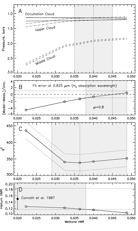
Figure 11.— Fit results for compact cloud layer models as a function of the deep volume mixing ratio of methane (points are plotted for models D1, E1, EF, F1, and G from left to right). A: pressures of the upper (presumably CH₄) and middle tropospheric cloud models compared to the cloud layer inferred from our occultation analysis (solid lines). B: Fit error at 0.825 $\mu$m where hydrogen CIA is prominent. C: Minimum $\chi^{2}$ values (solid line) for fits to spectra at 4 zenith angles and 69 wavelengths from 0.55 to 1.0 $\mu$m, with dotted lines indicating the 1$\sigma$ uncertainty range expected for $\chi^{2}$. D: He volume mixing ratio (line) compared to the Conrath et al. (1987) value (symbol with error bars). The grayed areas indicate rough regions of uncertainty/acceptability.

The best compact cloud model fit to STIS spectra at 5^∘ S using the F1 profile (shown in Fig. 12) yielded an uncorrected $\chi^{2}$ of 342, which is significantly better than the best $\chi^{2}$ values of 409, 426, and 458 obtained by our fit of the KT2009 model to E1, EF, and F1 profiles respectively. Thus, we don’t have to give up anything in fit quality to obtain the compatibility between aerosol models and occultation models. In fact, the fit quality improves, as one would expect with two more adjustable parameters available.

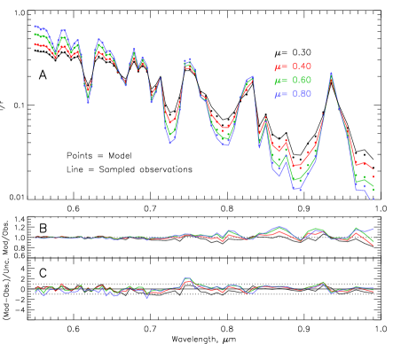
Figure 12.— A: STIS 5^∘ S spectra (solid lines) at four zenith angles, sampled at a wavenumber spacing of 118.86 cm^-1, compared to model calculations (points) for the model that best fits the spectrum when the F1 profile of temperature and methane mixing ratio is assumed. B: Ratio of Model to observed I/F values. C: Difference of model and observed values divided by the expected uncertainty at each wavelength sample. Note that the larger fractional errors that occur for $\lambda>$0.78 $\mu$m are within the expected range of uncertainties.

Our presumed methane cloud has an effective particle radius near 1.2 $\mu$m and a rather small optical depth, only about 0.32 at $\lambda=$ 0.5 $\mu$m, which about half the value reported by Rages et al. (1991) for their low latitude cloud, but close to the 0.4 value of Baines et al. (1995) for a disk average that weighted high latitudes most. The middle tropospheric cloud is considerably thicker, with an optical depth of 1.23 for the optimum methane profile. The much deeper lower tropospheric cloud is generally even thicker, except for the model D1 profile for which this cloud is not even needed.

5.2. Layer contributions

The relative roles played by our five model layers in creating the observed spectral characteristics are illustrated in Fig. 13B-F, which displays the effect of removing each layer from the model spectrum. The distinctly different contributions of the various layers is what allows the model parameters to be so well constrained by the observations. We see in B that the stratospheric haze (layer 1) serves to reduce the I/F for $\lambda<0.6$ $\mu$m and provide a slight (5-10%) boost to the I/F in the center of the deep absorption bands at longer wavelengths. As shown in C, the upper tropospheric haze layer (layer 2) makes a similar contribution but without as much shortwave absorption. The methane cloud (layer 3, panel D) contributes almost nothing at wavelengths less than 0.55 $\mu$m but provides a significant contribution to minima in the intermediate absorption bands and especially to the shoulders of the strong absorption bands. The effect of the middle tropospheric cloud (layer 4, panel E) is seen mainly in the strong contributions to the I/F peaks, and also in contributing a small absorption peaking near 0.4 $\mu$m. The lower tropospheric cloud (layer 5, panel F) contributes mainly to the longer wave window regions, and is unique in providing key contributions at 0.55 and 0.59 $\mu$m. Note that, although the model fit was only constrained by measurements from 0.55 to 1.0 $\mu$m, it provides a relatively good fit to the shorter wavelengths as well (panel A). The discrepancies between model fit and measurements between 0.3 and 0.4 $\mu$m are only about 10% and could be largely removed by slight increases in the lower tropospheric cloud absorption and slight decreases in the stratospheric haze absorption in this region. It might also be possible to introduce some of the extra absorption needed at small zenith angles into the methane layer itself, as suggested by Rages et al. (1991).

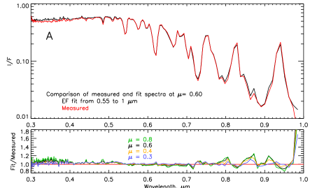
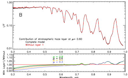
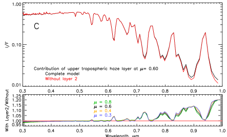
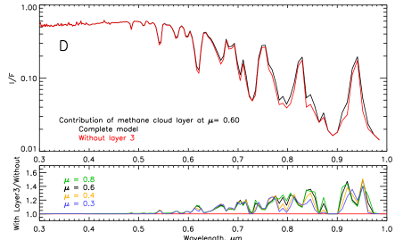
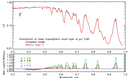
Figure 13.— A: Comparison of measured STIS spectrum (red) at 5^∘ S with a compact model fit (black), with spectra shown at a solar zenith angle cosine of 0.6 and ratios shown for all four cosine values); B-F: Comparisons of the model spectrum with spectra for same model with layers 1-5 removed respectively. Layer 3 (D) is the methane cloud layer. Although these spectral sensitivities were calculated for the EF profile, they also closely represent results for E1 and F1 profiles.

5.3. Comparison of vertical structures

The vertical structure of our compact cloud model and the diffuse vertical structure of the KT2009 model are compared directly in Fig. 14, which displays optical depth per unit pressure versus pressure (A) and cumulative optical depth versus pressure (B). There is a very large difference in the vertical distribution of cloud particles, with our compact model providing high opacity concentrations in narrow pressure ranges. But when compared on the basis of cumulative opacity we see that the KT2009 model looks like a vertically averaged version of our results. The compact layer with the strongest effect on the CCD spectrum is our layer 4 (MTC), as shown in Fig. 13. The dashed line in Fig. 14A is for optical depth per bar at 1.6 $\mu$m from Fig. 5 of Irwin et al. (2010) with pressures scaled by the factor 1.8/2.6 to account for the decrease indicated in their Fig. 8, when they used a vertical methane profile similar to the L87 Model F. Their relative vertical distribution of opacity is crudely consistent with that of the other models, when vertical smoothing is taken into account. However, the quantitative values of their opacities per unit pressure are hard to compare with our (or KT2009) results because of very different assumptions made about particle scattering properties, including the extreme assumption that particle scattering properties were independent of latitude and altitude.

While the top compact layer in our model is consistent with condensation of methane, the composition of the deeper layers is highly uncertain. Possible parent gases are H₂S and NH₃, but condensation layers at 1.7-3 bars would imply strong depletions from their expected deep mixing ratios, which is plausibly an effect of the formation of a much deeper cloud of NH₄SH particles, as discussed by de Pater et al. (1989) and Fegley et al. (1991).

Figure 14.— Optical depth per bar (A) and cumulative optical depth (B) for a vertically diffuse KT2009 model (dotted) and out compact layer model (solid) fit to 5^∘ S STIS spectra using the F1 vertical profile of temperature and methane mixing ratio. For the KT2009 model we fit the four optical depths per bar, and used the KT2009 values for pressures and particle scattering properties. For our model we fit two optical depths per bar for the upper two layers and the pressures and optical depths of the three compact layers, except for the fixed 5 bar pressure we used for the bottom layer. The dashed line in A is optical depth per bar at 1.6 $\mu$m from Fig. 5 of Irwin et al. (2010) with pressures scaled by the factor 1.8/2.6 to account for the decrease indicated in their Fig. 8, when they used a vertical methane profile similar to the L87 Model F.

6. Latitude dependence of methane on Uranus

We first show that the occultation solution that is most consistent with low latitude spectra is not consistent with high-latitude spectra and then discuss how that profile can be modified in physically reasonable ways and which modifications provide the best fits at high latitudes.

6.1. Fit results assuming latitude-independent methane

EF and F1 model temperature and methane profiles yielded high quality spectral fits not only at the occultation latitude, but also for latitudes from 30^∘ S to 20^∘ N, as indicated in Fig. 15A for the F1 fits. Over this latitude range the fit quality was generally very high, reaching $\chi^{2}$ values close to those expected from the error model, and about half were notably better than we obtained at 5^∘ S. However, between 30^∘ S and 45^∘ S fit quality began to deteriorate dramatically, with $\chi^{2}$ growing to $\sim$1100 by 60^∘ S, which is four times the expected value. At the same time, at 0.825 $\mu$m, where hydrogen CIA is an important contributor, the $\chi^{2}$ contribution (Fig. 15B) and the signed fit error (Fig. 15C) remained relatively flat over the 30^∘ S to 20^∘ N region, but grew dramatically from 30^∘ S to 60^∘ S, with the signed error reaching 7 times the expected uncertainty and the $\chi^{2}$ contribution reaching more than 40 times the expected value. Thus, there is little question that the methane mixing ratio at high latitudes is quite different from what it is at middle latitudes, a result already established by KT2009. To get a more realistic picture of the high latitudes, we need to estimate what the actual methane mixing ratio profile is at these latitudes. In the next section we discuss plausible ways to modify our baseline (F1) profile so that we can investigate this issue.

Figure 15.— Spectral fit quality measured by $\chi^{2}$ over the entire range of the fit (A) and $\chi^{2}$ for the 4 view angles at the 0.825 $\mu$m H₂ CIA wavelength (B), and fit error at 825 nm and $\mu$=0.8 (C), all as a function of planetocentric latitude, using the F1 temperature and methane profiles. Filled circles in A denote results of fitting the KT2009 structure model. The horizontal dotted lines in A and C indicate expected (central) and 1$\sigma$ uncertainty bounds.

6.2. Construction of depleted methane profiles

The occultation places no direct constraints on the temperature or methane profiles at other latitudes. However, there are some reasonable physical constraints to consider. First, the lack of significant latitudinal gradients in the temperatures inferred from Voyager 2 IRIS observations for P$>\sim$150 mb (Hanel et al. 1986) suggests that the occultation thermal profile is a good approximation at all latitudes on Uranus. A second constraint has to do with an extension of the relationship between the vertical wind shear and horizontal temperature gradients. The variation of mixing ratio with latitude, assuming the same pressure-temperature structure at all latitudes (as assumed by KT2009 as well), leads to a variation in density on constant pressure surfaces, which is similar in effect to horizontal temperature gradients. Both kinds of gradients lead to vertical wind shear (Sun et al. 1991), a consequence of geostrophic and hydrostatic balance. If such latitudinal variations occurred through great atmospheric depths, this would lead to great differences in cloud level winds and conflict with the observed wind structure of Uranus. Thus we expect that where methane is depleted, it is not depleted over great depths. And, as indicated by KT2009, the spectral observations do not require that methane depletions extend to great depths. In fact, we will later show that the spectral constraints favor relatively shallow methane depletions.

For trial purposes we created several types of modifications of the F1 profile. We first defined an upper tropospheric mixing ratio and a set of transition pressures, $P_{1}$ and $P_{2}$. for $P>P_{2}$ we kept the mixing ratio at the F1 deep value of 4%. For $P<P_{1}$ we set the mixing ratio to the upper level value, except where that value exceeded the F1 value above the methane condensation level, at which point we reverted to the F1 model profile. Between the two transition pressures we interpolated between the upper troposphere and deep values. Sample depleted profiles of this type are shown in Fig. 16A. These profiles are consistent with methane condensation at somewhat lower pressures than for the F1 profile. A depleted profile of this type might be created by descent of the low-mixing-ratio gas from slightly above the 1.2 bar level downward to higher pressures, but to limited depths.

We also considered “proportionally descended gas” profiles in which the model F1 mixing ratio profile $\alpha(P)$ was dropped down to increased pressure levels $P^{\prime}(\alpha)$ using the equation

$$P^{\prime}=P\times[1+(\alpha/\alpha_{d})^{vx}(P_{d}/P_{cb}-1)]$$ (11)

$$\mathrm{for} P_{tr}<P<P_{d},$$

where $P_{d}$ is the pressure depth at which the revised mixing ratio $\alpha^{\prime}=\alpha(P^{\prime})$ equals the uniform deep mixing ratio $\alpha_{d}$ , $P_{cb}$ is the cloud bottom pressure (which is where the unperturbed profile departs from the uniform deep value), $P_{tr}$ is the tropopause pressure (100 mb), and the exponent $vx$ controls the shape of the profile between 100 mb and $P_{d}$. A sampling of profiles of this type are shown in Fig. 16B. The profiles with $vx=1$ are similar in form to those adopted by Karkoschka and Tomasko (2011). A profile of this type is consistent with the descending gas beginning at lower pressures than for our initial set of models. In both cases we would expect methane condensation to be inhibited by the downward mixing of upper tropospheric gas of low methane mixing ratios. How these various types of profiles affected fits to the 45^∘ S and 60^∘ S spectra is discussed in the next section.

Figure 16.— Sample profiles of depleted methane used to fit high-latitude STIS spectra. The undepleted base profile labeled by its valid latitude range of 30^∘ S to 20^∘ N is from Model F1. The profiles in A provided the best fits for the indicated latitudes. None of the B profiles yielded any better fits (see text).

6.3. Constraining methane profiles at 60^∘ S and 45^∘ S

We used our 5-layer model, allowed adjustment of all 9 parameters, and tried CH₄ mixing ratios as low as 0.3% in the depleted region, and transition depths ranging from 1.5-2 bars to as deep as 9-10 bars. The bottom of the transition region is where the F1 deep mixing ratio of 4% is reached. The results were evaluated by comparing their overall fit quality (how low their $\chi^{2}$ values were) and how big their fitting errors were at the key wavelength of 0.825 $\mu$m, where H₂ CIA is an important contributor. The results are summarized in Fig. 17 for depletion depths of 1.5-2 bars (only for 45^∘ S), 2-3 bars, 4-6 bars, and 9-10 bars. At neither latitude is it possible to obtain a good fit with deep depletions that extend to 9-10 bars. Although a low hydrogen fitting error can be obtained from deep depletions, the overall fit quality is much better for shallow and very strong depletions. At both latitudes lower mixing ratios lead to better fits, as long as the depletion depth is reduced as well. The minimum hydrogen error moves to lower methane mixing ratios as the depletion depth is decreased and the depletion factor is increased. It is apparent that the best combination of overall and CIA fits requires very low methane mixing ratios, of the order of 1% or even less, and shallow depletion depths, down to only 1.5-2 bars for 45^∘ S, and perhaps 2-3 bars at 60^∘ S, which are illustrated in Fig. 16A. These perturbations of the base profile are of such a small depth that the vertical wind shear caused by the resulting horizontal density gradients would not likely produce significant perturbations of the zonal wind field, though exact calculations would be needed to verify that. The depletion of methane at high latitude helps to explain the difference between prior estimates of 4% by Rages et al. (1991) and 1.1-2.3% by Baines et al. (1995), the latter weighting high latitudes more than the former.

A limited fitting exploration using more physically appealing methane profiles of the type shown in Fig. 16B did not yield significantly better fits than those shown in Fig. 16A. We did find constraints on the parameters of such profiles, however, with $vx=1$ yielding better fits than either $vx=0.5$ or $vx=2$, and $P_{pd}=2-3$ bars preferred at 45^∘ S and $P_{pd}=4-6$ bars preferred at 60^∘ S.

Figure 17.— Overall fit quality (A) and fit quality at 0.825 $\mu$m (B) versus depleted mixing ratio for planetocentric latitudes 60^∘ S (Left) and 45^∘ S (Right). The transition pressures between upper depleted regions and the deep region at 4% are noted in the legend.

These results present a picture in which dry upper tropospheric gas descends at high latitudes after being dried out by condensation of methane in upwelling gas at low latitudes, with upwelling and descending regions connected by meridional cells as illustrated in Fig. 18. The general nature of this circulation is similar to that described by KT2009 except that they don’t provide for the existence of a methane condensation cloud, which seems to us a necessary mechanism to dry out the ascending gas. The high latitude descending gas appears to be very dry and to descend only a small distance below the original methane condensation level. However, this descent should inhibit the formation of methane clouds at these latitudes, and if any do form they would have to form at much lower pressures. When we use five layers, our layer 3, which used to be found at the methane condensation level, is now found much deeper in the atmosphere and thus must be composed of some other substance, perhaps part of a somewhat extended H₂S cloud layer.

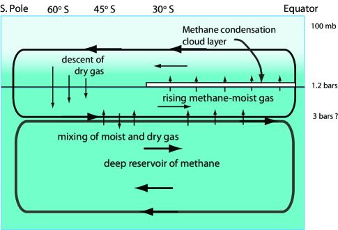
Figure 18.— Schematic of methane depletion through condensation at low latitudes as a drying process, poleward transport, then descent of dry gas, finally mixing with moist gas on the return flow. How far beyond 60^∘ S the depletion extends towards the pole, or whether northern high latitudes are depleted is unknown. Also unknown is how deep the return flow extends and whether or not there is a deep meridional flow in the opposite sense.

7. Latitude dependence of cloud structure

Our cloud pressure and optical depth parameters as a function of latitude are given in in Table 3 and key results are plotted in Fig. 19. The results for latitudes from 30^∘ S to 20^∘ N were all obtained using our F1 profile of methane and temperature. For 60^∘ S we used a methane profile depleted to 0.9% with a transition to 4% between 3 and 4 bars. At 45^∘ S, we used a depletion to 0.6% with a transition to 4% between 1.5 and 2 bars. All three of these methane profiles are shown in Fig. 16A. Looking at the low-latitude region (30^∘ S to 20^∘ N), we see that the upper compact layer (the putative methane layer, also known as the UTC or layer 3) changes pressure only slightly, remaining consistent with methane condensation at the position of that layer, while its optical depth increases slightly towards the equator before beginning a significant decline into the northern hemisphere. Somewhat more modulation is seen in the pressure of the dominant middle tropospheric cloud (MTC, layer 4) and there is a substantial declining trend in optical depth towards the north, though the rate of decline decreases near the equator. Though these declines may seem modest in the logarithmic plot, they are 7-10 times the typical 5% fitting uncertainty. The upper tropospheric haze reaches a peak opacity near the equator, as noted by KT2009.

The prominent bright band near 45^∘ S that is observed in Uranus images at wavelengths of intermediate absorption (0.1-0.4 /km-am, as shown in Fig. 23 of KT2009) is also prominent in near-IR H- and J-band images, as in Fig. 7 of Sromovsky and Fry (2007). According to Fig. 19, this band is in a region where cloud pressures have increased in both of the upper compact layers while the upper tropospheric methane mixing ratio has decreased. It is clear that the upper compact layer at 45^∘ S and 60^∘ S cannot be the putative methane ice layer, because the pressure levels are much too high to permit condensation. It is conceivable that in this region the upper tropospheric cloud is actually what we called the middle tropospheric cloud at low latitudes. And the much deeper second compact layer may be a new cloud layer formed by the upwelling produced by the lower circulation branch in Fig. 18. This would suggest that the boundary between the upper and lower branches may be in the 1.5-1.7 bar region.

The bright band contrast relative to 60^∘ S is a result of the deeper cloud being much deeper at 60^∘ S and having a much lower optical depth. The contrast relative to lower latitudes results from a combination of reduced methane opacity as well as the extra cloud opacity in the 2-bar region, which apparently more than compensates for the absence of the 1.2-bar cloud layer and the significantly reduced opacity at 1.5 bars. At 60^∘ S the middle tropospheric cloud reaches about the same pressure as Baines et al. (1995) inferred for the semi-infinite cloud in their model, which is heavily weighted towards high latitudes.

Figure 19.— Cloud model parameters as a function of latitude, from Table  3. The Upper Tropospheric cloud from 30^∘ S to 20^∘ N is consistent with a methane cloud. There appears to be no methane cloud at 45^∘ S and 60^∘ S. The largest effect on the STIS spectra is produced by the Middle Tropospheric Cloud. The filled circle in A marks the top of the optically thick cloud of Baines et al. (1995), plotted at the sub-earth latitude of the disk-integrated observations they analyzed.

Table 3Fit parameters at 10 latitudes, using Model F1 profiles for all but 45^∘ S and 60^∘ S.

Centric	$P_{\mathsf{UTC}}$	$P_{\mathsf{MTC}}$	$(d\tau/dP)$	$(d\tau/dP)$
Latitude	bars	bars	Strat.Haze	UT. Haze	$\tau$UTC	$\tau$MTC	$\tau$LTC	$\chi^{2}$
20∘ N	1.185	1.565	0.230	0.0000	0.163	0.86	2.74	372
10∘ N	1.175	1.595	0.334	0.0019	0.213	1.17	4.16	269
4∘ N	1.180	1.558	0.148	0.0363	0.269	1.15	3.83	394
0∘	1.192	1.585	0.185	0.0531	0.291	1.22	3.89	351
5∘ S	1.225	1.676	0.158	0.0375	0.322	1.28	3.45	342
10∘ S	1.224	1.649	0.280	0.0098	0.297	1.40	4.68	281
20∘ S	1.222	1.622	0.262	0.0043	0.248	1.48	5.48	282
30∘ S	1.192	1.500	0.075	0.0246	0.265	1.53	5.85	311
45∘ S	1.533	2.074	0.234	0.0181	0.393	2.24	21.4	435
60∘ S	1.589	3.131	0.206	0.0493	0.445	0.67	23.8	444

Note: Fixed parameters (except at 45^∘ S and 60^∘ S) included the lower cloud base pressure (5 bars), the particle radius of the upper tropospheric cloud (1.2 $\mu$m ). At 45^∘ S and 60^∘ S, we used $r_{UTC}=1.1$ and 1.34 $\mu$m , and $P_{LTC}=8$ and 11 bars, respectively.

8. Discussion

8.1. Occultation failure to detect the middle tropospheric cloud

Because the occultation probes to higher pressures than the pressures we infer for the dominant middle tropospheric cloud, one might wonder why the occultation did not detect this layer if it is indeed compact and created by condensation? That turns out not to be a contradiction. If the mixing ratio of the condensible is low enough, then the change in molecular weight might actually be very small, and the resulting refractivity change might be too small to be detected. For example, for H₂S to form a cloud base near 1.7 bars its volume mixing ratio would need to be $\sim$10^-7 ($\sim$0.003 times the solar mixing ratio). The maximum change in molecular weight induced by condensation of that much H₂S would then be about 3$\times 10^{-6}$, which would be completely undetectable in the occultation measurements, even if it occurred in a thin layer. But could such a cloud actually produce enough condensible material to produce the needed reflectivity of the cloud? The answer is yes. If half the H₂S gas in a 2-km thick layer were to condense into 1-$\mu$m droplets, we estimate that the resulting cloud would have about 1 optical depth. Convective processing of additional gas could increase its opacity to much higher values. NH₃ is a much less suitable candidate because its corresponding mixing ratio would be three orders of magnitude smaller as would the mass available for cloud particle formation.

8.2. Effects of para-hydrogen variations

All our calculations described so far have assumed equilibrium hydrogen, for which the para and ortho fractions are in local thermodynamic equilibrium. Since these two forms of hydrogen have different spectral features, this assumption deserves some consideration. The equilibrium para faction for our F1 profile is displayed in Fig. 20, along with several non-equilibrium curves, which we discuss in the following. In the deep atmosphere high temperatures produce a para fraction of 0.25 (referred to as normal hydrogen), but above the methane condensation level the para fraction increases dramatically. By vertically mixing deep atmospheric gas up to the cloud level and higher, a dramatic change in the para fraction can be produced, if done on a time scale short compared to the relaxation time. Baines et al. (1995) considered mixtures of equilibrium and normal hydrogen, as might be produced by vertical mixing of the high temperature para distribution with the locally equilibrated distribution. Their results were consistent with mixtures that were no less than 85% equilibrium (and thus 15% normal). KT2009 found that the difference between 100% and 85% equilibrium had a smaller effect than their uncertainties. They also stated that 50% equilibrium hydrogen would shift their results toward lower aerosol opacities and lower mixing ratios, but not change their results about latitudinal variations unless the the equilibrium fraction itself varied with latitude, which they argued against on the basis of smooth latitudinal variations in the observed hydrogen absorption regions.

Figure 20.— A: Profiles of para hydrogen assuming local thermodynamic equilibrium (solid), mixtures of equilibrium and normal hydrogen (dotted), and vertically displaced hydrogen before new equilibrium conditions are established (dot-dash). B: Example of a mixed rising-descending profile (dot-dash) compared to the equilibrium profile.

Mixtures of equilibrium and normal hydrogen cannot produce the very different para fraction profiles that can be produced by the descending or rising branches of our putative methane circulation. For convenience, we parameterize the rising or descending gas by Pfac, which is the factor by which pressure at the midpoint of the equilibrium profile is displaced. In Fig. 20A, we show para fractions that result when gas is vertically transported upward (Pfac=0.5) or downward (Pfac=1.5 and Pfac=3.0), assuming that the transport time is much less than the relaxation time to reach local equilibrium. Note that mixtures of equilibrium and normal hydrogen always decrease the para fraction, while vertical gas transport can dramatically increase or decrease the local para fraction. How changes in the para profile affect the Uranus spectrum can be seen in Fig. 21 for two profiles of the type shown in Fig. 20A: a descending gas case (Pfac=2.5) and an ascending gas case (Pfac=0.5). The effect is local, mainly between 0.77 and 0.86 $\mu$m, and is roughly the same percentage over a wide range of view angles, reaching a maximum difference of about 15%. For the case shown in Fig. 20B, where there is descending gas above 1.5 bars, and ascending gas below (deeper than) 1.5 bars, which is more consistent with high-latitude motions shown in Fig. 18, the spectral difference from the equilibrium case is only a few percent, and not detectable within current uncertainties. The fact that we did not find evidence in the spectra for significantly altered para profiles is consistent with either such a combined upwelling/down-welling profile or no significant departure from equilibrium hydrogen. However, this issue may be worth further investigation, especially if methane absorption coefficients become better known. Part of the problem making use of this constraint is that we are working with a part of the spectrum where methane absorption is weak and thus currently is significantly uncertain.

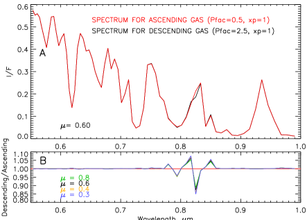
Figure 21.— A: Model spectra computed for ascending (red) and descending (black) gas profiles at view angle cosine =0.6. B: Ratio of the two spectra at four different view angle cosines.

8.3. Plausibility of a reduced He VMR on Uranus

The Voyager Infrared Radiometer Interferometer and Spectrometer (IRIS) and Radio Science Subsystem (RSS) together yielded a determination of Jupiter’s He/H₂ ratio equal to 0.114$\pm$0.025, which is a weighted mean of results by Gautier et al. (1981) and Conrath and Gierasch (1984). However, the in situ measurements of the Galileo Probe contradicted this value, instead obtaining 0.157$\pm$0.004 (von Zahn et al. 1998) and 0.156$\pm$0.006 (Niemann et al. 1998). Conrath and Gautier (2000) reviewed possible explanations for this discrepancy and ruled out IRIS calibration errors, but were unable to identify any plausible error in the occultation measurements or analysis, although a detailed error analysis of the occultation measurements was not conducted. This discrepancy also cast suspicions on the very low He/H₂ ratio obtained by IRIS-RSS analysis for Saturn, and led to an upward revision of the Saturn ratio from 0.034$\pm$0.024 to 0.11-0.16, based on a rather uncertain IRIS-only analysis (Conrath and Gautier 2000). This also raises questions about the occultation results for Uranus, suggesting perhaps that the IRIS-RSS determined ratio is actually too low for Uranus, rather than our suggestion that the ratio is too high. But an even higher ratio, with the same refractivity profile would lead to very serious amplification of inconsistencies with near-IR and CCD spectra of Uranus that have already been noted. Furthermore, because the specific error that caused prior discrepancies is not known, it is not possible to predict with any confidence how it might affect the Uranus analysis, or even what direction it might take. The change in refractivity per molecule that results from changing the He VMR from 0.15 to 0.11, as computed from Eq. 2 is from 4.496$\times 10^{-18}$ /cm³ to 4.647$\times 10^{-18}$ /cm³, which is a change of 3.3%. We do not know if an error of this magnitude is even remotely conceivable for the occultation measurements.

Figure 22.— Comparison of methane profiles from our EF and F1 models with those used by KT2009, L87, and Irwin et al. (2011), the latter following the L87 profile above the point of intersection of their assumed deep 1.6% VMR with that profile.

8.4. The reasons for higher cloud pressures obtained from Near-IR observations

The optical depth of the methane cloud is relatively small and the influence of the middle tropospheric cloud is much more significant because of its greater opacity. That and the limited vertical resolution inherent in all the spectral observations, will lead inversion methods such as the NEMESIS routine used in by Irwin and colleagues (Irwin et al. 2010, 2011) to find peak opacity contributions at pressures deeper than that of the methane cloud. In addition, these and most prior modelers of near-IR spectra assumed profiles of methane with much smaller column amounts of methane, often by a factor of two or more (Fig. 22), which leads to much higher pressures for the level of significant aerosol scattering. The dependence of derived pressure on assumed methane was clearly demonstrated by Sromovsky and Fry (2007) and by Irwin et al. (2010). As noted previously, when Irwin et al. switched from Model D to the Model F profile, the pressure of their peak opacity concentration moved from 2.5 to 1.7 bars. Since our Model F1 has more column abundance of methane down to the 1.2 bar level than even the L87 Model F, we expect similar pressures would be obtained using our recommended profile.

9. Summary and Conclusions

After reanalysis of the L87 radio occultation profiles of refractivity vs altitude, and fitting compact cloud layer models to STIS spectra as corrected and calibrated by KT2009, we reached the following main conclusions:

1. By decreasing the stratospheric He mixing ratio from its nominal value of 0.15 by 1-1.3 times its uncertainty it is possible to achieve methane saturation within the layers suspected to have condensation and to achieve increased methane humidities above the condensation level, even exceeding the high values adopted by KT2009 at low latitudes, which are inconsistent with the original L87 profiles. The maximum deep mixing ratio that we could obtain within reasonable physical constraints was 4.88% (for our model G).

2. A five-layer cloud model in which the bottom two diffuse layers of the KT2009 model are split into three compact layers, when constrained by STIS spectra at 5^∘ S, yield best-fit pressures for the top compact layer in excellent agreement with the location of the occultation cloud layer for profile models with deep CH₄ mixing ratios between 3.2 and 4.5%, with the best compromise fit being obtained at 4% (for our Model F1), although this fit is not significantly better than for the other models in this range.

3. As judged by fitting errors at 0.825 $\mu$m, where H₂ CIA exceeds methane absorption, the best compatibility between methane and H₂ CIA is obtained for a methane mixing ratio of 4.5% with an uncertainty range of about 0.7%.

4. When we consider constraints of upper cloud pressure, fit error at 0.825 $\mu$m , overall fit quality, and the uncertainty limits of the Conrath et al. (1987) helium abundance, our best compromise estimate for the deep methane mixing ratio at 5^∘ S is 4.0$\pm$0.5%, and the corresponding preferred vertical temperature and methane profiles are embodied in our F1 Model.

5. Our five-layer cloud model, using the EF and/or F1 profiles, can also provide excellent fits between latitudes of 30^∘ S and 20^∘ N, with relatively latitude-independent cloud pressure boundaries, but generally decreasing optical depths from south to north. The main exception is the upper tropospheric haze, which shows a strong peak near the equator, as noted by KT2009. The lower tropospheric cloud is found to have the greatest opacity, but the 1-2 optical depth (at 0.5 $\mu$m) middle tropospheric cloud (in 1.5-1.7 bar range) has the most significant effect on the observed CCD spectrum. The pressure of the 0.15-0.3 optical depth methane cloud layer did not vary much with latitude, staying within 2% of its 1.2 bar mean.

6. Trying to fit our model at high southern latitudes made it clear that the methane mixing ratio profile could not remain the same as we used in the low latitude observations. Not only did overall fit quality deteriorate, but the fit quality at 0.825 $\mu$m wavelength of H₂ CIA got suddenly very bad, and the direction and size of the error at that wavelength indicated a significant lowering of the methane mixing ratio, as first pointed out by KT2009.

7. We created depleted methane profiles in which depletions reached a limited depth at which point the mixing ratio transitioned to the same deep value of 4% used at low latitudes. We did not expect a depletion at great depths because the horizontal density gradients that would be generated would induce problematic vertical wind shears. Overall and 0.825 $\mu$m fit quality was found to be minimized with mixing ratios less than 1% and depletion depths of 3-4 bars at 60^∘ S and only 1.5-2 bars at 45 ^∘ S.

8. Creating the observed methane depletion is plausibly the result of upwelling at low latitudes, where the Uranus atmosphere is dried out by condensation of cloud particles, and subsequent poleward transport to and descent of the dried-out atmosphere at high latitudes down to levels of a few bars, with greater descent nearer to the pole. This would inhibit methane condensation at high latitudes and perhaps help to explain the failure to detect any discrete cloud features from 45^∘ S to the south pole.

9. The failure of modelers of near-IR spectra to detect a methane cloud at the proper location (where the occultation found a sudden change is refractivity) is due to two effects: one is that most modelers used mixing ratio profiles providing too little methane absorption and the other is that the methane cloud layer has a significantly lower opacity than the main cloud layer that peaks in the 1.4-1.7 bar region, making it hard to resolve its separate contribution.

10. The failure of the occultation measurements to detect the deeper and more significant middle tropospheric cloud layer that so prominently affects both near-IR and CCD spectra is not at all surprising if it is created by condensibles at very low mixing ratios. In that case the condensation would not produce a detectable change in refractivity.

11. Although it is not possible for the STIS spectra alone to clearly distinguish between vertically extended models, such as that of KT2009, and compact layer models of the type we presented here, there is a strong distinction in physical processes involved. Our model is consistent with cloud formation by condensation, while the KT2009 model presents a picture in which a vertically extended haze of stratospheric origin provides all the particulate opacity, much like the vertically extended haze on Titan. We prefer the condensation model because it provides consistency with the occultation observations and provides a mechanism for depleting methane from the upper troposphere at high latitudes.

Many of these results are dependent on models of methane absorption in spectral regions where absorption is relatively weak and somewhat uncertain. Some of the absorption coefficients were adjusted by KT2009 to obtain better overall fits to the observations, which might tend to favor the particular models they were using in their analysis. As we obtain more accurate information about methane absorption that is independent of the spectral observations we are trying to interpret, these conclusions may need to be modified.

The view of Uranus’ north polar regions at the beginning of 2011 is now adequate to address an important issue with new observations. The issue is whether the depletion of methane observed at southern high latitudes is also present at northern high latitudes, and if not currently depleted, whether it will become depleted as Uranus seasons proceed. There is some evidence suggesting high northern latitudes might not be depleted: discrete cloud features have been observed in 2007 Keck images between 45^∘ N and 74^∘ N (Sromovsky et al. 2009), while no discrete cloud features have been seen at corresponding southern latitudes. The lack of southern discrete features is correlated with the inferred descent of dry gas at those latitudes, suggesting that the descending gas and resulting methane depletion may not be present at high northern latitudes. The question of whether methane is currently depleted at high northern latitudes on Uranus can be answered unequivocally by new STIS spectral measurements.

References

- Baines et al. (1995) Baines, K. H., Mickelson, M. E., Larson, L. E., Ferguson, D. W., 1995. The abundances of methane and ortho/para hydrogen on Uranus and Neptune: Implications of New Laboratory 4-0 H2 quadrupole line parameters. Icarus 114, 328–340.
- Borysow et al. (2000) Borysow, A., Borysow, J., Fu, Y., 2000. Semi-empirical model of collision-induced absorption spectra of H2-H2 complexes in the second overtone band of hydrogen at temperatures from 50 to 500 K. Icarus 145, 601–608.
- Conrath et al. (1987) Conrath, B., Hanel, R., Gautier, D., Marten, A., Lindal, G., 1987. The helium abundance of Uranus from Voyager measurements. J. Geophys. Res. 92 (11), 15003–15010.
- Conrath and Gautier (2000) Conrath, B. J., Gautier, D., 2000. Saturn Helium Abundance: A Reanalysis of Voyager Measurements. Icarus 144, 124–134.
- Conrath and Gierasch (1984) Conrath, B. J., Gierasch, P. J., 1984. Global variation of the para hydrogen fraction in Jupiter’s atmosphere and implications for dynamics on the outer planets. Icarus 57, 184–204.
- Conrath et al. (1990) Conrath, B. J., Gierasch, P. J., Leroy, S. S., 1990. Temperature and circulation in the stratosphere of the outer planets. Icarus 83, 255–281.
- Costantino and Daniels (1975) Costantino, M. S., Daniels, W. B., 1975. Dielectric constant of compressed solid methane at low temperature. J. Chem. Phys. 62, 764–770.
- de Pater et al. (1989) de Pater, I., Romani, P. N., Atreya, S. K., 1989. Uranus deep atmosphere revealed. Icarus 82, 288–313.
- Fegley et al. (1991) Fegley, B. J., Gautier, D., Owen, T., Prinn, R. G., 1991. Spectroscopy and chemistry of the atmosphere of Uranus. In: Bergstralh, J. T.. and Miner, E. D. and Matthews, M. S. (Ed.), Uranus. Univ. of Arizona Press, pp. 147–203.
- Fink and Larson (1979) Fink, U., Larson, H. P., 1979. The infrared spectra of Uranus, Neptune, and Titan from 0.8 to 2.5 microns. Astrophys. J. 233, 1021–1040.
- Gautier et al. (1981) Gautier, D., Conrath, B., Flasar, M., Hanel, R., Kunde, V., Chedin, A., Scott, N., 1981. The helium abundance of Jupiter from Voyager. J. Geophys. Res. 86, 8713–8720.
- Hanel et al. (1986) Hanel, R., Conrath, B., Flasar, F. M., Kunde, V., Maquire, W., Pearl, J., Pirraglia, J., Samuelson, R., Horn, L., Schulte, P., 1986. Infrared observations of the Uranian system. Science 233, 70–74.
- Hansen (1971) Hansen, J. E., 1971. Circular polarization of sunlight reflected by clouds. Journal of Atmospheric Sciences 28, 1515–1516.
- Irwin et al. (2006) Irwin, P. G. J., Sromovsky, L. A., Strong, E. K., Sihra, K., Bowles, N., Calcutt, S. B., Remedios, J. J., 2006. Improved near-infrared methane band models and k-distribution parameters from 2000 to 9500 cm-1 and implications for interpretation of outer planet spectra. Icarus 181, 309–319.
- Irwin et al. (2010) Irwin, P. G. J., Teanby, N. A., Davis, G. R., 2010. Revised vertical cloud structure of Uranus from UKIRT/UIST observations and changes seen during Uranus’ Northern Spring Equinox from 2006 to 2008: Application of new methane absorption data and comparison with Neptune. Icarus 208, 913–926.
- Irwin et al. (2011) Irwin, P. G. J., Teanby, N. A., Davis, G. R., Fletcher, L. N., Orton, G. S., Tice, D., Kyffin, A., 2011. Uranus’ cloud structure and seasonal variability from Gemini-North and UKIRT observations. Icarus 212, 339–350.
- Karkoschka (1998) Karkoschka, E., 1998. Methane, Ammonia, and Temperature Measurements of the Jovian Planets and Titan from CCD-Spectrophotometry. Icarus 133, 134–146.
- Karkoschka (2001) Karkoschka, E., 2001. Uranus’ Apparent Seasonal Variability in 25 HST Filters. Icarus 151, 84–92.
- Karkoschka and Tomasko (2009) Karkoschka, E., Tomasko, M., 2009. The haze and methane distributions on Uranus from HST-STIS spectroscopy. Icarus 202, 287–309.
- Karkoschka and Tomasko (2010) Karkoschka, E., Tomasko, M. G., 2010. Methane absorption coefficients for the jovian planets from laboratory, Huygens, and HST data. Icarus 205, 674–694.
- Karkoschka and Tomasko (2011) Karkoschka, E., Tomasko, M. G., 2011. The haze and methane distributions on Neptune from HST-STIS spectroscopy. Icarus 211, 780–797.
- Lindal et al. (1987) Lindal, G. F., Lyons, J. R., Sweetnam, D. N., Eshleman, V. R., Hinson, D. P., 1987. The atmosphere of Uranus - Results of radio occultation measurements with Voyager 2. J. Geophys. Res. 92 (11), 14987–15001.
- Niemann et al. (1998) Niemann, H. B., Atreya, S. K., Carignan, G. R., Donahue, T. M., Haberman, J. A., Harpold, D. N., Hartle, R. E., Hunten, D. M., Kasprzak, W. T., Mahaffy, P. R., Owen, T. C., Way, S. H., 1998. The composition of the Jovian atmosphere as determined by the Galileo probe mass spectrometer. J. Geophys. Res. 103, 22831–22846.
- Orton et al. (1987) Orton, G. S., Baines, K. H., Bergstralh, J. T., Brown, R. H., Caldwell, J., Tokunaga, A. T., 1987. Infrared radiometry of Uranus and Neptune at 21 and 32 microns. Icarus 69, 230–238.
- Orton et al. (1986) Orton, G. S., Griffin, M. J., Ade, P. A. R., Nolt, I. G., Radostitz, J. V., 1986. Submillimeter and millimeter observations of Uranus and Neptune. Icarus 67, 289–304.
- Rages et al. (1991) Rages, K., Pollack, J. B., Tomasko, M. G., Doose, L. R., 1991. Properties of scatterers in the troposphere and lower stratosphere of Uranus based on Voyager imaging data. Icarus 89, 359–376.
- Sromovsky (2005a) Sromovsky, L. A., 2005a. Accurate and approximate calculations of Raman scattering in the atmosphere of Neptune. Icarus 173, 254–283.
- Sromovsky (2005b) Sromovsky, L. A., 2005b. Effects of Rayleigh-scattering polarization on reflected intensity: a fast and accurate approximation method for atmospheres with aerosols. Icarus 173, 284–294.
- Sromovsky and Fry (2007) Sromovsky, L. A., Fry, P. M., 2007. Spatially resolved cloud structure on Uranus: Implications of near-IR adaptive optics imaging. Icarus 192, 527–557.
- Sromovsky and Fry (2010) Sromovsky, L. A., Fry, P. M., 2010. The source of 3-m absorption in Jupiter’s clouds: Reanalysis of ISO observations using new NH3 absorption models. Icarus 210, 211–229.
- Sromovsky et al. (2009) Sromovsky, L. A., Fry, P. M., Hammel, H. B., Ahue, W. M., de Pater, I., Rages, K. A., Showalter, M. R., van Dam, M. A., 2009. Uranus at equinox: Cloud morphology and dynamics. Icarus 203, 265–286.
- Sromovsky et al. (2006) Sromovsky, L. A., Irwin, P. G. J., Fry, P. M., 2006. Near-IR methane absorption in outer planet atmospheres: Improved models of temperature dependence and implications for Uranus cloud structure. Icarus 182, 577–593.
- Sun et al. (1991) Sun, Z., Schubert, G., Stoker, C. R., 1991. Thermal and humidity winds in outer planet atmospheres. Icarus 91, 154–160.
- Tomasko et al. (2008) Tomasko, M. G., Bézard, B., Doose, L., Engel, S., Karkoschka, E., 2008. Measurements of methane absorption by the descent imager/spectral radiometer (DISR) during its descent through Titan’s atmosphere. Planetary and Space Science 56, 624–647.
- von Zahn et al. (1998) von Zahn, U., Hunten, D. M., Lehmacher, G., 1998. Helium in Jupiter’s atmosphere: Results from the Galileo probe helium interferometer experiment. J. Geophys. Res. 103, 22815–22830.