Abstract

Fractal Interpolation Functions (FIFs) developed through Iterated Function Systems (IFSs) offer more versatility than the classical interpolants. However, the application of FIFs in the domain of shape preserving interpolation is not fully addressed so far. Among various interpolation techniques that are available in the classical numerical analysis, the rational interpolation schemes are well suited for the shape preservation and shape modification problems. Consequently, we introduce a new class of rational cubic spline FIFs that involve tension parameters as a common platform for the shape preserving interpolation and the fractal interpolation to work together. Suitable conditions on the parameters are developed so that the rational fractal interpolant retain the monotonicity and convexity properties inherent in the given data. With some suitable hypotheses on the original data generating function, the convergence analysis of the rational cubic spline FIF is carried out. Due to the presence of scaling factors in the rational cubic spline fractal interpolant, our approach generalizes the classical results on the shape preserving rational interpolation by Delbourgo and Gregory [SIAM J. Sci. Stat. Comput., 6 (1985), pp. 967-976]. Furthermore, for preserving shape of a data set wherein the variables representing the derivatives have varying irregularity, the present schemes outperform their classical counterparts. Several examples are supplied to support the practical value of the method.
This paper was submitted to SIAM Journal of Numerical Analysis on April 14, 2013 after initial submission to Constructive Approximation on July 18, 2012.

KEYWORDS : Iterated Function System, Fractal Interpolation Function, Rational Cubic Spline FIF, Convergence, Shape Preservation, Monotonicity, Convexity.

AMS Subject Classifications: 28A80, 26C15, 26A48, 26A51, 65D05, 65D17.

1 Introduction

In the classical Numerical Analysis, there are several interpolation methods that can be applied to a specific data set, according to the assumptions that underlie the model we investigate. However, if the given data set is more complex and irregular (for instance, data sampled from real-world signals such as financial series, seismic data, and bioelectric recordings), then the traditional interpolants may not provide satisfactory results. To address this issue, Barnsley [1] introduced a class of functions called FIFs using the notion of IFS. FIFs aim mainly at data which present details at different scales or some degree of self-similarity. These characteristics imply an irregular structure to the interpolant. The main differences of FIFs from the traditional interpolants reside in: a) the definition in terms of functional equation which implies a self similarity in small scales; b) the iterative construction instead of using an analytical formula and c) the usage of some parameters, which are usually called scaling factors that are strongly related to the fractal dimension of the interpolant. Later, Barnsley and Harrington[4] observed that if the problem is of differential type, then the parameters of the IFS may be chosen suitably so that the corresponding FIF is smooth. This observation initiated a striking relationship between the classical splines and the fractal functions. Smooth FIFs (fractal splines) constitute an advance in the techniques of approximation, since the classical methods of real-data interpolation can be generalized by means of smooth fractal techniques (see, for instance, [7, 34, 35, 10]). Further, if the experimental data are approximated by a $\mathcal{C}^{r}$-FIF $S$, then the fractal dimension of $S^{(r)}$ provides a quantitative parameter for the analysis of the data, allowing to compare and discriminate experimental processes. Though FIFs are primarily applied for a self-affine/self-similar data set, their extensions namely hidden variable FIFs [3] and coalescence hidden variable FIFs [8] can be used to simulate curves that are non-self-affine or partly self-affine and partly non-self-affine in nature. Due to these versatility and flexibility, the theory of FIFs has evolved beyond its mathematical framework and has become a powerful and useful tool in the applied sciences as well as engineering.

The central focus of interpolation (traditional or fractal) is to construct a continuous function that fits the given points obtained by sampling or experimentation. However, to obtain a valid physical interpretation of the underlying process, it is important to develop interpolation schemes that inherit certain properties from the prescribed data set. Examples of few such prevalent features are positivity, monotonicity, and convexity. Constraining the range of an interpolation function so as to yield a credible visualization of the data by adhering to these intrinsic characteristics is generally referred to as shape preserving interpolation. There are multitudes of classical interpolation methods that honour shape properties inherent in the data. In what follows, we shall provide some pioneering works in this field.

Research on shape preserving interpolation has been originated with some existence-type results by Wolibner[42] and Kammerer[29]. These results do not provide any additional information on the shape preserving polynomial. A constructive approach to the shape preserving interpolation using hyperbolic tension splines was popularized by Schweikert [38]. Main issues connected with the hyperbolic tension splines are: (i) development of an automatic algorithm for the choice of free parameters is complicated; (ii) it is computationally complex to work with, especially for very large/small values of tension parameters involved in it. Polynomial splines gain shape properties either (i) by addition of extra knots (see [40, 21, 39, 33]), which may not be effective in terms of computational economy, or (ii) by perturbing derivative parameters (see, for instance, [23, 22]), which make the method unsuitable for Hermite data, where the given derivative values are also to be interpolated. In shape preservation and shape control, rational splines provide an acceptable alternative to the polynomial/hyperbolic splines. Wide applicability of the rational interpolants may be attributed to their ability to receive free parameters (which may be used for shape control) in their structure, ability to accommodate a wider range of shapes than the polynomial family, excellent asymptotic properties, capability to model complicated structures, better interpolation properties, and excellent extrapolating powers. Gregory and Delbourgo popularized the shape preserving rational interpolation methods through a series of papers [25, 18, 19, 16, 24]. These works stimulated a large amount of research in the direction of shape preserving rational spline interpolation. For brevity, the reader is referred to [13, 27, 37, 26].

These non-recursive shape preserving interpolation techniques, in general, produce smooth interpolants whose derivatives are also smooth except possibly at some finite number of points. However, in practice, there are many situations where the variable in the data possesses certain shape properties, and at the same time, variables representing the derivatives may be irregular. For instance, a sphere falling in a wormlike micellar solution does not approach a steady terminal velocity, instead, it undergoes continual oscillations as it falls [28]. Hence, to simulate the displacement and velocity profiles of such motions, monotonicity/positive interpolants with varying irregularity (fractality) in the derivatives may be advantageous. Similarly, in nonlinear control systems [41] (say, for instance, the motion of a pendulum on a cart) monotonicity/convexity preserving interpolants with varying irregularity in the second derivative may be desirable for the study of acceleration. Therefore, it is useful to develop smooth FIFs (which are known to have fractality in their derivatives) that retain the intrinsic shape properties of the data set. From the knowledge gained from the classical shape preserving polynomial interpolation techniques, it is felt that preserving fundamental shape properties via polynomial FIFs would be difficult or impossible. Thus, for an initial exposition of FIFs to the field of shape preserving interpolation, rational FIFs seem to be an appropriate medium.

With these motivations, the capability of FIFs to generalize smooth classical interpolants, and the effectiveness of rational function models in shape preservation are intertwined to provide a new solution to the shape preserving interpolation problem from a fractal perspective. We construct a $\mathcal{C}^{1}$-rational cubic spline FIF with one family of shape parameters in section 3.1. To demonstrate the effectiveness of the rational cubic spline fractal interpolation scheme, the convergence results are discussed in section 3.2. The rationale behind selecting a rational FIF with shape parameters instead of widely studied polynomial FIFs is the following. If the scaling factors tend to zero and the shape parameters tend to infinity, then the rational FIF converges to the piecewise linear interpolant for the data. This tension effect ensures that the FIF can be used for shape preserving interpolation. Section 4 provides an automatic selection of the parameters that culminate in interactive algorithms to preserve monotonicity/convexity of the data. These algorithms take full advantage of the flexibility that the fractal splines permit. By suitable choice of the shape parameters that verify the monotonicity condition, our cubic spline FIF reduces to a lower degree rational spline FIF that generalizes the classical rational spline interpolant studied in [25]. With special choices of the shape parameters satisfying convexity condition, our cubic/quadratic rational FIF reduces to lower order form, which provides the fractal generalization of the classical rational interpolant discussed in [16]. Again, by proper choices of the scaling factors and the shape parameters, our rational cubic FIF degenerates to the classical rational cubic interpolating function introduced in [19]. Therefore, the present paper offers a novel idea of setting a common platform for the fractal interpolation and the shape preserving interpolation to operate together, and in the process collectively generalizes three different classical rational interpolation schemes available in the literature. In section 5, some remarks and possible extensions are made. The effectiveness of our shape preserving fractal interpolation schemes is illustrated with suitably chosen numerical examples and graphs in section 6.

2 Basics of Polynomial Spline FIF

To equip ourselves with the requisite general material for the construction of the desired rational spline FIF, we shall reintroduce the polynomial spline FIF. A complete and rigorous treatment can be found in [1, 2, 4].

2.1 Fractal Interpolation Functions

Let $\{(x_{i},y_{i})\in I\times\mathbb{R}:i=1,2,\dots,N\}$ be a real data set, where $x_{1}<x_{2}<\dots<x_{N}$ is a partition of $I=[x_{1},x_{N}]$. Set, $K=I\times D$, where $D$ is a large enough compactum in $\mathbb{R}.$ Let $J=\{1,2,\dots,N-1\}$, and $L_{i}:I\longrightarrow I_{i}=[x_{i},x_{i+1}]$ be affine maps satisfying:

$$L_{i}(x_{1})=x_{i},\quad L_{i}(x_{N})=x_{i+1},\;i\in J,$$ (2.1)

and $F_{i}:K\longrightarrow D$ be continuous functions such that:

$$\left.\begin{split}F_{i}(x_{1},y_{1})=y_{i},\;F_{i}(x_{N},y_{N})=y_{i+1}\\ |F_{i}(x,y)-F_{i}(x,y^{*})|\leq|\alpha_{i}||y-y^{*}|\end{split}\right\},\;i\in J,$$ (2.2)

where $(x,y),(x,y^{*})\in K$, $0\leq\ |\alpha_{i}|\leq\kappa<1$ for all $i\in J$, and $\kappa$ is a fixed real constant. Define $w_{i}(x,y)=\big{(}L_{i}(x),F_{i}(x,y)\big{)}$ for $i\in J.$ It is known [1] that there exists a metric on $\mathbb{R}^{2}$, equivalent to the Euclidean metric, with respect to which $w_{i}$, $i\in J$, are contractions. The collection $\{K;w_{i},i\in J\}$ is termed as an Iterated Function System (IFS). On $\mathcal{H}(K)$, the set of all nonempty compact subsets of $K$, endowed with the Hausdorff metric, define a set valued map $W(A)=\underset{i\in J}{\bigcup}w_{i}(A)$. Then, $W$ is a contraction map on the complete metric space $\mathcal{H}(K)$. Thanks to Banach Fixed Point Theorem, there exists a unique set $G\in\mathcal{H}(K)$ such that $W(G)=G$. The set $G$ is termed as the attractor or deterministic fractal corresponding to the IFS $\{K;w_{i},i\in J\}$. The definition of a FIF originates from the following proposition:

Proposition 2.1.

(Barnsley [1]) The IFS $\{K;w_{i},i\in J\}$ has a unique attractor $G$ such that $G$ is the graph of a continuous function $f:I\rightarrow\mathbb{R}$ which interpolates the data $\{(x_{i},y_{i}):i=1,2,\dots,N\}$, i.e., $G=\{(x,f(x)):x\in I\}$ and $f(x_{i})=y_{i}~{}\text{for}~{}i=1,2,\dots,N$.

The function $f$ in Proposition 2.1 is called a fractal interpolation function corresponding to the IFS $\{K;w_{i},i\in J\}$. The adjective fractal is used to emphasize that $G=\text{graph}(f)$ may have noninteger Hausdorff-Besicovitch dimension. But $f$ may be many times differentiable (see section 2.2). Since $G$ is a union of transformed copies of itself, i.e., $G=\underset{i\in J}{\bigcup}w_{i}(G)$, an alternative name for a fractal function could be a self-referential function. The characterization of a graph of a FIF by an IFS leads to a recursive construction of $f$ using the following functional equation [1]:

$$f(x)=F_{i}\big{(}L_{i}^{-1}(x),f\circ L_{i}^{-1}(x)\big{)},\ \ x\in I_{i},\ \ i\in J.$$ (2.3)

The following special class of IFS has received wide attention in the literature:

$$\left.\begin{split}L_{i}(x)&=a_{i}x+b_{i}\\ F_{i}(x,y)&=\alpha_{i}y+R_{i}(x)\end{split}\right\},i\in J,$$ (2.4)

where $\alpha_{i}$, $i\in J,$ are parameters satisfying $|\alpha_{i}|\leq\kappa<1$ and $R_{i}:I\to\mathbb{R},\;i\in J$, are suitable polynomials satisfying (2.2). The multiplier $\alpha_{i}$ is called a scaling factor of the transformation $w_{i}$ and $\alpha=(\alpha_{1},\alpha_{2},\dots,\alpha_{N-1})$ is the scale vector of the IFS. As mentioned earlier in the introductory section, a FIF is defined in a constructive way through iterations instead of descriptive one, usually a formula, provided by the classical methods. Consequently, evaluation of a FIF at a given point needs, in general, an iteration process. An explicit representation (in terms of an infinite series) of a FIF $f$ corresponding to a general IFS (2.4) defined on $I=[0,1]$ is given in [12]. For a representation of $f$ as the uniform limit of a sequence of operators, the reader is referred to [9].

2.2 Polynomial Spline FIFs

For a prescribed data set, a polynomial FIF with $\mathcal{C}^{r}$-continuity is obtained as the fixed point of IFS (2.4), where the scaling factors $\alpha_{i}$ and the polynomials $R_{i}$ involved in (2.4) are chosen according to the following proposition.

Proposition 2.2.

(Barnsley et al. [4]) Let $x_{1}<x_{2}<\dots<x_{N}$ and $L_{i}(x)=a_{i}x+b_{i}$, $i\in J$, be the affine functions satisfying (2.1). Let $F_{i}(x,y)=\alpha_{i}y+R_{i}(x),i\in J$, satisfy (2.2). Suppose that for some integer $p\geq 0$, $|\alpha_{i}|<a_{i}^{p}$ and $R_{i}\in\mathcal{C}^{p}(I)$, $i\in J$. Let

$$F_{i,k}(x,y)=\frac{\alpha_{i}y+R_{i}^{(k)}(x)}{a_{i}^{k}},\;\;y_{1,k}=\frac{R_{1}^{(k)}(x_{1})}{a_{1}^{k}-\alpha_{1}},\>y_{N,k}=\frac{R_{N-1}^{(k)}(x_{N})}{a_{N-1}^{k}-\alpha_{N-1}};~{}~{}~{}k=1,2,\dots,p.$$

If $F_{i-1,k}(x_{N},y_{N,k})=F_{i,k}(x_{1},y_{1,k})$ for $\ i=2,3,\dots,N-1$ and $\ k=1,2,\dots,p$, then the IFS $\big{\{}\mathbb{R}^{2};\big{(}L_{i}(x),F_{i}(x,y)\big{)},i\in J\big{\}}$ determines a FIF ${f}\in\mathcal{C}^{p}[x_{1},x_{N}]$, and $f^{(k)}$ is the FIF determined by $\big{\{}\mathbb{R}^{2};\big{(}L_{i}(x),F_{i,k}(x,y)\big{)},i\in J\big{\}}$ for $k=1,2,\dots,p$.

3 Rational Cubic Spline FIFs Involving One Family of Shape Parameters

In section 3.1, we construct $\mathcal{C}^{1}$-rational spline FIFs where the inhomogeneous terms are rational functions with cubic numerators and preassigned quadratic denominators. In section 3.2, error analysis of the rational cubic spline FIF is given with the assumption that the data defining function $f\in\mathcal{C}^{4}$. Further, by admitting a relatively weaker condition on the data generating function $f$, namely $f\in$ $\mathcal{C}^{1}$, the uniform convergence of the classical rational cubic spline is established. This serves as an addendum to the convergence results by Delbourgo and Gregory [19], and it is utilized to establish the uniform convergence of the developed rational cubic spline FIF.

3.1 Existence of $\mathcal{C}^{1}$-rational Cubic Spline FIF

Theorem 3.1.

Suppose a data set $\{(x_{i},y_{i},d_{i}):i=1,2,\dots,N\}$ is given, where $x_{1}<x_{2}<\dots<x_{N}$. Consider the rational IFS $\{(L_{i}(x),F_{i}(x,y):i\in J\}$ where $L_{i}(x)=a_{i}x+b_{i}$ and $F_{i}(x,y)=\alpha_{i}y+R_{i}(x)$, $|\alpha_{i}|\leq\kappa a_{i}$, $0\leq\kappa<1$, $i\in J$. Further, let $R_{i}(x)=\frac{P_{i}(x)}{Q_{i}(x)}$ where $P_{i}(x)$ is a cubic polynomial and $Q_{i}(x)\neq 0$ is a preassigned quadratic polynomial such that $F_{i}(x_{1},y_{1})=y_{i}$, $F_{i}(x_{N},y_{N})=y_{i+1}$ are satisfied. With $F_{i,1}(x,y)=\frac{\alpha_{i}y+R_{i}^{(1)}(x)}{a_{i}}$, let $F_{i,1}(x_{1},d_{1})=d_{i}$ and $F_{i}(x_{N},d_{N})=d_{i+1}$. Then a $\mathcal{C}^{1}$-rational cubic spline FIF $S$ satisfying $S(x_{i})=y_{i}$, $S^{(1)}(x_{i})=d_{i}$, $i=1,2,\dots,N$ exists, and it is unique for a fixed choice of the shape parameters and the scaling factors.

Proof.

Set $I=[x_{1},x_{N}]$, and $h_{i}=x_{i+1}-x_{i}$, $i\in J$. Consider the IFS $\mathcal{I}=\big{\{}\big{(}L_{i}(x),F_{i}(x,y)\big{)}:i\in J\big{\}}$ where $L_{i}(x)=a_{i}x+b_{i}$ satisfy (2.1), and $F_{i}(x,y)=\alpha_{i}y+R_{i}(x)$ fulfill the join-up conditions $F_{i}(x_{1},y_{1})=y_{i}$, $F_{i}(x_{N},y_{N})=y_{i+1}$. Let

$$R_{i}(x)\equiv R_{i}^{*}\big{(}x_{1}+\theta(x_{N}-x_{1})\big{)}=\frac{A_{i}(1-\theta)^{3}+B_{i}\theta(1-\theta)^{2}+C_{i}\theta^{2}(1-\theta)+D_{i}\theta^{3}}{1+(r_{i}-3)\theta(1-\theta)},\;i\in J.$$

Consider $\mathcal{F}:=\{g\in$ $\mathcal{C}(I)|\;g(x_{1})=y_{1}\;\text{and}\;g(x_{N})=y_{N}\}$. The uniform metric $d(g,h):=\sup\{|g(x)-h(x)|:x\in I\}$ completes $\mathcal{F}$. The IFS $\mathcal{I}$ induces a contraction map $T:\mathcal{F}\rightarrow\mathcal{F}$

$$(Tg)\big{(}L_{i}(x)\big{)}:=F_{i}\big{(}x,g(x)\big{)},\;x\in I.$$

The contraction map $T$ has a unique fixed point $S\in\mathcal{F}$, which satisfies the functional equation:

$$\begin{split}S\big{(}L_{i}(x)\big{)}&=F_{i}\big{(}x,S(x)\big{)},\\ &=\alpha_{i}S(x)+\frac{A_{i}(1-\theta)^{3}+B_{i}\theta(1-\theta)^{2}+C_{i}\theta^{2}(1-\theta)+D_{i}\theta^{3}}{1+(r_{i}-3)\theta(1-\theta)}.\end{split}$$ (3.1)

The conditions $F_{i}(x_{1},y_{1})=y_{i}$, $F_{i}(x_{N},y_{N})=y_{i+1}$ can be reformulated as the interpolation conditions $S(x_{i})=y_{i}$, $S(x_{i+1})=y_{i+1}$, $i\in J$. Note that: (i) the affine map $L_{i}$ satisfies $L_{i}(x_{1})=x_{i}$ and $L_{i}(x_{N})=x_{i+1}$, (ii) $x=x_{1}$ and $x=x_{N}$ correspond to $\theta=0$ and $\theta=1$ respectively. Therefore, the interpolatory conditions determine the coefficients $A_{i}$ and $D_{i}$ as follows. Substituting $x=x_{1}$ in (3.1) we get

$$\begin{split}S(L_{i}(x_{1}))&=\alpha_{i}S(x_{1})+A_{i},\\ \implies&y_{i}=\alpha_{i}y_{1}+A_{i},\\ \implies&A_{i}=y_{i}-\alpha_{i}y_{1}.\end{split}$$

Similarly, taking $x=x_{N}$ in (3.1) we obtain $D_{i}=y_{i+1}-\alpha_{i}y_{N}$.
Now we make $S\in\mathcal{C}^{1}$ by imposing the conditions prescribed in Barnsley-Harrington theorem (see Proposition 2.2).
Assume $|\alpha_{i}|\leq\kappa a_{i}$, $i\in J$, where $0\leq\kappa<1$. We have $R_{i}\in\mathcal{C}^{1}(I)$. Adhering to the notations of Proposition 2.2, we let:

$$\begin{split}F_{i,1}(x,y)&=\frac{\alpha_{i}y+R_{i}^{(1)}(x)}{a_{i}},\\ y_{1,1}=d_{1},\;y_{N,1}&=d_{N},\;F_{i,1}(x_{1},d_{1})=d_{i},\;F_{i,1}(x_{N},d_{N})=d_{i+1};\;i\in J.\end{split}$$

Then, by Proposition 2.2 the FIF $S$ belongs to the class $\mathcal{C}^{1}(I)$. Further, $S^{(1)}$ is the fractal function determined by the IFS $\mathcal{I}^{*}\equiv\big{\{}\big{(}L_{i}(x),F_{i,1}(x,y)\big{)}:i\in J\big{\}}$. Consider $\mathcal{F}^{*}:=\{g\in\mathcal{C}(I):g(x_{1})=d_{1}~{}\text{and}~{}g(x_{N})=d_{N}\}$ endowed with the uniform metric. The IFS $\mathcal{I}^{*}$ induces a contraction map $T^{*}:\mathcal{F}^{*}\rightarrow\mathcal{F}^{*}$

$$(T^{*}g^{*})\big{(}L_{i}(x)\big{)}:=F_{i,1}\big{(}x,g^{*}(x)\big{)},\;x\in I.$$

The fixed point of $T^{*}$ is $S^{(1)}$. Consequently, $S^{(1)}$ satisfies the functional equation:

$$\begin{split}S^{(1)}\big{(}L_{i}(x)\big{)}&=F_{i,1}\big{(}x,S^{(1)}(x)\big{)},\\ &=\frac{\alpha_{i}S^{(1)}(x)+R_{i}^{(1)}(x)}{a_{i}}.\end{split}$$ (3.2)

The conditions on the map $F_{i,1}$, namely $F_{i,1}(x_{1},d_{1})=d_{i}$ and $F_{i,1}(x_{N},d_{N})=d_{i+1}$ can be reformulated as the derivative conditions $S^{(1)}(x_{i})=d_{i}$ and $S^{(1)}(x_{i+1})=d_{i+1}$, $i\in J$.
Applying $x=x_{1}$ in (3.2) we obtain

$$\begin{split}S^{(1)}(L_{i}(x_{1}))a_{i}&=\alpha_{i}S^{(1)}(x_{1})+\frac{B_{i}-r_{i}A_{i}}{x_{N}-x_{1}},\\ \implies&d_{i}a_{i}(x_{N}-x_{1})=\alpha_{i}d_{1}(x_{N}-x_{1})+B_{i}-r_{i}(y_{i}-\alpha_{i}y_{1}),\\ \implies&B_{i}=[r_{i}y_{i}+h_{i}d_{i}]-\alpha_{i}[r_{i}y_{1}+d_{1}(x_{N}-x_{1})].\end{split}$$

Similarly, the substitution $x=x_{N}$ in (3.2) yields

$$C_{i}=[r_{i}y_{i+1}-h_{i}d_{i+1}]-\alpha_{i}[r_{i}y_{N}-d_{N}(x_{N}-x_{1})].$$

Therefore, the desired $\mathcal{C}^{1}$-rational cubic spline FIF is described as:

$$S(L_{i}(x))=\alpha_{i}S(x)+\frac{P_{i}(x)}{Q_{i}(x)},$$ (3.3)

$P_{i}(x)\equiv P_{i}^{*}(\theta)=(y_{i}-\alpha_{i}y_{1})(1-\theta)^{3}+\{[r_{i}y_{i}+h_{i}d_{i}]-\alpha_{i}[r_{i}y_{1}+d_{1}(x_{N}-x_{1})]\}\theta(1-\theta)^{2}$
             $+\{[r_{i}y_{i+1}-h_{i}d_{i+1}]-\alpha_{i}[r_{i}y_{N}-d_{N}(x_{N}-x_{1})]\}\theta^{2}(1-\theta)+(y_{i+1}-\alpha_{i}y_{N})\theta^{3}$,
$Q_{i}(x)\equiv Q_{i}^{*}(\theta)=1+(r_{i}-3)\theta(1-\theta),~{}\theta=\frac{x-x_{1}}{x_{N}-x_{1}}$.
The parameters $r_{i}>-1$ can be effectively utilized for the shape modification and shape preservation of the $\mathcal{C}^{1}$-rational cubic spline FIF, and hence referred to as the shape parameters.
Since the FIF $S$ in (3.3) is derived as a solution of the fixed point equation $Tg=g$, the solution is unique for a given choice of the scaling factors and the shape parameters. ∎

Remark 3.1.

Using the notations

$$\left.\begin{split}E_{i}&:=\frac{\theta(1-\theta)h_{i}\{(2\theta-1)\Delta_{i}+(1-\theta)d_{i}-\theta d_{i+1}\}}{1+(r_{i}-3)\theta(1-\theta)},\\ F_{i}&:=\frac{\theta(1-\theta)\{(2\theta-1)(y_{N}-y_{1})+(1-\theta)(x_{N}-x_{1})d_{1}-\theta(x_{N}-x_{1})d_{N}\}}{1+(r_{i}-3)\theta(1-\theta)},\end{split}\right\}$$

the rational cubic spline FIF in (3.3) is rewritten as

$$S(L_{i}(x))=\alpha_{i}S(x)+\{(1-\theta)y_{i}+\theta y_{i+1}+E_{i}\}-\alpha_{i}\{(1-\theta)y_{1}+\theta y_{N}+F_{i}\}$$ (3.4)

As the shape parameters $r_{i}$ are increased, $E_{i}$ and $F_{i}$ converges to zero. Thus from (3.4), it follows that as the scaling factors $\alpha_{i}\rightarrow 0$ and the shape parameters $r_{i}\rightarrow+\infty$, the rational cubic spline FIF $S$ converges to the piecewise linear interpolant corresponding to the given data set. This tension effect ensures that the proposed rational cubic spline FIF can be used to construct shape preserving interpolants.

Remark 3.2.

If $\alpha_{i}=0$ for all $i\in J$, then $S$ reduces to the piecewise defined $\mathcal{C}^{1}$-rational cubic spline $s$ discussed in [19]. Therefore, $S$ can be considered as an extension of the powerful rational cubic spline interpolant. To illustrate this we proceed as follows. With $\alpha_{i}=0$ for all $i\in J$, (3.3) reduces to

$$S(L_{i}(x))=\frac{y_{i}(1-\theta)^{3}+(r_{i}y_{i}+h_{i}d_{i})\theta(1-\theta)^{2}+(r_{i}y_{i+1}-h_{i}d_{i+1})\theta^{2}(1-\theta)+y_{i+1}\theta^{3}}{1+(r_{i}-3)\theta(1-\theta)},i\in J.$$ (3.5)

Since $\frac{L_{i}^{-1}(x)-x_{1}}{x_{N}-x_{1}}=\frac{x-x_{i}}{h_{i}}$, from (3.5), for $x\in I_{i}=[x_{i},x_{i+1}]$, we have

$$S(x)\equiv s_{i}(x)=\frac{y_{i}(1-\phi)^{3}+(r_{i}y_{i}+h_{i}d_{i})\phi(1-\phi)^{2}+(r_{i}y_{i+1}-h_{i}d_{i+1})\phi^{2}(1-\phi)+y_{i+1}\phi^{3}}{1+(r_{i}-3)\phi(1-\phi)},$$ (3.6)

where $\phi=\frac{x-x_{i}}{h_{i}}$ is a localized variable. The rational cubic spline $s\in\mathcal{C}^{1}(I)$ is defined by $s\big{|}_{I_{i}}=s_{i}$, $i\in J$. With $r_{i}=3$ and the scaling factors satisfying $|\alpha_{i}|\leq\kappa a_{i}$, $\forall~{}i\in J$, our discussion on the rational cubic spline FIF gives a simple constructive approach to the $\mathcal{C}^{1}$-cubic Hermite FIF. Again, when $\alpha_{i}=0~{}\text{and}~{}r_{i}=3,\forall~{}i\in J$, the proposed rational cubic spline FIF recovers the classical piecewise cubic Hermite interpolant.

3.2 Convergence Analysis of Rational Cubic Spline FIFs

With mild conditions on the scaling factors, we establish that the rational cubic spline FIF $S$ possesses the same convergence properties as that of its classical counterpart $s$. Since $S$ does not possess a closed form expression, standard methods such as Taylor series analysis, Cauchy remainder form, and Peano Kernel theorem cannot be employed to establish its convergence. Instead, we derive the convergence of $S$ to the original function $f$ using the convergence results for its classical counterpart $s$ and the uniform distance between $S$ and $s$ via the triangle inequality:

$$\|f-S\|_{\infty}\leq\|f-s\|_{\infty}+\|s-S\|_{\infty}.$$ (3.7)

Theorem 3.2.

Let $S$ and $s$, respectively, be the rational cubic spline FIF and the classical rational cubic spline for the original function $f\in$ $\mathcal{C}^{4}(I)$ with respect to the interpolation data $\{(x_{i},y_{i}):i=1,2,\dots,N\}$, and let $S^{(1)}(x_{i})=s^{(1)}(x_{i})=d_{i}$. Suppose that the rational function $R_{i}$ involved in the IFS generating the FIF $S$ satisfies $\big{|}\frac{\partial R_{i}(\tau_{i},\phi)}{\partial\alpha_{i}}\big{|}\leq Z_{0}$ for $|\tau_{i}|\in(0,\kappa a_{i})$, all $i\in J$, and for some real constant $Z_{0}$. Then,

$$\begin{split}\|f-S\|_{\infty}\leq&\frac{h}{4c}~{}\underset{i\in J}{\max}\big{\{}|y_{i}^{(1)}-d_{i}|,|y_{i+1}^{(1)}-d_{i+1}|\}+\frac{1}{384c}\{h^{4}\|f^{(4)}\|_{\infty}(1+\frac{1}{4}\underset{i\in J}{\max}|r_{i}-3|)\\ &+4~{}\underset{i\in J}{\max}|r_{i}-3|\big{(}h^{3}\|f^{(3)}\|_{\infty}+3h^{2}\|f^{(2)}\|_{\infty}\big{)}\big{\}}+\frac{|\alpha|_{\infty}(\|s\|_{\infty}+Z_{0})}{1-|\alpha|_{\infty}},\end{split}$$ (3.8)

where $|\alpha|_{\infty}=\max\{\alpha_{i}:i\in J\}$, $h=\max\{h_{i}:i\in J\}$, and $c=\min\{c_{i}:i\in J\}$ with

$$c_{i}=\left\{\begin{array}[]{rlll}&\frac{1+r_{i}}{4},\;-1<r_{i}<3,\\ &1,\;\;\;\;\quad r_{i}\geq 3.\end{array}\right.$$ (3.9)

Proof.

For a prescribed set of data and $\alpha_{i}$ satisfying $|\alpha_{i}|\leq\kappa a_{i},i\in J$, the rational cubic spline FIF $S\in$ $\mathcal{C}^{1}(I)$ is the fixed point of the Read-Bajraktarević operator $T_{\alpha}$:

$$(T_{\alpha}S)(x)=\alpha_{i}S(L_{i}^{-1}(x))+R_{i}(\alpha_{i},\phi),$$ (3.10)

where $R_{i}(\alpha_{i},\phi)=\frac{P_{i}^{*}(\alpha_{i},\phi)}{Q_{i}^{*}(\phi)}$, $\phi=\frac{L_{i}^{-1}(x)-x_{1}}{x_{N}-x_{1}}=\frac{x-x_{i}}{h_{i}},\;x\in[x_{i},x_{i+1}],\;i\in J,$ with $P_{i}^{*}$ and $Q_{i}^{*}$ as in (3.3). Note that the subscript $\alpha$ is used to emphasize the dependence of the map $T$ on the scale vector $\alpha$. The coefficients of the rational function $R_{i}$ depend on the scaling factor $\alpha_{i}$, and hence $R_{i}$ can be thought of as a function of $\alpha_{i}$ and $\phi$. The interpolants $S$ and $s$ are fixed points of $T_{\alpha}$ with $\alpha\neq{\bf 0}$ and $\alpha={\bf 0}$ respectively. We know [19] that for $x\in[x_{i},x_{i+1}]$,

$$\begin{split}|f(x)-s(x)|\leq&\frac{h_{i}}{4c_{i}}\max\Big{\{}|y_{i}^{(1)}-d_{i}|,|y_{i+1}^{(1)}-d_{i+1}|\Big{\}}+\frac{1}{384c_{i}}\Big{\{}h_{i}^{4}\|f^{(4)}\|(1+\frac{|r_{i}-3|}{4})\\ &+4|r_{i}-3|\big{(}h_{i}^{3}\|f^{(3)}\|+3h_{i}^{2}\|f^{(2)}\|\big{)}\Big{\}},\end{split}$$ (3.11)

where $y_{i}^{(1)}=f^{(1)}(x_{i})$ for $i=1,2,\dots,N,$ and $\|.\|$ denotes the uniform norm on $[x_{i},x_{i+1}]$.
For a fixed choice of scale vector $\alpha\neq{\bf 0}$ and for $x\in[x_{i},x_{i+1}]$, from (3.10) we obtain:

$$\begin{split}|T_{\alpha}S(x)-T_{\alpha}s(x)|&=\Big{|}\big{\{}\alpha_{i}S(L_{i}^{-1}(x))+R_{i}(\alpha_{i},\phi)\big{\}}-\big{\{}\alpha_{i}s(L_{i}^{-1}(x))+R_{i}(\alpha_{i},\phi)\big{\}}\Big{|},\\ &\leq|\alpha|_{\infty}\|S-s\|_{\infty}.\end{split}$$

From the above inequality we deduce:

$$\|T_{\alpha}S-T_{\alpha}s\|_{\infty}\leq|\alpha|_{\infty}\|S-s\|_{\infty}.$$ (3.12)

Let $x\in[x_{i},x_{i+1}]$ and $\alpha\neq{\bf 0}$. Using (3.10) and the Mean Value Theorem:

$$\begin{split}|T_{\alpha}s(x)-T_{\bf 0}s(x)|&=\Big{|}\big{\{}\alpha_{i}s(L_{i}^{-1}(x))+R_{i}(\alpha_{i},\phi)\big{\}}-R_{i}(0,\phi)\Big{|},\\ &\leq|\alpha_{i}|\|s\|_{\infty}+|\alpha_{i}|\Big{|}\frac{\partial R_{i}(\tau_{i},\phi)}{\partial\alpha_{i}}\Big{|},\\ &\leq|\alpha_{i}|(\|s\|_{\infty}+Z_{0}),\end{split}$$

Thus,

$$\|T_{\alpha}s-T_{\bf 0}s\|_{\infty}\leq|\alpha|_{\infty}(\|s\|_{\infty}+Z_{0}).$$ (3.13)

Using (3.12) and (3.13),

$$\begin{split}\|S-s\|_{\infty}=\|T_{\alpha}S-T_{\bf 0}s\|_{\infty}&\leq\|T_{\alpha}S-T_{\alpha}s\|_{\infty}+\|T_{\alpha}s-T_{\bf 0}s\|_{\infty},\\ &\leq|\alpha|_{\infty}\|S-s\|_{\infty}+|\alpha|_{\infty}(\|s\|_{\infty}+Z_{0}),\end{split}$$

which simplifies to

$$\|S-s\|_{\infty}\leq\frac{|\alpha|_{\infty}(\|s\|_{\infty}+Z_{0})}{1-|\alpha|_{\infty}}.$$ (3.14)

The required assertion follows from (3.7), (3.11), and (3.14). However, in what follows, we find an upper bound for $\|s\|_{\infty}$ and estimate $Z_{0}$, if not optimally, at least practically.
Let us introduce the notations: $|y|_{\infty}=\max\{|y_{i}|:1\leq i\leq N\}$, $|d|_{\infty}=\max\{|d_{i}|:1\leq i\leq N\}$, and $|r|_{\infty}=\max\{|r_{i}|:i\in J\}$. From (3.6), for $x\in[x_{1},x_{N}]$,

$$|s(x)|\leq\frac{\max\{|P_{i}^{**}(\phi)|:i\in J,0\leq\phi\leq 1\}}{\min\{|Q_{i}^{*}(\phi)|:i\in J,0\leq\phi\leq 1\}},$$

where $P_{i}^{**}(\phi)$ is the numerator in (3.6). Using extremum calculations of polynomials,

$$\begin{split}|P_{i}^{**}(\phi)|\leq|y_{i}|(1-\phi)^{3}&+(|r_{i}||y_{i}|+h_{i}|d_{i}|)\phi(1-\phi)^{2}+(|r_{i}||y_{i+1}|+h_{i}|d_{i+1}|)\phi^{2}(1-\phi)+|y_{i+1}|\phi^{3},\\ \implies\underset{\phi\in[0,1]}{\max}|P_{i}^{**}(\phi)|&\leq\max\{|y_{i}|,|y_{i+1}|\}+\frac{1}{4}\Big{(}|r_{i}|\max\{|y_{i}|,|y_{i+1}|\}+h_{i}\max\{|d_{i}|,|d_{i+1}|\}\Big{)},\\ \implies\underset{i\in J,\phi\in[0,1]}{\max}|P_{i}^{**}(\phi)|&\leq|y|_{\infty}+\frac{1}{4}(|r|_{\infty}|y|_{\infty}+h|d|_{\infty}),\end{split}$$

and $|Q_{i}^{*}(\phi)|=Q_{i}^{*}(\phi)\geq c_{i}$. Therefore,

$$\|s\|_{\infty}\leq\frac{|y|_{\infty}+\frac{1}{4}(|r|_{\infty}|y|_{\infty}+h|d|_{\infty})}{\min\{c_{i}:i\in J\}}.$$ (3.15)

Now, from (3.3) and (3.10), for $x\in[x_{i},x_{i+1}]$,

$$\frac{\partial R_{i}}{\partial\alpha_{i}}=\frac{\tilde{P_{i}}(\phi)}{Q_{i}^{*}(\phi)},$$

where $\tilde{P_{i}}(\phi)=-\{y_{1}(1-\phi)^{3}+(r_{i}y_{1}+(x_{N}-x_{1})d_{1})\phi(1-\phi)^{2}+(r_{i}y_{N}-d_{N}(x_{N}-x_{1}))\phi^{2}(1-\phi)+y_{N}\phi^{3}\}$. Using similar extremum calculations,

$$\Big{|}\frac{\partial R_{i}}{\partial\alpha_{i}}\Big{|}\leq\;Z_{0}=\frac{\max\{|y_{1}|,|y_{N}|\}(1+\frac{1}{4}|r|_{\infty})+\frac{1}{4}|I|\max\{|d_{1}|,|d_{N}|\}}{\min\{c_{i}:i\in J\}}~{}\forall~{}i\in J,$$ (3.16)

where $|I|=x_{N}-x_{1}$. ∎

Due to the principle of construction of a smooth FIF, for $S$ to be in the class $\mathcal{C}^{1}(I)$, we impose $|\alpha_{i}|\leq\kappa a_{i}=\frac{\kappa h_{i}}{x_{N}-x_{1}}$. Hence, $|\alpha|_{\infty}\leq\frac{\kappa h}{x_{N}-x_{1}}$, and consequently $S$ converges uniformly to the original function when the norm of the partition tends to zero. The following convergence results are direct consequences of Theorem 3.2.

Corollary 3.1.

Let $S$ be the rational FIF with respect to the data points $\{(x_{i},y_{i}):i=1,2,\dots,N\}$ corresponding to the original function $f\in$ $\mathcal{C}^{4}(I)$. Suppose $d_{i},i=1,2,\dots,N$, and $r_{i},\alpha_{i},i\in J$ are chosen accordingly.

1. If $y_{i}^{(1)}-d_{i}=O(h_{i})=y_{i+1}^{(1)}-d_{i+1}$, $r_{i}>-1$ and $|\alpha_{i}|<a_{i}^{2}$, then $\|f-S\|_{\infty}=O(h^{2})$.

2. If $y_{i}^{(1)}-d_{i}=O(h_{i}^{2})=y_{i+1}^{(1)}-d_{i+1}$, $r_{i}-3=O(h_{i})$ and $|\alpha_{i}|<a_{i}^{3}$, then $\|f-S\|_{\infty}=O(h^{3})$.

3. If $y_{i}^{(1)}-d_{i}=O(h_{i}^{3})=y_{i+1}^{(1)}-d_{i+1}$, $r_{i}-3=O(h_{i}^{2})$ and $|\alpha_{i}|<a_{i}^{4}$, then $\|f-S\|_{\infty}=O(h^{4})$.

The above theorem and corollary show that $r_{i}$ should ideally be such that $r_{i}-3=O(h_{i}^{2})$. Later we shall consider how $r_{i}$ can be chosen to preserve the data monotonicity/convexity, whilst maintaining this optimal requirement.
Following the convergence results for the classical rational cubic spline $s$ studied by Gregory and Delbourgo, we assumed that the data generating function $f$ is in class $\mathcal{C}^{4}(I)$. Now we establish the uniform convergence of $s$ with a weaker assumption $f\in$ $\mathcal{C}^{1}(I)$, and use it to deduce the uniform convergence of rational cubic spline FIF $S$ as in the previous case.

Theorem 3.3.

Let $S$ and $s$, respectively, be the rational cubic spline FIF and the classical rational cubic spline interpolant for the original function $f\in$ $\mathcal{C}^{1}(I)$ with respect to the interpolation data $\{(x_{i},y_{i}):i=1,2,\dots,N\}$. Suppose that the rational function $R_{i}$ involved in the IFS generating the FIF $S$ satisfies $\big{|}\frac{\partial R_{i}(\tau_{i},\phi)}{\partial\alpha_{i}}\big{|}\leq Z_{0}$, $|\tau_{i}|\in(0,\kappa a_{i})$, for all $i\in J$, and for some real constant $Z_{0}$. Then,

$$\|f-S\|_{\infty}\leq\frac{1}{4c}h|d|_{\infty}+\frac{1}{4c}\omega(f;h)(|r|_{\infty}+4)+\frac{|\alpha|_{\infty}(\|s\|_{\infty}+Z_{0})}{1-|\alpha|_{\infty}},$$

where $c=\min\{c_{i}:i\in J\}$, and $\omega(f;h):={\underset{|x-x^{*}|\leq h}{\sup}}\big{\{}|f(x)-f(x^{*})|:x,x^{*}\in I\big{\}}$ is the modulus of continuity of $f$. In particular, $S$ converges uniformly to $f\in$ $\mathcal{C}^{1}(I)$ as the mesh norm tends to zero.

Proof.

Observe that

$$\begin{split}Q_{i}(\theta)&=1+(r_{i}-3)\theta(1-\theta),\\ &=(1-\theta)^{3}+r_{i}\theta(1-\theta)^{2}+r_{i}\theta^{2}(1-\theta)+\theta^{3}.\end{split}$$

For $x\in[x_{i},x_{i+1}]$,

$$\begin{split}f(x)-s(x)=&f(x)-\frac{P_{i}^{*}(\theta)}{Q_{i}(\theta)}\\ =&\frac{1}{1+(r_{i}-3)\theta(1-\theta)}\Big{[}(1-\theta)^{3}\big{(}f(x)-y_{i}\big{)}+r_{i}\theta(1-\theta)^{2}\big{(}f(x)-y_{i}\big{)}+\\ &r_{i}\theta^{2}(1-\theta)\big{(}f(x)-y_{i+1}\big{)}+\theta^{3}\big{(}f(x)-y_{i+1}\big{)}-h_{i}d_{i}\theta(1-\theta)^{2}+h_{i}d_{i+1}\theta^{2}(1-\theta)\Big{]}.\end{split}$$

Therefore, local error of the interpolation is given by

$$\begin{split}|f(x)-s(x)|\leq&\frac{1}{c_{i}}\Big{\{}|f(x)-y_{i}|[(1-\theta)^{3}+|r_{i}|\theta(1-\theta)^{2}]+|f(x)-y_{i+1}|[|r_{i}|\theta^{2}(1-\theta)+\theta^{3}]\\ &+h_{i}[|d_{i}|\theta(1-\theta)^{2}+|d_{i+1}|\theta^{2}(1-\theta)]\Big{\}},\\ \leq&\frac{1}{c_{i}}\Big{[}(\frac{1}{4}|r_{i}|+1)\omega(f;h)+\frac{1}{4}h_{i}\max\{|d_{i}|,|d_{i+1}|\}\Big{]},\end{split}$$

Consequently, we have the following uniform error bound for the classical rational spline $s$:

$$\begin{split}\|f-s\|_{\infty}&\leq\frac{1}{4c}h|d|_{\infty}+\frac{1}{4c}\omega(f;h)(|r|_{\infty}+4).\end{split}$$ (3.17)

Now (3.7) coupled with (3.14) and (3.17) proves the theorem. ∎

4 Shape Preserving Rational Fractal Interpolation

4.1 Monotonic Data

For the sake of simplicity, let us assume that the given data set is monotonically increasing, i.e., $y_{1}\leq y_{2}\leq\dots\leq y_{N}$, and consequently $\Delta_{i}=\frac{y_{i+1}-y_{i}}{h_{i}}\geq 0~{}\forall~{}i\in J$. For a monotonic increasing interpolant $S\in\mathcal{C}^{1}$, it is necessary that the derivative parameters satisfy $d_{i}\geq 0,i=1,2,\dots,N$. From elementary calculus, we know that a differentiable function $S$ is monotonic increasing on $I$ if and only if $S^{(1)}(x)\geq 0$ for all $x\in I$. Calculation of $S^{(1)}(L_{i}(x))$ from (3.3) and further simplification give: for $x\in I$,

$$S^{(1)}\big{(}L_{i}(x)\big{)}=\frac{\alpha_{i}}{a_{i}}S^{(1)}(x)+\frac{T_{i}\theta^{4}+S_{i}\theta^{3}(1-\theta)+U_{i}\theta^{2}(1-\theta)^{2}+V_{i}\theta(1-\theta)^{3}+W_{i}(1-\theta)^{4}}{[1+(r_{i}-3)\theta(1-\theta)]^{2}},$$ (4.1)

$$\begin{split}\text{where}\;T_{i}&=d_{i+1}-\frac{\alpha_{i}}{h_{i}}(x_{N}-x_{1})d_{N},\\ S_{i}&=2(r_{i}\Delta_{i}-d_{i})-\frac{2\alpha_{i}}{h_{i}}[r_{i}(y_{N}-y_{1})-d_{1}(x_{N}-x_{1})],\\ U_{i}&=(r_{i}^{2}+3)\Delta_{i}-r_{i}(d_{i}+d_{i+1})-\frac{\alpha_{i}}{h_{i}}[(r_{i}^{2}+3)(y_{N}-y_{1})-r_{i}(x_{N}-x_{1})(d_{1}+d_{N})],\\ V_{i}&=2(r_{i}\Delta_{i}-d_{i+1})-\frac{2\alpha_{i}}{h_{i}}[r_{i}(y_{N}-y_{1})-d_{N}(x_{N}-x_{1})],\\ W_{i}&=d_{i}-\frac{\alpha_{i}}{h_{i}}(x_{N}-x_{1})d_{1}.\end{split}$$

Since the rational cubic spline FIF is defined implicitly and recursively, to maintain the positivity of $S^{(1)}$ in the successive iterations and to keep the desired data dependent monotonicity condition to be simple enough, we assume $\alpha_{i}\geq 0$ for all $i\in J$. Our predilection to the nonnegativity assumption on the scaling factors is attributable to reasons of convenience rather than of necessity. Then, for $i\in J$ and an arbitrary knot point $x_{j}$, sufficient conditions for $S^{(1)}\big{(}L_{i}(x_{j})\big{)}\geq 0$ are:

$$T_{i}\geq 0,S_{i}\geq 0,U_{i}\geq 0,V_{i}\geq 0,W_{i}\geq 0,$$ (4.2)

where the necessary condition on the derivative parameters are assumed.
Now $T_{i}\geq 0\Leftrightarrow\frac{\alpha_{i}}{h_{i}}(x_{N}-x_{1})d_{N}\leq d_{i+1}$. Observe that if $d_{N}=0$, then $T_{i}\geq 0$, $i\in J$, follow directly from the assumption on the derivative parameters. Otherwise, we impose the following condition on the scaling factors:

$$\alpha_{i}\leq\frac{d_{i+1}h_{i}}{d_{N}(x_{N}-x_{1})}.$$ (4.3)

Similarly $W_{i}\geq 0$, whenever the scaling factor satisfies

$$\alpha_{i}\leq\frac{d_{i}h_{i}}{d_{1}(x_{N}-x_{1})}.$$ (4.4)

Again

$$\left.\begin{split}S_{i}\geq 0&\Leftrightarrow h_{i}(r_{i}\Delta_{i}-d_{i})\geq\alpha_{i}[r_{i}(y_{N}-y_{1})-d_{1}(x_{N}-x_{1})],\\ V_{i}\geq 0&\Leftrightarrow h_{i}(r_{i}\Delta_{i}-d_{i+1})\geq\alpha_{i}[r_{i}(y_{N}-y_{1})-d_{N}(x_{N}-x_{1})].\end{split}\right\}$$ (4.5)

If it is assumed that

$$r_{i}[h_{i}\Delta_{i}-\alpha_{i}(y_{N}-y_{1})]\geq h_{i}(d_{i}+d_{i+1})-\alpha_{i}(x_{N}-x_{1})(d_{1}+d_{N}),$$ (4.6)

then it follows from (4.3)-(4.4) that

$$\begin{split}r_{i}[h_{i}\Delta_{i}-\alpha_{i}(y_{N}-y_{1})]&\geq h_{i}d_{i}-\alpha_{i}d_{1}(x_{N}-x_{1})\geq 0,\\ r_{i}[h_{i}\Delta_{i}-\alpha_{i}(y_{N}-y_{1})]&\geq h_{i}d_{i+1}-\alpha_{i}d_{N}(x_{N}-x_{1})\geq 0.\end{split}$$

In view of (4.5), the above inequalities imply $S_{i}\geq 0$ and $V_{i}\geq 0$.
Assume that $h_{i}\Delta_{i}-\alpha_{i}(y_{N}-y_{1})\geq 0$, i.e.,

$$\alpha_{i}\leq\frac{h_{i}\Delta_{i}}{y_{N}-y_{1}}.$$ (4.7)

From (4.6), we have

$$r_{i}^{2}[h_{i}\Delta_{i}-\alpha_{i}(y_{N}-y_{1})]\geq r_{i}h_{i}(d_{i}+d_{i+1})-r_{i}\alpha_{i}(x_{N}-x_{1})(d_{1}+d_{N}).$$ (4.8)

From (4.8) and $3h_{i}\Delta_{i}\geq 3\alpha_{i}(y_{N}-y_{1})$, it is easy to verify that $U_{i}\geq 0$. From (4.3), (4.4) and (4.7), for a monotonicity preserving rational FIF, it suffices to choose $\alpha_{i},i\in J$, according to:

$$0\leq\alpha_{i}\leq\min\Big{\{}\kappa a_{i},\frac{d_{i}h_{i}}{d_{1}(x_{N}-x_{1})},\frac{d_{i+1}h_{i}}{d_{N}(x_{N}-x_{1})},\frac{\Delta_{i}h_{i}}{y_{N}-y_{1}}\Big{\}}.$$ (4.9)

Here the first term in the braces arises due to the $\mathcal{C}^{1}$-continuity of $S$. After choosing the scaling factor $\alpha_{i}$ according to (4.9), the shape parameters $r_{i}$ is selected to fulfill inequality (4.6), and these conditions are sufficient for $S^{(1)}\big{(}L_{i}(x_{j})\big{)}\geq 0$. As $[x_{1},x_{N}]$ is the attractor of the IFS $\{\mathbb{R};L_{i}(x),i\in J\}$, by the recursive nature of the rational fractal function, $S^{(1)}\big{(}L_{i}(x_{j})\big{)}\geq 0$ for all $i\in J$ and for every knot point $x_{j}$ imply that $S^{(1)}(x)\geq 0$ for all $x\in I.$

With the necessary condition $d_{i}\leq 0,i\in J$, assumed to hold, an analogous procedure applies for a monotonic decreasing data set.

Remark 4.1.

If $\Delta_{i}=0$, then we take $\alpha_{i}=0$ for the monotonicity of the rational cubic spline FIF. Also in this case, $d_{i}=d_{i+1}=0$. Consequently, $S\big{(}L_{i}(x)\big{)}=y_{i}=y_{i+1}$ ,i.e., to say that $S$ reduces to a constant on the interval $[x_{i},x_{i+1}]$.

Remark 4.2.

When all $\alpha_{i}=0$, the rational cubic FIF reduces to the classical rational cubic spline $s$. In this case, condition (4.9) is obviously true, and the condition (4.6) reduces to

$$r_{i}\geq(d_{i}+d_{i+1})/\Delta_{i},\;i\in J.$$ (4.10)

Thus (4.10) is a sufficient condition for the monotonicity of the classical rational cubic spline $s$ [[19], p. 970].

Remark 4.3.

For a given strictly monotonic data, we select $\alpha_{i}$ satisfying (4.9) with $\alpha_{i}<\frac{h_{i}\Delta_{i}}{y_{N}-y_{1}}$, and then fix the shape parameters according to

$$r_{i}=1+\frac{h_{i}(d_{i}+d_{i+1})-\alpha_{i}(x_{N}-x_{1})(d_{1}+d_{N})}{h_{i}\Delta_{i}-\alpha_{i}(y_{N}-y_{1})},$$ (4.11)

so that the monotonicity condition (4.6) is satisfied. With these choices of the IFS parameters, the rational cubic spline FIF reduces to the rational quadratic FIF:

$$S\big{(}L_{i}(x)\big{)}=\alpha_{i}S(x)+\frac{P_{i}(\theta)}{Q_{i}(\theta)},$$ (4.12)

where $P_{i}(\theta)=(y_{i+1}-\alpha_{i}y_{N})\Delta_{i}\theta^{2}+\beta_{i}\Big{\{}(y_{i}d_{i+1}+y_{i+1}d_{i})a_{i}-\alpha_{i}\big{[}y_{i+1}d_{1}+y_{i}d_{N}+a_{i}(y_{N}d_{i}+y_{1}d_{i+1})\big{]}$
$+\alpha_{i}^{2}(y_{N}d_{1}+y_{1}d_{N})\Big{\}}\theta(1-\theta)+(y_{i}-\alpha_{i}y_{1})\Delta_{i}(1-\theta)^{2}$,
$Q_{i}(\theta)=\Delta_{i}\theta^{2}+\beta_{i}\big{[}a_{i}(d_{i}+d_{i+1})-\alpha_{i}(d_{1}+d_{N})\big{]}\theta(1-\theta)+\Delta_{i}(1-\theta)^{2}$, and
$\beta_{i}=\dfrac{\Delta_{i}(x_{N}-x_{1})}{(y_{i+1}-y_{i})-\alpha_{i}(y_{N}-y_{1})}$. For $\Delta_{i}=0$, we choose $\alpha_{i}=0$, and define $S(L_{i}(x))=y_{i}=y_{i+1}$. If all $\alpha_{i}=0$ in (4.12), then the corresponding rational quadratic FIF reduces to the classical monotonic rational quadratic interpolant studied in detail in [25]. In this degenerated case, the necessary condition $d_{i}\geq 0$ is also sufficient for the monotonicity of the interpolant (see [25]).

Remark 4.4.

For the shape parameters specified in (4.11) and $|\alpha_{i}|<a_{i}^{4}$, we get $r_{i}-3=O(h_{i}^{2})$. Consequently, from corollary 3.1 it follows that (4.11) is a good choice of $r_{i}$ since the optimal $O(h^{4})$ bound on the interpolation error can be achieved. Hence, for a monotonic rational cubic spline FIF with an optimal error bound, we choose $0\leq\alpha_{i}\leq\min\Big{\{}\kappa a_{i}^{4},\frac{d_{i}a_{i}}{d_{1}},\frac{d_{i+1}a_{i}}{d_{N}},\kappa^{*}\frac{\Delta_{i}h_{i}}{y_{N}-y_{1}}\Big{\}}$, $\kappa,\kappa^{*}\in[0,1),$ and $r_{i}$ as in (4.11).

The entire discussion on the monotonic rational cubic spline FIFs can be encapsulated in the following theorem:

Theorem 4.1.

For a given set of monotonic data $\{(x_{i},y_{i}):i=1,2,\dots,N\}$, let $S$ be the rational cubic spline FIF described in (3.3). Assume that the necessary conditions on the derivative parameters are satisfied. Then, the following conditions on the scaling factors and the shape parameters on each subinterval are sufficient for $S$ to be monotonic on $I=[x_{1},x_{N}]:$

$$0\leq\alpha_{i}\leq\min\Big{\{}\kappa a_{i},\frac{d_{i}a_{i}}{d_{1}},\frac{d_{i+1}a_{i}}{d_{N}},\kappa^{*}\frac{\Delta_{i}h_{i}}{y_{N}-y_{1}}\Big{\}};\;\kappa,\kappa^{*}\in[0,1),$$

$$r_{i}\geq\frac{h_{i}(d_{i}+d_{i+1})-\alpha_{i}(x_{N}-x_{1})(d_{1}+d_{N})}{h_{i}\Delta_{i}-\alpha_{i}(y_{N}-y_{1})}.$$

In particular, if $r_{i}=1+\dfrac{h_{i}(d_{i}+d_{i+1})-\alpha_{i}(x_{N}-x_{1})(d_{1}+d_{N})}{h_{i}\Delta_{i}-\alpha_{i}(y_{N}-y_{1})},$ then $S$ reduces to the rational quadratic spline FIF given in (4.12), and in this case the above mentioned conditions on $\alpha_{i}$ alone are sufficient for the rational FIF to be monotonic.

4.2 Convex Data

We assume a strictly convex set of data so that:

$$\Delta_{1}<\Delta_{2}<\dots<\Delta_{N-1}.$$ (4.13)

To have a convex interpolant $S$ and to avoid the possibility of $S$ having straight line segments, it is necessary that the derivatives at knot points satisfy

$$d_{1}<\Delta_{1}<d_{2}<\Delta_{2}<\dots<d_{i}<\Delta_{i}<\dots<d_{N}.$$ (4.14)

For a concave data set inequality will be reversed. Let $s$ be the classical counterpart of $S$ studied elaborately in [19]. Since $s$ may fail to have second derivative at knot points, $s$ is not twice differentiable on the entire interval $I$. Hence, in contrast to the claim made in [19], convexity of $s$ cannot be derived from the result that reads: $s(x)$ is convex if and only if $s^{(2)}(x)\geq 0$ for all $x\in I$. However, the following result from elementary calculus justify the procedure adapted in [19]: Suppose that $f$ is piecewise $\mathcal{C}^{2}$ with increasing slopes, i.e., there is a subdivision $a=x_{0}<x_{1}<\dots<x_{k}=b$ of $I=[a,b]$ such that (i) $f$ is continuous on $I$ (ii) $f$ is of class $\mathcal{C}^{2}$ on each subinterval $(x_{i-1},x_{i})$, $i=1,2,\dots,k$ (iii) $f$ has one-sided derivative at $x_{1},x_{2},\dots,x_{k-1}$ satisfying $f(x_{i}^{-})\leq f(x_{i}^{+})$ for $i=1,2,\dots,k-1$, then $f$ is convex on $I$.
Now turning our attention to the rational cubic spline FIF $S$, it is worth mentioning that due to the fractality, $S$ may not be even piecewise $\mathcal{C}^{2}$. Consequently, we cannot adapt the convexity procedure for the classical cubic spline $s$ by applying the result stated above. Instead, we use the following results:
(i) A differentiable function of one variable is convex on an interval if and only if its derivative is monotonically increasing on that interval.
(ii) Let $f$ be a continuous function on $[a,b]$. If for each $x\in(a,b)$ one of the one sided derivatives $f^{(1)}(x^{+})$ or $f^{(1)}(x^{-})$ exists and is nonnegative (possibly $+\infty$), then $f$ is monotonic increasing on $[a,b]$.
Owing to these results, to establish the convexity of $S\in\mathcal{C}^{1}(I)$, it is enough to show that $S^{(2)}(x^{+})$ or $S^{(2)}(x^{-})$ exists and is nonnegative for each $x\in(x_{1},x_{N})$. It is to this that we now turn.
Informally,

$$S^{(2)}\big{(}L_{i}(x)\big{)}=\frac{\alpha_{i}}{a_{i}^{2}}S^{(2)}{(x)}+R_{i}^{(2)}(x),$$ (4.15)

$$\text{where}\;R_{i}^{(2)}(x)=\frac{2[A_{i}^{*}\theta^{3}+B_{i}^{*}\theta^{2}(1-\theta)+C_{i}^{*}\theta(1-\theta)^{2}+D_{i}^{*}(1-\theta)^{3}]}{h_{i}[1+(r_{i}-3)\theta(1-\theta)]^{3}},$$

$$\left.\begin{split}A_{i}^{*}&=r_{i}(d_{i+1}-\Delta_{i})+d_{i}-d_{i+1}-\frac{\alpha_{i}}{h_{i}}\big{\{}r_{i}[d_{N}(x_{N}-x_{1})-(y_{N}-y_{1})]+(x_{N}-x_{1})(d_{1}-d_{N})\big{\}},\\ B_{i}^{*}&=3(d_{i+1}-\Delta_{i})-\frac{3\alpha_{i}}{h_{i}}[d_{N}(x_{N}-x_{1})-(y_{N}-y_{1})],\\ C_{i}^{*}&=3(\Delta_{i}-d_{i})-\frac{3\alpha_{i}}{h_{i}}[(y_{N}-y_{1})-d_{1}(x_{N}-x_{1})],\\ D_{i}^{*}&=r_{i}(\Delta_{i}-d_{i})+d_{i}-d_{i+1}-\frac{\alpha_{i}}{h_{i}}\big{\{}r_{i}[(y_{N}-y_{1})-d_{1}(x_{N}-x_{1})]+(x_{N}-x_{1})(d_{1}-d_{N})\big{\}}.\\ \end{split}\right\}$$

We assume that $0\leq\alpha_{i}\leq\kappa a_{i}^{2}$ for $i\in J$, where $0\leq\kappa<1$. Using the fact that $L_{j}:[x_{1},x_{N}]\rightarrow[x_{j},x_{j+1}]$ satisfies $L_{j}(x_{1})=x_{j}$, $L_{j}(x_{N})=x_{j+1}$, for $j\in J$ we get:

$$\left.\begin{split}S^{(2)}(x_{1}^{+})&=\frac{2D_{1}^{*}}{h_{1}}\big{[}1-\frac{\alpha_{1}}{a_{1}^{2}}\big{]}^{-1},\\ S^{(2)}(x_{j}^{+})&=\frac{\alpha_{j}}{a_{j}^{2}}S^{(2)}(x_{1}^{+})+\frac{2D_{j}^{*}}{h_{j}};\;j=2,3,\dots,N-1,\\ S^{(2)}(x_{N}^{-})&=\frac{2A_{N-1}^{*}}{h_{N-1}}\big{[}1-\frac{\alpha_{N-1}}{a_{N-1}^{2}}\big{]}^{-1}.\end{split}\right\}$$ (4.16)

From (4.16), it follows that the second derivative (right-hand) at the knot points $x_{j}$, $j\in J,$ and the second derivative (left-hand) at the extreme end point $x_{N}$ is nonnegative if: $D_{j}^{*}$, $j\in J$, and $A_{N-1}^{*}$ are nonnegative. For a typical knot point $x_{j}$, $j\in J:$

$$S^{(2)}\big{(}L_{i}(x_{j})^{+}\big{)}=\frac{\alpha_{i}}{a_{i}^{2}}S^{(2)}(x_{j}^{+})+R_{i}^{(2)}(x_{j}^{+})$$ (4.17)

Assuming $D_{j}^{*}$, $j\in J$, to be nonnegative, (4.17) suggests that $S^{(2)}\big{(}L_{i}(x_{j})^{+}\big{)}\geq 0$ is satisfied, provided $R_{i}^{(2)}(x_{j}^{+})\geq 0$. Again, $R_{i}^{(2)}(x_{j}^{+})\geq 0$ is satisfied if:

$$A_{i}^{*}\geq 0,B_{i}^{*}\geq 0,C_{i}^{*}\geq 0,\text{and}~{}D_{i}^{*}\geq 0;\;i\in J.$$

From the Three Chords Lemma for convex functions [5], it follows that a convex set of data should necessarily satisfy $d_{1}\leq\frac{y_{N}-y_{1}}{x_{N}-x_{1}}\leq d_{N}$, where inequalities remain strict for strict convexity.
Now $B_{i}^{*}\geq 0\Leftrightarrow d_{i+1}-\Delta_{i}\geq\frac{\alpha_{i}}{h_{i}}[d_{N}(x_{N}-x_{1})-(y_{N}-y_{1})]$. Observing that if $d_{N}(x_{N}-x_{1})-(y_{N}-y_{1})=0$, then $B_{i}^{*}\geq 0$ is obviously satisfied, we get the condition on the scaling factor as

$$\alpha_{i}\leq\frac{h_{i}(d_{i+1}-\Delta_{i})}{d_{N}(x_{N}-x_{1})-(y_{N}-y_{1})}.$$

Similarly, $C_{i}^{*}\geq 0\Leftrightarrow\Delta_{i}-d_{i}\geq\frac{\alpha_{i}}{h_{i}}[(y_{N}-y_{1})-d_{1}(x_{N}-x_{1})]$ gives

$$\alpha_{i}\leq\frac{h_{i}(\Delta_{i}-d_{i})}{(y_{N}-y_{1})-d_{1}(x_{N}-x_{1})}.$$

Therefore, to obtain $S^{(2)}(L_{i}(x_{j})^{+})\geq 0$ for all $i\in J$ and knot points $x_{j},j\in J$, it suffices to have $A_{i}^{*}\geq 0,D_{i}^{*}\geq 0$, and

$$0\leq\alpha_{i}\leq\min\Big{\{}\kappa a_{i}^{2},\frac{h_{i}(d_{i+1}-\Delta_{i})}{d_{N}(x_{N}-x_{1})-(y_{N}-y_{1})},\frac{h_{i}(\Delta_{i}-d_{i})}{(y_{N}-y_{1})-d_{1}(x_{N}-x_{1})}\Big{\}}.$$ (4.18)

The following conditions on the shape parameter $r_{i}$ give $A_{i}^{*}\geq 0,D_{i}^{*}\geq 0$.

$$r_{i}\geq\max\Big{\{}\frac{d_{i+1}-d_{i}+(\alpha_{i}/h_{i})(x_{N}-x_{1})(d_{1}-d_{N})}{d_{i+1}-\Delta_{i}-(\alpha_{i}/h_{i})[d_{N}(x_{N}-x_{1})-(y_{N}-y_{1})]},\frac{d_{i+1}-d_{i}+(\alpha_{i}/h_{i})(x_{N}-x_{1})(d_{1}-d_{N})}{\Delta_{i}-d_{i}-(\alpha_{i}/h_{i})[(y_{N}-y_{1})-d_{1}(x_{N}-x_{1})]}\Big{\}}$$

The condition on $r_{i}$ stated above is equivalent to

$$r_{i}\geq 1+\frac{M_{i}}{m_{i}},$$ (4.19)

where

$$M_{i}=\max\{d_{i+1}-\Delta_{i}-\frac{\alpha_{i}}{h_{i}}[d_{N}(x_{N}-x_{1})-(y_{N}-y_{1})],\Delta_{i}-d_{i}-\frac{\alpha_{i}}{h_{i}}[(y_{N}-y_{1})-d_{1}(x_{N}-x_{1})]\},$$

$$m_{i}=\min\{d_{i+1}-\Delta_{i}-\frac{\alpha_{i}}{h_{i}}[d_{N}(x_{N}-x_{1})-(y_{N}-y_{1})],\Delta_{i}-d_{i}-\frac{\alpha_{i}}{h_{i}}[(y_{N}-y_{1})-d_{1}(x_{N}-x_{1})]\}.$$

Therefore the conditions (4.18) on the scaling factors and (4.19) on the shape parameters ensure $S^{(2)}\big{(}L_{i}(x_{j})^{+}\big{)}\geq 0$ for all $i,j\in J$ and $S^{(2)}(x_{n}^{-})\geq 0$. Since the rational fractal function is generated recursively and $[x_{1},x_{N}]$ is the attractor of the IFS $\{R;L_{i}(x):i\in J\}$ $S^{(2)}\big{(}L_{i}(x_{j})^{+}\big{)}\geq 0$ for all $i,j\in J$ yield $S^{(2)}(x^{+})\geq 0$ for all $x\in(x_{1},x_{N})$. Hence, by the result quoted at the beginning of this section $S^{(1)}$ is monotonically increasing, as a consequence of which $S$ is convex. Analogous procedure applies to a concave data set.

Remark 4.5.

If $\Delta_{i}=\Delta_{i+1}$, then for a convex fractal interpolant, we choose the scaling factor $\alpha_{i}$ to be zero. Also, $d_{i}=d_{i+1}=\Delta_{i}$. Thus, in this case the rational cubic FIF becomes $S(x)=\frac{(x_{i+1}-x)y_{i}+(x-x_{i})y_{i+1}}{x_{i+1}-x_{i}}$, i.e., to say that $S$ reduces to a straight line segment on $[x_{i},x_{i+1}]$, as would be expected.

Remark 4.6.

When all $\alpha_{i}=0$, the condition (4.18) is obviously true and the condition (4.19) reduces to

$$\begin{split}r_{i}&\geq 1+\frac{M_{i}^{*}}{m_{i}^{*}}\quad\text{with}\\ M_{i}^{*}&=\max\{d_{i+1}-\Delta_{i},\Delta_{i}-d_{i}\},m_{i}^{*}=\min\{d_{i+1}-\Delta_{i},\Delta_{i}-d_{i}\}.\end{split}$$ (4.20)

This provides sufficient conditions for the convexity of the classical rational cubic spline [ [19], p. 971].

Remark 4.7.

In particular, if we choose

$$r_{i}=1+\frac{M_{i}}{m_{i}}+\frac{m_{i}}{M_{i}},$$ (4.21)

with $\alpha_{i}$ satisfying $0\leq\alpha_{i}<\min\Big{\{}a_{i}^{2},\frac{h_{i}(d_{i+1}-\Delta_{i})}{d_{N}(x_{N}-x_{1})-(y_{N}-y_{1})},\frac{h_{i}(\Delta_{i}-d_{i})}{(y_{N}-y_{1})-d_{1}(x_{N}-x_{1})}\Big{\}}$ so as to settle the convexity in question, then the rational cubic spline FIF $S$ in (3.3) reduces to a lower-order form given by

$$S\big{(}L_{i}(x)\big{)}=\alpha_{i}S(x)+(1-\theta)(y_{i}-\alpha_{i}y_{1})+\theta(y_{i+1}-\alpha_{i}y_{N})-\dfrac{h_{i}\theta(1-\theta)G_{i}H_{i}}{G_{i}(1-\theta)+H_{i}\theta},$$ (4.22)

$$\begin{split}\text{where}\;G_{i}&:=(d_{i+1}-\Delta_{i})-\frac{\alpha_{i}}{h_{i}}[d_{N}(x_{N}-x_{1})-(y_{N}-y_{1})]\quad\text{and}\\ H_{i}&:=(\Delta_{i}-d_{i})-\frac{\alpha_{i}}{h_{i}}[(y_{N}-y_{1})-d_{1}(x_{N}-x_{1})].\\ \end{split}$$

The classical counterpart of (4.22) obtained by choosing all the scaling factors to be zero is described in [16]. In other words, (4.22) yields a fractal generalization of the classical rational spline with quadratic numerator and linear denominator studied in [16].
Our particular choice of shape parameters given in (4.21) verifying the convexity condition can be justified as follows. For the shape parameters as in (4.21), and the scaling factors satisfying $|\alpha_{i}|<a_{i}^{4}$, we have $r_{i}-3=O(h_{i}^{2})$, and consequently we obtain optimal $O(h^{4})$ bound on interpolation error provided derivatives are estimated with $O(h_{i}^{3})$ accuracy.

The main points in the above discussion are extracted in the form of following theorem:

Theorem 4.2.

Given a convex (concave) data $\{(x_{i},y_{i}):i=1,2,\dots,N\}$, assume that the derivative parameters satisfy the necessary convexity (concavity) condition. Then, the following conditions on the scaling factors and the shape parameters are sufficient for the corresponding $\mathcal{C}^{1}$-rational cubic spline FIF $S$ to be convex (concave) on $I=[x_{1},x_{N}]$.

$$\begin{split}&0\leq\alpha_{i}\leq\min\Big{\{}\kappa a_{i}^{2},\kappa^{*}\frac{h_{i}(d_{i+1}-\Delta_{i})}{d_{N}(x_{N}-x_{1})-(y_{N}-y_{1})},\kappa_{*}\frac{h_{i}(\Delta_{i}-d_{i})}{(y_{N}-y_{1})-d_{1}(x_{N}-x_{1})}\Big{\}};\kappa,\kappa^{*},\kappa_{*}\in[0,1),\\ &r_{i}\geq\max\Bigg{\{}\frac{d_{i+1}-d_{i}+(\alpha_{i}/h_{i})(x_{N}-x_{1})(d_{1}-d_{N})}{d_{i+1}-\Delta_{i}-(\alpha_{i}/h_{i})[d_{N}(x_{N}-x_{1})-(y_{N}-y_{1})]},\frac{d_{i+1}-d_{i}+(\alpha_{i}/h_{i})(x_{N}-x_{1})(d_{1}-d_{N})}{\Delta_{i}-d_{i}-(\alpha_{i}/h_{i})[y_{N}-y_{1}-d_{1}(x_{N}-x_{1})]}\Bigg{\}}.\end{split}$$

4.3 Convex and Monotonic Data

We now consider the possibility that the data satisfy both the monotonic increasing condition $y_{1}<y_{2}<\dots<y_{N}$, and the strictly convex condition (4.13). The derivative parameters must then satisfy the following inequalities:

$$0\leq d_{1}<\Delta_{1}<d_{2}<\Delta_{2}<\dots<\Delta_{i-1}<d_{i}<\Delta_{i}<\dots<d_{N}.$$ (4.23)

We claim that the convex interpolation method described in the previous subsection is suitable for obtaining a convex and monotonic fractal interpolant. To verify this claim, we proceed as follows. Assume that the sufficient conditions (4.18) on the scaling factors that achieve the convexity of the rational cubic FIF hold. Rearrangement of these inequalities gives

$$0\leq\alpha_{i}<\frac{h_{i}(d_{i+1}-\Delta_{i})}{d_{N}(x_{N}-x_{1})-(y_{N}-y_{1})}\implies\Delta_{i}-\frac{\alpha_{i}}{h_{i}}(y_{N}-y_{1})<d_{i+1}-\frac{\alpha_{i}}{h_{i}}d_{N}(x_{N}-x_{1})$$

and

$$0\leq\alpha_{i}<\frac{h_{i}(\Delta_{i}-d_{i})}{(y_{N}-y_{1})-d_{1}(x_{N}-x_{1})}\implies d_{i}-\frac{\alpha_{i}}{h_{i}}d_{1}(x_{N}-x_{1})<\Delta_{i}-\frac{\alpha_{i}}{h_{i}}(y_{N}-y_{1}).$$

Combining two inequalities obtained above, we have

$$d_{i}-\frac{\alpha_{i}}{h_{i}}d_{1}(x_{N}-x_{1})<\Delta_{i}-\frac{\alpha_{i}}{h_{i}}(y_{N}-y_{1})<d_{i+1}-\frac{\alpha_{i}}{h_{i}}d_{N}(x_{N}-x_{1})$$ (4.24)

Since $a_{i}<1$, the condition $\alpha_{i}\leq\kappa a_{i}^{2}$ given in (4.18) implies the condition $\alpha_{i}\leq\kappa a_{i}$ in (4.9). Also

$$\alpha_{i}\leq\kappa a_{i},d_{i}\geq 0~{}\forall~{}i\in J\Longrightarrow\ \alpha_{i}d_{1}\leq\kappa\frac{h_{i}}{x_{N}-x_{1}}d_{1}\Longrightarrow d_{i}-\frac{\alpha_{i}}{h_{i}}d_{1}(x_{N}-x_{1})\geq d_{i}-\kappa d_{1}$$ (4.25)

Hence from (4.23) and (4.25), we have $d_{i}-\frac{\alpha_{i}}{h_{i}}d_{1}(x_{N}-x_{1})\geq 0$. Consequently, (4.24) yield $\Delta_{i}-\frac{\alpha_{i}}{h_{i}}(y_{N}-y_{1})\geq 0$ and $d_{i+1}-\frac{\alpha_{i}}{h_{i}}d_{N}(x_{N}-x_{1})\geq 0$. Thus, we get the sufficient condition on the scale factors $\alpha_{i}(i=1,2,\dots,N-1)$ that retain the data monotonicity.
Assume that the sufficient condition (4.19) on the shape parameters $r_{i}$ for the convexity of the rational cubic FIF is true. We will prove that, this condition implies the condition (4.6) on $r_{i}$ for the monotonicity of the rational cubic fractal interpolant. Without loss of generality, assume that

$$M_{i}=[d_{i+1}-\frac{\alpha_{i}}{h_{i}}d_{N}(x_{N}-x_{1})]-[\Delta_{i}-\frac{\alpha_{i}}{h_{i}}(y_{N}-y_{1})],$$

$$m_{i}=[\Delta_{i}-\frac{\alpha_{i}}{h_{i}}(y_{N}-y_{1})]-[d_{i}-\frac{\alpha_{i}}{h_{i}}d_{1}(x_{N}-x_{1})].$$

Denote $P_{i}^{*}=d_{i}-\frac{\alpha_{i}}{h_{i}}d_{1}(x_{N}-x_{1}),Q_{i}^{*}=\Delta_{i}-\frac{\alpha_{i}}{h_{i}}(y_{N}-y_{1}),R_{i}^{*}=d_{i+1}-\frac{\alpha_{i}}{h_{i}}d_{N}(x_{N}-x_{1})$. From (4.24), we have $P_{i}^{*}\leq Q_{i}^{*}\leq R_{i}^{*}$. Again, with these notations

$$M_{i}=R_{i}^{*}-Q_{i}^{*}=\max\{R_{i}^{*}-Q_{i}^{*},Q_{i}^{*}-P_{i}^{*}\}\implies Q_{i}^{*}\leq\frac{P_{i}^{*}+R_{i}^{*}}{2}.$$ (4.26)

The sufficient condition (4.6) for the monotonicity of a rational cubic FIF can be rearranged as

$$r_{i}\geq\frac{d_{i}+d_{i+1}-\frac{\alpha_{i}}{h_{i}}(d_{1}+d_{N})(x_{N}-x_{1})}{\Delta_{i}-\frac{\alpha_{i}}{h_{i}}(y_{N}-y_{1})}=\frac{P_{i}^{*}+R_{i}^{*}}{Q_{i}^{*}}.$$ (4.27)

The sufficient condition (4.19) for the convexity of a rational cubic FIF in above notations becomes

$$r_{i}\geq 1+\frac{R_{i}^{*}-Q_{i}^{*}}{Q_{i}^{*}-P_{i}^{*}}=\frac{R_{i}^{*}-P_{i}^{*}}{Q_{i}^{*}-P_{i}^{*}}.$$ (4.28)

Note that (4.28) implies (4.27), if $\frac{R_{i}^{*}-P_{i}^{*}}{Q_{i}^{*}-P_{i}^{*}}\geq\frac{P_{i}^{*}+R_{i}^{*}}{Q_{i}^{*}}$ which is equivalent to the condition described in (4.26). But the condition (4.26) is obviously true due to our assumptions. The proof is similar if we assume that $M_{i}=Q_{i}^{*}-P_{i}^{*}$ and $m_{i}=R_{i}^{*}-Q_{i}^{*}$. Thus, we have proved the sufficient condition for the convexity of a rational cubic FIF on shape parameters $r_{i}$ gives the sufficient condition on for the monotonicity $r_{i}$. Therefore we conclude that for a given monotonic increasing convex data set, if derivative parameters are chosen according to (4.23), then convex interpolation scheme developed in Section 4.2 will automatically produce a convex monotone rational cubic spline FIF.

Theorem 4.3.

Given a set of strictly convex monotonic increasing data $\{(x_{i},y_{i}):i=1,2,\dots,N\}$, assume that the derivative parameters satisfy the necessary condition expressed in (4.23). Then a convex interpolant obtained through the convexity preserving rational FIF scheme in Theorem (4.2) will automatically render a convex and monotone fractal interpolation curve.

5 Some Remarks and Possible Extensions

1. Preserving Positivity: The proposed rational FIF can also generate positive fractal curves for a given set of positive data $\{(x_{i},y_{i}):i=1,2,\dots,N\}$. Recall that the rational cubic spline FIF $S$ is generated iteratively using the functional equation $S\big{(}L_{i}(.)\big{)}=\alpha_{i}S(.)+R_{i}(.)$. Hence with $\alpha_{i}\geq 0$ for all $i\in J$, the conditions $R_{i}(x)\geq 0$ for all $x\in I$ and for all $i\in J$ is enough to ensure $S(x)\geq 0$ for all $x\in I$. Since $R_{i}$ has positive denominator, the positivity of $R_{i}(x)$ reduces to the positivity of cubic polynomial $P_{i}(x)$. Computationally efficient sufficient conditions for the positivity of $P_{i}(x)=P_{i}^{*}(\theta)$ is given by $A_{i}\geq 0$, $B_{i}\geq 0$, $C_{i}\geq 0$, and $D_{i}\geq 0$. With simple calculations we obtain the following conditions on the IFS parameters: $0\leq\alpha_{i}<\min\Big{\{}a_{i},\frac{y_{i}}{y_{1}},\frac{y_{i+1}}{y_{N}}\Big{\}}$ and $r_{i}>\max\{-1,\frac{-h_{i}d_{i}+\alpha_{i}d_{1}(x_{N}-x_{1})}{y_{i}-\alpha_{i}y_{1}},\frac{h_{i}d_{i+1}-\alpha_{i}d_{N}(x_{N}-x_{1})}{y_{i+1}-\alpha_{i}y_{N}}\}$. In particular, for all $\alpha_{i}=0$, we obtain conditions for the positivity of the rational cubic spline introduced in [19]. It seems that [19] does not address the possibility of preserving positivity with the rational cubic spline developed therein.

2. Admissibility of negative scalings for shape preserving: By taking monotonicity as an example of shape, we illustrate that the nonnegativity assumption on the scaling parameters is not essential in our shape preserving schemes. For this purpose, we outline a slightly general problem, namely, identifying the parameters of the IFS so that the graph of $S^{(1)}$ lies in a prescribed rectangle $R=I\times[0,M]$. Recall that $S^{(1)}$ is generated using the IFS $\big{\{}\big{(}L_{i}(x),F_{i,1}(x,y)\big{)}\big{\}}$ where $F_{i,1}(x,y)=\frac{\alpha_{i}y+R_{i}^{(1)}(x)}{a_{i}}.$ By the properties of the attractor of the IFS, for $0\leq S^{(1)}(x)\leq M$ it suffices to prove that $F_{i,1}(x,y)\in[0,M]$ for any $(x,y)\in R$. Consider the two cases: (i) $0\leq\alpha_{i}<a_{i}$ (ii) $-a_{i}<\alpha_{i}<0$. With $0\leq\alpha_{i}<a_{i}$, $0\leq y\leq M$, the condition $F_{i,1}(x,y)\in[0,M]$ holds if $0\leq R_{i}^{(1)}(x)\leq M(a_{i}-\alpha_{i})$. Now by the substitution of the rational expression $R_{i}^{(1)}(x)$, the above inequality can be transformed to the positivity of suitable quartic polynomials. This provides conditions on IFS parameters for case (i). For case (ii), the condition $F_{i,1}(x,y)\in[0,M]$ will hold if $-\alpha_{i}M\leq R_{i}^{(1)}(x)\leq a_{i}M$. Again, this can be transformed to the positivity of suitable quartic polynomials. From this the conditions on the IFS parameters for case (ii) are deduced. Combining the conditions in both cases, we obtain sufficient conditions on the IFS parameters for the graph of $S^{(1)}$ to lie in $R$. Taking $M$ to be a large positive number, we deduce conditions for the monotonicity of $S$. Note that this allows negative values for the scaling parameters.

3. Co-monotone/co-convex fractal interpolants: Often a data set will not be globally monotone, but instead switches back and forth between monotone increasing and monotone decreasing. We need the interpolant to follow the shape of the data in the following sense: $S$ is monotonically increasing/decreasing on $[x_{r},x_{s}]$ if the data are monotonically increasing/decreasing on $[x_{r},x_{s}]$. Similarly we can define co-convex interpolation problem. If co-monotone/co-convex interpolation with the present fractal scheme is desired, a preliminary subdivision of the points into subsets of uniform shape is needed. Let us illustrate this with an example. Consider a data set $\{(x_{i},y_{i}):i=1,2,\dots,7\}$ where $y_{1}\leq y_{2}\leq y_{3}$;  $y_{3}\geq y_{4}\geq y_{5}\geq y_{6}$;   $y_{6}\leq y_{7}$. In order to achieve co-monotonicity, we must insure that slopes at transition points are zero, i.e., $d_{3}=0$ and $d_{6}=0$. We divide the interval $I=[x_{1},x_{7}]$ into three subintervals such that the data possess same type of monotonicity property throughout that subinterval; $I_{1}=[x_{1},x_{3}]$, $I_{2}=[x_{3},x_{6}]$, $I_{3}=[x_{6},x_{7}]$. We can apply the developed monotonicity preserving FIF algorithm to obtain a monotonically increasing rational cubic spline FIF $S_{1}$ on $I_{1}$. With proper renaming of the data points if necessary, the monotonically decreasing FIF algorithm can be applied to obtain a rational cubic spline FIF $S_{2}$ on $I_{2}$. Now consider the interval $I_{3}=[x_{6},x_{7}]$ which contains only two data points. Here the iterations of IFS code cannot produce any new points. To remedy this problem, we introduce a new node say, $(x_{6}^{*},y_{6}^{*})$ that is consistent with the shape present in $[x_{6},x_{7}]$, i.e., $x_{6}<x_{6}^{*}<x_{7}$ and $y_{6}\leq y_{6}^{*}\leq y_{7}$. The “best” choice of additional node deserves further research. We apply the developed monotonically increasing FIF scheme with an arbitrary but shape consistent extra node to obtain a cubic spline FIF $S_{3}$, which is co-monotone with the data in $I_{3}$. Construct a rational cubic spline FIF $S$ in a piecewise manner by defining $S|_{I_{i}}=S_{i}$. Note that the Hermite interpolation conditions on $S_{i}$ provide the $\mathcal{C}^{1}$-continuity for $S$.

4. Optimal choice of parameters: Without a doubt, the scaling parameters and the shape parameters together provide a large flexibility in the choice of an interpolant. Consequently, a natural question on an “optimal” choice of the parameter arises. In this regard, some remarks are in order. For higher irregularity in the derivative (quantified in terms of the fractal dimension) we have to choose large values of the scaling factors. In contrast, for localness of the scheme small values of $\alpha_{i}$ are preferred. A preferable choice of the scaling factors and the shape parameters for a monotonicity/convexity preserving rational cubic spline FIF in terms of optimal interpolation error is given in Remarks (4.4),(4.7). Among the various shape preserving rational fractal interpolants a visually improved solution may be obtained by minimization of a fairness functional such as Holladay functional. The feasible domain is given by suitable restriction on the IFS parameters. This results in a constrained nonlinear optimization problem. In the classical non-recursive shape preserving schemes, widely used Holladay functional is $\int\limits_{x_{1}}^{x_{N}}\big{[}S^{(2)}(x)\big{]}^{2}\,\mathrm{d}x.$ However, for the present fractal scheme, $S^{(2)}$ may have discontinuity at each point of the interval $I=[x_{1},x_{N}]$, and consequently computing the integral occurring in this Holladay functional would be impossible at least in the Riemann sense. If we interpret the second derivative occurring in the Holladay functional loosely as $S^{(2)}(x^{+})$ or assume that the FIF is in $\mathcal{C}^{2}$, then

   $$\begin{split}M&=\int\limits_{I}\big{[}S^{(2)}(x)\big{]}^{2}\,\mathrm{d}x=\underset{i\in J}{\sum}\int\limits_{I_{i}}\Big{[}\frac{\alpha_{i}}{a_{i}^{2}}S^{(2)}(L_{i}^{-1}(x))+\frac{1}{a_{i}^{2}}R_{i}^{(2)}(L_{i}^{-1}(x))\Big{]}\,\mathrm{d}x,\\ &=\Big{[}\underset{i\in J}{\sum}\frac{\alpha_{i}}{a_{i}^{2}}\int\limits_{I_{i}}S^{(2)}(L_{i}^{-1}(x))\,\mathrm{d}x\Big{]}+R_{0},\end{split}$$

   where $R_{0}=\int\limits_{I}R^{*}(x)\,\mathrm{d}x$ and $R^{*}(x)=\frac{1}{a_{i}^{2}}R_{i}^{(2)}(L_{i}^{-1}(x))$, if $x\in I_{i}$. Applying the change of variable $\tilde{x}=L_{i}^{-1}(x)$,

   $$M=\underset{i\in J}{\sum}\frac{\alpha_{i}}{a_{i}}M+R_{0}\Longrightarrow M=\frac{R_{0}}{1-\underset{i\in J}{\sum}\frac{\alpha_{i}}{a_{i}}}.$$

   Thus, the constrained optimization problem is to Minimize $M$ where variables are restricted according to finite set of inequalities resulting from the shape preserving constraints. It is felt that this constrained optimization problem can be solved by means of a differential evolution optimization algorithm/genetic algorithm. This procedure is justified if we make the interpolant to be $\mathcal{C}^{2}$ by imposing suitable conditions on the derivative values and the IFS parameters resulting from the $\mathcal{C}^{2}$-continuity conditions. This may be done on lines similar to the cubic spline FIFs (see [7], [11]). This will lead to the fractal generalization of the standard $\mathcal{C}^{2}$-rational cubic spline introduced by Gregory [24].
   From the point of view of approximation theory, the problem of finding optimal rational spline FIF $S$ is an inverse problem which reads as: Given a set of values of a function, recover the IFS parameters generating this target function. Levkovich [30] has obtained contraction affine mappings generating a given function based on the connection between the maxima skeleton of wavelet transform of the function and positions of the fixed points of the affine mappings in question. It is not without interest to note that for adapting a similar technique, the connection between the strongest singularities of the FIF or its derivative and fixed points of the generating mappings, which is non- affine in the present case, is to be developed rigourously. Lutton et al. [31] have applied genetic algorithms for solving this type of inverse problems. Resolution of the inverse problem is a major challenge of both theoretical and practical interest, which is not settled in its full generality.

5. A comparison of the present method with subdivision methods: A possible alternative to the present recursive shape preserving interpolant schemes that introduce fractality in the derivatives is so-called shape preserving subdivision schemes (see, for instance, [14, 20, 32]). Now we briefly compare and contrast the two methodologies. In both these interpolation methods, the desired interpolant is obtained constructively. Convergence of the fractal interpolation scheme and the differentiability of the limit function follow from a straight forward application of the Banach contraction principle on a suitable function space. Establishing the convergence of the scheme and the differentiability of the limit function is relatively harder in the subdivision schemes. Though the subdivision schemes add fractality to the derivative function, we cannot directly control this fractality in terms of the parameters involved in the scheme. On the other hand, it is known [1] that as magnitudes of the scaling factors are increased from zero, the dimension of the derivative of the fractal spline increases. By controlling the scaling factors, the fractality can be considered in a small portion of the domain, if in this part possible signal displays some complex disturbance. A quantitative measure of the irregularity (fractality), namely, box counting/Hausdorff dimension of the fractal curves in terms of the scaling parameters involved in the IFS is obtained in [15, 1]. Up to our knowledge, a quantitative measure of the irregularity of the derivative in terms of the parameters involved is unavailable in subdivision schemes. Using the notions of hidden variable FIFs and coalescence hidden variable FIFs the present scheme can be extended to preserve shape of the data generated from a self-affine, non-self-affine, or partly self-affine and partly non-self-affine function. However, subdivision schemes do not specify about these properties of the constructed interpolants. The main appeal to the subdivision schemes resides in their localness. Due to the recursive and implicit nature of the FIF, the proposed scheme is, in general, non-local. However, the completely local classical non-recursive interpolation scheme emerges as a special case of the proposed fractal interpolation method, and consequently, our method is local or global depending on the magnitude of the scaling factor in each subinterval.

6 Numerical Examples

Iterating the functional equation (cf. (3.3)) with suitable choices of the scaling factors and the shape parameters as prescribed in Section 4, we generate different shape preserving rational cubic spline FIFs in this section.
If the derivatives $d_{i}$ ($1,2,\dots,N$) are not supplied, estimates of derivatives are necessary. Methods that associate derivatives with data points involve estimates based on nearby slopes or data differences. Depending on the applications, various schemes based on linear combination (e.g., arithmetic mean method) or multiplicative combination (e.g., geometric mean method) of chord-slopes are developed in the literature (see, for instance, [6, 17]). With the notation $\Delta_{i}=\frac{y_{i+1}-y_{i}}{h_{i}},i\in J$, the three point difference approximation for the arithmetic mean method is given by $d_{i}=\frac{h_{i}\Delta_{i-1}+h_{i-1}\Delta_{i}}{h_{i-1}+h_{i}},\quad i=2,3,\dots,N-1$ with end conditions $d_{1}=\Big{(}1+\frac{h_{1}}{h_{2}}\Big{)}\Delta_{1}-\frac{h_{1}}{h_{2}}\Delta_{3,1},\;\Delta_{3,1}=\frac{y_{3}-y_{1}}{x_{3}-x_{1}},$ $d_{N}=\Big{(}1+\frac{h_{N-1}}{h_{N-2}}\Big{)}\Delta_{N-1}-\frac{h_{N-1}}{h_{N-2}}\Delta_{N,N-2},\;\Delta_{N,N-2}=\frac{y_{N}-y_{N-2}}{x_{N}-x_{N-2}}.$

6.1 Monotonicity Preserving Rational FIFs

Consider a monotonic data set $\{(x_{i},y_{i},d_{i})=(0,0,1.3333),(2,4,2.6666),(3,7,2.6190),(9,9,\\ 1.5833),(11,13,2.4166)\}$. For monotonic FIFs, the computed bounds on the scaling factors are: $0\leq\alpha_{1}<0.1818,\;0\leq\alpha_{2}<0.0985,\;0\leq\alpha_{3}<0.1538$,  $0\leq\alpha_{4}<0.1818$.
Since $S$ is obtained by iterating the functional equation (3.3), perturbation of a particular scaling factor $\alpha_{i}$ and/or shape parameter $r_{i}$ may ripple through the entire configuration, i.e., interpolant is potentially non-local. However, we observed that the portions of the interpolating curve pertaining to other subintervals are not extremely sensitive towards changes in the parameters of a particular subinterval. To illustrate this, we take the monotonic rational cubic spline FIF in Fig. 1(a) as a reference curve, and analyze the effect of perturbing the parameters of a particular portion of this curve. Values of the parameters (rounded off to four decimal places) corresponding to various curves that are calculated according to the prescription in Theorem 4.1 are given in Table 1. Changing the scaling parameter $\alpha_{1}$ to $0.05$ (see Table 1), we obtain Fig. 1(b). It is observed that the perturbation in $\alpha_{1}$ effects the rational fractal interpolant considerably in the interval $[x_{1},x_{2}]$, and there are no perceptible changes in other subintervals. Similarly, Fig. 1(c) and Fig. 1(d) are obtained by changing the scaling factor $\alpha_{2}$ and the shape parameter $r_{3}$ with respect to the reference curve. Effects of these changes are observed to be local. By taking zero scalings in each subinterval, we recapture a standard rational cubic spline due to Delbourgo and Gregory [19] (see Remarks 3.2, 4.2) in Fig. 1(e). Optimal choices of the shape parameters suggested by Remark 4.4 are used to generate the rational quadratic FIF in Fig. 1(f).

Table 1: Parameters corresponding to the Monotonic rational cubic FIFs

Figure No	Choice of parameters
	$\alpha_{i}$	$0.18$	$0.09$	$0.1$	$0.18$
Fig. 1(a)	$r_{i}$	$2$	$1.8$	$31$	$0.5$
	$\alpha_{i}$	$0.05$	$0.09$	$0.1$	$0.18$
Fig. 1(b)	$r_{i}$	$2$	$1.8$	$31$	$0.5$
	$\alpha_{i}$	$0.18$	$0$	$0.1$	$0.18$
Fig. 1(c)	$r_{i}$	$2$	$1.8$	$31$	$0.5$
	$\alpha_{i}$	$0.18$	$0.09$	$0.1$	$0.18$
Fig. 1(d)	$r_{i}$	$2$	$1.8$	$350$	$0.5$
	$\alpha_{i}$	$0$	$0$	$0$	$0$
Fig. 1(e)	$r_{i}$	$2$	$1.8$	$31$	$0.5$
	$\alpha_{i}$	$0.001$	$0$	$0.08$	$0.001$
Fig. 1(f)	$r_{i}$	$2.9961$	$2.7619$	$23.8269$	$2.9961$

Let us denote the monotonic rational cubic spline FIFs in Figs. 1(a)-1(f) by $S_{i}$, $i=1,2,\dots,6$. Using the functional equation (4.1), the derivative functions $S_{i}^{(1)}$ ($i=1,2,\dots,6$) are generated in Figs. 2(a)-2(f). These curves possess varying irregularity. The derivative $S_{5}^{(1)}$ of the classical rational cubic spline is smooth where as $S_{1}^{(1)}$ is nowhere differentiable. Note that $S_{3}^{(1)}$ has smoothness in the subinterval $[x_{2},x_{3}]=[2,3]$ where the scaling factor is chosen to be $0$. In this way, the fractality of $S_{i}^{(1)}$ can be restricted in a portion of the domain. It can be noted that due to the small values of the scaling factors in each interval $S_{6}^{(1)}$ is almost smooth. The fractal dimension of $S^{(1)}$ constitutes a numerical characterization of the geometry of the signal and may be used as an index for measuring the complexity of the underlying phenomenon (see, for instance,[36]).

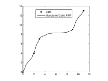
(a): Monotonic rational cubic FIF $S_{1}$

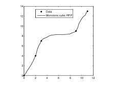
(b): Monotonic rational cubic FIF $S_{2}$ (effect of $\alpha_{1}$)

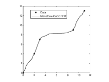
(c): Monotonic rational cubic FIF $S_{3}$ (effect of $\alpha_{2}$)

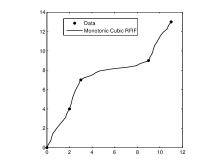
(d): Monotonic rational cubic FIF $S_{4}$ (effect of $r_{3}$)

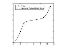
(e): Classical Monotonic rational cubic spline $S_{5}$

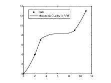
(f): Monotonic rational quadratic FIF $S_{6}$

Figure 1: Monotonic rational cubic/quadratic spline FIFs: $S_{i}$, $i=1,2,\dots,6$.

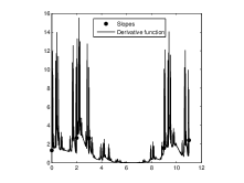
(a): Fractal function $S_{1}^{(1)}$

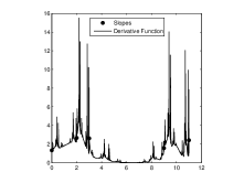
(b): Fractal function $S_{2}^{(1)}$

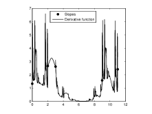
(c): Fractal function $S_{3}^{(1)}$ (smooth in $[2,3]$)

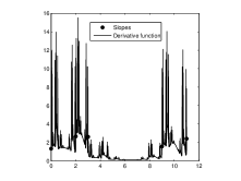
(d): Fractal function $S_{4}^{(1)}$

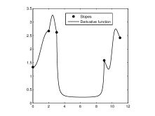
(e): Function $S_{5}^{(1)}$

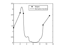
(f): Function $S_{6}^{(1)}$

Figure 2: Derivatives of monotonic rational FIFs in Figs. 1(a)-1(f)

6.2 Convexity Preserving Rational FIFs

Consider the convex data set $\{(2.2,2),(4,0.625),(5,0.4),(10,1),(10.22,1.8)\}$. We computationally generate convex rational cubic spline FIFs by using (3.3) and the parameter values given by Theorem 4.2. The derivative parameters required for the implementation of the IFS scheme are estimated using the arithmetic mean method. The convex rational cubic spline FIF generated in Fig. 3(a) is taken as a reference curve. Changing the scaling factor $\alpha_{3}$ to $0.005$ and keeping the values of the other parameters as in Fig. 3(a) (see Table 2), we obtain the convex rational cubic spline FIF in Fig. 3(b). It can be observed that the change in $\alpha_{3}$ influence the curve only in $[x_{3},x_{4}]$. Further, due to a small value of the scaling factor and a large value of the shape parameter the FIF converges to a line segment in $[x_{3},x_{4}]$, demonstrating the tension effect. Similar experiments may be conducted by changing the scalings in other subintervals and the shape parameters. By taking all the scaling factors to be zero and the shape parameters according to (4.21), a classical rational quadratic spline that retain the data convexity is obtained in Fig. 3(c). Thus, Fig. 3(c) provides a numerical example for the convex rational quadratic spline by Delbourgo [16]. As in the monotonicity case, it can be observed by plotting the graph of the derivatives that the scaling factors provide fractality in the derivatives $S^{(1)}$ or $S^{(2)}$ (more precisely right hand second derivative).

Table 2: Parameters corresponding to the convex rational cubic FIFs

Figure No	Choice of parameters
	$\alpha_{i}$	$0.02$	$0.001$	$0.16$	$0.007$
Fig. 3(a)	$r_{i}$	$37$	$8$	$269$	$8$
	$\alpha_{i}$	$0.02$	$0.001$	$0.005$	$0.007$
Fig. 3(b)	$r_{i}$	$37$	$8$	$269$	$8$
	$\alpha_{i}$	$0$	$0$	$0$	$0$
Fig. 3(c)	$r_{i}$	$3$	$2.6459$	$12.8069$	$3$

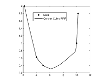
(a): Convex rational cubic FIF

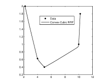
(b): Convex rational cubic FIF (effect of $\alpha_{3}$)

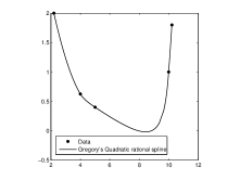
(c): Classical convex rational quadratic spline

Figure 3: Convex rational cubic/quadratic spline FIFs.

6.3 FIFs with Mixed Shape Properties

The theoretical discussion we had in section 6 was confined to data with same shape characteristics in the entire interpolation interval. However, we can also apply our schemes with proper modification and mixing to obtain fractal interpolants for data with mixed shape properties. We illustrate this with two examples.
The first example taken from [32] is a data set generated from a function $\Phi_{1}$ defined on $[0,4]$ which is positive on $[0,1]$, strictly increasing on $[1,2]$, constant on $[2,3]$, and concave on $[3,4]$. Suppose that we want to use the proposed fractal interpolation scheme to construct a $\mathcal{C}^{1}$ approximant to this function interpolating the data set $\{(0,1),(0.5,0.2),(1,1),(1.5,1.3),(2,1.8),(2.5,1.8),\\ (3,1.8),(3.5,1.5),(4,0)\}$ with the same shape characteristics. To achieve this, derivative values that are consistent with the required shapes are estimated: $d_{1}=-3.2$, $d_{2}=d_{5}=d_{6}=d_{7}=0$, $d_{3}=1.1$, $d_{4}=0.8$, $d_{8}=-1.8$, and $d_{9}=-4.2$. We divide the interval into four subintervals of unit length such that in each of the subinterval data possess the same shape property. To obtain a positive rational cubic spline FIF $S_{1}$ in $[0,1]$, we iterate the functional equation (3.3) with the scaling factors and the shape parameters satisfying the required conditions (see Section 5 (i)). Our specific choices of the scaling parameters and the shape parameters are: $\alpha_{1}=\alpha_{2}=0.15$; $r_{1}=1.5$, $r_{2}=0.5$. On the interval $[1,2]$, we apply our monotonicity preserving algorithm with the parameter values $\alpha_{1}=\alpha_{2}=0.3$, $r_{1}=8$, and $r_{2}=1$ to obtain the monotonic rational cubic spline FIF $S_{2}$. Note that here the parameters are indexed by considering the interpolation to take place in the subinterval $[1,2]$, not the entire interval. Following Remark (4.1), we generate a linear interpolant $S_{3}$ on $[2,3]$. Finally, the concavity preserving rational cubic spline FIF $S_{4}$ is obtained on $[3,4]$ by iterating functional equation (3.3) with parameters values satisfying concavity condition, our specific choices being $\alpha_{1}=0.15$, $\alpha_{2}=0.2$, $r_{1}=9$, and $r_{4}=4$. Since the data satisfy both the monotonic decreasing condition and the strictly concave condition on $[3,4]$, and derivative parameters are selected accordingly, the concave interpolation scheme automatically render a concave and monotonically decreasing interpolant (see Section 4.3). The fractal function $S$ on $[1,4]$ (see Fig. 4(a)) is obtained by pasting $S_{i}$, $i=1,2,3,4$. Since $S_{i}$ and $S_{i}^{(1)}$ ($i=1,2,3,4$) are continuous, the continuity of $S$ and $S^{(1)}$ follows from the pasting lemma. Consequently, the fractal function $S\in\mathcal{C}^{1}[0,4]$ given in Fig. 4(a) provides an approximation to $\Phi_{1}$ satisfying the required shape properties.
Consider a function $\Phi_{2}$ defined on $[0,10]$, which is monotonic decreasing on $[0,4]$, monotonic increasing on $[4,6]$, and monotonic decreasing on $[6,10]$. Our second example is concerned with the construction of a $\mathcal{C}^{1}$-approximation which is co-monotone with this function, where all we know about the function is the function values at specified points, say, $\{(0,10),(1.5,5),(4,3.5),\\ (6,7.1),(8,3),(10,0)\}$. As discussed in section 5, we divide the interval in to three subintervals $I_{1}=[0,4]$, $I_{2}=[4,6]$, and $I_{3}=[6,10]$ where the data are monotonic decreasing, monotonic increasing, and monotonic decreasing respectively. Since the interval $I_{2}=[4,6]$ contains only two knot points, the FIF scheme demands insertion of a node in this interval. Let the new node be $(5,6)$. Derivative values that are consistent with the required shapes are chosen as $d_{1}=-4.35$, $d_{2}=-2.31$, $d_{3}=0$, $d_{4}=1.8$ (at the inserted knot), $d_{5}=0$, $d_{6}=-1.77$, and $d_{7}=-1.2$. A rational cubic spline FIF $S_{1}$ is constructed on $I_{1}$ by taking $\alpha_{1}=\alpha_{2}=0.2$, $r_{1}=2$, $r_{2}=12$, and iterating the functional equation (3.3). On $I_{2}$, the functional equation (3.3) with the parameter values $\alpha_{1}=\alpha_{2}=0.3$, $r_{1}=2$, and $r_{2}=91$ generates $S_{2}$. Finally iterations of (3.3) with $\alpha_{1}=\alpha_{2}=0.4$, $r_{1}=2$, and $r_{2}=26$ yield $S_{3}$. The fractal function $S\in\mathcal{C}^{1}$ defined in a piecewise manner by $S\big{|}_{I_{i}}=S_{i}$, $i=1,2,3$ is co-monotone with $\Phi_{2}$, and it is given in Fig. 4(b).

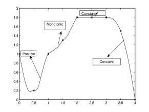
(a): Rational cubic spline FIF with mixed shape property

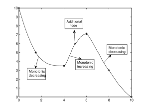
(b): Co-monotone rational cubic FIF

Figure 4: Rational cubic spline FIFs with mixed shape properties.

7 Conclusions

A new kind of rational cubic fractal splines involving shape parameters is proposed in the present work to provide a tool for univariate shape preserving interpolation. Number of parameters in the rational IFS is kept to be minimum (one family of parameters for controlling fractality in the derivative function and one for providing shape preserving characteristics) for computational efficiency. Due to the presence of the scaling factors and the shape parameters involved in the definition, the proposed $\mathcal{C}^{1}$-rational cubic spine FIF generalizes the classical rational splines studied in the references [25, 19, 16]. Despite the implicit and recursive nature of the FIFs, it is shown that the existence of range restricted fractal interpolants depends only on the solvability of a finite set of inequalities resulting from the constraints. These inequalities are shown to be solvable if the shape parameters are above and the scaling factors are below certain explicitly calculable bounds. Uniform convergence of the rational cubic spline FIF to the original data generating function $f\in$ $\mathcal{C}^{4}(I)$ is established. The convergence analysis shows that $O(h^{r})(r=1,2,3,4)$ error bounds can be achieved by suitable choices of the derivatives, the scaling factors, and the shape parameters. Thus, the present interpolation method has convergence properties similar to that of its classical counterpart, which should be considered along with the flexibility and diversity offered by the new method. The scaling factors and the shape parameters can be selected suitably to find an interpolant satisfying chosen properties such as smoothness, approximation order, locality, fractality in the derivative, and shape preservation of the data. The fairness (visual pleasantness) of the interpolant can be achieved through a constrained non-linear optimization. For the shape preserving interpolants with varying irregularity in the derivatives, the result is encouraging for the fractal spline class treated in this paper. Consequently, it is felt that the proposed scheme can provide an efficient mathematical tool for the simulation of curves occurring in the study of physical systems, for instance, in the study of nonlinear control problems such as pendulum-cart system and in some fluid dynamics problems such as motion of a falling sphere in a non-Newtonian fluid.

ACKNOWLEDGEMENTS. The first author is thankful to the SERC DST Project No. SR/S4/MS: 694/10 for this work. The second author is partially supported by the Council of Scientific and Industrial Research India, Grant No. 09/084(0531)/2010-EMR-I.

References

- [1] M. F. BARNSLEY, Fractal functions and interpolations, Constr. Approx., 2(1986), pp. 303-329.
- [2] M. F. BARNSLEY, Fractals Everywhere, Academic Press, Orlando, Florida, 1988.
- [3] M. F. BARNSLEY, J. ELTON, D. HARDIN AND P. MASSOPUST, Hidden variable fractal interpolation functions, SIAM J. Math. Ana., 20(5)(1989), pp. 1218-1242.
- [4] M. F. BARNSLEY AND A. N. HARRINGTON, The calculus of fractal interpolation functions, J. Approx. Theory, 57(1989), pp. 14-34.
- [5] L. D. BERKOVITZ, Convexity and Optimization in , John Wiley & Sons, New York, 2002.
- [6] W. BOEHM, G. FARIN AND J. KAHMANN, A Survey of curve and surface methods in CAGD, CAGD, 1(1984), pp. 1-60.
- [7] A. K. B. CHAND AND G. P. KAPOOR, Generalized cubic spline fractal interpolation functions, SIAM J. Numer. Anal., 44 (2006), pp. 655-676.
- [8] A. K. B. CHAND AND G. P. KAPOOR, Cubic spline coalescence fractal interpolation through moments, Fractals 15(1)(2007), pp. 41-53.
- [9] A. K. B. CHAND AND G. P. KAPOOR, Smoothness analysis of coalescence hidden variable fractal interpolation functions, Int. J. Nonlinear Science, 3(1)(2007), pp. 15-26
- [10] A. K. B. CHAND AND M. A. NAVASCUÉS, Generalized Hermite fractal interpolation, Rev. Real Academic de ciencias. Zaragoza, 64 (2009), pp. 107-120.
- [11] A. K. B. CHAND AND P. VISWANATHAN, Cubic Hermite and cubic spline fractal interpolation functions, AIP Conference Proceedings, 1479(2012), pp. 1467-1470.
- [12] S. CHEN, The non-differentiability of a class of fractal interpolation functions, Acta Math. Sci., 19(4), (1999), pp. 425-430.
- [13] J. C. CLEMENT, Convexity preserving piecewise rational cubic interpolation, SIAM J. Numer. Anal., 27 (1990), pp. 1016-1023.
- [14] P. COSTANTINI AND C. MANNI, Curve and surface construction using Hermite subdivision schemes, J. Comp. Appl. Math., 233(2010), pp. 1660-1673.
- [15] L. DALLA, V. DRAKOPOULOS AND M. PRODROMOU, On the box dimension for a class of nonaffine fractal interpolation functions, Anal. Theory Appl., 19(2003), pp. 220-233.
- [16] R. DELBOURGO, Shape preserving interpolation to convex data by rational functions with quadratic numerator and linear denominator, IMA J. Numer. Anal., 9(1989), pp. 123-126.
- [17] R. DELBOURGO AND J. A. GREGORY, Determination of derivative parameters for a monotonic rational quadratic interpolant, IMA J. Numer. Anal., 5(1985), pp. 397-406.
- [18] R. DELBOURGO AND J. A. GREGORY, rational quadratic spline interpolation to monotonic data, IMA J. Numer. Anal., 3(1983), pp. 141-152.
- [19] R. DELBOURGO AND J. A. GREGORY, Shape preserving piecewise rational interpolation, SIAM J. Sci. Stat. Comput., 6(1985), pp. 967-976
- [20] N. DYN, D. LEVIN AND D. LIU, Interpolatory convexity preserving subdivision schemes for curves and surfaces, Comput. Aided Design, 24(4)(1992), pp. 211-216.
- [21] J. C. FIOROT AND J. TABKA, Shape-preserving cubic polynomial interpolating splines, Math. Comp., 57(1991), pp. 291-298.
- [22] F. N. FRITSCH AND J. BUTLAND, A method for constructing local monotone piecewise cubic interpolants, SIAM J. Sci. Stat. Comput., 5(1984), pp. 303-304.
- [23] F. N. FRITSCH AND R. E. CARLSON, Monotone piecewise cubic interpolation, SIAM J. Numer. Anal., 17(1980), pp. 238-246.
- [24] J. A. GREGORY, Shape preserving spline interpolation, CAGD, 18(1986), pp. 53-57.
- [25] J. A. GREGORY AND R. DELBOURGO, Piecewise rational quadratic interpolation to monotonic data, IMA J. Numer. Anal., 2(1982), pp. 123-130.
- [26] J. A. GREGORY AND M. SARFRAZ, A rational cubic spline with tension, CAGD, 7(1990), pp. 1-13.
- [27] X. HAN, Convexity preserving piecewise rational quartic interpolation, SIAM J. Numer. Anal., 46(2008), pp. 920-929.
- [28] A. JAYARAMAN AND A. BELMONTE, Oscillations of a solid sphere falling through a wormlike micellar fluid, Phys. Rev., 67(2003), 65301.
- [29] W. J. KAMMERER, Polynomial approximations to finitely oscillating functions, Math. Comp. 15(1961), pp. 115-119.
- [30] L. I. LEVKOVICH-MASLYUK, Wavelet-based determination of generating matrices for fractal interpolation functions, Regul. Chaotic Dyn., 3(1998), pp. 20-29.
- [31] E. LUTTON, J. LEVY-VEHEL, G. CRETIN, P. GLEVAREC, AND C. ROLL, Mixed IFS: resolution of the inverse problem using genetic programming, Complex systems, 9(1995), pp. 375-398.
- [32] T. LYCHE AND J. L. MERRIEN, Interpolatory subdivision with shape constraints for curves, Siam J. Numer. Anal., 44(2006) pp. 1095-1121.
- [33] C. MANNI AND P. SABLONNIÉRE, Monotone interpolation of order 3 by cubic splines, IMA J. Numer. Math., 71(1991), pp. 237-252.
- [34] M. A. NAVASCUÉS, Fractal polynomial interpolation, Z. Anal. Anwend, 25(2005), pp. 401-418.
- [35] M. A. NAVASCUÉS AND M. V. SEBASTIÁN, Generalization of Hermite functions by fractal interpolation, J. Approx. Theory, 131(1)(2004), pp. 19-29.
- [36] M. A. NAVASCUÉS AND M. V. SEBASTIÁN, A relation between fractal dimension and Fourier transform -electroencephalographic study using spectral and fractal parameters, Int. J. Comp. Math., 85(2008), pp. 657-665
- [37] M. SARFRAZ, M. Z. HUSSAIN AND M. HUSSAIN, Shape-preserving curve interpolation, Int. J. comput. Math., 89(2012), pp. 35-53.
- [38] D. G. SCHWEIKERT, An interpolation curve using a spline in tension, J. Math. Phys., 45(1966), pp. 312-317
- [39] J. W. SCHMIDT AND W. HEŚS, An always successful method in univariate convex interpolation, Numer. Math., 71(1995), pp. 237-252.
- [40] L. L. SCHUMAKER, On shape preserving quadratic spline interpolation, SIAM J. Numer. Anal., 20(1983), pp. 854-864.
- [41] W. M. SIEBERT, Circuits, Signals, and Systems, MIT press, Cambridge, 1986.
- [42] W. WOLIBNER, Sur un polynôme d’interpolation, Colloq. Math., 2(1951), pp. 136-137.