Symmetry-based coarse-graining of evolved dynamical networks

Abstract

Networks with a prescribed power-law scaling in the spectrum of the graph Laplacian can be generated by evolutionary optimization. The Laplacian spectrum encodes the dynamical behavior of many important processes. Here, the networks are evolved to exhibit subdiffusive dynamics. Under the additional constraint of degree-regularity, the evolved networks display an abundance of symmetric motifs arranged into loops and long linear segments. Exploiting results from algebraic graph theory on symmetric networks, we find the underlying backbone structures and how they contribute to the spectrum. The resulting coarse-grained networks provide an intuitive view of how the anomalous diffusive properties can be realized in the evolved structures.

1 Introduction

Networks have become a principal tool for the modeling of complex systems in a broad range of scientific fields [1, 2, 3]. In a dynamical network the topology describes the couplings between individual units of a dynamical process [4]. The general underlying question of research on dynamical networks is how the network structure shapes the global dynamical behavior.

An important class of processes on networks are Laplacian dynamics in which the graph Laplacian is the operator of the (linearized) time evolution. The Laplacian spectrum and eigenvectors then describe the overall dynamical behavior. This class comprises many physical processes such as dynamics of Gaussian spring polymers [5], transport processes [6], random walks [7], and synchronization of oscillators [8, 9, 10].

Another dynamical aspect is the evolution of network structure. Many systems change their connectivity structure in the course of time which affects the global dynamical behavior. The time scales of these two processes are often well separated with fast dynamics and slowly responding structural evolution. As an example, think of changes in neuronal activity in a brain on the one hand and the formation of synaptic connections on the other hand. In the opposite case, when dynamics and evolution happen on similar time scales one speaks of coevolutionary or adaptive networks [11]. Since the functionality of a system is often closely associated with dynamical behavior evolutionary forces will drive an evolving dynamical network towards some optimized structure.

The method of network evolution adopts this strategy to find networks with prescribed dynamical properties. Based on rules for mutation and selection together with a “fitness” function measuring the quality of a network structure the evolution explores the configuration space towards optimal structures. Evolutionary optimization of networks was applied successfully in various contexts such as modularity in changing environments [12], Boolean switching dynamics [13, 14, 15, 16, 17, 18], and synchronization of oscillators [19, 20, 21, 22, 23]. It has also been shown that networks can be reconstructed from their Laplacian spectra by evolutionary optimization [24, 25].

Recently, network evolution was applied to generate networks which display subdiffusive dynamics [26]. Here, subdiffusion is specified by the average return probability of a random walker that decays more slowly than in normal diffusion. The return probability is directly related to the spectrum of the graph Laplacian via a Laplace transform. Thus, in contrast to other questions like the synchronizability of oscillators where mainly the smallest eigenvalues contribute [10], here the entire spectrum is important. The evolution algorithm optimizes the spectrum with respect to a prescribed target function, which in this case is a pure power law characterized by the spectral dimension ${d_{\mathrm{s}}}$. For subdiffusive dynamics ${d_{\mathrm{s}}}<2$.

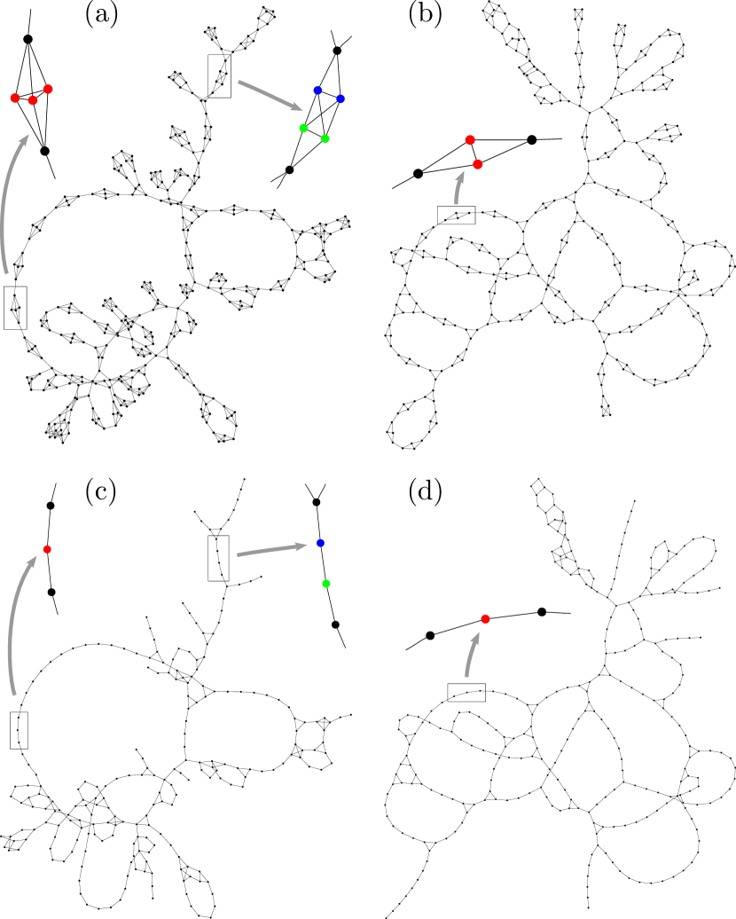
Figure 1: (Color online) Top: Typical $k$-regular network configurations after $10^{6}$ evolution steps towards spectral dimension ${d_{\mathrm{s}}}=1.4$ starting from (a) a square lattice with $k=4$, $N=361$, $M=722$ and (b) a honeycomb lattice with $k=3$, $N=360$, $M=540$. Bottom: The corresponding s-quotients which are of sizes (c) $N=230$, $M=294$ and (d) $N=285$, $M=337$. In the enlarged segments, the colors indicate the orbits to which the respective vertices belong.

To elucidate how the spectral properties are encoded in the structure of the evolved networks, in the present work we apply the method of ref. [26] to regular networks, i.e., networks in which each vertex has the same number of neighbors. Two typical network configurations evolved towards a target spectral dimension of ${d_{\mathrm{s}}}=1.4$ are shown in fig. 1(a) and (b). They exhibit an interesting, modular structure consisting of small symmetric motifs arranged into fractal-like loops and linear segments of different lengths on larger scales. Given that subdiffusive transport is common in comb-like and self-similar structures [27], it is very tempting to attribute the subdiffusive character of the networks to this modular structure. We know, however, that primarily spectral and not structural properties determine the dynamical behavior [8, 28] and that the spectrum of a network can, in general, not be constructed from the spectra of its subnetworks. Nevertheless, in the present case the symmetry of the networks implies that this can be done in a systematic way.

In the following we exploit concepts of algebraic graph theory to extract the large-scale structure of the evolved networks. This is achieved by identifying the symmetries associated with the small-scale motifs and constructing the corresponding quotient network. The quotient graph and in particular the corresponding simple graph represent a systematic coarse-graining of the original networks, and their spectra are considerably closer to the target function of the evolutionary algorithm. To set the stage for this investigation, we begin by providing some background on spectral graph theory and network symmetries.

2 Spectra of dynamical networks

A formal description of a network with $N$ vertices is given by the adjacency matrix $A$. It is an $N\times N$ matrix with elements $A_{ij}=1$ if vertex $i$ is connected with vertex $j$ and $A_{ij}=0$ otherwise. For an undirected network $A$ is symmetric, $A_{ij}=A_{ji}$. In the case of a directed network one has to specify whether $A_{ij}$ describes the presence of the an edge from $i$ to $j$ or vice versa. Both conventions exist in the literature. The graph Laplacian $L$ is another matrix describing the structure of an undirected simple network (no self-loops, no multi-edges). It is defined as $L=D-A$ where $D$ is the diagonal matrix of vertex degrees $k_{i}$, $D_{ij}=k_{i}\delta_{ij}$. The degree $k_{i}=\sum_{j}A_{ij}$ of a vertex $i$ is the number edges incident to the vertex. Note that this operator is sometimes called the algebraic Laplacian to distinguish it from similar operators such as different versions of the normalized Laplacian.

Diffusion processes form a very important class of dynamics. They describe, e.g., how a substance spreads in a medium or an opinion in a society. To be more specific, we consider a process where the flux of some substance along each edge in the network is proportional to the difference in the amount at the end vertices. The time evolution operator of this process on an undirected network is the graph Laplacian. An important global characteristic of such a process is the average probability $P_{0}(t)$ for a random walker to return to its starting point at time $t$. $P_{0}(t)$ is the Laplace transform of the Laplacian eigenvalue density $\rho(\lambda)$, $P_{0}(t)=\int_{0}^{\infty}\mathrm{d}\lambda\exp(-\lambda t)\rho(\lambda)$ [27, 28]. Hence, if the integrated eigenvalue density $I(\lambda)=\int\mathrm{d}\lambda\,\rho(\lambda)$ scales as a power law, $I(\lambda)\propto\lambda^{{d_{\mathrm{s}}}/2}$, then $P_{0}(t)$ decays as a power law, $P_{0}(t)\propto t^{-{d_{\mathrm{s}}}/2}$. The power-law exponent ${d_{\mathrm{s}}}$ is the spectral dimension of the network. For regular lattices, it coincides with the Euclidean dimension [29].

Since the quotient graph to be constructed below is directed, we need to generalize the graph Laplacian to directed networks. For this purpose we consider a diffusion process on a directed network, possibly containing multi-edges and self-loops. Let $x_{i}$ describe the amount of the diffusing quantity on vertex $i$. The flux of this quantity along each outgoing edge should be proportional to $x_{i}$. Then $x_{i}$ decreases at rate $cx_{i}$ for each outgoing edge $i\to j$, and increases at rate $cx_{j}$ for each incoming edge $j\to i$ where $c$ is a diffusion coefficient. Following the convention that $A_{ij}$ is given by the number of directed edges from $i$ to $j$ this yields the set of coupled differential equations

$$\dot{x}_{i} =\sum_{j}A_{ji}cx_{j}-\sum_{j}A_{ij}cx_{i}=c\sum_{j}A_{ji}x_{j}-cx_{i}k_{i}^{\mathrm{out}}$$

$$=c\sum_{j}\left(A_{ji}-\delta_{ji}k_{j}^{\mathrm{out}}\right)x_{j}=-c\sum_{j}L_{ji}^{\mathrm{out}}x_{j}$$ (1)

where $k_{i}^{\mathrm{out}}=\sum_{j}A_{ij}$ denotes the out-degree of vertex $i$ and

$$L_{ji}^{\mathrm{out}}=k_{j}^{\mathrm{out}}\delta_{ji}-A_{ji}$$ (2)

are the elements of the out-degree Laplacian. So, when considering diffusion processes on a network the out-degree Laplacian is the correct generalization of the graph Laplacian as time evolution operator to directed networks.

3 Symmetries in networks

In a symmetric network, the spectrum and, correspondingly, the set of eigenvectors can be split into two classes. Some of the eigenpairs stem from the symmetric motifs and are inherited by the network as a whole while the remaining ones are the eigenpairs of the underlying backbone structure, the quotient network. In order to make this statement more precise and formally tractable we first summarize some basic notions on the mathematical description of network symmetry. More details, exact definitions, and proofs can be found in ref. [30, 31].

The symmetry of a network $G$ is described by its automorphism group $\mathrm{Aut}(G)$. An automorphism is a permutation of vertices which does not change the network structure (preserves the adjacency). A network is called symmetric if it has a non-trivial automorphism group. By a direct product decomposition $\mathrm{Aut}(G)=H_{1}\times H_{2}\times\ldots\times H_{k}$ the automorphism group can be split into geometric factors $H_{i}$ which act independently on the network. A symmetric motif $\mathcal{M}_{H}$ of a network is the induced subgraph on the support of a geometric factor $H$. Intuitively speaking, a symmetric motif $\mathcal{M}_{H}$ is a minimal subgraph whose vertices are moved by $H$.

The action of a network’s automorphism group $\mathrm{Aut}(G)$ partitions the vertex set $V$ into disjoint equivalence classes called orbits. The orbit of a vertex $v\in V$ is the set of vertices $\Delta(v)\subset V$ to which $v$ maps under the action of $\mathrm{Aut}(G)$,

$$\Delta(v)=\{gv\in V\,|\,g\in\mathrm{Aut}(G)\}\,.$$ (3)

In the enlarged parts of fig. 1(a) and (b) examples of how the vertices in a symmetric motif are grouped into orbits are indicated by their colors. In general, it may, however, be necessary to swap a larger fraction of a network in order to map two vertices in the same orbit onto each other without altering the adjacency. Nevertheless all vertices in the same orbit are structurally equivalent (perform the same function in the network).

The quotient graph is a network coarse-graining based on this structural equivalence. The set of vertices of the quotient $Q=G/\mathbf{\Delta}$ is given by the orbits $\mathbf{\Delta}=\{\Delta_{1},\Delta_{2},\ldots,\Delta_{r}\}$ of the network $G$. Note that due to the structural equivalence the number of neighbors in $\Delta_{y}$ of a vertex $v\in\Delta_{x}$, called $q_{xy}$, does not depend on the choice of $v$ but only on $x$ and $y$. A partition with this property is called equitable which has important consequences for the relation between the spectra of $G$ and $Q$ (see below). The quotient graph $Q$ of a network $G$ has vertex set $\mathbf{\Delta}$ and adjacency matrix $\{q_{xy}\}_{x,y=1,\ldots,r}$. It is by definition directed and generally contains multi-edges and self-loops. If one is working with simple networks this may be inconvenient. As a further simplification the s-quotient $Q_{\mathrm{s}}$ is defined as the underlying simple graph of the quotient. It already captures essential properties such as the size and adjacency of the quotient. Fig. 1(c) and (d) show the s-quotients of the two networks above. The colored vertices in the enlarged segments indicate the corresponding orbits in the parent networks.

A key result from algebraic graph theory [31] relates the adjacency spectra and eigenvectors of a network $G$ and its quotient graph $Q$ (or, in general, any quotient $G/\pi$ from an equitable partition $\pi$). All eigenvalues of the quotient are also eigenvalues of the parent network. Moreover, to each eigenpair $(\lambda,\mathbf{v}=(v_{1},\ldots,v_{m}))$ of $Q$ there exists an eigenpair $(\lambda,\mathbf{\bar{v}}=(\bar{v}_{1},\ldots,\bar{v}_{n}))$ of $G$ with $\bar{v}_{i}=v_{x}$ for all $i\in\Delta_{x}$ (eigenvectors are constant $v_{x}$ on each orbit $\Delta_{x}$). These eigenvectors are called lifted from the eigenvectors of the quotient. The remaining eigenpairs of $G$ are constructed from the redundant eigenpairs of the symmetric motifs of $G$: If $(\lambda,\mathbf{v}=(v_{1},\ldots,v_{k}))$ is an eigenpair of the symmetric motif $\mathcal{M}$—isolated from the rest of the network—which is redundant (i.e. $\sum_{i\in\Delta}v_{i}=0$ for each orbit $\Delta\in\mathcal{M}$) then $(\lambda,\mathbf{\hat{v}})$ is an eigenpair of $G$ with $\hat{v}_{i}=v_{i}$ for all $i\in\mathcal{M}$ and $\hat{v}_{i}=0$ for $i\notin\mathcal{M}$ (eigenvectors are localized on the symmetric motifs).

To summarize, the adjacency eigenpairs of a symmetric network $G$ fall into two classes. (1) The eigenpairs of the quotient of $G$ are also eigenpairs of $G$ with constant values of the eigenvectors on the orbits. (2) The redundant eigenpairs of the symmetric motifs of $G$ are also eigenpairs of $G$ with eigenvectors localized on the respective motif.

All these statements for the adjacency spectrum and eigenvectors are elaborated and proven in ref. [30]. In the appendix we show that they also hold for the Laplacian spectrum and eigenvectors.

For practical computations of automorphism groups efficient and easily applicable algorithms are available such as the nauty program [32] which was used in this study to find orbits and construct network quotients.

4 Application to regular evolved networks

In ref. [26] the method of network evolution was applied to construct networks with a given non-trivial spectral dimension $d_{\mathrm{s}}$. The algorithm searches the configuration space of connected networks with a given size for network structures which resemble the power law in the Laplacian spectrum as closely as possible. The introduced distance measure $\mathcal{D}$ (called $\Delta$ in ref. [26]) is defined as the integral over the squared difference between integrated eigenvalue densities. In contrast to other proposed spectral distances [33] it can be applied to compare the spectrum with a general function as well as with other spectra. However, since $\mathcal{D}$ inherently depends on the number of vertices, networks of different sizes cannot be compared directly. The most simple rules for mutation and selection were applied, namely a random movement of a single edge and the acceptance of a proposed move if $\mathcal{D}$ decreases and the whole network remains connected. Starting from regular lattices and random graphs networks were successfully evolved under the constraints of a fixed number of vertices and a fixed average degree.

An even stricter condition is to fix the individual degree of each vertex, as for example in a $k$-regular network where all vertices have the same degree $k$. Is it—under this additional constraint—still possible to construct networks with a given non-trivial value of the spectral dimension $d_{\mathrm{s}}$? To answer this question we applied the network evolution algorithm starting from square lattices ($k=4$) and honeycomb lattices ($k=3$) and corresponding $4$- and $3$-regular random networks. As in the preceding study [26] it turns out that the evolution does not depend on the two choices (lattice or random network) of initial conditions. The conservation of the degree sequence (or the individual degree of each node) in the course of the evolution can be realized by an “edge-crossing” update. In each evolution step two edges $v_{1}$–$v_{2}$ and $v_{3}$–$v_{4}$ are randomly chosen and “crossed” to $v_{1}$–$v_{4}$ and $v_{3}$–$v_{2}$. When the edges are drawn one has to make sure that the four vertices $v_{1},v_{2},v_{3},v_{4}$ are all distinct and that the edges $v_{1}$–$v_{4}$ and $v_{3}$–$v_{2}$ do not exist before the update.

The evolutions were run for $10^{6}$ time steps towards a target value of the spectral dimension of $d_{\mathrm{s}}=1.4$. Typical network configurations at the end of the evolutions of $3$- and $4$-regular networks are shown in fig. 1(a) and (b). These networks appear to have similar large-scale structures of long loops built up by very frequently appearing symmetric motifs on small scales.

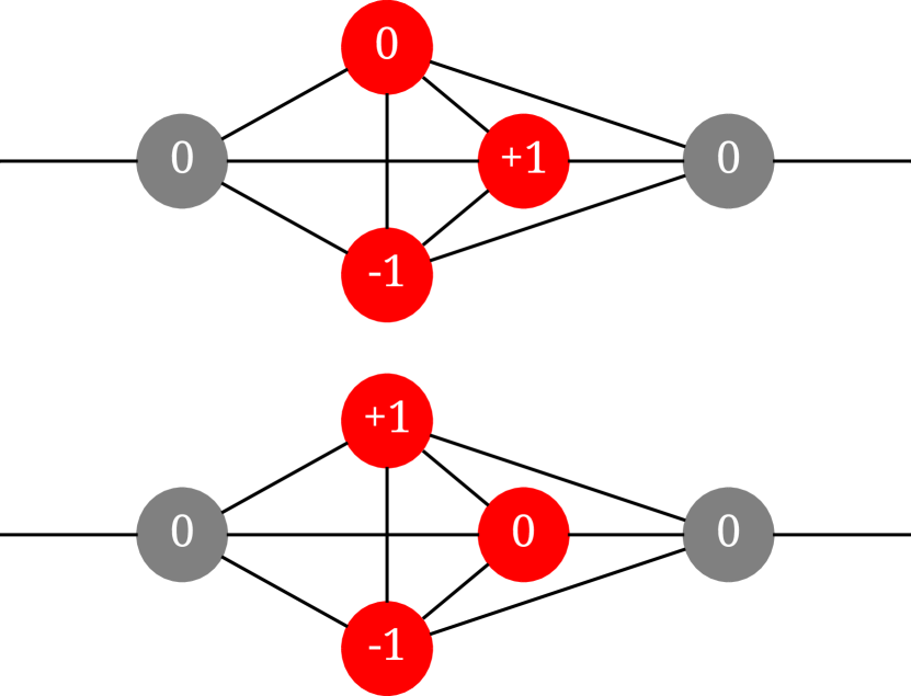
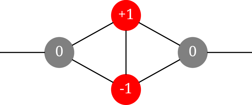
Figure 2: (Color online) Redundant Laplacian eigenvectors of the most prominent motifs in 4-regular (left) and 3-regular (right) evolved networks as depicted in fig. 1(a) and (b). The symmetric vertices are colored red. The corresponding eigenvalues are $\{5,5\}$ (left) and $\{4\}$ (right).

The most abundant of these motifs are shown in fig. 2. They consist of a complete subnetwork of $k-1$ vertices, each of which is joined to two boundary vertices connecting to the rest of the network. The vertices are labeled by their redundant Laplacian eigenvectors and the corresponding eigenvalues are $\{5,5\}$ in the 4-regular and $\{4\}$ in the 3-regular case. These are also eigenvalues of the network as a whole, which explains the high degeneracy giving rise to the large step in the integrated eigenvalue density in fig. 3. The motifs are assembled to form large-scale structures with long loops which appear to be quite similar in both cases.

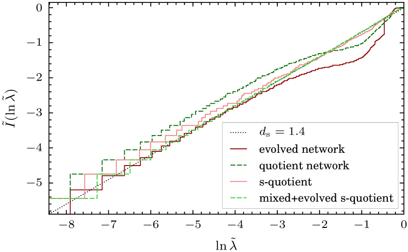
Figure 3: (Color online) Logarithmically integrated Laplacian eigenvalue densities of the 4-regular evolved network from fig. 1(a) and its quotient, s-quotient (fig. 1(c)) and an evolved network of the same size (number of vertices and number of edges) as the s-quotient. The eigenvalue density is plotted as a function of $\ln\tilde{\lambda}$, where $\tilde{\lambda}=\lambda/\lambda_{\mathrm{max}}\leq 1$ is the eigenvalue normalized by the largest eigenvalue of the network [26]. The black dotted line indicates the target integrated density with ${d_{\mathrm{s}}}=1.4$.

The large-scale structures of these networks become more evident in their s-quotients depicted in fig. 1(c) and (d). One can clearly see the arrangement of loops of different lengths. Seen as a coarse-graining transformation, the s-quotient on average reduces the network sizes from $N=361$ vertices and $M=722$ edges to $N\approx 229(6)$ and $M\approx 302(17)$ for 4-regular parent networks and from $N=360$, $M=540$ to $N\approx 281(6)$, $M\approx 330(9)$ for 3-regular parent networks (standard deviations in parentheses).

How to assess the quality of the s-quotients with respect to the optimization goal of the evolution? The ultimate goal of the evolution algorithm is to construct networks with a Laplacian spectrum which resembles the power law $I(\lambda)\propto\lambda^{d_{\mathrm{s}}/2}$. Figure 3 displays the spectra—as logarithmically integrated densities $\tilde{I}(\ln\tilde{\lambda})$ (see eq. (5) of ref. [26] for the exact definition)—for an exemplary 4-regular evolved network, its quotient, s-quotient, and an evolved network of the same size as the s-quotient (“mixed and evolved s-quotient”). The latter class of networks was analyzed in order to get an idea of how the quotients and s-quotients compare to unconstrained evolved networks of the same size. They are constructed by optimizing networks of the same size (same numbers of vertices and edges) by means of the unrestricted version of the evolution algorithm (conserving these numbers and the connectedness only). Technically, since the s-quotients are very sparse networks, instead of generating random networks, the edges of the s-quotients are randomized (keeping the whole network connected) and then the evolution is run.

As predicted by theory, the spectrum of the quotient resembles the spectrum of its parent up to the highly degenerate redundant eigenvalues of the symmetric motifs. By removing the corresponding steps in the integrated eigenvalue density the fit to the target spectrum is improved in the regime of large eigenvalues, whereas the region of small $\lambda$ is unaffected. In contrast, there is no rigorous relation between the spectra of the parent network and the s-quotient. Therefore it was not to be expected that the spectrum of the s-quotient resembles the power law even more closely, as seen in the figure. In terms of the average distance measure $\bar{\mathcal{D}}$ estimated from $100$ realizations of the evolution, the quotients have a value of $\bar{\mathcal{D}}=0.09(1)$ which is reduced by a factor of three in the s-quotients ($\bar{\mathcal{D}}=0.03(2)$). Nevertheless, the unconstrained evolution of networks of the same size succeeds in finding networks with a spectrum even closer to the desired power law, reaching an average value of $\bar{\mathcal{D}}=0.0045(1)$. However, similar to the networks obtained in ref. [26], the networks resulting from the unconstrained evolution algorithm cannot be easily spread out and visualized in a plane.

Figure 4: (a) Typical $3$-regular network configuration after $10^{6}$ evolution steps towards ${d_{\mathrm{s}}}=1.1$ starting from a honeycomb lattice with $N=360$, $M=540$ and (b) corresponding s-quotient, $N=260$, $M=263$.

What happens for a more extreme evolution target? Since the evolution runs were started from two-dimensional lattices it should be more difficult to find networks with a spectral dimension closer to $1$. Fig. 4 shows a typical network configuration from an evolution towards ${d_{\mathrm{s}}}=1.1$ together with the corresponding s-quotient. In this case, the basic motifs are arranged to form even longer linear chains instead of loops resulting in an almost one-dimensional s-quotient.

An important question is why the evolved networks assume the observed shape of symmetric motifs assembled in loops and linear chains (see fig. 1(a) and (b) and 4(a)). A possible explanation is that they have too many edges to form structures with a low spectral dimension. The formation of the symmetric motifs makes it possible to “hide” the excess edges in the motifs and form large-scale structures with the desired scaling in the small Laplacian eigenvalues. Additionally, the motifs may effectively act as particle traps and thus slow down the diffusion process. The formation of loops and linear chains on larger scales is brought out more clearly in the coarse-grained s-quotients in fig. 1(c) and (d) and 4(b) where the symmetric motifs are removed.

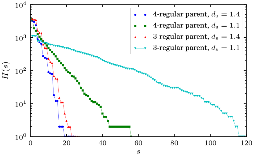
Figure 5: (Color online) Histogram of linear segment lengths $s$ in s-quotients from 4-regular and 3-regular evolved networks for different target spectral dimensions ${d_{\mathrm{s}}}$. Shown are cumulative histograms $H(s)=\int_{s}^{\infty}h(t)\,\mathrm{d}t$ of the absolute frequencies $h(s)$ for $100$ realizations of each.

As a first approach towards quantifying the loop structure we analyzed the lengths of linear segments (connected maximal subgraphs of nodes with a maximum degree two) in the s-quotients in fig. 5. We observe a very broad distribution in this quantity. However, the networks appear to be too small for a systematic scaling analysis.

5 Conclusions

We presented and analyzed subdiffusive networks found by evolutionary optimization. Subdiffusion is known to be observed in various network structures such as regular fractals, percolation clusters or combs with power-law distributed teeth lengths [27]. In the latter, the delay is caused by the time a random walker spends on the teeth of the comb. In the networks presented here, we observe backbone structures with loops and dangling ends of different length scales which seem to be the main source of subdiffusive behavior. The networks are, however, too small for a quantitative analysis of the distribution of these lengths. A more in-depth study on this question would be an interesting continuation of this work.

6 Appendix

We show that the relations between adjacency spectra and eigenvectors of a network $G$ on the one hand and its quotient $Q$ and symmetric motifs on the other hand also hold for the Laplacian spectrum and eigenvectors. The reasoning is the same as in Appendix A of ref. [30]. First, recall that the characteristic matrix $P$ of the equitable partition $\pi=\{C_{1},\ldots,C_{r}\}$ is defined by $P_{ix}=1$ if vertex $i\in C_{x}$ and $P_{ix}=0$ otherwise. It remains to prove that the space $W$ spanned by the column vectors of $P$ is also $L$-invariant. For this, $W$ is $L$-invariant ($Lu\in W$ for all $u\in W$) if and only if there exists a matrix $\tilde{L}$ such that

$$LP=P\tilde{L}\,.$$ (4)

$\tilde{L}$ is then the graph Laplacian of the quotient network $Q=G/\pi$. Let $B$ ($B_{xy}=q_{xy}$ for the orbit partition above) be the adjacency matrix of the quotient. Define $\tilde{L}=\tilde{D}-B$ with $\tilde{D}_{xy}=\tilde{k}_{x}\delta_{xy}$ and $\tilde{k}_{x}=\sum_{y}B_{xy}$. Since $AP=PB$ it remains to show that $DP=P\tilde{D}$. The left hand side reads

$$(DP)_{ix}=\sum_{j}D_{ij}P_{jx}=\sum_{j}k_{i}\delta_{ij}P_{jx}=k_{i}P_{ix}$$ (5)

which is the degree of vertex $i$ if $i\in C_{x}$ and zero otherwise. The right hand side reads

$$(P\tilde{D})_{ix} =\sum_{y}P_{iy}\tilde{D}_{yx}=\sum_{y}P_{iy}\tilde{k}_{y}\delta_{yx}$$

$$=P_{ix}\tilde{k}_{x}=P_{ix}\sum_{y}B_{xy}\,.$$ (6)

Since $B_{xy}$ is the number of neighbors in $C_{y}$ of a vertex from $C_{x}$, $\sum_{y}B_{xy}$ gives the total number of neighbors of a vertex in $C_{x}$ and eq. (6) evaluates to the degree of vertex $i$ if it belongs to $C_{x}$ and zero otherwise. This is the same as eq. (5) which completes the proof.

Note that the definition of the Laplacian $\tilde{L}$ of the quotient graph is consistent with the out-degree Laplacian $L^{\mathrm{out}}$ defined in eq. (2). In particular, the definition of $q_{xy}$ corresponds to the convention that $A_{ij}$ describes directed edges from $i$ to $j$.

References

- [1] \NameAlbert R. Barabási A.-L. \REVIEWReviews of Modern Physics74200247.
- [2] \NameNewman M. E. J. \REVIEWSIAM Review452003167.
- [3] \NameDorogovtsev S. N., Goltsev A. V. Mendes J. F. F. \REVIEWReviews of Modern Physics8020081275.
- [4] \NameBarrat A., Barthélemy M. Vespignani A. \BookDynamical Processes on Complex Networks (Cambridge University Press, Cambridge) 2008.
- [5] \NameGurtovenko A. Blumen A. \BookGeneralized gaussian structures: Models for polymer systems with complex topologies in \BookPolymer Analysis, Polymer Theory no. 182 in Advances in Polymer Science (Springer, Berlin Heidelberg) 2005 pp. 171–282.
- [6] \NameGallos L. K., Song C., Havlin S. Makse H. A. \REVIEWProc. Natl. Acad. Sci. U.S.A.10420077746 .
- [7] \NameNoh J. D. Rieger H. \REVIEWPhys. Rev. Lett.922004118701.
- [8] \NameAtay F. M., Bıyıkoğlu T. Jost J. \REVIEWPhysica D: Nonlinear Phenomena224200635.
- [9] \NameMotter A. E. \REVIEWNew Journal of Physics92007182.
- [10] \NameArenas A., Díaz-Guilera A., Kurths J., Moreno Y. Zhou C. \REVIEWPhysics Reports469200893.
- [11] \NameGross T. Blasius B. \REVIEWJournal of The Royal Society Interface52008259 .
- [12] \NameKashtan N. Alon U. \REVIEWProc. Natl. Acad. Sci. U.S.A.102200513773 .
- [13] \NameBornholdt S. Rohlf T. \REVIEWPhys. Rev. Lett.8420006114.
- [14] \NameOikonomou P. Cluzel P. \REVIEWNat. Phys.22006532.
- [15] \NameBraunewell S. Bornholdt S. \REVIEWPhysical Review E772008060902(R).
- [16] \NameShao Z. Zhou H. \REVIEWPhysica A3882009523.
- [17] \NameSzejka A. Drossel B. \REVIEWPhysical Review E812010021908.
- [18] \NameGreenbury S. F., Johnston I. G., Smith M. A., Doye J. P. Louis A. A. \REVIEWJ. Theor. Biol.267201048.
- [19] \NameDonetti L., Hurtado P. I. Muñoz M. A. \REVIEWPhys. Rev. Lett.952005188701.
- [20] \NameDonetti L., Neri F. Muñoz M. A. \REVIEWJ. Stat. Mech.: Theory Exp.20062006P08007.
- [21] \NameDonetti L., Hurtado P. I. Muñoz M. A. \REVIEWJ. Phys. A: Math. Theor.412008224008.
- [22] \NameRad A. A., Jalili M. Hasler M. \REVIEWChaos182008037104.
- [23] \NameGorochowski T. E., di Bernardo M. Grierson C. S. \REVIEWPhysical Review E812010056212.
- [24] \NameIpsen M. Mikhailov A. S. \REVIEWPhysical Review E662002046109.
- [25] \NameComellas F. Diaz-Lopez J. \REVIEWPhysica A: Statistical Mechanics and its Applications38720086436.
- [26] \NameKaralus S. Porto M. \REVIEWEPL (Europhysics Letters)99201238002.
- [27] \NameHavlin S. Ben-Avraham D. \REVIEWAdvances in Physics512002187.
- [28] \NameSamukhin A. N., Dorogovtsev S. N. Mendes J. F. F. \REVIEWPhysical Review E772008036115.
- [29] \NameBurioni R. Cassi D. \REVIEWJournal of Physics A: Mathematical and General382005R45.
- [30] \NameMacArthur B. D. Sánchez-García R. J. \REVIEWPhysical Review E802009026117.
- [31] \NameGodsil C. D. Royle G. \BookAlgebraic graph theory no. 207 in Graduate texts in mathematics (Springer, New York) 2004.
- [32] \NameMcKay B. D. Piperno A. \REVIEWJournal of Symbolic Computation60201494.
- [33] \NameJurman G., Visintainer R. Furlanello C. \REVIEWNeural Nets Wirn102262011227.