Cosmic constraint on the unified model of dark sectors with or without a cosmic string fluid in the varying gravitational constant theory

Abstract

Observations indicate that most of the universal matter are invisible and the gravitational constant $G(t)$ maybe depends on the time. A theory of the variational $G$ (VG) is explored in this paper, with naturally producing the useful dark components in universe. We utilize the observational data: lookback time data, model-independent gamma ray bursts, growth function of matter linear perturbations, type Ia supernovae data with systematic errors, CMB and BAO to restrict the unified model (UM) of dark components in VG theory. Using the best-fit values of parameters with the covariance matrix, constraints on the variation of $G$ are $(\frac{G}{G_{0}})_{z=3.5}\simeq 1.0015^{+0.0071}_{-0.0075}$ and $(\frac{\dot{G}}{G})_{today}\simeq-0.7252^{+2.3645}_{-2.3645}\times 10^{-13}yr^{-1}$, the small uncertainties around constants. Limit on the equation of state of dark matter is $w_{0dm}=0.0072^{+0.0170}_{-0.0170}$ with assuming $w_{0de}=-1$ in unified model, and dark energy is $w_{0de}=-0.9986^{+0.0011}_{-0.0011}$ with assuming $w_{0dm}=0$ at prior. Restriction on UM parameters are $B_{s}=0.7442^{+0.0137+0.0262}_{-0.0132-0.0292}$ and $\alpha=0.0002^{+0.0206+0.0441}_{-0.0209-0.0422}$ with $1\sigma$ and $2\sigma$ confidence level. In addition, the effect of a cosmic string fluid on unified model in VG theory are investigated. In this case it is found that the $\Lambda$CDM ($\Omega_{s}=0$, $\beta=0$ and $\alpha=0$) is included in this VG-UM model at $1\sigma$ confidence level, and the larger errors are given: $\Omega_{s}=-0.0106^{+0.0312+0.0582}_{-0.0305-0.0509}$ (dimensionless energy density of cosmic string), $(\frac{G}{G_{0}})_{z=3.5}\simeq 1.0008^{+0.0620}_{-0.0584}$ and $(\frac{\dot{G}}{G})_{today}\simeq-0.3496^{+26.3135}_{-26.3135}\times 10^{-13}yr^{-1}$.

I Introduction

Gravity theories are usually studied with an assumption that Newton gravity constant $G$ is a constant. But some observations hint that $G$ maybe depends on the time VG-t , such as observations from white dwarf star VG-MNRAS-2004-dwarf ; VG-PRD-2004-white , pulsar VG-APJ , supernovae VG-PRD-2002-SN and neutron star VG-PRL-1996-neutron . In addition, cosmic observations predict that about 95% of the universal matter is invisible, including dark matter (DM) and dark energy (DE). The unified models of two unknown dark sectors (DM and DE) have been studied in several theories, e.g. in the standard cosmology UM1 ; UM2 ; UM3 , in the Ho$\check{r}$ava-Lifshitz gravity UM-HL , in the RS UM-RS and the KK higher-dimension gravity UM-KK . In this paper, we study the unified model of dark components in theory of varying gravitational constant (VG). The attractive point of this model is that the variation of $G$ could result to the invisible components in universe, by relating the Lagrangian quantity of the generalized Born-Infeld theory to the VG theory. One source of DM and DE is introduced. In addition, given that cosmic string have been studied in some fields, such as in emergent universe cs-emergent ; cs-emergent1 , in modified gravity cs-modified , in inflation theory cs-inflation , and so on cs-others ; cs-others1 ; cs-others2 ; cs-others3 . Here we discuss the effect of a cosmic string fluid on cosmic parameters in VG theory. Using the Markov Chain Monte Carlo (MCMC) method MCMC , the cosmic constraints on unified model of DM and DE with (or without) a cosmic string fluid are performed in the framework of time-varying gravitational constant. The used cosmic data include the lookback time (LT) data lt-data ; lt-data1 , the model-independent gamma ray bursts (GRBs) data grbs-data , the growth function (GF) of matter linear perturbations fdata1 ; fdata12 ; fdata-add1 ; fdata-add2 ; fdata2 ; fdata3 ; fdata4 ; fdata5 , the type Ia supernovae (SNIa) data with systematic errors sn-scp-data , the cosmic microwave background (CMB) 9ywmap , and the baryon acoustic oscillation (BAO) data including the radial BAO scale measurement bao-radial and the peak-positions measurement BAO-WiggleZ ; BAO-2dFGRs ; BAO-SDSS .

II A time-varying gravitational constant theory with unified dark sectors and a cosmic string fluid

We adopt the Lagrangian quantity of system

$$L=\sqrt{g}\left(\frac{R}{G(t)}+16\pi\mathcal{L}_{u}\right)$$ (1)

with a parameterized time-varying gravitational constant $G=G_{0}a(t)^{-\beta}$. $t$ is the cosmic time, $a=(1+z)^{-1}$ is the cosmic scale factor, and $z$ denotes the cosmic redshift. $g$ is the determinant of metric, $R$ is the Ricci scalar, and $\mathcal{L}_{u}=\mathcal{L}_{b}+\mathcal{L}_{r}+\mathcal{L}_{d}+\mathcal{L}_{s}$ corresponds to the Lagrangian density of universal matter including the visible ingredients: baryon $\mathcal{L}_{b}$ and radiation $\mathcal{L}_{r}$ and the invisible ingredients: dark sectors $\mathcal{L}_{d}$ and cosmic string (CS) fluid $\mathcal{L}_{s}$. Utilizing the variational principle, the gravitational field equation can be derived vg-field ,

$$R_{\mu\nu}-\frac{1}{2}Rg_{\mu\nu}=8\pi GT_{\mu\nu}+G(\nabla_{\mu}\partial_{\nu}G^{-1}-g_{\mu\nu}\nabla_{\sigma}\partial^{\sigma}G^{-1})$$ (2)

in which $R_{\mu\nu}$ is the Ricci tensor, $T_{\mu\nu}$ is the energy-momentum tensor of universal matter that comprise the pressureless baryon ($w_{b}=\frac{p_{b}}{\rho_{b}}=0$), the positive-pressure photon ($w_{r}=\frac{p_{r}}{\rho_{r}}=\frac{1}{3}$) , the CS fluid ($w_{s}=\frac{p_{s}}{\rho_{s}}=-\frac{1}{3}$) and the unknown dark components $(w_{d}=\frac{p_{d}}{\rho_{d}})$. $w$ is the equation of state (EoS), $p$ is the pressure and $\rho$ denotes the energy density, respectively. Taking the covariant divergence for Eq. (2) and utilizing the Bianchi identity result to

$$3H(\frac{\dot{G}}{G})^{2}+3\frac{\ddot{a}}{a}\frac{\dot{G}}{G}+8\pi[\dot{G}\rho+G\dot{\rho}+3HG(\rho+p)]=0$$ (3)

or its equivalent form

$$3H\beta[(\beta-1)H^{2}-\dot{H}]+8\pi G[\dot{\rho}+3H(\rho+p)-\beta H\rho]=0.$$

In the Friedmann-Robertson-Walker geometry, the evolutional equations of universe in VG theory are

$$H^{2}=\frac{8\pi G_{0}}{3}a^{-\beta}\rho-\beta H^{2},$$ (4)

$$2\frac{\ddot{a}}{a}+H^{2}=-8\pi G_{0}a^{-\beta}p-\beta H^{2}-\beta^{2}H^{2}-\beta\frac{\ddot{a}}{a}.$$ (5)

From Eq.(4), we can see that a CS fluid can be equivalent to a curvature term in constant-$G$ theory, while this fluid could not be equivalent to the curvature term in the VG theory due to the term $a^{-\beta}$ multiplying the density. Combing the Eqs. (3), (4) and (5), we have

$$\dot{\rho}+3H(\rho+\frac{2+2\beta}{2+\beta}p)=\frac{\beta-\beta^{2}}{2+\beta}H\rho.$$ (6)

”Dot” represents the derivative with respect to cosmic time $t$. Integrating Eq. (6) can gain the energy density of baryon $\rho_{b}\propto a^{\frac{-\beta^{2}-2\beta-6}{2+\beta}}$, the energy density of radiation $\rho_{r}\propto a^{\frac{-\beta^{2}-4\beta-8}{2+\beta}}$ and the energy density of cosmic string $\rho_{s}\propto a^{\frac{-\beta^{2}-4}{2+\beta}}$. Relative to the constant-$G$ theory, the evolutional equations of energy densities are obviously modified in VG theory for the existence of VG parameter $\beta$.

We concentrate on the Lagrangian density of dark components with the form $\mathcal{L}_{d}=-A^{\frac{1}{1+\alpha}}[1-(V^{{}^{\prime}}(\varphi))^{\frac{1+\alpha}{2\alpha}}]^{\frac{\alpha}{1+\alpha}}$ from the generalized Born-Infeld theory L-UM , in which $V(\varphi)$ is the potential. Relating this scalar field $\varphi$ with the time-varying gravitational constant by $\varphi(t)=G(t)^{-1}$, it is then found that the dark ingredients can be induced by the variation of $G$. The energy density of dark fluid in $VG$ frame complies with

$$\rho_{d}=\rho_{0d}[B_{s}+(1-B_{s})a^{(-3+\frac{\beta-\beta^{2}}{2+\beta})(1+\alpha)}]^{\frac{1}{1+\alpha}},$$ (7)

here parameter $\beta$ reflects the variation of $G$, $\alpha$ and $B_{s}=\frac{6+6\beta}{\beta^{2}+2\beta+6}\frac{A}{\rho_{0VG-GCG}^{1+\alpha}}$ are model parameters. Eq. (7) shows that the behavior of $\rho_{d}$ is like cold DM at early time (for $a\ll 1$, $\rho_{d}\approx\rho_{0d}(1-B_{s})^{\frac{1}{1+\alpha}}a^{-3+\frac{\beta-\beta^{2}}{2+\beta}}$), and like cosmological-constant type DE at late time (for $a\gg 1$, $\rho_{d}\approx\rho_{0d}B_{s}^{\frac{1}{1+\alpha}}$). Then Eq. (7) introduces a unified model (UM) of dark sectors in VG theory (called VG-UM). The Hubble parameter $H$ in the VG-UM model reads

$$H=\sqrt{\frac{H^{2}_{0}}{1+\beta}\{\Omega_{0d}[B_{s}a^{-\beta(1+\alpha)}+(1-B_{s})a^{-(3+\frac{2\beta^{2}+\beta}{2+\beta})(1+\alpha)}]^{\frac{1}{1+\alpha}}+\Omega_{b}a^{\frac{-2\beta^{2}-4\beta-6}{2+\beta}}+\Omega_{r}a^{\frac{-2\beta^{2}-6\beta-8}{2+\beta}}+\Omega_{s}a^{\frac{-2\beta^{2}-2\beta-4}{2+\beta}}\}},$$ (8)

with Hubble constant $H_{0}$ and dimensionless energy densities $\Omega_{b}=\frac{8\pi G_{0}\rho_{0b}}{3H^{2}_{0}}$, $\Omega_{r}=\frac{8\pi G_{0}\rho_{0r}}{3H_{0}^{2}}$, $\Omega_{s}=\frac{8\pi G_{0}\rho_{0s}}{3H^{2}_{0}}$, and $\Omega_{0d}+\Omega_{b}+\Omega_{r}+\Omega_{s}=1+\beta$. For $\beta=0$, bove equations are reduced to the standard forms in the constant-$G$ theory.

III Data fitting

III.1 Lookback Time

Refs. lt-df ; lt-df1 define the LT as the difference between the current age $t_{0}$ of universe at $z=0$ and the age $t_{z}$ of a light ray emitted at $z$,

$$t_{L}(z)=\int_{0}^{z}\frac{dz^{{}^{\prime}}}{(1+z^{{}^{\prime}})H(z^{{}^{\prime}})}.$$ (9)

Then the age $t(z_{i})$ of an object at redshift $z_{i}$ can be expressed by the difference between the age of universe at $z_{i}$ and the age of universe at $z_{F}$ (object was born) lt-data ,

$$t(z_{i})=\int_{z_{i}}^{\infty}\frac{dz^{{}^{\prime}}}{(1+z^{{}^{\prime}})H(z^{{}^{\prime}})}-\int_{z_{F}}^{\infty}\frac{dz^{{}^{\prime}}}{(1+z^{{}^{\prime}})H(z^{{}^{\prime}})}=t_{L}(z_{F})-t_{L}(z_{i}).$$ (10)

For an object at redshift $z_{i}$, the observed LT subjects to

$$t_{L}^{obs}=t_{L}(z_{F})-t_{L}(z_{i})=[t_{0}^{obs}-t(z_{i})]-[t_{0}^{obs}-t_{L}(z_{F})]=t_{0}^{obs}-t(z_{i})-df.$$ (11)

One defines

$$\chi^{2}_{age}=\sum_{i}\frac{[t_{L}(z_{i})-t_{L}^{obs}(z_{i},df)]^{2}}{\sigma_{T}^{2}}+\frac{[t_{0}-t_{0}^{obs}]^{2}}{\sigma^{2}_{t_{0}^{obs}}},$$ (12)

with $\sigma_{t_{0}^{obs}}^{2}+\sigma_{i}^{2}=\sigma_{T}^{2}$. $\sigma_{t_{0}^{obs}}$ is the uncertainty of the total universal age, and $\sigma_{i}$ is the uncertainty of the LT of galaxy $i$. Marginalizing the ’nuisance’ parameter $df$ results to lt-chi2

$$\chi^{2}_{LT}(p_{s})=-2\ln\int_{0}^{\infty}d(df)\exp(-\chi^{2}_{age}/2)=A-\frac{B^{2}}{C}+\frac{[t_{0}-t_{0}^{obs}]^{2}}{\sigma^{2}_{t_{0}^{obs}}}-2\ln[\sqrt{\frac{\pi}{2C}}erfc(\frac{B}{\sqrt{2C}})],$$ (13)

where $A=\sum_{i}\frac{\Delta^{2}}{\sigma_{T}^{2}},B=\sum_{i}\frac{\Delta}{\sigma_{T}^{2}},C=\sum_{i}\frac{1}{\sigma_{T}^{2}}$ and $\Delta=t_{L}(z_{i})-[t_{0}^{obs}-t(z_{i})]$, respectively. $p_{s}$ denotes the theoretical model parameters. erfc($x$) = 1-erf($x$) is the complementary error function of $x$. The observational universal age at today $t_{0}^{obs}=13.75\pm 0.13$ Gyr lt-age is used, and the observational data on the galaxies age are listed in table 1.

$z_{i}$	0.10	0.25	0.60	0.70	0.80	1.27	0.1171	0.1174	0.222	0.2311	0.3559	0.452	0.575	0.644	0.676	0.833	0.836	0.922	1.179
$t_{i}$	10.65	8.89	4.53	3.93	3.41	1.60	10.2	10.0	9.0	9.0	7.6	6.8	7.0	6.0	6.0	6.0	5.8	5.5	4.6
$z_{i}$	1.222	1.224	1.225	1.226	1.34	1.38	1.383	1.396	1.43	1.45	1.488	1.49	1.493	1.51	1.55	1.576	1.642	1.725	1.845
$t_{i}$	3.5	4.3	3.5	3.5	3.4	3.5	3.5	3.6	3.2	3.2	3.0	3.6	3.2	2.8	3.0	2.5	3.0	2.6	2.5

Table 1: The 38 data points of galaxy age lt-data ; lt-data1 . The first 6 data are from Ref.lt-data .

III.2 Gamma Ray Bursts

In GRBs observation, the famous Amati’s correlation is $\log\frac{E_{iso}}{erg}=a+b\log\frac{E_{p,i}}{300keV}$ grbs-31 ; grbs-33 , where $E_{iso}=4\pi d_{L}^{2}S_{solo}/(1+z)$ and $E_{p,i}=E_{p,obs}(1+z)$ are the isotropic energy and the cosmological rest-frame spectral peak energy, respectively. $d_{L}$ is the luminosity distance and $S_{bolo}$ is the bolometric fluence of GRBs. Ref. grbs-36 introduced a model-independent quantity of distance measurement,

$$\overline{r}_{p}(z_{i})=\frac{r_{p}(z)}{r_{p}(z_{0})},r_{p}(z)=\frac{(1+z)^{1/2}}{z}\frac{H_{0}}{c}r(z),r(z)=\frac{d_{L}(z)}{1+z}$$ (14)

with $z_{0}$ being the lowest GRBs redshift. For GRBs constraint, $\chi^{2}_{GRBs}$ has a form

$$\chi^{2}_{GRBs}(p_{s})=[\Delta\overline{r}_{p}(z_{i})]\cdot(Cov^{-1}_{GRBs})_{ij}\cdot[\Delta\overline{r}_{p}(z_{i})]$$ (15)

in which $\Delta\overline{r}_{p}(z_{i})=\overline{r}^{data}_{p}(z_{i})-\overline{r}_{p}(z_{i})$, and ($Cov^{-1}_{GRBs})_{ij}$ is the covariance matrix. Using 109 GRBs data, Ref. grbs-data obtained $5$ model-independent datapoints listed in table 2, where $\sigma(\overline{r}_{p}(z_{i}))^{+}$ and $\sigma(\overline{r}_{p}(z_{i}))^{-}$ are the $1\sigma$ errors. The $\{\overline{r}_{p}(z_{i})\}$ correlation matrix is grbs-data

$$(\overline{Cov}_{GRB})=\left(\begin{array}[]{c}1.0000~{}~{}~{}0.7780~{}~{}~{}0.8095~{}~{}~{}0.6777~{}~{}~{}0.4661\\ 0.7780~{}~{}~{}1.0000~{}~{}~{}0.7260~{}~{}~{}0.6712~{}~{}~{}0.3880\\ 0.8095~{}~{}~{}0.7260~{}~{}~{}1.0000~{}~{}~{}0.6046~{}~{}~{}0.5032\\ 0.6777~{}~{}~{}0.6712~{}~{}~{}0.6046~{}~{}~{}1.0000~{}~{}~{}0.1557\\ 0.4661~{}~{}~{}0.3880~{}~{}~{}0.5032~{}~{}~{}0.1557~{}~{}~{}1.0000\end{array}\right),$$ (21)

with the covariance matrix

$$(Cov_{GRB})_{ij}=\sigma(\overline{r}_{p}(z_{i}))\sigma(\overline{r}_{p}(z_{j}))(\overline{Cov}_{GRB})_{ij},$$ (22)

where $\sigma(\overline{r}_{p}(z_{i}))=\sigma(\overline{r}_{p}(z_{i}))^{+}$, if $\overline{r}_{p}(z)\geq\overline{r}_{p}(z)^{data}$; $\sigma(\overline{r}_{p}(z_{i}))=\sigma(\overline{r}_{p}(z_{i}))^{-}$, if $\overline{r}_{p}(z)<\overline{r}_{p}(z)^{data}$.

Number	$z$	$\overline{r}_{p}^{data}(z)$	$\sigma(\overline{r}_{p}(z_{i}))^{+}$	$\sigma(\overline{r}_{p}(z_{i}))^{-}$
0	0.0331	1.0000	—-	—-
1	1.0000	0.9320	0.1711	0.1720
2	2.0700	0.9180	0.1720	0.1718
3	3.0000	0.7795	0.1630	0.1629
4	4.0480	0.7652	0.1936	0.1939
5	8.1000	1.1475	0.4297	0.4389

Table 2: Distances calculated by using the 109 GRBs data via Amati’s correlation grbs-data .

III.3 Growth Function of Matter Linear Perturbations

The $\chi^{2}_{GF}$ can be constructed by the growth function of matter linear perturbations $f$

$$\chi_{GF}^{2}(p_{s})=\sum_{i}\frac{[f_{th}(p_{s},z_{i})-f_{obs}(z_{i})]^{2}}{\sigma^{2}(z_{i})},$$ (23)

where the used observational values of $f_{obs}$ are listed in table 3. $f$ is defined via $f(a)=\frac{aD^{{}^{\prime}}(a)}{D(a)}$, with $D=\frac{\frac{\delta\rho}{\rho}(a)}{\frac{\delta\rho}{\rho}(a=1)}$. ^′ denotes derivative with respect to $a$. So in theory, $f$ can be gained by solving the following differential equation in VG theory

$$D^{{}^{\prime\prime}}(a)+[\frac{H^{{}^{\prime}}(a)}{H(a)}+\frac{1}{a}+\frac{4+2\beta+2\beta^{2}}{a(2+\beta)}]D^{{}^{\prime}}(a)-\frac{6+2\beta+\beta^{2}}{(2+\beta)^{2}}\frac{H_{0}^{2}\Omega_{0m}}{H(a)^{2}a^{2}}a^{\frac{-6-2\beta-\beta^{2}}{2+\beta}}D(a)=0.$$ (24)

For $\beta=0$, above equation reduces to the constant-$G$ theory. The derivation of evolutional equation $D(a)$ in VG theory are shown in appendix. Comparing with the most popular $\Lambda$CDM model, the effective current matter density can be written, $\Omega_{0m}=\Omega_{b}+(1+\beta-\Omega_{s}-\Omega_{b}-\Omega_{r})(1-B_{s})$ for VG-UM. Obviously, for $\beta=0$ it is consistent with the form of $\Omega_{0m}$ in UM of constant-$G$ theory om-gcg-eff0 ; om-gcg-eff01 ; om-gcg-eff02 .

$z_{i}$	0.15	0.22	0.32	0.35	0.41	0.55	0.60	0.77	0.78	1.4
$f_{obs}$	$0.51\pm 0.11$	$0.60\pm 0.10$	$0.654\pm 0.18$	$0.70\pm 0.18$	$0.50\pm 0.07$	$0.75\pm 0.18$	$0.73\pm 0.07$	$0.91\pm 0.36$	$0.70\pm 0.08$	$0.90\pm 0.24$
Ref.	fdata1 ; fdata12	fdata-add1	fdata-add2	fdata2	fdata-add1	fdata3	fdata-add1	fdata4	fdata-add1	fdata5

Table 3: The observational data of growth function $f_{obs}$.

III.4 Type Ia Supernovae

We use the Union2 dataset of SNIa published in Ref. sn-scp-data . In VG theory, the theoretical distance modulus $\mu_{th}(z)$ is written as $\mu_{th}(z)=5\log_{10}[D_{L}(z)]+\frac{15}{4}\log_{10}\frac{G}{G_{0}}+\mu_{0}$, where $D_{L}(z)=\frac{H_{0}}{c}(1+z)^{2}D_{A}(z)$ and $\mu_{0}=5log_{10}(\frac{H_{0}^{-1}}{Mpc})+25=42.38-5log_{10}h$. $h$ is a re-normalized quantity defined by $H_{0}=100h~{}{\rm km~{}s}^{-1}{\rm Mpc}^{-1}$. $D_{A}(z)=\frac{c}{(1+z)\sqrt{|\Omega_{k}|}}\mathrm{sinn}[\sqrt{|\Omega_{k}|}\int_{0}^{z}\frac{dz^{\prime}}{H(z^{\prime})}]$ is the proper angular diameter distance, here $\mathrm{sinn}(\sqrt{|\Omega_{k}|}x)$ denotes $\sin(\sqrt{|\Omega_{k}|}x)$, $\sqrt{|\Omega_{k}|}x$ and $\sinh(\sqrt{|\Omega_{k}|}x)$ for $\Omega_{k}<0$, $\Omega_{k}=0$ and $\Omega_{k}>0$, respectively. Cosmic constraint from SNIa observation can be done by a calculation on chi2-SNIa ; chi2-SNIa1 ; chi2-SNIa2 ; chi2-SNIa3 ; chi2-SNIa4 ; chi2-SNIa5 ; chi2-SNIa6 ; chi2-SNIa7 ; chi2-SNIa8 ; chi2-SNIa9

$$\chi^{2}_{SNIa}(p_{s})=\sum_{SNIa}\frac{\left\{\mu_{th}(p_{s},z_{i})-\mu_{obs}(z_{i})\right\}^{2}}{\sigma_{\mu_{i}}^{2}}=\sum_{SNIa}\frac{\{5\log_{10}[D_{L}(p_{s},z)]+\frac{15}{4}\log_{10}\frac{G}{G_{0}}-m_{obs}(z_{i})+M^{{}^{\prime}}\}^{2}}{\sigma_{i}^{2}},$$ (25)

where $\mu_{obs}(z_{i})=m_{obs}(z_{i})-M$ is the observed distance moduli, with the absolute magnitude $M$. The nuisance parameter $M^{{}^{\prime}}=\mu_{0}+M$ can be marginalized over analytically, $\bar{\chi}_{SNIa}^{2}(p_{s})=-2\ln\int_{-\infty}^{+\infty}\exp\left[-\frac{1}{2}\chi_{SNIa}^{2}(p_{s},M^{\prime})\right]dM^{\prime}$ resulting to sn-chi2abc ; sn-chi2abc1 ; sn-chi2abc2 ; sn-chi2abc3 ; sn-chi2abc4 ; sn-chi2abc5 ; sn-chi2abc6 ; sn-chi2abc7 ; Xu1 ; Xu2

$$\chi^{2}_{SNIa}(p_{s})=A-(B^{2}/C),$$ (26)

where

$$A=\sum_{SNIa}\{5\log_{10}[D_{L}(p_{s},z_{i})]+\frac{15}{4}\log_{10}\frac{G}{G_{0}}-m_{obs}(z_{j})\}\cdot C_{ij}^{-1}\cdot\{5\log_{10}[D_{L}(p_{s},z_{j})]+\frac{15}{4}\log_{10}\frac{G}{G_{0}}-m_{obs}(z_{j})\}$$

$$B=\sum_{SNIa}C_{ij}^{-1}\cdot\{5\log_{10}[D_{L}(p_{s},z_{j})]+\frac{15}{4}\log_{10}\frac{G}{G_{0}}-m_{obs}(z_{j})\}$$

$$C=\sum_{SNIa}C_{ii}^{-1}.$$ (27)

The inverse of covariance matrix $C_{ij}^{-1}$ with systematic errors can be found in Refs. sn-scp-data ; sn-web .

III.5 Cosmic Microwave Background

$\chi^{2}_{CMB}$ has a form Xu3 ; Wu3

$$\chi^{2}_{CMB}(p_{s})=\bigtriangleup d_{i}[Cov^{-1}(d_{i}(p_{s}),d_{j}(p_{s}))][\bigtriangleup d_{i}]^{t},$$ (28)

with $\bigtriangleup d_{i}(p_{s})=d_{i}^{theory}(p_{s})-d_{i}^{obs}$. 9-year WMAP gives $d_{i}^{obs}=[l_{A}(z_{\ast})=302.04,R(z_{\ast})=1.7246,z_{\ast}=1090.88]$, and the corresponding inverse covariance matrix 9ywmap

$$Cov^{-1}=\left(\begin{array}[]{c}3.182~{}~{}~{}18.253~{}~{}~{}-1.429\\ 18.253~{}~{}~{}11887.879~{}~{}~{}-193.808\\ -1.429~{}~{}~{}-193.808~{}~{}~{}4.556\end{array}\right).$$ (32)

$z_{\ast}=1048\left[1+0.00124(\Omega_{b}h^{2})^{-0.738}\right]\left[1+g_{1}(\Omega_{0m}h^{2})^{g_{2}}\right]$ is the redshift at decoupling epoch of photons with $g_{1}=0.0783(\Omega_{b}h^{2})^{-0.238}\left(1+39.5(\Omega_{b}h^{2})^{0.763}\right)^{-1}$ and $g_{2}=0.560\left(1+21.1(\Omega_{b}h^{2})^{1.81}\right)^{-1}$, $l_{A}(p_{s};z_{\ast})=(1+z_{\ast})\frac{\pi D_{A}(p_{s};z_{\ast})}{r_{s}(z_{\ast})}$ is the acoustic scale, and $R(p_{s};z_{\ast})=\sqrt{\Omega_{0m}H^{2}_{0}}(1+z_{\ast})D_{A}(p_{s};z_{\ast})/c$ is the CMB shift parameter.

III.6 Baryon Acoustic Oscillation

The radial (line-of-sight) BAO scale measurement from galaxy power spectra can be depicted by

$$\Delta z_{BAO}(z)=\frac{H(z)r_{s}(z_{d})}{c}.$$ (33)

Two observational values are $\Delta z_{BAO}(z=0.24)=0.0407\pm 0.0011$ and $\Delta z_{BAO}(z=0.43)=0.0442\pm 0.0015$, respectively bao-radial . Here $r_{s}(z)$ is the comoving sound horizon size $r_{s}=c\int_{0}^{t}\frac{c_{s}dt}{a}$. $c_{s}$ is the sound speed of the photon$-$baryon fluid, $c_{s}^{-2}=3+\frac{4}{3}\times(\frac{\Omega_{b}}{\Omega_{\gamma})})a$. $z_{d}$ denotes the drag epoch, $z_{d}=\frac{1291(\Omega_{0m}h^{2})^{-0.419}}{1+0.659(\Omega_{0m}h^{2})^{0.828}}[1+b_{1}(\Omega_{b}h^{2})^{b_{2}}]$ with $b_{1}=0.313(\Omega_{0m}h^{2})^{-0.419}[1+0.607(\Omega_{0m}h^{2})^{0.674}]$ and $b_{2}=0.238(\Omega_{0m}h^{2})^{0.223}$.

The measurement of BAO peak positions can be performed by the WiggleZ Dark Energy Survey BAO-WiggleZ , the Two Degree Field Galaxy Redshift Survey BAO-2dFGRs and the Sloan Digitial Sky Survey BAO-SDSS . Introducing $D_{V}(z)=[(1+z)^{2}D^{2}_{A}(z)\frac{cz}{H(z;p_{s})}]^{1/3}$, one can exhibit the observational data from BAO peak positions

$$X=\left(\begin{array}[]{c}\frac{r_{s}(z_{d})}{D_{V}(0.106)}-0.336\\ \frac{r_{s}(z_{d})}{D_{V}(0.2)}-0.1905\\ \frac{r_{s}(z_{d})}{D_{V}(0.35)}-0.1097\\ \frac{r_{s}(z_{d})}{D_{V}(0.44)}-0.0916\\ \frac{r_{s}(z_{d})}{D_{V}(0.6)}-0.0726\\ \frac{r_{s}(z_{d})}{D_{V}(0.73)}-0.0592\end{array}\right), V^{-1}=\left(\begin{array}[]{cccccc}4444&0&0&0&0&0\\ 0&30318&-17312&0&0&0\\ 0&-17312&87046&0&0&0\\ 0&0&0&23857&-22747&10586\\ 0&0&0&-22747&128729&-59907\\ 0&0&0&10586&-59907&125536\end{array}\right)$$ (46)

where $V^{-1}$ is the inverse covariance matrix shown in Ref. BAO-comatrix .

The $\chi^{2}_{BAO}$ can be constructed

$$\chi^{2}_{BAO}(p_{s})=\frac{[\Delta z_{BAO}(z=0.24)-0.0407]^{2}}{0.0011^{2}}+\frac{[\Delta z_{BAO}(z=0.43)-0.0442]^{2}}{0.0015^{2}}+X^{t}V^{-1}X.$$ (47)

$X^{t}$ denotes the transpose of $X$.

IV Cosmic constraints on unified model of dark sectors with (or without) a CS fluid in VG theory

Multiplying the separate likelihoods $L_{i}\propto e^{-\chi^{2}_{i}/2}$, one can express the joint analysis of $\chi^{2}$

$$\chi^{2}=\chi^{2}_{LT}+\chi^{2}_{GRBs}+\chi^{2}_{GF}+\chi^{2}_{SNIa}+\chi^{2}_{CMB}+\chi^{2}_{BAO}.$$ (48)

IV.1 The case with a CS fluid

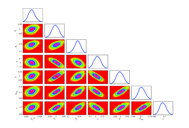
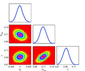
Figure 1: $1\sigma$ and $2\sigma$ contours of parameters for the VG-UM model with a CS fluid (left) and the $\Lambda$CDM (right) model.

	Mean values with limits (VG-UM)	Best fit (VG-UM)	Mean values with limits ($\Lambda$CDM)	Best fit ($\Lambda$CDM)
—-	$\Omega_{s}=-0.0106^{+0.0312+0.0582}_{-0.0305-0.0509}$	0.0006	$\Omega_{k}=-0.0002^{+0.0024+0.0052}_{-0.0024-0.0048}$	-0.0004
$\beta$	$-0.0128^{+0.0394+0.0756}_{-0.0385-0.0718}$	0.0005	0	0
$B_{s}$	$0.7457^{+0.0147+0.0269}_{-0.0145-0.0299}$	0.7520	—-	—-
$\alpha$	$0.0216^{+0.0757+0.1504}_{-0.0781-0.1466}$	0.0004	0	0
$h$	$0.6922^{+0.0149+0.0306}_{-0.0149-0.0289}$	0.6981	$0.6916^{+0.0100+0.0197}_{-0.0101-0.0193}$	0.6930
$100\Omega_{b}h^{2}$	$2.2580^{+0.0555+0.1154}_{-0.0557-0.1051}$	2.2691	$2.2683^{+0.0412+0.0815}_{-0.0420-0.0776}$	2.266
$\Omega_{0de}$	$0.6983^{+0.0165+0.0347}_{-0.0161-0.0309}$	0.7175	$0.7098^{+0.0144+0.0265}_{-0.0140-0.0294}$	0.7126

Table 4: The mean values with limits and the best-fit values of parameters for VG-UM model with a CS fluid.

In order to obtain the stringent constraint on VG theory, we utilize the cosmic data different from Ref. vg-field to calculate the joint likelihood. Concretely, the LT data, the GRBs data, the GF data, the SNIa data with systematic error and the BAO data from radial measurement are not used in Ref. vg-field . After calculation, the 1-dimension distribution and the 2-dimension contours of parameters for the VG-UM model with a CS fluid are illustrated in Fig. 1. From Fig. 1 and table 4, we can see that the restriction on dimensionless energy density of CS is $\Omega_{s}=-0.0106^{+0.0312+0.0582}_{-0.0305-0.0509}$ in the varying-$G$ theory with containing unified dark sectors. In the constant-$G$ theory, one knows that a CS fluid with $w_{s}=-1/3$ is usually equivalent to a curvature term. But, in the VG theory this equivalence is lost due to the term $a^{-\beta}$ multiplying the density, as shown in Eq.(4). Comparing the VG theory with the constant-$G$ theory, it can be seen that the uncertainty of $\Omega_{s}$ in VG theory is larger than some results on $\Omega_{k}$ in constant-$G$ theory. For example, using the same data to constrain other models we have $\Omega_{k}=-0.0002^{+0.0024+0.0052}_{-0.0024-0.0048}$ (with model parameter $\Omega_{0de}=0.7098^{+0.0144+0.0265}_{-0.0140-0.0294}$) in $\Lambda$CDM model, $\Omega_{k}=-0.0001^{+0.0025+0.0052}_{-0.0025-0.0050}$ (with model parameters $B_{s}=0.7665^{+0.0101+0.0194}_{-0.0099-0.0205}$ and $\alpha=0.0209^{+0.0186+0.0401}_{-0.0189-0.0373}$) in constant-$G$ UM. Taking the $\Lambda$CDM model as a reference, we can see that the influence on the fitting value of $\Omega_{k}$ is small from the added parameter $B_{s}$ and $\alpha$ as seen in constant-$G$ UM model, while the influence on the value of $\Omega_{s}$ is large by the added VG parameter $\beta$ as indicated in VG-UM model. From table 4, one reads VG parameter $\beta=-0.0128^{+0.0394+0.0756}_{-0.0385-0.0718}$. Other parameters are $B_{s}=0.7457^{+0.0147+0.0269}_{-0.0145-0.0299}$ and $\alpha=0.0216^{+0.0757+0.1504}_{-0.0781-0.1466}$. We then find at $1\sigma$ confidence level, the flat $\Lambda$CDM model ($\Omega_{s}=0$, $\beta=0$ and $\alpha=0$) is included in the VG-UM model with a CS fluid. This result in VG theory is same as the popular point that the complicated cosmological model is usually degenerate with the $\Lambda$CDM model.

IV.2 The case without a CS fluid

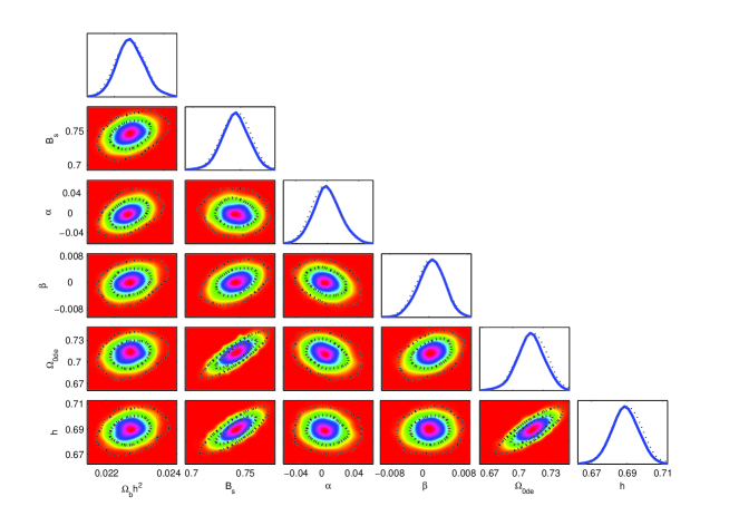
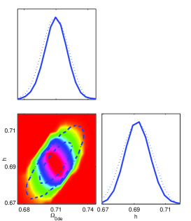
Figure 2: $1\sigma$ and $2\sigma$ contours of parameters for the VG-UM model without a CS fluid (left) and the $\Lambda$CDM (right) model.

	Mean values with limits (VG-UM)	Best fit (VG-UM)	Mean values with limits ($\Lambda$CDM)	Best fit ($\Lambda$CDM)
$\beta$	$0.0007^{+0.0032+0.0062}_{-0.0033-0.0067}$	0.0010	0	0
$B_{s}$	$0.7442^{+0.0137+0.0262}_{-0.0132-0.0292}$	0.7440	—-	—-
$\alpha$	$0.0002^{+0.0206+0.0441}_{-0.0209-0.0422}$	0.0073	0	0
$h$	$0.6905^{+0.0098+0.0191}_{-0.0096-0.0203}$	0.6902	$0.6925^{+0.0094+0.0207}_{-0.0104-0.0198}$	0.6923
$100\Omega_{b}h^{2}$	$2.267^{+0.054+0.116}_{-0.051-0.102}$	2.256	$2.2647^{+0.0398+0.0789}_{-0.0394-0.0781}$	2.262
$\Omega_{0de}$	$0.7093^{+0.0148+0.0296}_{-0.0150-0.0309}$	0.7095	$0.7101^{+0.0126+0.0270}_{-0.0135-0.0282}$	0.7106

Table 5: The mean values with limits and the best-fit values of model parameters for VG-UM model without a CS fluid.

For the case without a CS fluid, a stringent constraint on VG parameter is $\beta=0.0007^{+0.0032+0.0062}_{-0.0033-0.0067}$, where a small uncertainty at $2\sigma$ regions for $\beta$ is given. Still, it is shown that the value of $\beta$ is around zero at $1\sigma$ confidence level for both cases: including or not including a CS fluid, and the case containing a CS fluid has a larger error for $\beta$ than that not containing a CS fluid. In VG theory, the constraint on UM model parameters are $B_{s}=0.7442^{+0.0137+0.0262}_{-0.0132-0.0292}$, $\alpha=0.0002^{+0.0206+0.0441}_{-0.0209-0.0422}$, $h=0.6905^{+0.0098+0.0191}_{-0.0096-0.0203}$ and $100\Omega_{b}h^{2}=2.267^{+0.054+0.116}_{-0.051-0.102}$. At $1\sigma$ confidence level, the value of $\alpha=0$ is not excluded, which demonstrates that the $\Lambda$CDM model can not be distinguished from VG-UM model by the joint cosmic data. Besides the mean values with limits, the best-fit values of VG-UM model parameters are determined and exhibited in table 5, too. As a reference, the $\Lambda$CDM model is calculated by using the combined observational data appeared in section III, and the best-fit values and the mean values with limits on $\Lambda$CDM model are laid in table 5. In $\Lambda$CDM model, one receives $\Omega_{0de}=0.7101^{+0.0126+0.0270}_{-0.0135-0.0282}$ that is compatible to the effective result of $\Omega_{0de}$ in VG-UM model.

In order to agglomerate and form structure of universe, one knows that the baryonic (and DM) component must have a near zero pressure. Given that $w_{b}=\frac{p_{b}}{\rho_{b}}=\frac{-\beta(1-\beta)}{3(2+\beta)}\sim 0$, $\beta\sim 0$ or $\beta\sim 1$ could be solved. From above constraint on parameter $\beta$, one can see that the solution $\beta\sim 0$ is consistent with our fitting result for both cases: including or not including a CS fluid in universe.

V Behaviors of $G$ with the confidence level in VG-UM theory with or without a CS fluid

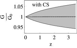
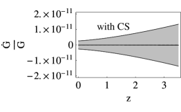
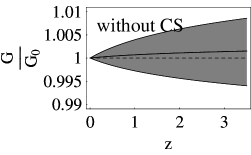
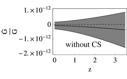
Figure 3: The best-fit evolutions of $\frac{{G}}{G_{0}}$ and $\frac{\dot{G}}{G}$ with their confidence level in VG-UM model containing (or not containing) a CS fluid.

	With CS	Without CS
$(\frac{G}{G_{0}})_{z=3.5}$	$1.0008^{+0.0620}_{-0.0584}$	$1.0015^{+0.0071}_{-0.0075}$
$(\frac{\dot{G}}{G})_{today}$	$-0.3496^{+26.3135}_{-26.3135}\times 10^{-13}yr^{-1}$	$-0.7252^{+2.3645}_{-2.3645}\times 10^{-13}yr^{-1}$
$(\frac{\dot{G}}{G})_{z=3.5}$	$-1.800^{+135.396}_{-135.396}\times 10^{-13}yr^{-1}$	$-3.792^{+12.314}_{-12.314}\times 10^{-13}yr^{-1}$

Table 6: The best-fit values of $\frac{G}{G_{0}}$ and $\frac{\dot{G}}{G}$ with their confidence level in VG-UM model containing (or not containing) a CS fluid.

Observations	Limits $(yr^{-1})$
Pulsating white dwarf G117-B15A VG-MNRAS-2004-dwarf	$\mid\frac{\dot{G}}{G}\mid\leq 4.1\times 10^{-10}$
Nonradial pulsations of white dwarfs VG-PRD-2004-white	$-2.5\times 10^{-10}\leq\frac{\dot{G}}{G}\leq 4\times 10^{-11}$
Millisecond pulsar PSR J0437-4715 VG-APJ	$\mid\frac{\dot{G}}{G}\mid\leq 2.3\times 10^{-11}$
Type-Ia Supernovae VG-PRD-2002-SN	$\frac{\dot{G}}{G}\leq 10^{-11}$
Neutron star masses VG-PRL-1996-neutron	$\frac{\dot{G}}{G}=(-0.6\pm 4.2)\times 10^{-12}$
Helioseismology VG-APJ-1998	$\mid\frac{\dot{G}}{G}\mid\leq 1.6\times 10^{-12}$
Lunar laser ranging experiment VG-PRL-2004-LL	$\frac{\dot{G}}{G}=(4\pm 9)\times 10^{-13}$
Big Bang Nuclei-synthesis VG-PRL-2004-BB	$-3.0\times 10^{-13}<\frac{\dot{G}}{G}<4.0\times 10^{-13}$

Table 7: Limits on the variation of $G$.

In VG-UM theory with or without a CS fluid, the best-fit evolutions of $\frac{\dot{G}}{G}$ with their confidence level (the shadow region) are illustrated in Figure 3 by using the best-fit values of model parameters with their covariance matrix. ”Dot” denotes the derivative with respect to $t$. In the VG-UM model with a CS fluid, limit on the variation of $G$ at today is $(\frac{\dot{G}}{G})_{today}\simeq-0.3496^{+26.3135}_{-26.3135}\times 10^{-13}yr^{-1}$, and at $z=3.5$ we have $(\frac{G}{G_{0}})_{z=3.5}\simeq 0.9917^{+0.0104}_{-0.0131}$ and $(\frac{\dot{G}}{G})_{z=3.5}\simeq-1.800^{+135.396}_{-135.396}\times 10^{-13}yr^{-1}$. For case without a CS fluid, Fig. 3 shows the prediction that the today’s value is $(\frac{\dot{G}}{G})_{today}\simeq-0.7252^{+2.3645}_{-2.3645}\times 10^{-13}yr^{-1}$. This restriction on $(\frac{\dot{G}}{G})_{today}$ is more stringent than other results seen in table 7. Also, using the best-fit value of parameter $\beta$ with error the shapes of $\frac{G}{G_{0}}=(1+z)^{\beta}$ are exhibited. Taking high redshift $z=3.5$ as another reference points, we find $(\frac{G}{G_{0}})_{z=3.5}\simeq 1.0015^{+0.0071}_{-0.0075}$ and $(\frac{\dot{G}}{G})_{z=3.5}\simeq-0.3792^{+1.2314}_{-1.2314}\times 10^{-12}yr^{-1}$ in the VG-UM model without a CS fluid. It is important to sternly constrain the value of $\beta$, since the monotonicity of $\frac{\dot{G}}{G}=-\beta H$ depends on the symbol of $\beta$. Fig. 3 reveal that the behaviors of $G$ and its derivative are around the constant-$G$ theory for both cases: including or not including a CS fluid in universe.

VI Behaviors of EoS with the confidence level in VG-UM theory with or without a CS fluid

The EoS of UM in VG theory is demonstrated

$$w_{VG-UM}(z)=\frac{p_{VG-UM}}{\rho_{VG-UM}}=\frac{\beta-3}{3}\frac{B_{s}}{B_{s}+(1-B_{s})(1+z)^{(1+\alpha)(3-\beta)}}.$$ (49)

From Figure 4 (left), we can see that $w_{VG-UM}\sim 0$ (DM) at early time and $w_{VG-UM}\sim-1$ (DE) in the future for the VG-UM model with or without a CS fluid. If the dark sectors are thought to be separable, it is interested to investigate the properties of both dark components in VG-UM model. Supposing that the behavior of dark matter is known i.e. its EoS $w_{dm}=0$ ($\rho_{dm}=\rho_{0dm}a^{\frac{-\beta^{2}-2\beta-6}{2+\beta}}$), the EoS of dark energy in VG-UM model subjects to

$$w_{de}=\frac{p_{de}}{\rho_{de}}=\frac{p_{VG-UM}}{\rho_{VG-UM}-\rho_{dm}}=\frac{-A}{\rho_{VG-UM}^{1+\alpha}-\rho_{dm}\rho_{VG-UM}^{\alpha}}.$$ (50)

Using the best-fit values of model parameters and the covariance matrix, the evolutions of $w_{de}$ with confidence level in VG-UM model containing (or not containing) a CS fluid are plotted in Fig. 4 (middle). If one deems the behavior of dark energy is the cosmological constant i.e. $w_{\Lambda}=-1$ ($p_{\Lambda}=-\rho_{\Lambda}$), the EoS of dark matter in VG-UM model obeys

$$w_{dm}=\frac{p_{dm}}{\rho_{dm}}=\frac{p_{VG-UM}-p_{\Lambda}}{\rho_{VG-UM}-\rho_{\Lambda}}=\frac{\rho_{\Lambda}\rho_{VG-UM}^{\alpha}-A}{\rho_{VG-UM}^{1+\alpha}-\rho_{\Lambda}\rho_{VG-UM}^{\alpha}}$$ (51)

which is drawn in Fig. 4 (right) with the confidence level for two cases (with or without a CS fluid).

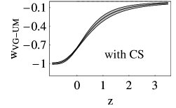
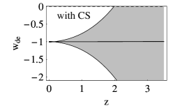
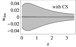
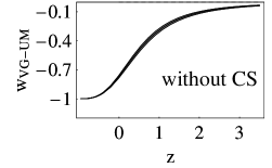
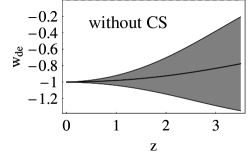
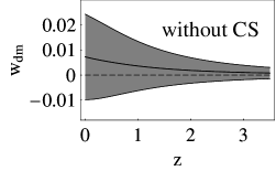
Figure 4: The evolutions of EoS with confidence level in VG-UM model including (lower) or not including (upper) a CS fluid. Evolution of $w_{VG-UM}(z)$ (left), evolution of $w_{de}(z)$ in VG-UM model with assuming $w_{dm}=0$ at prior (middle), and evolution of $w_{dm}(z)$ in VG-UM model with assuming $w_{de}=-1$ at prior (right).

	$w_{0VG-UM}$	$w_{0dm}$ (with $w_{0de}=-1$)	$w_{0de}$ (with $w_{0dm}=0$)
With CS	$-0.7519^{+0.0112}_{-0.0112}$	$0.0009^{+0.0304}_{-0.0304}$	$-0.9998^{+0.0125}_{-0.0125}$
Without CS	$-0.7438^{+0.0134}_{-0.0134}$	$0.0072^{+0.0170}_{-0.0170}$	$-0.9986^{+0.0011}_{-0.0011}$

Table 8: The best-fit values of $w_{0VG-UM}$, $w_{0dm}$ and $w_{0de}$ with their confidence level hinted by VG-UM model with or without a CS fluid.

From Fig. 4, we get the current values $w_{0dm}=0.0009^{+0.0304}_{-0.0304}$ in VG-UM model with a CS fluid and $w_{0dm}=0.0072^{+0.0170}_{-0.0170}$ in VG-UM model without a CS fluid, which have the larger uncertainties than $w_{0dm}=0.0010^{+0.0016}_{-0.0016}$ calculated on the non-unified model of constant-$G$ theory by Ref. wdm . For the current value $w_{0de}$, it approximates to -1 with the very small uncertainty for both VG-UM model with a CS fluid ($w_{0de}=-0.9998^{+0.0125}_{-0.0125}$) and VG-UM model without a CS fluid ($w_{0de}=-0.9986^{+0.0011}_{-0.0011}$). From the best fit evolution in VG-UM model with a CS fluid, we can see that both $w_{de}(\sim-1)$ and $w_{dm}(\sim 0)$ tends to be constant, but the uncertainties of them are much larger than that in model without a CS fluid. For the best-fit evolution in VG-UM model without a CS fluid, $w_{de}$ and $w_{dm}$ are variable with the time and $w_{dm}$ tends to have small deviation from zero (small-positive pressure) at the recent time. In addition, at high redshift the uncertainty of $w_{de}$ (or $w_{dm}$) is enlarged (or narrowed) for both VG-UM model with a CS fluid and VG-UM model without a CS fluid.

VII Perturbational behaviors in structure formation for VG-UM theory

The study on the structure formation is necessary for a cosmological theory. We investigate the evolutions of growth function $f$ and growth factor $D$ in VG-UM theory. The derivation of evolutionary equation $f$ and $D$ are shown in appendix. Using the definition $f(a)=\frac{aD^{{}^{\prime}}(a)}{D(a)}=\frac{d\ln\delta}{d\ln a}$, we obtain the dynamically evolutionary equation of $f$

$$(1+z)f^{\prime}-f^{2}+(1+z)f\frac{E^{\prime}}{E}-\frac{4+2\beta+2\beta^{2}}{2+\beta}f+\frac{6+2\beta+\beta^{2}}{(2+\beta)^{2}}\frac{\Omega_{0m}}{E^{2}}(1+z)^{\frac{6+2\beta+\beta^{2}}{2+\beta}}=0$$ (52)

where prime denotes the derivative with respect to redshift $z$ and $E(z)=H(z)/H_{0}$.

Figure 5: The evolutions of $f(z)$, $f(a)$ and $D(a)$. The solid lines correspond to the $\Lambda$CDM model, the short-dash lines correspond to the VG-UM model with a CS fluid, and the dot lines correspond to the VG-UM model without a CS fluid.

In Fig. 5, we use the best-fit values of cosmological parameters in table 4 and 5 to plot the evolutions of growth function $f$ and growth factor $D$ for VG-UM model and $\Lambda$CDM model by numerically solving Eq. (24) and (52) with the initial conditions $a_{i}=0.0001$, $D(a_{i})=a_{i}$, $D^{{}^{\prime}}(a_{i})=0$ and $f(a_{i})=1$. We can see that the evolutions of $f(a)$ for VG-UM model (including or not including a CS fluid) fit well as $\Lambda$CDM model, and the behavior of $f(z)$ are well consistent with the observational growth data listed in table 3. In VG-UM model with or without a CS fluid, $D(a)$ evolves slower (more slow growth of perturbations) than that in the $\Lambda$CDM model. The current value of $D(a=1)$ in $\Lambda$CDM model is approximately 12% larger than that in VG-UM model without a CS fluid.

VIII Conclusions

Observations anticipate that $G$ may be variable and most universal energy density are invisible. The attractive properties of this study is that the variation of $G$ naturally results to the invisible components in universe. The VG could provide a solution to the originated problem of DM and DE. We apply recently observed data to constrain the unified model of dark sectors with or without a CS fluid in the framework of VG theory. Using the LT, the GRBs, the GF, the SNIa with systematic error, the CMB from 9-year WMAP and the BAO data from measurement of radial and peak positions, uncertainties of VG-UM parameter space are obtained.

For the case without a cosmic string fluid, constraint on mean value of VG parameter is $\beta=0.0007^{+0.0032+0.0062}_{-0.0033-0.0067}$ with a small uncertainty around zero, and restrictions on UM model parameters are $B_{s}=0.7442^{+0.0137+0.0262}_{-0.0132-0.0292}$ and $\alpha=0.0002^{+0.0206+0.0441}_{-0.0209-0.0422}$ with $1\sigma$ and $2\sigma$ confidence level. For the case with a cosmic string fluid, restriction on dimensionless density parameter of CS fluid is $\Omega_{s}=-0.0106^{+0.0312+0.0582}_{-0.0305-0.0509}$ in the VG-UM theory. Obviously, the uncertainty of $\Omega_{s}$ is larger than some results on $\Omega_{k}$ in the framework of $G$-constant theory. At $1\sigma$ confidence level the flat $\Lambda$CDM model ($\Omega_{s}=0$, $\beta=0$ and $\alpha=0$) is included in the VG-UM model.

Using the best-fit values of VG-UM parameters and their covariance matrix, the limits on today’s value are $(\frac{\dot{G}}{G})_{today}=-0.7252^{+2.3645}_{-2.3645}\times 10^{-13}$ or $(\frac{\dot{G}}{G})_{today}\simeq-0.3496^{+26.3135}_{-26.3135}\times 10^{-13}yr^{-1}$ for the universe with or without a CS fluid. And corresponding to these two cases, we finds $(\frac{G}{G_{0}})_{z=3.5}\simeq 1.0015^{+0.0071}_{-0.0075}$ and $(\frac{G}{G_{0}})_{z=3.5}\simeq 1.0008^{+0.0620}_{-0.0584}$ at redshift $z=3.5$. If one considers that the DM and the DE could be separable in unified model, EoS of DE and DM are discussed by combing with the fitting results. It is shown that $w_{0dm}=0.0072^{+0.0170}_{-0.0170}$ or $w_{0dm}=0.0009^{+0.0304}_{-0.0304}$ with assuming $w_{0de}=-1$ for VG-UM universe containing or not containing a CS fluid, while there are $w_{0de}=-0.9986^{+0.0011}_{-0.0011}$ or $w_{0de}=-0.9998^{+0.0125}_{-0.0125}$ with assuming $w_{0dm}=0$ at prior for VG-UM model with or without a CS fluid.

Acknowledgments The research work is supported by the National Natural Science Foundation of China (11205078,11275035,11175077).

Appendix A The growth of structures in linear perturbation theory

In a sub-horizon region with length scale $r<H^{-1}$, the density of DE and cold DM are expressed by $\tilde{\rho}_{sde}$ and $\tilde{\rho}_{sdm}$, respectively. We suppose that DE is not perturbed, DM is perturbed in sub-horizon region. So, we have $\tilde{\rho}_{sde}=\rho_{de}$ for the homogeneous DE in whole universe and $\tilde{\rho}_{sdm}=\rho_{dm}+\delta\rho_{dm}$ for the perturbed DM, where $\rho_{de}$ and $\rho_{dm}$ denote the density of DE and DM in background level, respectively. Obviously, the region of $\delta\rho_{dm}>0$ will cluster and form structure. In analogy to the equation in background level, the evolution of matter density inside the perturbed region can be given by the following conservation equation

$$\dot{\tilde{\rho}}_{sdm}+3h(\frac{6+2\beta+\beta^{2}}{6+3\beta}\tilde{\rho}_{sdm}+\frac{2+2\beta}{2+\beta}\tilde{p}_{sdm})=0.$$ (53)

Symbol ”tilde” denotes the cosmological quantity in perturbed region. In this region, the local expansion is described by $h=\dot{r}/r$ and the acceleration is

$$\frac{\ddot{r}}{r}=-\frac{8\pi G(t)}{3(2+\beta)}(\tilde{\rho}_{sdm}+\rho_{de}+3\tilde{p}_{sdm}+3p_{de})-\frac{\beta^{2}}{(2+\beta)}h$$ (54)

which is same as Eq.(5) for background level. One can define the density contrast of DM

$$1+\delta_{dm}=\frac{\tilde{\rho}_{sdm}}{\rho_{dm}}$$ (55)

with $\delta_{dm}>0$. Differentiating Eq. (55) with respect to $t$ gives

$$\dot{\delta}_{dm}+(\frac{6+2\beta+\beta^{2}}{2+\beta})(1+\delta_{dm})(h-H)+\frac{6+6\beta}{2+\beta}(1+\delta_{dm})(h\tilde{w}_{sdm}-Hw_{dm})=0$$ (56)

after using Eqs. (53) and (6). Taking the time derivative in above equation obtains

$$\ddot{\delta}_{dm}-\frac{\dot{\delta}_{dm}^{2}}{1+\delta_{dm}}+(\frac{6+2\beta+\beta^{2}}{2+\beta})(1+\delta_{dm})(\dot{h}-\dot{H})+\frac{6+6\beta}{2+\beta}(\dot{h}\tilde{w}_{sdm}+h\dot{\tilde{w}}_{sdm}-\dot{H}\tilde{w}_{sdm}-H\dot{\tilde{w}}_{sdm})(1+\delta_{dm})=0,$$ (57)

where

$$\dot{h}-\dot{H}=-\frac{H^{2}}{2+\beta}\Omega_{dm}\delta_{dm}-\frac{4+2\beta+2\beta^{2}}{2+\beta}(h-H)H-\frac{3H^{2}}{2+\beta}(\frac{\tilde{\rho}_{sdm}}{\tilde{\rho}_{c}}\tilde{w}_{sdm}-\Omega_{dm}w_{dm})$$ (58)

is given by substituting Eqs. (5) and (54) into $\dot{H}=\frac{\ddot{a}}{a}-H^{2}$ and $\dot{h}=\frac{\ddot{r}}{r}-h^{2}$, respectively. In addition, in calculation we used $\rho_{c}=3H^{2}/8\pi G(t)$ and $h+H\simeq 2H$. Inserting (58) into (57) results

$$\ddot{\delta}_{dm}-\frac{\dot{\delta}_{dm}^{2}}{1+\delta_{dm}}+\frac{4+2\beta+\beta^{2}}{2+\beta}H\dot{\delta}_{dm}-(\frac{6+2\beta+\beta^{2}}{2+\beta})\frac{H^{2}\Omega_{dm}}{2+\beta}(\delta_{dm}+\delta_{dm}^{2})$$

$$+[\frac{4+2\beta+2\beta^{2}}{2+\beta}\frac{6+6\beta}{2+\beta}H(h\tilde{w}_{sdm}-Hw_{dm})+\frac{6+6\beta}{2+\beta}(\dot{h}w_{dm}+h\dot{\tilde{w}}_{sdm}-\dot{H}w_{dm}-H\dot{w}_{dm})$$

$$+(\frac{6+2\beta+\beta^{2}}{2+\beta})\frac{3H^{2}}{2+\beta}(\frac{\tilde{\rho}_{sdm}}{\tilde{\rho}_{c}}\tilde{w}_{sdm}-\Omega_{dm}w_{dm})](1+\delta_{dm})=0.$$ (59)

Neglecting square terms of $\delta_{m}$ in (59), we receive the evolutional equation of density contrast in spherical overdense region

$$\ddot{\delta}_{dm}+\frac{4+2\beta+2\beta^{2}}{2+\beta}H\dot{\delta}_{dm}-(\frac{6+2\beta+\beta^{2}}{2+\beta})\frac{H^{2}\Omega_{dm}}{2+\beta}\delta_{dm}+[\frac{4+2\beta+2\beta^{2}}{2+\beta}\frac{6+6\beta}{2+\beta}H(h\tilde{w}_{sdm}-Hw_{dm})$$

$$+\frac{6+6\beta}{2+\beta}(\dot{h}\tilde{w}_{sdm}+h\dot{w}_{dm}-\dot{H}\tilde{w}_{sdm}-H\dot{w}_{sdm})+(\frac{6+2\beta+\beta^{2}}{2+\beta})\frac{3H^{2}}{2+\beta}(\frac{\tilde{\rho}_{sdm}}{\tilde{\rho}_{c}}\tilde{w}_{sdm}-\Omega_{dm}w_{dm})](1+\delta_{dm})=0.$$ (60)

Taking $\beta=0$, the above equation reduces to case of constant $G$ given by reference D-G . Using the definition of growth factor $D(a)$, we can rewrite Eq. (60) as follows

$$D^{{}^{\prime\prime}}(a)+[\frac{E^{{}^{\prime}}(a)}{E(a)}+\frac{1}{a}+\frac{4+2\beta+2\beta^{2}}{a(2+\beta)}]D^{{}^{\prime}}(a)-\frac{6+2\beta+\beta^{2}}{(2+\beta)^{2}}\frac{\Omega_{0dm}}{E(a)^{2}a^{2}}a^{\frac{-6-2\beta-\beta^{2}}{2+\beta}}D(a)$$

$$+[\frac{(4+2\beta+2\beta^{2})(6+6\beta)}{(2+\beta)^{2}a^{2}H}(h\tilde{w}_{sdm}-Hw_{dm})+\frac{6+6\beta}{(2+\beta)aH}(h^{{}^{\prime}}\tilde{w}_{sdm}+h\tilde{w}^{{}^{\prime}}_{sdm}-H^{{}^{\prime}}w_{dm}-Hw^{{}^{\prime}}_{dm})$$

$$+\frac{18+6\beta+3\beta^{2}}{(2+\beta)^{2}a^{2}}(\frac{\tilde{\rho}_{sdm}}{\tilde{\rho}_{c}}\tilde{w}_{sdm}-\Omega_{dm}w_{dm})][1+D(a)\delta_{dm}(a=1)]=0.$$ (61)

The linear regime of cosmological perturbations is valid for all sales during the early radiation dominated era and for most sales during the matter dominated era. For $w_{dm}\simeq w_{sdm}\simeq 0$, above equation reduces to

$$D^{{}^{\prime\prime}}(a)+[\frac{E^{{}^{\prime}}(a)}{E(a)}+\frac{1}{a}+\frac{4+2\beta+2\beta^{2}}{a(2+\beta)}]D^{{}^{\prime}}(a)-\frac{6+2\beta+\beta^{2}}{(2+\beta)^{2}}\frac{\Omega_{0dm}}{E(a)^{2}a^{2}}a^{\frac{-6-2\beta-\beta^{2}}{2+\beta}}D(a)=0.$$ (62)

Transferring the function from $D$ to $f$ in above equation, we get

$$f^{{}^{\prime}}(a)+\frac{f^{2}(a)}{a}+[\frac{E^{{}^{\prime}}(a)}{E(a)}+\frac{2}{a}(\frac{2+\beta+\beta^{2}}{(2+\beta)})]f(a)-\frac{6+2\beta+\beta^{2}}{(2+\beta)^{2}}\frac{\Omega_{0dm}}{E(a)^{2}a}a^{\frac{-6-2\beta-\beta^{2}}{2+\beta}}=0.$$ (63)

References

- (1) K.I. Umezu, K. Ichiki and M. Yahiro, Physical Review D 72, 044010 (2005).
- (2) M. Biesiada and B. Malec, Mon. Not. Roy. Astron. Soc. 350, 644 (2004) [astro-ph/0303489].
- (3) O. G. Benvenuto et al., Phys. Rev. D, 69, 082002, (2004).
- (4) J.P.W. Verbiest et al., Astrophys. J. 679, 675 (2008) [arXiv:0801.2589].
- (5) E. Gaztanaga, et al, Phys. Rev. D 65, 023506, 2002 [arXiv:astro-ph/0109299].
- (6) S. E. Thorsett, Phys. Rev. Lett. 77, 1432 (1996) [astro-ph/9607003].
- (7) L.X. Xu, J.B. Lu, Y.T. Wang, Eur. Phys. J. C 72 1883 (2012), [arXiv:1204.4798].
- (8) P.X. Wu and H.W. Yu, Phys. Lett. B, 644, 16 (2007).
- (9) K. Zhang, P.X. Wu and H.W. Yu,JCAP 01 (2014) 048.
- (10) A. Ali, S. Dutta, E. N. Saridakis, A. A. Sen [arXiv:1004.2474].
- (11) C. Ranjit, P. Rudra, S. Kundu, [arXiv:1304.6713].
- (12) S. Ghose, A. Saha, B.C. Paul, [arXiv:1203.2113].
- (13) S. Mukherjee, B. C. Paul, N. K. Dadhich, S. D. Maharaj, A. Beesham, Class.Quant.Grav. 23 (2006) 6927
- (14) S. Ghose, P. Thakur, B. C. Paul, Mon. Not. R. Astron. Soc. 421, 20 (2012) [arXiv:1105.3303]
- (15) T. Harko, M. J. Lake, [arXiv:1409.8454]
- (16) F. Niedermann, R. Schneider, Phys.Rev. D91, 064010 (2015) , [arXiv:1412.2750]
- (17) S. Kumar, A. Nautiyal, A. A. Sen, [arXiv:1207.4024]
- (18) O. S. Sazhina, D. Scognamiglio, M. V. Sazhin, [arXiv:1312.6106]
- (19) M. van de Meent, Phys. Rev. D 87, 025020 (2013), [arXiv:1211.4365]
- (20) P. A. R. Ade, et al, [arXiv:1303.5085]
- (21) A. Lewis and S. Bridle, Phys. Rev. D, 66, 103511 (2002).
- (22) S. Capozziello, V. F. Cardone, M. Funaro, and S. Andreon, Phys. Rev. D 70, 123501 (2004).
- (23) Simon, J., Verde, L., Jimenez, R. 2005, Phys. Rev. D, 71, 123001.
- (24) L. Xu, JCAP 04 (2012) 025 [arXiv:1005.5055].
- (25) L. Verde et al., Mon. Not. Roy. Astron. Soc. 335, 432 (2002) [astro-ph/0112161].
- (26) E. V. Linder, Astropart. Phys., 29, 336-339, (2008) [arXiv:0709.1113].
- (27) C. Blake et al., Mon. Not. Roy. Astron. Soc. 415, 2876 (2011) [arXiv:1104.2948].
- (28) R. Reyes et al., Nature. 464, 256, (2010) [arXiv:1003.2185].
- (29) M. Tegmark et al. [SDSS Collaboration], Phys. Rev. D 74, 123507 (2006) [astro-ph/0608632].
- (30) N.P. Ross et al., Mon. Not. Roy. Astron. Soc., 381, Issue 2, 573-588, (2007) [astro-ph/0612400].
- (31) L. Guzzo et al., Nature 451, 541 (2008) [arXiv:0802.1944].
- (32) J. da Angela et al., Mon. Not. Roy. Astron. Soc., 383, Issue 2, 565-580, (2008) [astro-ph/0612401].
- (33) R. Amanullah et al. [Supernova Cosmology Project Collaboration], [arXiv:1004.1711].
- (34) G. Hinshaw et al., [arXiv:astro-ph/1212.5226].
- (35) E. Gaztanaga, R. Miquel, E. Sanchez, Phys. Rev. Lett. 103 091302(2009).
- (36) C. Blake et al, [arXiv:1108.2635].
- (37) Beutler F., et al., [arXiv:1106.3366].
- (38) W.J. Percival et al., Mon. Not. R. Astron. Soc. 401, 2148 (2010), [arXiv:astro-ph/0907.1660].
- (39) J.B. Lu, L.X. Xu, H.Y. Tan, and S.S. Gao, Phys. Rev. D 89, 063526 (2014).
- (40) M.C. Bento, O. Bertolami and A.A. Sen, Phys. Rev. D 66 (2002) 043507.
- (41) A. Sandage, Annu. Rev. Astron. Astrophys. 26, 561 (1988).
- (42) N. Pires, Z. Zhu, J. S. Alcaniz, Phys.Rev.D 73, 123530 (2006).
- (43) M. A. Dantas, J. S. Alcaniz, D. Jain, A.Dev, Astron. Astrophys. 467 (2007) 421.
- (44) E. Komatsu et al. [WMAP Collaboration], [arXiv:1001.4538].
- (45) B. E. Schaefer, Astrophys. J. 660, 16 (2007) [astro-ph/0612285].
- (46) L. Amati et al., Mon. Not. Roy. Astron. Soc. 391, 577 (2008) [arXiv:0805.0377].
- (47) Y. Wang, Phys.Rev.D 78,123532(2008).
- (48) M. C. Bento, O. Bertolami and A. A. Sen 2003 Phys. Lett. B 575 172.
- (49) M. Li, X. D. Li and X. Zhang, 2010 Sci. China. Ser. G 53 1631.
- (50) P.T. Silva and O. Bertolami, 2003 Astrophys. J. 599 829.
- (51) A.C.C. Guimaraes, J.V. Cunha and J.A.S. Lima, JCAP, 0910, 010 (2009).
- (52) M. Szydlowski and W. Godlowski, Phys. Lett. B, 633, 427 (2006).
- (53) R.G. Cai, Q. Su, H.B. Zhang, Accepted by JCAP, [arXiv:astro-ph/1001.2207].
- (54) R.G. Cai, Q. P. Su, Phys.Rev.D81:103514,2010.
- (55) Y.G. Gong, R.G. Cai, Y. Chen, Z.H. Zhu, JCAP 01 (2010) 019.
- (56) Y.G. Gong, B. Wang, R.G. Cai, JCAP 04 (2010) 019.
- (57) R.Gannouji, D. Polarski, JCAP 0805, 018 (2008).
- (58) J.B. Lu, L.X. Xu, and M.L. Liu, Phys. Lett. B 699 (2011) 246-250.
- (59) Z.X. Li, P.X. Wu, H.W. Yu, et al, SCIENCE CHINA Physics, Mechanics Astronomy 57 (2014) 381.
- (60) J.F. Zhang, L. Zhao, X. Zhang, SCIENCE CHINA Physics, Mechanics Astronomy 57 (2014) 387.
- (61) S. Nesseris and L. Perivolaropoulos, Phys. Rev. D 72 123519 (2005).
- (62) L. Perivolaropoulos, Phys. Rev. D 71 063503 (2005).
- (63) E. Di Pietro and J. F. Claeskens, Mon. Not. Roy. Astron. Soc. 341 1299 (2003).
- (64) C. Cheng, Q.G. Huang, SCIENCE CHINA Physics, Mechanics Astronomy 58 (2015) 099801.
- (65) J.B. Lu, et al, SCIENCE CHINA Physics, Mechanics Astronomy 57 (2014) 796.
- (66) V. Acquaviva and L. Verde, JCAP 0712 001 (2007).
- (67) E. Garcia-Berro, E. Gaztanaga, J. Isern, O. Benvenuto and L. Althaus, astro-ph/9907440.
- (68) A. Riazuelo and J. Uzan, Phys. Rev. D 66 023525 (2002).
- (69) L.X. Xu, Phys. Rev. D 91, 063008 (2015).
- (70) L.X. Xu, JCAP 02 (2014) 048.
- (71) http://supernova.lbl.gov/Union/
- (72) J.B. Lu, D.H. Geng, L.X. Xu, Y.B. Wu and M.L. Liu, JHEP 02, 071 (2015).
- (73) Z.X. Li, P.X. Wu, H.W. Yu and Z.H. Zhu, Physical Review D 87, 103013 (2013).
- (74) S. Nesseris, J. Garcia-Bellido, JCAP11(2012)033, [arXiv:astro-ph/1205.0364].
- (75) D. B. Guenther, L. M. Krauss, and P. Demarque, Astrophys. J. 498, 871 (1998).
- (76) J. G. Williams, S. G. Turyshev and D. H. Boggs, Phys. Rev. Lett. 93, 261101 (2004) [gr-qc/0411113].
- (77) C. J. Copi, A. N. Davies, L. M. Krauss, Phys. Rev. Lett., 92, 171301, (2004).
- (78) L.X. Xu, Y.D. Chang, Phys. Rev. D 88, 127301 (2013) [arXiv:1310.1532].
- (79) T. Padmanabhan, Structure formation in the universe ,Cambridge University Press, (1993).