Distributed execution of bigraphical reactive systems

Abstract

The bigraph embedding problem is crucial for many results and tools about bigraphs and bigraphical reactive systems (BRS). Current algorithms for computing bigraphical embeddings are centralized, i.e. designed to run locally with a complete view of the guest and host bigraphs. In order to deal with large bigraphs, and to parallelize reactions, we present a decentralized algorithm, which distributes both state and computation over several concurrent processes. This allows for distributed, parallel simulations where non-interfering reactions can be carried out concurrently; nevertheless, even in the worst case the complexity of this distributed algorithm is no worse than that of a centralized algorithm.

1 Introduction

Bigraphical Reactive Systems (BRSs) [10, 16] are a flexible and expressive meta-model for ubiquitous computation. In the last decade, BRSs have been successfully applied to the formalization of a wide range of domain-specific calculi and models, from traditional programming languages to process calculi for concurrency and mobility, from business processes to systems biology; a non exhaustive list is [3, 4, 1, 6, 14, 12]. Recently, BRSs have found a promising applications in structure-aware agent-based computing: the knowledge about the (physical) world where the agents operate (e.g., drones, robots, etc.) can be conveniently represented by means of BRSs [17, 22]. BRSs are appealing also because they provide a range of general results and tools, which can be readily instantiated with the specific model under scrutiny: simulation tools, systematic construction of compositional bisimulations [10], graphical editors [7], general model checkers [20], modular composition [19], stochastic extensions [11], etc.

This expressive power stems from the rich structure of bigraphs, which are the states of a bigraphic reactive system. A bigraph is a compositional data structure describing at once both the locations and the connections of (possibly nested) system components. To this end, bigraphs combine two independent graphical structures over the same set of nodes: a hierarchy of places, and a hypergraph of links. Intuitively, places represent (physical) positions of agents, while links represent logical connections between agents. A simple example is shown in Figure 1.

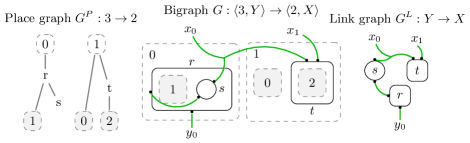
Figure 1: Forming a bigraph from a place graph and a link graph.

The behaviour of a BRS is defined by a set of (parametric) reaction rules, like in graph rewriting [21]. Applying a reaction rule to a bigraph corresponds to find an embedding of the rule’s redex and replace it with the corresponding reactum. Thus, BRSs can be run (or simulated) by the abstract machine depicted in Figure 2 (or variants of it). This machine is composed by two main modules: the embedding engine and the reaction engine. The former keeps track of available redex embeddings into the bigraph in the current machine state; the latter is responsible of carrying out the reactions, in two steps: (a) choosing an occurrence of a redex among those provided by the embedding engine and (b) updating the machine state by performing the chosen rewrite operation.

The choice of which reaction to perform is driven by user-provided execution policies. A possible simple policy is the random selection of any available reactions, while in [12] execution policies are based on agent believes, intentions and goals. Execution policies are outside the scope of this paper, and we refer the reader to [18] for other examples. Here we mention LibBig, an extensible library for bigraphical reactive systems (available at http://mads.dimi.uniud.it/) which offers easily customizable execution policies in the form of cost-based embeddings where costs are defined at the component level via attached properties.

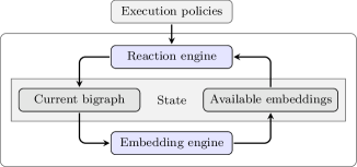
Figure 2: The open cycle of an abstract bigraphical machine.

Therefore, computing bigraph embeddings (i.e., finding the occurrences of a bigraph, called guest, inside another one, called host) is a central issue in any implementation of a BRS abstract machine. The problem is known to be NP-complete [2], and some algorithms (or reductions) can be found in the literature [8, 15, 23]. However, existing algorithms assume a complete view of both the guest and the host bigraphs. This hinders the scalability of BRS execution tools, especially on devices with low resources (like embedded ones). Moreover, in a truly distributed setting (like in multi-agent systems [12]) the bigraph is scattered among many machines; gathering it to a single “knowledge manager” in order to calculate embeddings and apply the rewriting rules, would be impractical.

In this paper, we aim to overcome these problems, by introducing an algorithm for computing bigraphical embeddings in distributed settings where bigraphs are spread across several cooperating processes. This decentralized algorithm does not require a complete view of the host bigraph, but retains the fundamental property of (eventually) computing every possible embedding for the given host. Thanks to the distributed nature of the algorithm, this solution can scale to bigraphs that cannot fit into the memory of a single process, hence too large to be handled by existing implementations. Moreover, the algorithm is parallelized: several (non-interfering) reductions can be identified and applied at once. In this paper we consider distributed host bigraphs only since guest bigraphs are usually redexes of parametric reaction rules and hence small enough to be handled even in presence of scarce computational resources.

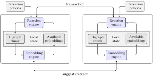
Figure 3: D-BAM: Distributed bigraphical abstract machine.

This algorithm is the core of a decentralized version of the abstract bigraphical machine illustrated above. The architecture of this new distributed bigraphical (abstract) machine (D-BAM) is in Figure 3. Both computation and states are distributed over a family of processes. Each process has only a partial view of the global state and negotiates updates to its piece of the global bigraph with its “neighbouring processes”. We assume reliable asynchronous point-to-point communication between reliable processes; this is a mild assumptions for a distributed system and can be easily achieved e.g. over unreliable channels.

This work extends and improves [13] in several ways. First, we introduce a new compact representation of partial embeddings, reducing both network and memory footprint of the distributed embedding algorithm; secondly, messages are routed across the overlay network only to processes that can benefit from their content (in [13] messages were forwarded to the entire neighbourhood). Moreover, we discuss some other heuristics and partition strategies.

Synopsis

In Section 2 we briefly recall bigraphical reactive systems and bigraph embeddings. In Section 3 we introduce the notion of partial bigraph embedding and the weaker notion of candidate partial bigraph embedding. In Section 4 and Section 5 we describe the D-BAM; in particular we show how to solve the embedding problem at its core by means of a distributed algorithm which incrementally computes (candidate) partial bigraph embeddings. Conclusions and final remarks are discussed in Section 6.

2 Bigraphs and their embeddings

In this section we briefly recall the notion of bigraphs, Bigraphical Reactive Systems (BRS), and bigraph embedding; for more detail we refer to [16].

2.1 Bigraphical reactive systems

The idea at the core of BRSs is that agents may interact in a reconfigurable space, even if they are spatially separated. This means that two agents may be adjacent in two ways: they may be at the same place, or they may be connected by a link. Hence, the state of the system is represented by a bigraph, i.e., a data structure combining two independent graphical structures over the same set of nodes: a hierarchy of places, and a hyper-graph of links

Definition 1 (Bigraph [16, Def. 2.3]).

Let $\Sigma$ be a bigraphical signature (i.e. a set of controls, each associated with a finite arity). A bigraph $G$ over $\Sigma$ is an object

$$(V_{G},E_{G},\textsf{{ctrl}}_{G},\textsf{{prnt}}_{G},\textsf{{link}}_{G}):\langle n_{G},X_{G}\rangle\to\langle m_{G},Y_{G}\rangle$$

composed of two substructures (cf. Figure 1): a place graph $G^{P}=(V_{G},\textsf{{ctrl}}_{G},\textsf{{prnt}}_{G}):{n_{G}\to m_{G}}$ and a link graph $G^{L}=(V_{G},E_{G},\textsf{{ctrl}}_{G},\textsf{{link}}_{G}):{X_{G}\to Y_{G}}$. The set $V_{G}$ is a finite set of nodes and to each of them is assigned a control in $\Sigma$ by the control map $\textsf{{ctrl}}_{G}:V_{G}\to\Sigma$. The set $E_{G}$ is a finite set of names called edges. These structures present an inner interface (composed by $m_{G}$ and $X_{G}$) and an outer one ($n_{G}$, $Y_{G}$) along which can be composed with other of their kind as long as they do not share any node or edge. In particular, $X_{G}$ and $Y_{G}$ are finite sets of names and $m_{G}$ and $n_{G}$ are finite ordinals (that index sites and roots respectively). On the side of $G^{P}$, nodes, sites and roots are organized in a forest described by the parent map $\textsf{{prnt}}_{G}:V_{G}\uplus m_{G}\to V_{G}\uplus n_{G}$. On the side of $G^{L}$, nodes, edges and names of the inner and outer interface forms a hyper-graph described by the link map $\textsf{{link}}_{G}:P_{G}\uplus X_{G}\to E_{G}\uplus Y_{G}$ which is a function from $X_{G}$ and ports $P_{G}$ (i.e. elements of the finite ordinal associated to each node by its control) to edges $E_{G}$ and outer names $Y_{G}$.

The dynamic behaviour of a system is described in terms of reactions of the form $a\rightarrowtriangle a^{\prime}$ where $a,a^{\prime}$ are agents, i.e. bigraphs with inner interface $\langle 0,\emptyset\rangle$. Reactions are defined by means of graph rewrite rules, which are pairs of bigraphs $(R_{L},R_{R})$ equipped with a function $\eta$ from the sites of $R_{R}$ to those of $R_{L}$ called instantiation rule. A bigraphical encoding for the open reaction rule of the Ambient Calculus is shown in Figure 4 where redex and reactum are the bigraph on the left and the one on the right respectively and the instantiation rule is drawn in red. A rule fires when its redex can be embedded into the agent; then, the matched part is replaced by the reactum and the parameters (i.e. the substructures determined by the redex sites) are instantiated accordingly with $\eta$.

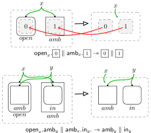
Figure 4: The open reaction rule of the Ambient Calculus (top) and an induced reaction.

2.2 Bigraph embeddings

The following definitions are mainly taken from [9], with minor modification to simplify the presentation of the distributed embedding algorithm (cf. Section 5). As usual, we will exploit the orthogonality of the link and place graphs, by defining link and place graph embeddings separately and then combine them to extend the notion to bigraphs.

Link graph

Intuitively an embedding of link graphs is a structure preserving map from one link graph (the guest) to another (the host). As one would expect from a graph embedding, this map contains a pair of injections: one for the nodes and one for the edges (i.e., a support translation). The remaining of the embedding map specifies how names of the inner and outer interfaces should be mapped into the host link graph. Outer names can be mapped to any link; here injectivity is not required since a context can alias outer names. Dually, inner names can mapped to hyper-edges linking sets of points in the host link graph and such that every point is contained in at most one of these sets.

Definition 2 (Link graph embedding [9, Def 7.5.1]).

Let $G:X_{G}\to Y_{G}$ and $H:X_{H}\to Y_{H}$ be two concrete link graphs. A link graph embedding $\phi:G\mathbin{\leavevmode\hbox to10.01pt{\vbox to4.48pt{\text{[drawing]}}}}H$ is a map $\phi\triangleq\phi^{\mathsf{v}}\uplus\phi^{\mathsf{e}}\uplus\phi^{\mathsf{i}}\uplus\phi^{\mathsf{o}}$ (assigning nodes, edges, inner and outer names respectively) subject to the following conditions:

(LGE-1)

$\phi^{\mathsf{v}}:V_{G}\rightarrowtail V_{H}$ and $\phi^{\mathsf{e}}:E_{G}\rightarrowtail E_{H}$ are injective;

(LGE-2)

$\phi^{\mathsf{i}}:X_{G}\rightarrowtail\wp(X_{H}\uplus P_{H})$ is fully injective: $\forall x\neq x^{\prime}:\phi^{\mathsf{i}}(x)\cap\phi^{\mathsf{i}}(x^{\prime})=\emptyset$;

(LGE-3)

$\phi^{\mathsf{o}}:Y_{G}\to E_{H}\uplus Y_{H}$ in an arbitrary partial map;

(LGE-4)

$\textsf{{img}}(\phi^{\mathsf{e}})\cap\textsf{{img}}(\phi^{\mathsf{o}})=\emptyset$ and $\textsf{{img}}(\phi^{\mathsf{port}})\cap\bigcup\textsf{{img}}(\phi^{\mathsf{i}})=\emptyset$;

(LGE-5)

$\phi^{\mathsf{p}}\circ{\left.\kern-1.2pt\textsf{{link}}_{G}^{-1}\vphantom{\big{|}}\right|_{E_{G}}}=\textsf{{link}}_{H}^{-1}\circ\phi^{\mathsf{e}}$;

(LGE-6)

$\textsf{{ctrl}}_{G}=\textsf{{ctrl}}_{H}\circ\phi^{\mathsf{v}}$;

(LGE-7)

$\forall p\in X_{G}\uplus P_{G}:\forall p^{\prime}\in(\phi^{\mathsf{p}})(p):(\phi^{\mathsf{h}}\circ\textsf{{link}}_{G})(p)=\textsf{{link}}_{h}(p^{\prime})$

where $\phi^{\mathsf{p}}\triangleq\phi^{\mathsf{i}}\uplus\phi^{\mathsf{port}}$, $\phi^{\mathsf{h}}\triangleq\phi^{\mathsf{e}}\uplus\phi^{\mathsf{o}}$ and $\phi^{\mathsf{port}}:P_{G}\rightarrowtail P_{H}$ is $\phi^{\mathsf{port}}(v,i)\triangleq(\phi^{\mathsf{v}}(v),i))$.

The first three conditions are on the single sub-maps of the embedding. Condition (LGE-4) ensures that no components (except for outer names) are identified; condition (LGE-5) imposes that points connected by the image of an edge are all covered. Finally, (LGE-6) and (LGE-7) ensure that the guest structure is preserved i.e. node controls and point linkings are preserved.

Place graph

Like link graph embeddings, place graph embeddings are just a structure preserving injective map from nodes along with suitable maps for the inner and outer interfaces. In particular, a site is mapped to the set of sites and nodes that are “put under it” and a root is mapped to the host root or node that is “put over it” splitting the host place graphs in three parts: the guest image, the context and the parameter (which are above and below the guest image).

Definition 3 (Place graph embedding [9, Def 7.5.4]).

Let $G:n_{G}\to m_{G}$ and $H:n_{H}\to m_{H}$ be two concrete place graphs. A place graph embedding $\phi:G\mathbin{\leavevmode\hbox to9.01pt{\vbox to0.4pt{\text{[drawing]}}}}H$ is a map $\phi\triangleq\phi^{\mathsf{v}}\uplus\phi^{\mathsf{s}}\uplus\phi^{\mathsf{r}}$ (assigning nodes, sites and regions respectively) subject to the following conditions:

(PGE-1)

$\phi^{\mathsf{v}}:V_{G}\rightarrowtail V_{H}$ is injective;

(PGE-2)

$\phi^{\mathsf{s}}:n_{G}\rightarrowtail\wp(n_{H}\uplus V_{H})$ is fully injective;

(PGE-3)

$\phi^{\mathsf{r}}:m_{G}\to V_{H}\uplus m_{H}$ in an arbitrary map;

(PGE-4)

$\textsf{{img}}(\phi^{\mathsf{v}})\cap\textsf{{img}}(\phi^{\mathsf{r}})=\emptyset$ and $\textsf{{img}}(\phi^{\mathsf{v}})\cap\bigcup\textsf{{img}}(\phi^{\mathsf{s}})=\emptyset$;

(PGE-5)

$\forall r\in m_{G}:\forall s\in n_{G}:\textsf{{prnt}}_{H}^{*}\circ\phi^{\mathsf{r}}(r)\cap\phi^{\mathsf{s}}(s)=\emptyset$;

(PGE-6)

$\phi^{\mathsf{c}}\circ{\left.\kern-1.2pt\textsf{{prnt}}_{G}^{-1}\vphantom{\big{|}}\right|_{V_{G}}}=\textsf{{prnt}}_{H}^{-1}\circ\phi^{\mathsf{v}}$;

(PGE-7)

$\textsf{{ctrl}}_{G}=\textsf{{ctrl}}_{H}\circ\phi^{\mathsf{v}}$;

(PGE-8)

$\forall c\in n_{G}\uplus V_{G}:\forall c^{\prime}\in\phi^{\mathsf{c}}(c):(\phi^{\mathsf{f}}\circ\textsf{{prnt}}_{G})(c)=\textsf{{prnt}}_{H}(c^{\prime})$;

where $\textsf{{prnt}}_{H}^{*}(c)=\bigcup_{i<\omega}\textsf{{prnt}}^{i}(c)$, $\phi^{\mathsf{f}}\triangleq\phi^{\mathsf{v}}\uplus\phi^{\mathsf{r}}$, and $\phi^{\mathsf{c}}\triangleq\phi^{\mathsf{v}}\uplus\phi^{\mathsf{s}}$.

Conditions in the above definition follows the structure of Definition 2, the main notable difference is (PGE-5) which states that the image of a root cannot be the descendant of the image of another. Conditions (PGE-1), (PGE-2) and (PGE-3) are on the three sub-maps composing the embedding; conditions (PGE-4) and (PGE-5) ensure that no components are identified; (PGE-6) imposes surjectivity on children and the last two conditions require the guest structure to be preserved by the embedding map.

Bigraph

Finally, bigraph embeddings can now be defined as maps being composed by an embedding for the link graph with one for the place graph consistently with the interplay of these two substructures. In particular, the interplay is captured by a single additional condition ensuring that points in the image of an inner names reside in the parameter defined by the place graph embedding (i.e. are inner names or ports of some node under a site image).

Definition 4 (Bigraph embedding [9, Def 7.5.14]).

Let $G:\langle n_{G},X_{G}\rangle\to\langle m_{G},Y_{G}\rangle$ and $H:\langle n_{H},X_{H}\rangle\to\langle m_{H},Y_{H}\rangle$ be two concrete bigraphs. A bigraph embedding $\phi:G\mathbin{\leavevmode\hbox to9.01pt{\vbox to0.4pt{\text{[drawing]}}}}H$ is a map given by a place graph embedding $\phi^{\mathsf{P}}:G^{P}\mathbin{\leavevmode\hbox to9.01pt{\vbox to0.4pt{\text{[drawing]}}}}H^{P}$ and a link graph embedding $\phi^{\mathsf{L}}:G^{L}\mathbin{\leavevmode\hbox to9.01pt{\vbox to0.4pt{\text{[drawing]}}}}H^{L}$ subject to the consistency condition:

(BGE-1)

$\textsf{{img}}(\phi^{\mathsf{i}})\subseteq X_{H}\uplus\{(v,i)\in P_{H}\mid\exists s\in n_{G}:k\in\mathbb{N}:\textsf{{prnt}}_{H}^{k}(v)\in\phi^{\mathsf{s}}(s)\}$.

3 Partial and candidate partial bigraph embeddings

In this Section we introduce the notion of partial bigraph embeddings. We show that for a given pair of guest and host bigraphs, the set of their partial embeddings is endowed with a “almost atomic” meet-semilattice. This structure will play a central rôle in the algorithm presented in Section 5. We then consider also the situation when we know only a part of the codomain of a partial embedding, by introducing the notion of candidate partial embedding.

3.1 Partial bigraph embeddings

Basically, a partial bigraph embedding is a partial map subject to the same conditions of a total embedding (Definition 4) up-to partiality.

Definition 5 (Partial bigraph embedding).

Let $G:\langle n_{G},X_{G}\rangle\to\langle m_{G},Y_{G}\rangle$ and $H:\langle n_{H},X_{H}\rangle\to\langle m_{H},Y_{H}\rangle$ be two concrete bigraphs. A partial bigraph embedding $\phi:G\mathbin{\leavevmode\hbox to10.01pt{\vbox to1.8pt{\text{[drawing]}}}}H$ is a partial map subject, where defined, to the same conditions of Definition 4.

As we will see in Section 5, partial embeddings represent the partial or intermediate steps towards a total embedding. This notion of “approximation” is reflected by the obvious ordering given by the point-wise lifting of the anti-chain order to partial maps. In particular, given two partial embeddings $\phi,\psi:G\mathbin{\leavevmode\hbox to9.01pt{\vbox to0.4pt{\text{[drawing]}}}}H$ we say that:

$$\phi\sqsubseteq\psi\stackrel{{\scriptstyle\triangle}}{{\iff}}\forall x\in\textsf{{dom}}(\phi)\,\phi(x)\neq\perp\implies\psi(x)=\phi(x)\text{.}$$ (1)

This definition extends, for any given pair of concrete bigraphs $G$ and $H$, to a partial order over the set of partial bigraph embeddings of $G$ into $H$. It is easy to check that the entirely undefined embedding $\varnothing$ is the bottom of this structure and that meets are always defined:

$$\phi\sqcap\psi\triangleq\lambda x.\begin{cases}\phi(x)&\text{if }\phi(x)=\psi(x)\\ \perp&\text{otherwise}\end{cases}$$

Likewise, joins, where they exist, are defined as follows:

$$\phi\sqcup\psi\triangleq\lambda x.\begin{cases}\phi(x)&\text{if }\phi(x)\neq\perp\\ \psi(x)&\text{if }\psi(x)\neq\perp\\ \perp&\text{otherwise}\end{cases}$$

Clearly $\phi$ and $\psi$ have to coincide where are both defined and their join $\phi\sqcup\psi$ is defined iff it does not violate any condition in Definition 5.

The set of partial embeddings for a given guest $G$ and host $H$ is an meet-semilattice. Moreover, an embedding can be represented as the meet of a finite set of “basic” elementary partial embeddings, i.e. suitable elements from $G\times H$. This suggests to use these elementary partial embeddings as a compact representation for (partial) embeddings. Although elementary partial embeddings may remind atomic elements in meet-semilattices, they are not really atomic. In fact, a partial embedding whose domain contains a site (or an inner name) has to map it to the empty-set in order to be minimal (and hence an atom); for this reason, a partial embedding mapping a site to something different than $\emptyset$ could not be described as the join of atoms.

This observation leads us to introduce the following definition.

Definition 6 ((Almost) atomic partial embedding).

A partial embedding $\alpha:G\mathbin{\leavevmode\hbox to9.01pt{\vbox to0.4pt{\text{[drawing]}}}}H$ is said to be (almost) atomic whenever the following implication holds true:

$$\psi\sqsubseteq\alpha\implies\psi=\varnothing\lor\exists!s\in n_{G}\uplus X_{G}.\psi(s)=\emptyset\text{.}$$

The set of atoms below a partial embedding $\phi$ is called base of $\phi$ and is denoted as $At(\phi)$. The set of all atomic partial embeddings of $G$ into $H$ is denoted as $At_{G,H}$ (we shall drop the subscripts when confusion seems unlikely).

Proposition 1 (Base).

Let $\phi:G\mathbin{\leavevmode\hbox to9.01pt{\vbox to0.4pt{\text{[drawing]}}}}H$ be a partial embedding. There exists a minimal and finite family $At(\phi)$ of (almost) atomic partial embeddings whose join is $\phi$.

Proof.

Let $At(\phi)$ be the set of (almost) atomic partial embeddings given by the union of:

• $\left\{{\left.\kern-1.2pt\phi\vphantom{\big{|}}\right|_{u}}\,\middle|\,u\in V_{G}\uplus m_{G}\uplus E_{G}\uplus Y_{G}\right\}$,

• $\left\{{\left.\kern-1.2pt\phi\vphantom{\big{|}}\right|^{w}}\,\middle|\,u\in n_{G}\uplus X_{G}\land w\in\phi(u)\right\}$, and

• $\left\{{\left.\kern-1.2pt\phi\vphantom{\big{|}}\right|_{u}}\,\middle|\,u\in n_{G}\uplus X_{G}\land\phi(u)=\emptyset\right\}$

where ${\left.\kern-1.2pt\phi\vphantom{\big{|}}\right|^{w}}$ denotes co-restriction. Then $\bigsqcup At(\phi)=\phi$ and $\bigsqcup S\sqsubset\phi$ for any $S\subset At(\phi)$. ∎

3.2 Candidate partial embeddings

A candidate partial embedding is a partial map $\rho:G\rightharpoonup H$ with the same domain and codomain of an embedding of $G$ into $H$. A candidate embedding is a total map with suitable domain and codomain. Note that every candidate defined only on a single element is a partial embedding.

The notion of candidate partial embedding is accessory to the decentralized algorithm we presents in Section 5. In fact, families of partial embeddings are sent over the network as graphs whose vertexes are atoms and whose edges represents admissible joins. Joins are not transitive and some of the conditions of bigraph embeddings cannot be checked by only looking at pairs of atoms and their immediate neighbourhood, as we show in Theorem 2 and Theorem 3.

Before we present this result let us present (LGE-5) and (PGE-6) in a more convenient (but equivalent) form, that points out the conditions failing to be “locally verifiable”.

(LGE-5a)

$\forall e\in E_{G}\forall x\in P_{G}\uplus X_{G}(x\in\textsf{{link}}^{-1}_{G}(e)\iff\phi^{\mathsf{p}}(x)\subseteq\textsf{{link}}^{-1}_{H}(\phi^{\mathsf{e}}(e)))$

(LGE-5b)

$\forall e\in E_{G}\forall y\in\textsf{{link}}^{-1}_{H}(\phi^{\mathsf{e}}(e))\exists x\in P_{G}\uplus X_{G}(y\in\phi^{\mathsf{p}}(x))$

(PGE-6a)

$\forall v\in V_{G}\forall s\in n_{G}\uplus V_{G}(s\in\textsf{{prnt}}^{-1}_{G}(v)\iff\phi^{\mathsf{c}}(s)\subseteq\textsf{{prnt}}^{-1}_{H}(\phi^{\mathsf{e}}(v)))$

(PGE-6b)

$\forall v\in V_{G}\forall y\in\textsf{{prnt}}^{-1}_{H}(\phi^{v}(v))\exists s\in n_{G}\uplus V_{G}(y\in\phi^{c}(s))$

Theorem 2.

Let $\rho:G\to H$ be a candidate embedding and let $\alpha_{1},\dots,\alpha_{n}$ the atoms forming it. $\rho:G\to H$ satisfies conditions (LGE-1-5a,6,7) and (PGE-1-4,6a,7,8) if, and only if,

1. $\forall i$ $\alpha_{i}$ satisfies (LGE-3), (LGE-6), (PGE-3), and (PGE-7);

2. $\forall i,j$ s.t. the candidate $\alpha_{i}\sqcup\alpha_{j}$ satisfies (LGE-1,2,4,5a,7) and (PGE-1,2,4,6a,8);

and each check involves at most the components of $H$ adjacent to the image of $\alpha_{i}$ and $\alpha_{j}$.

Proof (Sketch).

Its easy the above conditions can be falsified by providing at most two atoms and that the negated formula of each condition involves at most one step along $\textsf{{prnt}}_{H}$ or $\textsf{{link}}_{H}$. As an example we detail the case of (LGE-5a) leaving the others to the reader. If $\rho$ does not satisfy (LGE-5a), then there are $e\in E_{G}$ and $x\in P_{G}\uplus X_{G}$ s.t.:

$$(x\in\textsf{{link}}^{-1}_{G}(e)\land\rho^{\mathsf{p}}(x)\not\subseteq\textsf{{link}}^{-1}_{H}(\rho^{\mathsf{e}}(e)))\lor(x\not\in\textsf{{link}}^{-1}_{G}(e)\land\rho^{\mathsf{p}}(x)\subseteq\textsf{{link}}^{-1}_{H}(\rho^{\mathsf{e}}(e))) \dagger$$ ()

Let $\bar{e}\in E_{G}$ and $\bar{x}\in P_{G}\uplus X_{G}$ two witnesses of ($\dagger$ ‣ 3.2) and consider the atomic partial embeddings $\alpha_{1}={\left.\kern-1.2pt\rho\vphantom{\big{|}}\right|^{\bar{e}}}$ and $\alpha_{2}={\left.\kern-1.2pt\rho\vphantom{\big{|}}\right|^{\bar{x}}}$. Clearly $\alpha_{1},\alpha_{2}\sqsubseteq\rho$ and either $\bar{x}\in\textsf{{link}}^{-1}_{G}(\bar{e})\land\bar{y}\not\in\textsf{{link}}^{-1}_{H}(\bar{d})$ or $\bar{x}\not\in\textsf{{link}}^{-1}_{G}(\bar{e})\land\bar{y}\in\textsf{{link}}^{-1}_{H}(\bar{d})$. ∎

Theorem 3.

Verifying whether a candidate satisfies conditions (BGE-1), (LGE-5b), (PGE-5) and (PGE-6b) may require more than two atoms or the neighbourhood of their images.

Proof (Sketch).

Conditions (PGE-5) and (BGE-1) contain the transitive closure of $\textsf{{prnt}}_{H}$. Conditions (LGE-5b) and (PGE-6b) contain existential and universal quantifications at the same time. ∎

Definition 7.

Conditions (LGE-1-5a,6,7) and (PGE-1-4,6a,7,8) are called locally checkable, and the candidates satisfying them are said locally checked. Conditions (PGE-5) and (BGE-1) are called ancestor checkable, and the candidates satisfying them are said ancestor checked.

4 State, overlay and reactions

This section illustrates how a bigraph is distributed between a processes family and how it is maintained and updated. First, we formalize the idea of a “distributed bigraph” and show how a partition of the global system state defines a semantic overlay network. The rôle of this network is crucial for the embedding algorithm since communication will follow this structure. Finally, we describe how reactions are carried out concurrently and consistently.

In the following, let $\mathsf{Proc}$ denote the family of processes forming the distributed bigraphical machine under definition and let $H$ be a generic concrete bigraph $(V_{H},E_{H},\textsf{{ctrl}}_{H},\textsf{{prnt}}_{H},\textsf{{link}}_{H}):\langle n_{H},X_{H}\rangle\to\langle m_{H},Y_{H}\rangle$ over a given signature $\Sigma$.

4.1 State partition

Intuitively, a partition of the shared state $H$ is a map assigning each component of the bigraph $H$ to the process in charge of maintaining it.

Definition 8 (State partition).

A partition of (the shared state) $H$ over $\mathsf{Proc}$ is a map $\mathbb{P}:H\to\mathsf{Proc}$ assigning each component of $H$ to some process. In particular, $\mathbb{P}$ is given by the (sub)maps $\mathbb{P}^{\mathsf{\kern 1.0ptv}}$, $\mathbb{P}^{\mathsf{\kern 1.0pte}}$, $\mathbb{P}^{\mathsf{\kern 1.0pts}}$, $\mathbb{P}^{\mathsf{\kern 1.0ptr}}$, $\mathbb{P}^{\mathsf{\kern 1.0pti}}$, and $\mathbb{P}^{\mathsf{\kern 1.0pto}}$ on vertices, edges, sites, roots, inner names, and outer names respectively. Every component of $H$ in the pre-image of a process is said to be held by or local to that process. Ports are mapped into the process holding their node i.e. $\mathbb{P}((v,i))\triangleq\mathbb{P}(v)$.

State partitions define a notion of locality or ownership for bigraphs distributed across the given family of processes by a partition. This notion extends directly to embeddings.

Definition 9 (Local partial embedding).

Let $\phi:G\mathbin{\leavevmode\hbox to9.01pt{\vbox to0.4pt{\text{[drawing]}}}}H$ be a partial embedding and let $\mathbb{P}:H\to\mathsf{Proc}$ be a partition. The owners of $\phi$ are the processes in $\textsf{{img}}(\mathbb{P}\circ\phi)$. If $\phi$ has exactly one owner then it is said to be local to it. We denote the restriction of $\phi$ to the portion of bigraph held by a set of processes $S\subseteq\mathsf{Proc}$ as ${\left.\kern-1.2pt\phi\vphantom{\big{|}}\right|_{\mathbb{P},S}}$; we shall drop the partition $\mathbb{P}$ when confusion seems unlikely.

Given a process $Q$, every partial embedding $\psi\sqsubseteq{\left.\kern-1.2pt\phi\vphantom{\big{|}}\right|_{\mathbb{P},\{Q\}}}$ is local to $Q$–except for the undefined embedding $\varnothing$ since the set $\textsf{{img}}(\mathbb{P}\circ\varnothing)$ will always be empty. Therefore, the set of atoms below the restriction of $\phi$ to $Q$

$$At\left({\left.\kern-1.2pt\phi\vphantom{\big{|}}\right|_{\{Q\}}}\right)=\left\{\alpha\in At\,\middle|\,\alpha\sqsubseteq{\left.\kern-1.2pt\phi\vphantom{\big{|}}\right|_{\{Q\}}}\right\}$$

can be thought as the support of $\phi$ local to $Q$; any change in the bigraph held by $Q$ that affects one of these atoms will necessarily invalidate $\phi$. This last observation is at the hearth of the retraction phase of the embedding algorithm (cf. Section 5).

The notion of adjacency for bigraph components lifts to the family of processes along the given partition map. Here hyper-edges of the link graph are considered as trees where the root is the hyper-edge handle (i.e. an edge or an outer name) and leaves are all the points (i.e. ports or inner names) it connects.

Definition 10.

Let $Q,R\in\mathsf{Proc}$. The process $Q$ is said to be adjacent (w.r.t. the partition $\mathbb{P}$) to $R$ whenever one of the following holds:

(ADJ-P)

there exists a node, port or site $c$ s.t. $\mathbb{P}(c)=Q$ and $\mathbb{P}(\textsf{{prnt}}_{H}(c))=R$;

(ADJ-L)

there exists a point $p$ s.t. $\mathbb{P}(p)=Q$ and $\mathbb{P}(\textsf{{link}}_{H}(p))=R$;

(ADJ-T)

there exist two roots or handles $t,t^{\prime}$ s.t. $\mathbb{P}(t)=Q$ and $\mathbb{P}(t^{\prime})=R$;

A partial embedding $\phi$ is said to be adjacent to a process $R$ (w.r.t. $\mathbb{P}$) iff its image is. Adjacency of $Q$ or $\phi$ to $R$ w.r.t. $\mathbb{P}$ is denoted by ${Q\stackrel{{\scriptstyle\raisebox{-6.02777pt}{$\scriptscriptstyle\,\mathbb{P}$}}}{{\mathrel{{\circ}\!{\to}}}}R}$ and ${\phi\stackrel{{\scriptstyle\raisebox{-6.02777pt}{$\scriptscriptstyle\,\mathbb{P}$}}}{{\mathrel{{\circ}\!{\to}}}}R}$ respectively (with the option to from $\mathbb{P}$ when confusion no confusion may arise).

The adjacency relation defines a directed graph with vertices in $\mathsf{Proc}$ and hence a directed overlay network $\mathsf{N}_{\mathbb{P}}$. This network bares a specific semantic meaning because it reflects adjacency of the bigraphical elements held by each process forming the network: two processes are adjacent if, and only if, they hold components that are adjacent in the distributed bigraph $H$. The network $\mathsf{N}_{\mathbb{P}}$ is such that shortest paths connecting processes in it cannot exceed in length shortest paths between the components of $H$ they hold.

Lemma 4.

Let $c_{1},c_{2}\in H$. The length of shortest path in $\mathsf{N}_{\mathbb{P}}$ connecting $\mathbb{P}(c_{1})$ and $\mathbb{P}(c_{2})$ is limited from above ed by the length of the shortest path in $H$ connecting $c_{1}$ and $c_{2}$.

Proof (sketch).

Definition 10 characterizes the quotient induced by $\mathbb{P}$ on $H$. ∎

The last observation is crucial to our purposes since relates routing through the overlay $\mathsf{N}_{\mathbb{P}}$ with walks and visits of $H$ used e.g. to compute embeddings into $H$ in non-distributed settings. Notice that the restriction of $\mathsf{N}_{\mathbb{P}}$ to $\textsf{{img}}(\mathbb{P})$ will always be connected i.e. for any two processes in $\textsf{{img}}(\mathbb{P})$ there (at least) two paths starting from them and ending in the same node. This ensures that there is always a “rendezvous” point for two messages (and in particular two partial embeddings to be combined). Connectedness is ensured by (ADJ-T) but this condition is sufficient and can be relaxed by assuming the adjacency relation to contain a directed-complete partial order (dCPO) on $\textsf{{img}}(\mathbb{P})$. Note that each process is aware to its neighbouring processes and the nature of their adjacency because each process knows parents, children, etc. of each component it hold.

Remark 1.

In [13] we considered, for the sake of simplicity, an undirected graph as overlay network. However, the additional information of a directed overlay network allows for more efficient routing strategies hence reducing duplicated computations of partial embeddings (cf. Section 5). In fact, edge direction reflects the structure of the bigraph and can be leveraged also by partition strategies to distribute the bigraph privileging locality of reactions.

Example 2 (Multi-Agent Systems).

In [12] we described how BRS can be used to both design and prototype multi-agent systems (MAS). In loc. cit. BRS are used to model the application domain lending helpful formal verification tools (e.g. model checkers) to the designer as long as simulation ones. Then entities forming each bigraph are divided as subjects and objects accordingly to their rôle in the model (e.g. node controls); with the former being the agents in the systems. When agents are identified with processes of a D-BAM this yield a prototype of the system where agent cooperation and reconfiguration correspond to negotiation of execution strategies and reactions respectively.

In [12] each entity designated as object (e.g. a node modelling a good) is assigned to the process of its first ancestor designated as a subject (e.g. a node modelling a store). This is an instance of partition strategy. In particular, the partition is driven by the application domain privileging locality of interactions: a store is going to be involved by each reaction affecting its goods.

4.2 Distributed reactions

Let $\phi$ be an embedding of $G$ into the bigraph $H$ distributed across the processes in the system and let $r:G\rightarrowtriangle G^{\prime}$ be a parametric rewriting rule for the given BRS. Processes holding elements of $G$ image through $\phi$ or in its parameters have to negotiate the firing of $r$ and coordinate the update of their state. The negotiation phase is related to the specific execution policy and hence is left out from the present work (see [12, 18] for an example). The update phase involves a distributed transaction is handled by established algorithms like two-phase-commit [5].

Each process concurrently enacts two roles: one active and one passive. In the first case: (1a) it selects a reaction (e.g.-rewriting rule, edit script) and a suitable embedding among those provided by its embedding engine; (1b) starts a transaction with all the processes involved in the embedding (i.e. $\textsf{{img}}(\mathbb{P}\circ\phi)$); (1c) waits for them to either approve or reject the reaction and completes the transaction protocol accordingly. In the second case: (2a) it waits for other processes to propose a reaction; (2b) votes for acceptance or rejection (execution strategy); (2c) executes the reaction iff each other participant agrees on committing the transaction. Note that consistency of the current bigraph is guaranteed by the correctness of the distributed transaction protocol, even in presence of outdated embeddings or concurrent transactions.

In [12] reactions correspond to agent reconfigurations. These may result in agent creation or termination requiring a life-cycle for processes of the D-BAM too–since the latter are identified with the former. Although we assumed a fixed family of processes, to simplify the exposition, the D-BAM supports churns that are contextual to reactions, especially when partitions are implicitly adapted by partition strategies of the like of [12].

5 Distributed embedding

In this Section we introduce a decentralized algorithm for computing bigraphical embeddings in the distributed settings outlined in Section 4 and Figure 3. Intuitively, each process running this algorithm maintains a private collection of partial embeddings for the guests it has to look for and cooperates with its neighbouring processes to complete or refute them.

For the sake of simplicity we assume that all processes are given the same set of guests (e.g. the redexes of parametric rewriting rules defining the BRS being executed by the D-BAM), that this set is fixed over the time and does not contain the empty bigraph. However, these mild assumptions can be dropped with minor changes to the algorithm. Likewise, we assume causally ordered communication and refer the reader to [13] for a version of the algorithm where message causality and group communication are explicitly implemented on reliable point-to-point channels by means suitable logical clocks (i.e. internal counters that every process attach to the information it generates).

5.1 Computing and updating partial embedding

Each process $Q$ in the D-BAM executes the embedding engine module alongside the reaction engine (cf. Figure 3) with which it asynchronously communicates by means of shared state structures. On one side, the module observes the chunk of the current bigraph held by the process and the updates the reaction module commits on it; this defines the input of the reaction engine. (Note that overlay network $\mathsf{N}_{\mathbb{P}}$ are implicitly and consistently updated during each distributed transaction wrapping a reaction.) On the other side, the module provides a collection of available embeddings i.e. a partial view of all the embeddings computed by the machine. This defines the output of the module. Although processes often have an incomplete view, the algorithm guarantees that each embedding is computed by at least one of them.

Reactions may invalidate embeddings which then have to be collected by this module. Each embedding engine operates on its local collection of available embeddings by means of two procedures: $\textnormal{{addEmbedding}}(\phi)$ and $\textnormal{{removeEmbeddings}}(\Psi)$ where the second removes all embeddings $\phi$ s.t. $\psi\sqsubseteq\phi$ for some $\psi\in\Psi$. High consistency of available embeddings collections is not mandatory (reactions are consistent) allowing us to trade some of it for performance and adopt an asynchronous garbage collection scheme for sweeping invalidated embeddings.

An embedding may be owned by more than one process forcing their execution engines to exchange information in order to compute/invalidate it. The data being exchanged consists of suggestions or retractions of partial embeddings and is conveyed by two kind of messages: suggest and retract. The former kind push newly discovered partial embeddings to other processes and the latter propagate invalidations. For efficiency reasons, partial embeddings are sent in batches encoded as irreflexive undirected graphs (called atom graphs) whose nodes are the atoms composing them (cf. Proposition 1) and whose edges are checkable joins in the sense of Theorem 2. Atom graphs implicitly describe candidates but, by Theorem 3 embeddings cannot be singled out without looking at more than two atoms or their images; information that is available at suitable stages of the algorithm only.

The same encoding is used by each process to store the set of (candidate) partial embeddings forming its partial view of those existing in the system. To simplify the exposition we assume this structure as indexed over the set of guests (hence duplicating information relative to their overlaps). We shall denote this structure by $\Gamma_{Q,G}$, where $Q$ is the owning process and $G$ is the guest bigraph, and drop the subscripts when clear from the context. Each process $Q$ implicitly keeps track of which processes it received an atom from; this set will be denoted as $\mathsf{src}_{Q}(\alpha)$.

Event handler onRetract($G$, $RA$, $RE$)

      $(A,E)\leftarrow\Gamma_{Q,G}$

      $(A^{\prime},E^{\prime})\leftarrow(A\setminus RA,E\setminus RE)$

      if $A\not=A^{\prime}\lor E\not=E^{\prime}$ then

           $\Gamma_{Q,G}\leftarrow(A^{\prime},E^{\prime})$

           removeEmbeddings($RA\cup\{\alpha\sqcup\alpha^{\prime}|\{\alpha,\alpha^{\prime}\}\in RE\}$)

           send retract $\langle G,RA,RE\rangle$ to $\{P\mid{Q\mathrel{{\circ}\!{\to}}P}\}$

           end if

          

          

Algorithm 1

Event handler onSuggest($G$, $A^{\prime}$, $E^{\prime}$)

      $(A,E)\leftarrow\Gamma_{Q,G}$

      $A^{\prime\prime}\leftarrow A\cup A^{\prime}$

      $E^{\prime\prime}\leftarrow E\cup E^{\prime}\cup${$\{\alpha,\alpha^{\prime}\}\mid\alpha\sqcup\alpha^{\prime}\in A\bigsqcup A^{\prime}\text{ is \hyperref@@ii[def:locally-checkable]{locally checked} and \hyperref@@ii[def:ancestor-checkable]{ancestor checked}}$}

      if $A\not=A^{\prime\prime}\lor E\not=E^{\prime\prime}$ then

           $\Gamma_{Q,G}\leftarrow(A^{\prime\prime},E^{\prime\prime})$

           for $\phi\in\textnormal{{getCandidateEmbeddings(}}\textnormal{\emph{A'', E''}}\textnormal{{)}}$ do

                if $\phi$ satisfies (LGE-5b) and (PGE-6b) then

                     addEmbedding($\phi$)

                     end if

                    

                     end for

                     send suggest $\langle G,A^{\prime},E^{\prime}\rangle$ to $\{P\mid{Q\mathrel{{\circ}\!{\to}}P}\}$

                     end if

                    

                    

Algorithm 2

Writes on $\Gamma_{Q,G}$ are triggered by $Q$ receiving retract or suggest messages. The two events are handled by onRetract and onSuggest respectively. Retractions remove from $\Gamma_{Q,G}$ all invalidated atoms and edges–note that these are collections, not an actual graph. If any change is made the information if propagated to the neighbourhood of $Q$ and to the collection of available embeddings resulting in the removal of embeddings incoherent with the current bigraph $H$. Likewise suggestions add new atoms and locally checked joins to $\Gamma_{Q,G}$ being these edges in the message payload $E^{\prime}$ or computed by $Q$ from its view of the bigraph (recall that every process knows parents, children, etc. of every component it holds). Whenever changes to $\Gamma_{Q,G}$ are made, these are propagated to the process neighbourhood. Contextually, candidate embeddings (i.e. cliques in $\Gamma_{Q,G}$ whose atoms cover $G$ with their domains) are checked to single out any new embedding to be added to the collection of available ones. All locally and ancestor checkable conditions are encoded as edges leaving (LGE-5b) and (PGE-6b) to be checked right before executing addEmbedding. Ancestor checkable conditions require some extra care since the transitive closure of the place graph is involved. In general, processes have only a partial view of $\textsf{{prnt}}_{H}^{*}$ but this is sufficient under mild conditions on how atoms for roots, sites and inner names of $G$ routed. In fact, if this kind of atoms are travel along $\textsf{{prnt}}_{H}$ then, the least ancestor of their images (cf. Lemma 7) can check (PGE-5) and (BGE-1) by knowing the source of the message containing them (besides its atom graph and the one in the message).

Event handler onUpdate()

      for $G\in Guests$ do

           $(A,E)\leftarrow\Gamma_{Q,G}$

           $(A^{\prime},E^{\prime})\leftarrow$ getLocalAtoms(G)

           $RA\leftarrow\{\alpha\in A\setminus A^{\prime}\mid\textsf{{img}}(\mathbb{P}\circ\alpha)=\{Q\}\}$

           $RE\leftarrow$ $\{\{\alpha_{1},\alpha_{2}\}\in E\mid\alpha_{1}\in A\cap A^{\prime}\land(\alpha_{2}\in A\cap A^{\prime}\implies\{\alpha_{1},\alpha_{2}\}\notin E^{\prime})\}$

           send retract $\langle G,RA,RE\rangle$ to self

           waitOverlayUpdate()

           send suggest $\langle G,A^{\prime}\setminus A,E^{\prime}\setminus E\rangle$ to self

           end for

          

          

Algorithm 3

The mechanism offered by onRetract and onSuggest is also used by the event handler onUpdate to propagate the effect of reactions involving $Q$ to $\Gamma_{Q,G}$ and the rest of the system. The handler is triggered during the commit phase of any write to the partial view of the current bigraph owned by $Q$ and computes the “effect” of the write by looking for changes in the graph of atoms local to $Q$. The new graph can be computed applying the algorithm described in [15] (with minor adaptations to restrict the solution to atomic partial embeddings only). Then, the graph is compared to $\Gamma_{Q,G}$ (note that $\Gamma_{Q,G}$ may contain also atoms local to other processes) to find atoms and edges that have to be added or removed. Changes are passed to onRetract and onSuggest. Note that propagation of retracts to processes involved in the update has to be completed before any change to the overlay network is applied (i.e. between transaction commit approval and finalization) since this allows retracts to be dispatched along the same route of the atoms they are collecting. Concurrent reaction may still prevent every invalidated atom to be collected by this mechanism, however consistency of the machine state is still preserved by reactions being wrapped by distributed transaction. Another viable approach is offered by remote references and leasing times: atoms whose leasing is not renewed are considered retracted and automatically removed from the system. However, more messages would be exchanged in order to periodically renew leasing times.

5.2 Enhancements and heuristics

Routing

To simplify the presentation of the algorithm suggestions and retractions are sent indistinctly to the entire neighbourhood resulting in part of them being discarded by receivers. In particular, candidates that are not adjacent to a receiver are always discarded since the receiving process cannot contribute to or benefit from them in any way.

Therefore, atom graphs have to parted and dispatched only to those process adjacent to the candidates they describe. Formally, an atom graph is adjacent to a process whenever it can be covered by cliques each containing an atom adjacent to the process.

Definition 11.

An atom graph $(A,E)$ is said to be adjacent to a process $Q$ if, and only if, there exists a family of cliques $\{(A_{1},E_{1}),\dots,(A_{k},E_{k})\}$ such that:

• $(A,E)=\bigcup_{i}(A_{i},E_{i})$;

• there is $\alpha\in A_{i}$ s.t. $\alpha\mathrel{{\circ}\!{\to}}Q$ for each $1\leq i\leq k$;

• for each $\alpha\in A$, if $\textsf{{dom}}(\alpha)\in m_{G}\uplus n_{G}$ then $\alpha\mathrel{{\circ}\!{\to}}Q$.

Adjacency based routing is handled at the communication level, like causal ordering of messages. which sends to each recipient of a multicast send only the greatest sub-graph adjacent to it. Henceforth, we assume messages to be parted and dispatched following this routing protocol.

Isomorphisms

The network footprint of the algorithm suffers from combinatorics due to internal isomorphisms of guest and host bigraphs (cf. Theorem 11). Here we suggest an heuristic aimed to mitigate the impact of this phenomenon.

Consider the relation on atomic partial embeddings defined, for any two $\alpha,\beta\in At_{G,H}$, as:

$$\alpha\equiv\beta\stackrel{{\scriptstyle\triangle}}{{\iff}}\alpha\cong\beta\text{ and }\forall\gamma\in At_{G,H}\setminus\{\alpha,\beta\}\alpha\sqcup\gamma\iff\beta\sqcup\gamma$$

where $\alpha\cong\beta$ whenever there are two bigraph isomorphisms $\sigma_{G}$ and $\sigma_{H}$ s.t. $\alpha\circ\sigma_{G}=\sigma_{H}\circ\beta$. It is easy to check that this relation is an equivalence and hence defines quotients for atom graphs i.e. an effective compression for messages and, in general, structures based on atom graphs. A lossless compression requires atoms bo be decorated with their multiplicity (and any list of additional user provided properties often found in some extensions of bigraphs).

5.3 Adequacy

Reactions change the current bigraph and can be though as resetting the embedding engine with the latter then checking and updating its state coherently. Reworded, reactions are perturbations the embedding engine has to stabilize from and restoring the equilibrium produces traffic over the network. Traffic stops only when the equilibrium is reached i.e. the machine stabilizes.

Theorem 5 (Completeness).

When the system is stable, every embedding can be found in the collection of available embeddings of some process.

By causally ordered communication we can assume, w.l.o.g., that the system stabilized before the last reaction. Then completeness is equivalent to the fact that for each $\phi:G\mathbin{\leavevmode\hbox to9.01pt{\vbox to0.4pt{\text{[drawing]}}}}H$ there is some $Q$ s.t. $\phi\in(\Gamma_{Q,G})^{\star}$ where $(\Gamma_{Q,G})^{\star}$ is the set of partial embeddings whose atoms are in $\Gamma_{Q,G}$

Lemma 6.

If $\phi$ is a partial embedding for $G$ then there is a process $Q$ s.t. $\phi\in(\Gamma_{Q,G})^{\star}$.

Proof.

The proof is given by induction on the size of $\{Q_{1},\dots,Q_{k}\}=\textsf{{img}}(\mathbb{P}\circ\phi)$. If $k=1$ then the embedding is local to $Q_{1}$ and hence $\phi\in(\Gamma_{Q,G})^{\star}$. Otherwise, let $\phi_{i}={\left.\kern-1.2pt\{Q_{i}\}\vphantom{\big{|}}\right|_{\phi}}$ for $1\leq i\leq k$. By inductive hypothesis each $\phi_{i}\in(\Gamma_{Q_{i},G})^{\star}$. By connectedness hypothesis there is at least one process $Q$ reachable by each $Q_{i}$. Messages are routed to all, and only, the processes that can benefit from or contribute to them, in particular to $Q$. All edges that are locally checked and ancestor checked are added while messages travel the network. We only have to prove that there is always a process that can add each edge along the paths to $Q$. By Theorem 2, the only cases left are ancestor checkable. We conclude by Definition 11 and by Corollary 8. ∎

Lemma 7.

Let $r\in m_{G}$, $s\in n_{G}$, $\alpha:r\mapsto u$, $\alpha^{\prime}:s\mapsto\{u^{\prime}\}$ two atoms, and $v,v^{\prime}$ be the roots above $u$ and $u^{\prime}$ respectively. If $Q$ is the process to receive/compute $\alpha$ and $\alpha^{\prime}$ earlier then at least one of the following is true:

1. $Q$ holds the least ancestor of $u$ and $u^{\prime}$;

2. $Q$ holds both $v$ and $v^{\prime}$;

3. $Q$ holds either $v$ or $v^{\prime}$ and the process holding the other sent the embedding.

Let $i\in X_{G}$, $(u^{\prime\prime},p)\in V_{H}$, $1\leq p\leq\textsf{{ar}}\circ\textsf{{ctrl}}_{H}(u^{\prime\prime})$, and $\alpha^{\prime\prime}:i\mapsto\{(u^{\prime\prime},p)\}$. There is a process $Q$ that holds $u^{\prime}$ and an ancestor of $u^{\prime\prime}$.

Proof (Sketch).

Atoms for guest sites and roots are dispatched following $\textsf{{prnt}}_{H}$ only. Atoms for host ports are dispatched following both $\textsf{{prnt}}_{H}$ and $\textsf{{link}}_{H}$. ∎

Corollary 8 (Ancestor checks).

For any two ancestor checkable atoms involving host ports, guest roots or sites there is a process that computes their edge before the system stabilize.

Proof (Sketch).

The process receiving/computing the atoms for guest sites and roots earlier checks them by looking at his piece of the shared bigraph and at the adjacency witness used to dispatch the message (i.e. which child or sibling root was used by the sender process to route the message). Likewise, a process holding the image of a site checks whether a received inner name sits below it. ∎

Theorem 9 (Soundness).

If the system stabilizes then each embedding in the collection of available ones is valid w.r.t. the current bigraph.

Proof.

Effects of reactions are computed locally to each embedding engine and then propagated through the network. Propagation stops as soon as it stops producing changes in each $\Gamma$. By network connectedness and stabilization of the machine each invalid embedding is eventually computed and removed by onRetract. Embeddings are added only by onSuggest which filters out candidate and partial embeddings. ∎

5.4 Complexity

The arity of the set of all embeddings of $G$ into $H$ is in $\mathbf{O}(|G|^{|H|})$ since, in the worst case, guest and host encode two finite sets with a root for each element. On the other hand, by Proposition 1, the same set is described by families in $At_{G,H}$ or, following the representation used by the algorithm, by a suitable graph on $At_{G,H}$. Because elements of $At_{G,H}$ are essentially pairs from $G\times H$ the spatial complexity of the graph representation is in $\mathbf{O}(|G|^{2}\cdot|H|^{2})$ without any particular encoding. The same bound holds for the size of each message sent on the overlay network. However, a process sends over the network only nodes and edges it adds or removes from his $\Gamma_{G}$ and messages are dispatched on the base of their semantic adjacency. Therefore, between two reactions, every edge travels a link at most once (either inside a suggest or retract message).

Lemma 10.

The number of links in $\mathsf{N}_{\mathbb{P}}$ is in $\mathbf{O}(|H|)$.

Proof.

The number $L$ of links in $\mathsf{N}_{\mathbb{P}}$ is bounded by the size of $H$ since the $\mathsf{N}_{\mathbb{P}}$ is a quotient of $H$. Hence, the worst case network is $\mathsf{N}_{\mathbb{I}}$ where $\mathbb{I}:H\rightarrowtail\mathsf{Proc}$ is the finest possible partition (i.e each component is assigned a distinct process). Except for the clique induced by roots and handles, $\mathsf{N}_{\mathbb{I}}$ is a directed acyclic graph where each vertex has at most $1+\max_{v\in V_{H}}(\textsf{{ar}}\circ\textsf{{ctrl}}_{H})(v)$ outgoing edges and therefore is bounded by the maximal arity $k$ occurring the given signature $\Sigma$ which is a fixed parameter of the D-BAM, hence a constant. The remaining case is given by the clique of roots and handles; their outgoing degree may exceed $k$ but their topology can be easily reorganized to into a tree that satisfies the bound and the above reasoning. Therefore, $L$ is bounded by the number of components of $H$. ∎

The algorithm generates, in the worst case scenario, as much traffic as a centralized one in its best case scenario.

Theorem 11.

The traffic generated over $\mathsf{N}_{\mathbb{P}}$ while finding all the available embedding, between two reactions, is in $\mathbf{O}(|G|^{2}\cdot|H|^{3})$.

This scenario corresponds to bigraphs and partitions forcing information to traverse all the network. In fact, the algorithm sends atoms only to processes that can effectively benefit from it and hence their propagation is stopped as soon as possible while retaining correctness and completeness.

In a typical scenario guests are fixed over time (hence a constant) and $|H|$ outmatches $|G|$ by orders of magnitude. Moreover, embeddings unaffected by a reactions are not recomputed.

6 Conclusions and future work

In this paper we have presented a D-BAM, an abstract machine for executing BRSs in a distributed environment. The core novelty of this machine is an algorithm for computing bigraph embeddings in a distributed environment where the host bigraph is spread across several cooperating peers. Differently from existing algorithms [8, 15, 23], this one is completely decentralized and does not to have a complete view of the global state in any process in the system; hence it can scale to handle bigraphs too large to reside on a single process/machine.

As in any distributed system, the complexity of our algorithm is rendered by the number and the size of exchanged messages (i.e., the network footprint). On one hand, the number of messages needed for computing an embedding is linearly bounded by the size of the embedded bigraph (which usually is constant during execution) and the depth of the parent map of the host. The worst case (Theorem 11) is when the overlay network of processes is a list, and atoms have to traverse it entirely. This case happens for bigraphs and embeddings that can be seen as “pathological” in the context of BRS; this suggests to consider different encodings of the model into the BRS in order to improve locality of reactions. On the other hand, the size of messages depends on internal isomorphisms in the guest and host bigraphs: these symmetries yield a combinatorial explosion of the possible embeddings, leading to larger messages to be exchanged between processes. This is mitigated by the heuristics presented in Section 5.2. A possible future work is to perform a formal analysis of locality and isomorphisms and their impact in the context of smoothed complexity.

When a reaction is applied, it alters the distributed state and inherently invalidates some of the partial embeddings computed by each process. Consistency of the state is guaranteed by reactions being wrapped inside distributed transactions, but invalidated embeddings are an unnecessary burden. To this end, we used a retraction mechanisms as an asynchronous distributed garbage collection; moreover, embeddings that are not affected by a reaction are not recomputed. We think that this approach is a good trade-off between performance and consistency. In fact, other solutions can be implemented; for instance, invalidated embeddings can be collected during the reaction commit phase; this offers the highest consistency (the set of available embeddings will never contain invalid ones) at the cost of slower reactions. On the other extreme of the spectrum, invalidated embeddings are collected only when an inconsistency is found by some process. Reactions are as fast as in presence of asynchronous retractions but process data structures are heavily polluted by invalid embeddings resulting in a higher rate of aborted transactions i.e. failed reactions.

An interesting feature of the bigraphical framework is that, given a bigraph and a redex, we can calculate the minimal contexts (called IPOs) needed to complete the bigraph in order to match the given redex. Leveraging this property, a different, “semi-distributed” implementation of the bigraphical abstract machine has been proposed in [12]. According to this algorithm, a process willing to perform a rewrite has to (1) collect a (suitable) view of the host bigraph from its neighbour processes; (2) compute locally all the embeddings (i.e. all possible reactions for the given rewriting rule); (3) apply the execution policy and start a distributed rewriting inside a transaction. The existence of minimal contexts provide a bound to the view a process has to collect at step 1. However, this bound is outmatched by more substantial drawbacks, e.g.: parametric rules have to be expanded into ground ones beforehand, and each process may end up visiting (and copying) the entire bigraph. Hence, we think that the algorithm proposed in this paper outperformes the one in [12].

A direct application of the distributed embedding algorithm is to simulate, or execute, multi-agent systems. In [12] the authors propose a methodology for designing and prototyping multi-agent systems with BRSs. Intuitively, the application domain is modelled by a BRS and entities in its states are divided as “subjects” and “objects” depending on their ability to actively perform actions. Subjects are precisely the agents of the system and reactions are reconfigurations. This observation yields a coherent way to partition and distribute a bigraph among the agents, which can be assimilated to the processes of the distributed bigraphical machine (execution policies are defined by agents desires and goals). Therefore, these agents can find and perform bigraph rewritings in a truly concurrent, distributed fashion, by using the distributed embedding algorithm presented in this paper.

Finally, we observe that the performance of the algorithm (and hence of the D-BAM) depends on how the bigraph is partitioned and distributed. For instance, it is easy to devise a situation in which even relatively small guests require the cooperation of several processes, say nearly one for each component of the guest. An interesting line of research would be to study the relation between guests, partitions, and performance in order to develop efficient distribution strategies. Moreover, structured partitions lend themselves to ad-hoc heuristics and optimizations. As an example, the way bigraphs are distributed among agents in [12] takes into account of their interactions and reconfigurations.

References

- [1] G. Bacci, D. Grohmann, and M. Miculan. Bigraphical models for protein and membrane interactions. In G. Ciobanu, editor, Proc. MeCBIC, volume 11 of Electronic Proceedings in Theoretical Computer Science, pages 3–18, 2009.
- [2] G. Bacci, M. Miculan, and R. Rizzi. Finding a forest in a tree - the matching problem for wide reactive systems. In M. Maffei and E. Tuosto, editors, Proc. TGC, volume 8902 of Lecture Notes in Computer Science, pages 17–33. Springer, 2014.
- [3] L. Birkedal, S. Debois, E. Elsborg, T. Hildebrandt, and H. Niss. Bigraphical models of context-aware systems. In L. Aceto and A. Ingólfsdóttir, editors, Proc. FoSSaCS, volume 3921 of Lecture Notes in Computer Science, pages 187–201. Springer, 2006.
- [4] M. Bundgaard, A. J. Glenstrup, T. T. Hildebrandt, E. Højsgaard, and H. Niss. Formalizing higher-order mobile embedded business processes with binding bigraphs. In D. Lea and G. Zavattaro, editors, Proc. COORDINATION, volume 5052 of Lecture Notes in Computer Science, pages 83–99. Springer, 2008.
- [5] E. C. Cooper. Analysis of distributed commit protocols. In Proc. SIGMOD, pages 175–183. ACM, 1982.
- [6] T. C. Damgaard, E. Højsgaard, and J. Krivine. Formal cellular machinery. Electronic Notes in Theoretical Computer Science, 284:55–74, 2012.
- [7] A. J. Faithfull, G. Perrone, and T. T. Hildebrandt. BigRed: A development environment for bigraphs. ECEASST, 61, 2013.
- [8] A. Glenstrup, T. Damgaard, L. Birkedal, and E. Højsgaard. An implementation of bigraph matching. IT University of Copenhagen, 2007.
- [9] E. Højsgaard. Bigraphical Languages and their Simulation. PhD thesis, IT University of Copenhagen, 2012.
- [10] O. H. Jensen and R. Milner. Bigraphs and transitions. In A. Aiken and G. Morrisett, editors, POPL, pages 38–49. ACM, 2003.
- [11] J. Krivine, R. Milner, and A. Troina. Stochastic bigraphs. In Proc. MFPS, volume 218 of Electronic Notes in Theoretical Computer Science, pages 73–96, 2008.
- [12] A. Mansutti, M. Miculan, and M. Peressotti. Multi-agent systems design and prototyping with bigraphical reactive systems. In K. Magoutis and P. Pietzuch, editors, Proc. DAIS, volume 8460 of Lecture Notes in Computer Science, pages 201–208. Springer, 2014.
- [13] A. Mansutti, M. Miculan, and M. Peressotti. Towards distributed bigraphical reactive systems. In R. Echahed, A. Habel, and M. Mosbah, editors, Proc. GCM’14, page 45, 2014. Workshop version.
- [14] M. Miculan and M. Peressotti. Bigraphs reloaded: a presheaf presentation. Technical Report UDMI/01/2013, Dept. of Mathematics and Computer Science, Univ. of Udine, 2013.
- [15] M. Miculan and M. Peressotti. A CSP implementation of the bigraph embedding problem. In T. T. Hildebrandt, editor, Proc. MeMo, 2014. To appear.
- [16] R. Milner. The Space and Motion of Communicating Agents. Cambridge University Press, 2009.
- [17] E. Pereira, C. M. Kirsch, J. B. de Sousa, and R. Sengupta. BigActors: a model for structure-aware computation. In C. Lu, P. R. Kumar, and R. Stoleru, editors, ICCPS, pages 199–208. ACM, 2013.
- [18] G. Perrone. Domain-Specific Modelling Languages in Bigraphs. PhD thesis, IT University of Copenhagen, 2013.
- [19] G. Perrone, S. Debois, and T. T. Hildebrandt. Bigraphical refinement. In J. Derrick, E. A. Boiten, and S. Reeves, editors, Proc. REFINE, volume 55 of Electronic Proceedings in Theoretical Computer Science, pages 20–36, 2011.
- [20] G. Perrone, S. Debois, and T. T. Hildebrandt. A model checker for bigraphs. In S. Ossowski and P. Lecca, editors, Proc. SAC, pages 1320–1325. ACM, 2012.
- [21] G. Rozenberg, editor. Handbook of graph grammars and computing by graph transformation, volume 1. World Scientific, River Edge, NJ, USA, 1997.
- [22] M. Sevegnani and E. Pereira. Towards a bigraphical encoding of actors. In T. T. Hildebrandt, editor, Proc. MeMo, 2014. To appear.
- [23] M. Sevegnani, C. Unsworth, and M. Calder. A SAT based algorithm for the matching problem in bigraphs with sharing. Technical Report TR-2010-311, Department of Computer Science, University of Glasgow, 2010.