On a non-homogeneous and non-linear heat equation.

Abstract.

We consider the Cauchy-problem for a parabolic equation of the following type:

$$\frac{\partial u}{\partial t}=\Delta u+f(u,|x|),$$

where $f=f(u,|x|)$ is supercritical. We supply this equation by the initial condition $u(x,0)=\phi$, and we allow $\phi$ to be either bounded or unbounded in the origin but smaller than stationary singular solutions. We discuss local existence and long time behaviour for the solutions $u(t,x;\phi)$ for a wide class of non-homogeneous non-linearities $f$. We show that in the supercritical case, Ground States with slow decay lie on the threshold between blowing up initial data and the basin of attraction of the null solution. Our results extend previous ones allowing Matukuma-type potential and more generic dependence on $u$.

Then, we further explore such a threshold in the subcritical case too. We find two families of initial data $\zeta(x)$ and $\psi(x)$ which are respectively above and below the threshold, and have arbitrarily small distance in $L^{\infty}$ norm, whose existence is new even for $f(u,r)=u^{q-1}$. Quite surprisingly both $\zeta(x)$ and $\psi(x)$ have fast decay (i.e. $\sim|x|^{2-n}$), while the expected critical asymptotic behavior is slow decay (i.e. $\sim|x|^{2/q-2}$).

Key Words: Cauchy-problem, semi-linear heat equation, singular solutions,
stability.
MSC (2010):   35k80, 35b60, 35b40

1. Introduction

The purpose of this paper is to study the asymptotic behavior of positive solutions of the following Cauchy problem

(1.1) $$\frac{\partial u}{\partial t}=\Delta u+f(u,|x|),$$

(1.2) $$u(x,0)=\phi(x),$$

where $x\in{\mathbb{R}}^{n}$, $n>2$, and $f=f(u,|x|)$ is a potential which is null for $u=0$.

In the last 20 years this problem has raised a great interest, starting from the model cases $f(u,|x|)=u^{q-1}$ and $f(u,|x|)=|x|^{\delta}u^{q-1}$. Due to symmetry reasons, from now on we use notations which are standard for the stationary problem, so we refer to $f(u,|x|)=u^{q-1}$ as the model case. In so doing it will be more clear the relationship between the critical values for (1.7) appearing below, and their meaning in other contexts of functional analysis.

We assume that $f$ is supercritical with respect to the Serrin critical exponent, i.e. $2_{*}:=\frac{2(n-1)}{n-2}$, and for some specific results we require $f$ to be supercritical also to the Sobolev critical exponent, i.e. $2^{*}:=\frac{2n}{n-2}$. The exponents $2_{\ast}$ and $2^{\ast}$ are related to the continuity of the trace operator in $L^{q}$ and to the possibility to embed $H^{1}$ in $L^{q}$, respectively.

Here, we want to analyze the structure of the border of the basin of attraction to the null solutions, and the set of initial data $\phi$ of solutions of (1.1)–(1.2) which blow up in finite time. Our main aim is to extend the discussion to a wide class of potentials: For the remainder of the paper we will always assume the following

• The function $f(u,r)$ is locally Lipschitz in $u$ and $r$ for any $u\geq 0$ and $r>0$. Moreover $f(0,r)\equiv 0$, $f(u,r)>0$ and $f(u,r)$ is increasing in $u$, for any $u>0$ and any $r>0$, and there is a constant $C(u)>0$ such that $f(u,r)r^{2}\leq C(u)$ for $0<r\leq 1$.

Further hypotheses on $f$ will be given in the sequel (see conditions $\boldsymbol{G0}$, $\boldsymbol{Gu}$, and $\boldsymbol{Gs}$ in Section 2). Possible examples are the following

(1.3) $$f(u,|x|)=k_{1}(|x|)|u|^{q_{1}-1},$$

(1.4) $$f(u,|x|)=k_{1}(|x|)|u|^{q_{1}-1}+k_{2}(|x|)|u|^{q_{2}-1},$$

(1.5) $$f(u,|x|)=k_{1}(|x|)\min\{u^{q_{1}-1},u^{q_{2}-1}\},$$

where $q_{1}<q_{2}$ and $k_{i}=k_{i}(|x|)$, $i=1,2$, are supposed non-negative and Lipschitz continuous, and such that

(1.6) $$k_{i}(r)\sim A_{i}r^{\delta_{i}}\,\;\textrm{ as $r\to 0$,}\qquad k_{i}(r)\sim B_{i}r^{\eta_{i}}\,\;\textrm{ as $r\to+\infty$,}$$

where $A_{i},B_{i}\geq 0$, $\sum_{i}A_{i}>0$, $\sum_{i}B_{i}>0$, $q_{i}>2$ and $\delta_{i},\eta_{i}>(n-2)q-(n-1)$, for $i=1,2$ (so for $\delta_{i}=\eta_{i}=0$ we require $q_{i}>2_{\ast}$). More precise requirements on $k_{i}$, $i=1,2$, will be provided later on according to the ones on $f$.

Due to the nature of the considered potentials, in general we cannot expect the solutions of (1.1)–(1.2) to be differentiable, or even continuous, everywhere. In fact, we deal also with solutions that may be not defined at $x=0$ since they become unbounded.

In Section 3 we prove the existence of a proper class of weak solutions to the considered problem (see Lemma 3.7 and Theorem 3.8 below) and we actually show their improved properties. We consider the classes of $C_{B}$-mild and $C_{S}$-mild solutions to (1.1)–(1.2) (see the definitions 3.2 and 3.3 below, see also [27]) proving local and global existence as well as uniqueness.

Let $u(x,t;\phi)$ be the solution of (1.1)–(1.2). The analysis of the long time behavior of $u(x,t;\phi)$ is strongly based on the separation properties of the stationary solutions of (1.1), i.e. functions $u(x)$ solving

(1.7) $$\Delta u+f(u,|x|)=0\,,$$

and in particular on the properties of radial solutions. Notice that if $u(x)$ is a radial solutions of (1.7), setting $U(r)=u(x)$, for $r=|x|$, then $U=U(r)$ solves

(1.8) $$U^{\prime\prime}+\frac{n-1}{r}U^{\prime}+f(U,r)=0\,,$$

where $``\,^{\prime}\,"$ denotes the derivative with respect to $r$.

In the whole paper we use the following notation: $U(r)$ is regular if $U(0)=\alpha>0$, so we set $U(r)=U(r,\alpha)$, and we say that $U(r)$ has a non-removable singularity (or shortly that it is singular) if ${\lim_{r\to 0}}U(r)=+\infty$. Similarly, we say that a positive solution $V(r)$ of (1.8) has fast decay (f.d.) if ${\lim_{r\to+\infty}}V(r)r^{n-2}=\beta>0$ and we set $V(r)=V(r,\beta)$, and that $V(r)$ has slow decay (s.d.) if ${\lim_{r\to+\infty}}V(r)r^{n-2}=+\infty$.

Further, $U(r)$ is a ground state (G.S.) if it is a regular solution of (1.8) which is positive for any $r>0$. Instead, we say that $U(r)$ is a singular ground state (S.G.S.) if it is a singular solution of (1.8) which is positive for any $r>0$. The asymptotic behavior of singular and slow decay solution is well understood and will be discussed in more details in Section 2.

Roughly speaking, the $\omega$-limit set of (1.1) is (usually) made up by the union of solutions of Equation (1.8), see e.g. [19, 20, 21], and these solutions are one of the ingredient to construct sub and super-solutions to (1.1), see e.g. [27, 12].

We briefly review some known results concerning (1.7) and (1.1)–(1.2). We need to introduce some additional parameters which play a key role in what follows: Recalling that $2_{\ast}=2\frac{n-1}{n-2}$ and that $2^{\ast}=\frac{2n}{n-2}$, we have

(1.9) $$P_{F}<2_{\ast}<2^{\ast}<\sigma^{\ast}\,\,\,\textrm{ where }\,\,\,P_{F}:=2\frac{n+1}{n},$$

$$\sigma^{\ast}:=\left\{\begin{array}[]{ll}\frac{(n-2)^{2}-4n+8\sqrt{n-1}}{(n-2)(n-10)}&\textrm{if $n>10$}\\ +\infty&\textrm{if $n\leq 10$}\end{array}\right.$$

The parameters $P_{F}<2_{\ast}<2^{\ast}$ are critical exponents for this problem and their role will be specified few lines below. Here, $P_{F}-1$ is the so called Fujita exponent.

We assume first that $f$ is of type (1.3), with $k_{1}(|x|)=k_{0}(r)$, $r=|x|$, and $k_{0}(r):=K_{0}r^{\delta_{0}}$, where $K_{0}$ is a positive constant and $\delta_{0}>-2$. Let us also introduce the followings

(1.10) $$l_{0}:=2\frac{q+\delta_{0}}{2+\delta_{0}}\,\,\,\textrm{ and }\,\,\,m_{0}:=\frac{2}{l_{0}-2}=\frac{2+\delta_{0}}{q-2},$$

and $m_{0}=m_{0}(l_{0})$.

In this case, whenever $l_{0}>2_{\ast}$, we have at least a S.G.S. with s.d. $\phi_{s}(x)=P_{1}|x|^{-m_{0}}$, where $P_{1}>0$ is a computable constant, which is unique for $l_{0}\neq 2^{\ast}$. Also note that if $\delta_{0}=0$ then $l_{0}=q$ and $m_{0}=2/(q-2)$. Moreover, all the regular solutions of (1.8) have a non-degenerate zero for $l_{0}\in(2,2^{\ast})$, they are G.S. with f.d. for $l_{0}=2^{\ast}$, and they are G.S. with s.d. for $l_{0}>2^{\ast}$ (see, e.g. [27]).

Again, if $2^{\ast}\leq l_{0}<\sigma^{\ast}$, then all the regular solutions cross each other, while if $l_{0}\geq\sigma^{\ast}$ and $\alpha_{2}>\alpha_{1}$, then $U(r,\alpha_{2})>U(r,\alpha_{1})$ for any $r\geq 0$, see [27]. In fact, when the structure of positive solution of (1.8) changes, the asymptotic behavior of solutions of (1.1)–(1.2) changes too.

Let us recall that all the solutions of (1.1)–(1.2) blow up in finite time if $l_{0}\leq P_{F}$, so the null solution is unstable in any reasonable sense (see [10, 16]). If $l_{0}>P_{F}$ the null solution is stable with the suitable weighted $L^{\infty}$-norm, but still “large” solutions blow up in finite time.

There are several papers devoted to explore the threshold between the basin of attraction of the null solution and the set of initial data which blow up in finite time (see, e.g. [27, 12, 13] andalso [19, 20, 21]). It seems that radial G.S. of (1.7) play a key role in defining such a border. In particular Gui et al. in [12] (see also [27]) proved the following:

1.1 Theorem.

[12] Assume $f(u,r)=K_{0}r^{\delta_{0}}u^{q-1}$ and $2^{\ast}\leq l_{0}<\sigma^{\ast}$. Then

• If $\phi(x)\lneqq U(|x|,\alpha)$ for some $\alpha>0$, then $\|u(x,t;\phi)\|_{\infty}\to 0$ as $t\to+\infty$.
  

• If $\phi(x)\gneqq U(|x|,\alpha)$ for some $\alpha>0$, then $u(x,t;\phi)$ must blow up in finite time, i.e. there is $T_{\phi}\in(0,\infty)$ such that $\lim_{t\to T_{\phi}}\|u(x,t;\phi)\|_{\infty}=+\infty$.

This result was extended in [1] to potentials $f$ of the form (1.3) where

(1.11) $$k_{1}(|x|)=k_{0}(r):=r^{\delta_{0}}K(r)$$

with $K(r)$ varying monotonically between two positive constants. Then, in [28] it was extended to $f$ of the form (1.4) where $k_{i}(r)=r^{\delta_{i}}k_{i}$ and $k_{i}>0$ is a constant. An interesting related topic is the rate of decay of fading solutions and of blow up (see, e.g. [27, 2]).

It is worth mentioning that in [27, 12] Wang et al. proved that for $f(u)=u^{q-1}$ the situation is very different if $q\geq\sigma^{\ast}$, i.e. G.S. are stable and weakly asymptotically stable with the suitable weighted $L^{\infty}$-norm. This result still holds true also for $f$ as in (1.3) if $k_{0}(r)=r^{\delta}K(r)$, when $K$ is decreasing, uniformly positive and bounded, and $l_{0}\geq\sigma^{\ast}$, where $l_{0}$ is defined in (1.10). The same result holds for (1.4) when $k_{i}=1$, for $i=1,2$ and $q_{2}>q_{1}\geq\sigma^{\ast}$ (see [28]). The extension of this stability results to the potentials considered in this paper will be object of future investigations.

A first contribution of the present paper is the extension of Theorem 1.1 to a number of non-linearities including (1.3) and (1.4). In fact, we propose a unifying approach that allows us to consider a wider class of non-linearities including, e.g. (1.5) among others.

As we have already seen, the sub- and supercriticality of (1.1) in the non-homogenous case, e.g. if the potential $f$ is as in (1.3), depends on the interplay between the exponent $q=q_{1}$ and the asymptotic behaviour of $k=k_{1}$. The same happens for the asymptotic behavior of positive solutions to (1.8). Therefore we define the following parameter, useful to combine the two effects:

(1.12) $$l=l(q,\delta):=2\frac{q+\delta}{2+\delta}\,\,\,\textrm{ and }\,\,\,m(l):=\frac{2}{l-2}.$$

If $f(u,r)=r^{\delta}u^{q-1}$ as in the Wang case, we have a subcritical behavior for $l<2^{*}$ and supercritical behavior for $l>2^{*}$; the same happens with the other critical parameters defined in (1.9).

We stress that singular and slow decay solutions $U(r)$ of Equation (1.8) behave as $\sim P_{1}r^{-m(l)}$ as $r\to 0$ and as $r\to+\infty$ respectively (where $P_{1}$ is a computable constant).

Using different values of $l$ we can allow two different behaviors for singular and slow decay solutions, namely: Denote by $l_{u}$ and $m(l_{u})$ the parameters ruling the asymptotic behavior of singular solutions $U(r)$, i.e. $U(r)\sim r^{-m(l_{u})}$ as $r\to 0$; similarly, $l_{s}$ and $m(l_{s})$ are the parameters ruling the asymptotic behavior of slow decay solutions $V(r)$, i.e. $V(r)\sim r^{-m(l_{s})}$ as $r\to+\infty$.

This will allow us also to consider Matukuma potentials (see below, and see also [29]): Thus, e.g. in the case (1.3) with $k_{1}=k$ as in (1.6), we have

(1.13) $$f\textrm{ as in }\eqref{eq:potential-0},\textrm{ then }\left\{\begin{array}[]{l}l_{u}=2\frac{q+\delta}{2+\delta}\\[3.99994pt] m(l_{u})=\frac{2+\delta}{q-2}\end{array}\right.\quad\textrm{ and }\quad\left\{\begin{array}[]{l}l_{s}=2\frac{q+\eta}{2+\eta}\\[3.99994pt] m(l_{s})=\frac{2+\eta}{q-2}\end{array}\right.$$

Analogously, in the cases (1.4) and (1.5) we have, respectively, that

(1.14) $$\begin{array}[]{lll}f\textrm{ as in }\eqref{eq:potential-1},\textrm{ then}\!\!&\!\!l_{u}\!=\!\max\big{\{}2\frac{q_{i}+\delta_{i}}{2+\delta_{i}}\mid i=1,2\big{\}},\!\!&\!l_{s}\!=\!\min\big{\{}2\frac{q_{i}+\eta_{i}}{2+\eta_{i}}\mid i=1,2\big{\}}\!\!\!\\[5.0pt] f\textrm{ as in }\eqref{eq:potential-2.5},\textrm{ then}\!\!&\!\!l_{u}\!=2\frac{q_{2}+\delta}{2+\delta},\!\!&\!l_{s}\!=2\frac{q_{1}+\eta}{2+\eta}\!\!\!\\ \end{array}\!\!\!\!$$

and according to (1.12) we also obtain $m(l_{u})=\frac{2}{l_{u}-2}$ and $m(l_{s})=\frac{2}{l_{s}-2}$.

Let us state the following sub and super-criticality conditions related to $k_{i}(r)$, $i=1,2$, that replace the fact that, for $k_{0}(r)=r^{\delta_{0}}K(r)$ in (1.11), $K(r)$ is monotone:

• $\int_{0}^{r}s^{\frac{n-2}{2}q_{i}}\frac{d}{ds}[k_{i}(s)s^{\frac{n-2}{2}(2^{\ast}-q_{i})}]ds\geq 0$ for any $r>0$ and any $i$, strictly for some $i$ and $r>0$.
  

• $\int_{0}^{r}s^{\frac{n-2}{2}q_{i}}\frac{d}{ds}[k_{i}(s)s^{\frac{n-2}{2}(2^{\ast}-q_{i})}]ds\leq 0$ for any $r>0$ and any $i$, strictly for some $i$ and $r>0$.

We emphasize that if $f$ is either of type (1.3), (1.4) or (1.5) if $\boldsymbol{H+}$ holds then regular solutions of (1.8) are crossing while, if $\boldsymbol{H-}$ is verified, then they are G.S with slow decay (see [5]).

Now we can state the following:

1.2 Proposition.

Assume that $f$ is either of the form (1.3), (1.4), (1.5) and satisfies $\boldsymbol{H-}$. Further, assume $l_{u}\geq 2^{\ast}$, and $2^{\ast}\leq l_{s}<\sigma^{\ast}$. Then all the regular solutions $U(r,\alpha)$ of (1.8) are G.S. with s.d., and there is at least a S.G.S. with slow decay $U(r,\infty)$. Moreover if $0<\alpha_{1}<\alpha_{2}\leq\infty$ for any $M>0$ there is $R=R(\alpha_{2},\alpha_{1})>M$ such that $U(R,\alpha_{2})=U(R,\alpha_{1})$ and $\frac{\partial}{\partial r}U(R,\alpha_{2})-\frac{\partial}{\partial r}U(R,\alpha_{1})<0$.

This result is a direct consequence of Proposition 2.12 and Remark 2.10 below. In fact, the intersection property of G.S. is a secondary contribution of this paper.

In this setting we can extend Theorem 1.1 as follows

1.3 Theorem.

Assume that the assumptions of Proposition 1.2 are verified, then the same conclusion as in Theorem 1.1 still holds true.

The above result is obtained as a corollary of Theorem 4.1 below, which is somewhat more general.

We highlight the fact that when $f$ is of type (1.3), Theorem 1.3 generalizes the result of [1] to the case where $k_{1}(r)$ is not monotone decreasing and may even be increasing in some cases. E.g., let $f$ be of type (1.3) with $k(r)=k_{1}(r)=1+r^{a}$; assume $q\geq 2^{\ast}$ and $a\geq 2^{\ast}(q-2)-2$, so that from (1.12) we have $l_{u}=q$ and $l_{s}=2(q+a)/(2+a)\geq 2^{*}$, then Theorem 1.3 applies directly to this situation.

Notice that Theorem 1.3 requires a weaker condition on $l_{u}$ than on $l_{s}$. Hence, Theorem 1.3 applies also to the case (1.3) even for $q\geq\sigma^{\ast}$, with the condition that $a\in\big{(}\frac{2}{\sigma^{\ast}-2}(q-\sigma^{\ast}),\frac{n-2}{2}(q-2^{\ast})\big{]}$, while from [27] and [1] we know that in this case, if $k(r)$ is a constant or a decreasing function varying between two positive values, G.S. are stable, so we are in the opposite situation.

Also, we emphasize that Theorem 1.3 extends [1, Theorem 1] also to Matukuma type potential (see, e.g. [29] for more details), which are a model in astrophysics, i.e. to $f$ of the form (1.3) where $q\in[2^{\ast},\sigma^{\ast})$ and $k(r)=1/(1+r^{a})$, where $a\in(0,2-\sigma^{\ast}(q-2))$.

When $f$ is of type (1.4) we extend the result in [28] to the case where $k_{i}(r)$, $i=1,2$ are $r$-dependent functions, and we can deal with a generic family of non-linearities including (1.4).

Let us go back again to the case of $f(u,r)=f(u)=u^{q-1}$: The singular solution $\phi_{s}(x):=P_{1}|x|^{-2/(q-2)}$ seems to play a key role in determining the threshold between solutions converging to zero and solutions blowing up in finite time.

In [17] Ni shows that if $2_{\ast}<q<\sigma^{*}$ and $\phi(x)<\phi_{s}(x)$, then $u(x,t;\phi)$ converges to the null solution as $t\to+\infty$. Let $\lambda_{1}$ denote the first eigenvalue of the Laplace operator in the ball of radius $r=1$; if $\liminf_{|x|\to+\infty}\phi(x)|x|^{-2/(q-2)}>(\lambda_{1})^{1/(q-2)}$ then $u(x,t;\phi)$ blows up in finite time.

Wang in [27] shows that if $q\geq\sigma^{\ast}$ and $\liminf_{|x|\to+\infty}\phi(x)|x|^{-2/(q-2)}>P_{1}$ then $u(x,t;\phi)$ blows up in finite time. Note that this result is optimal since, for $q\geq\sigma^{\ast}$, there are uncountably many G.S. with s.d. asymptotic to $P_{1}|x|^{-2/(q-2)}$ as $|x|\to+\infty$. On the other hand, in [27, Theorem 0.2, point (ii)], Wang proved the following.

1.4 Theorem.

Consider $f(u,r)=f(u)=u^{q-1}$, where $2_{\ast}<q<\sigma^{\ast}$; then for any $\beta>0$ there is a radial decreasing upper solution of (1.7) $\chi_{\beta}(x)$ such that $\chi_{\beta}(0)=\beta$ and $\chi_{\beta}(x)|x|^{m(q)}\to P_{1}:=[m(q)(n-2-m(q))]^{1/(q-2)}$ as $|x|\to+\infty$. Moreover $\lim_{t\to+\infty}\|u(x,t;\chi_{\beta})(1+|x|^{\nu})\|_{\infty}=0$ for any $0<\nu<m(q)$.

In fact, the result is proved for a slightly more general potential $f(u,r)=r^{\delta}u^{q-1}$, with a proper $\delta$. These results seems to indicate $r^{-2/(q-2)}$ (or more in general the decay rate of slow decay solutions of (1.7)) as the optimal decay rate for having solutions which are continuable for any $t\in{\mathbb{R}}$, see the introduction of [13] for a detailed discussion on such a topic.

From now till the end of this section we consider $f$ as follows:

• $f$ as in (1.3) and $k_{1}$ satisfies (1.6) with $l_{u},l_{s}>2_{\ast}$;
  

• $f$ as in (1.4) and $k_{i}$, $i=1,2$, satisfy (1.6) with $l_{u},l_{s}>2_{\ast}$ ;
  

• $f$ as in (1.5) and $k$ satisfies (1.6) with $l_{u},l_{s}>2_{\ast}$;

As a a consequence of Theorem 4.2 we generalize this result to present setting, i.e.

1.5 Theorem.

Assume $f$ either of the form $\mathbf{(i)}$, $\mathbf{(ii)}$, or $\mathbf{(iii)}$. Assume either $\boldsymbol{H+}$ with $l_{u},l_{s}\in(2_{\ast},2^{\ast}]$ or $\boldsymbol{H-}$ with $l_{u}\geq 2^{\ast}$, $l_{s}\in[2^{\ast},\sigma^{\ast})$. Then we have the same conclusion as in Theorem 1.4 but $m(q)$ is replaced by $m(l_{s})$ and $P_{1}$ is replaced by the computable constant $P_{1}^{+\infty}$ (e.g. $P_{1}^{+\infty}=[m(l_{s})(n-2-m(l_{s}))]^{1/(q-2)}$, if $f$ is of type $\mathbf{(i)}$).

We emphasize that, as far as we are aware, this result is new anytime we consider $f(u,r)$ as in (1.3) but $k(r)\not\equiv r^{\delta}$, and for (1.4) even for $k_{1}=k_{2}=1$.

The main contribution of this paper is the following result (consequence of the slightly more general Theorem 4.3) which goes in the opposite direction with respect to Theorem 1.4 (and hence to Theorem 1.5), and shows that the situation is really delicate.

1.6 Theorem.

Assume $f$ either of the form $\mathbf{(i)}$, $\mathbf{(ii)}$, or $\mathbf{(iii)}$. Further assume that either $l_{u},l_{s}$ are in $(2_{\ast},2^{\ast}]$, and $\boldsymbol{H+}$ holds, or that $l_{u},l_{s}$ are in $[2^{\ast},+\infty)$, and $\boldsymbol{H-}$ holds. Then there are one parameter families of upper and lower radial solutions with fast decay of (1.7), denoted by $\zeta_{\tau}(x)$ and $\psi_{\tau}(x)$ respectively; hence $\psi_{\tau}(0)=D(\tau)=\zeta_{\tau}(0)>0$, $\lim_{|x|\to+\infty}|x|^{n-2}\zeta_{\tau}(x)=L_{\zeta}(\tau)$ and $\lim_{|x|\to+\infty}|x|^{n-2}\psi_{\tau}(x)=L_{\psi}(\tau)>0$ where $L_{\zeta}(\tau)<L_{\psi}(\tau)$. The solution $u(x,t;\zeta)$ blow up in finite time, while the limit $\lim_{t\to+\infty}\|u(x,t;\psi)(1+|x|)^{\nu}\|_{\infty}=0$ for any $0<\nu<n-2$.

Moreover $\|\zeta_{\tau}(x)\|_{\infty}=\|\psi_{\tau}(x)\|_{\infty}=D(\tau)\to+\infty$, while $L_{\zeta}(\tau)<L_{\psi}(\tau)\to 0$ as $\tau\to-\infty$, while $D(\tau)\to 0$ and $L_{\psi}(\tau)>L_{\zeta}(\tau)\to+\infty$ as $\tau\to+\infty$.

1.7 Remark.

For any fixed $\tau\in{\mathbb{R}}$, $\psi_{\tau}(x)\geq\zeta_{\tau}(x)$ when $x\in{\mathbb{R}}^{n}$. From the constructive proof it follows also that both $\|\zeta_{\tau}(x)(1+|x|^{\nu})\|_{\infty}$ and $\|\psi_{\tau}(x)(1+|x|^{\nu})\|_{\infty}$ go to $0$, as $\tau\to+\infty$, for any $0\leq\nu<m(l_{s})$, while they are uniformly positive for $\nu=m(l_{s})$.

A new aspect of Theorem 1.6, besides the generality of the potential we can deal with, is in the fact that we can find fast decaying initial data, with $L^{\infty}$-norm arbitrarily small, which blow up in finite time, while the critical decay indicated in literature (also by results as Theorem 1.5) for such a phenomenon seems to be slow decay, i.e. $|x|^{-m(l_{s})}$ (see [13]).

We emphasize that this result is new even when $f(u,|x|)=u^{q-1}$. Notice that, the dichotomy depicted in Theorem 1.6 and in Corollary 1.8, just below, takes place even for solutions slightly above or below a G.S. if we are in the hypotheses of Theorem 1.3. The novelty here is that we can look at a much larger range of parameters and that this families of sub and super-solution have fast decay: Thus, we can find solutions with fast decay and $L^{\infty}$-norm small which blow up in finite time.

The relevance of Theorem 1.6 follows from the next corollary. This latter result is an immediate consequence of the comparison principle.

1.8 Corollary.

Assume that we are under the hypotheses of Theorem 1.6. Then for any $\varepsilon>0$ we can find smooth function $\phi:{\mathbb{R}}^{n}\to{\mathbb{R}}$, such that $\|\phi\|_{\infty}<\varepsilon$ and there is $T_{\phi}>0$ such that the classic solution $u=u(x,t;\phi)$ of (1.1)–(1.2) satisfies $\lim_{t\to T_{\phi}}\|u(x,t;\phi)\|_{\infty}=+\infty$. On the other hand we can find smooth function $\phi:{\mathbb{R}}^{n}\to{\mathbb{R}}$, such that $\|\phi\|_{\infty}>1/\varepsilon$ and the classic solution $u=u(x,t;\phi)$ of (1.1)–(1.2) is defined for any $t\geq 0$ and satisfies $\lim_{t\to+\infty}\|u(x,t;\phi)(1+|x|^{\nu})\|_{\infty}=0$ for any $0\leq\nu<n-2$.

From the above corollary we see how sensitive is, with respect to the initial data, equation (1.1)–(1.2): We can find “large” initial data $\phi$ which converge to the null solution and “small” initial data which blow up in finite time. Indeed, we can also construct initial data $\phi_{1}$ and $\phi_{2}$ such that for any $\varepsilon>0$ small we have $\|(\phi_{1}-\phi_{2})(x)[1+|x|^{\nu}]\|_{\infty}<\varepsilon$, whenever $0<\nu<m(l_{s})$, and $u(x,t;\phi_{1})$ blows up in finite time, while $u(x,t;\phi_{2})$ is defined for any $t$ and has the null solution as $\omega$-limit set. However we need to choose $\|(\phi_{1}-\phi_{2})(x)[1+|x|^{m(l_{s})}]\|_{\infty}$ uniformly positive and bounded.

Plan of the paper. In Section 2 we collect all the preliminary results concerning regular and singular solutions of (1.8) and, in particular, we prove new ordering properties. Section 3 is devoted to prove local existence of the solutions, in the classical, and in the mild case giving also a new result concerning singular solutions (which are slightly smaller than S.G.S. of (1.8)), using a suitable weighted $L^{\infty}$-norm. Finally, in Section 4, we state and prove our main results on stability and long time behavior of the considered solutions.

2. Ordering results and asymptotic estimates for the elliptic problem.

The results of this sections, which are a key point for the whole argument, are obtained applying Fowler transformation to (1.8). Thus, we set

(2.1) $$r=e^{s}\,,\quad y_{1}(s,l)=U(r)r^{m(l)}\,,\quad y_{2}(s,l)=U^{\prime}(r)r^{m(l)+1}$$

$$m(l)=\frac{2}{l-2}\,,\quad g(y_{1},s;l)=f(y_{1}\textrm{e}^{-m(l)s},\textrm{e}^{s})\textrm{e}^{(m(l)+2)s}$$

Here and in the sequel $l$ denotes a parameter which is always assumed to be larger than $2$, so that $m(l)>0$ (see the exemplifying case in (1.12) and also the parameters related to problem (2.3) below). Using this change of variables, we pass from (1.8) to the following system to which dynamical tools apply:

(2.2) $$\left(\begin{array}[]{c}\dot{y}_{1}\\ \dot{y}_{2}\end{array}\right)=\left(\begin{array}[]{cc}m(l)&1\\ 0&-[n-2-m(l)]\end{array}\right)\left(\begin{array}[]{c}y_{1}\\ y_{2}\end{array}\right)+\left(\begin{array}[]{c}0\\ -g(y_{1},s;l)\end{array}\right)$$

In the whole section the dot indicates differentiation with respect to $s$, and we introduce the following further notation which will be in force in this section: We write $\boldsymbol{y}(s,\tau;\boldsymbol{Q};\bar{l})=(y_{1}(s,\tau;\boldsymbol{Q};\bar{l}),y_{2}(s,\tau;\boldsymbol{Q});\bar{l})$ for a trajectory of (2.2) where $l=\bar{l}$, evaluated at $s$ and departing from $\boldsymbol{Q}\in{\mathbb{R}}^{2}$ at $s=\tau$.

For illustrative purpose we assume first $f(u,r)=r^{\delta}u^{q-1}$, so that we can set $l=2\frac{q+\delta}{2+\delta}$ and system (2.2) reduces to the following autonomous system

(2.3) $$\left(\begin{array}[]{c}\dot{y}_{1}\\ \dot{y}_{2}\end{array}\right)=\left(\begin{array}[]{cc}m(l)&1\\ 0&-[n-2-m(l)]\end{array}\right)\left(\begin{array}[]{c}y_{1}\\ y_{2}\end{array}\right)+\left(\begin{array}[]{c}0\\ -(y_{1})^{q-1}\end{array}\right)$$

We stress that in this case we passed from a singular non-autonomous O.D.E. to an autonomous system from which the singularity has been removed. Also note that when $\delta=0$ we can simply take $l=q$.

System (2.3) admits three critical points for $l>2_{*}=2\frac{n-1}{n-2}$: The origin $O=(0,0)$, $\boldsymbol{P}=(P_{1},P_{2})$ and $-\boldsymbol{P}$, where $P_{2}=-m(l)P_{1}$ and $P_{1}>0$. The origin is a saddle point and admits a one-dimensional $C^{1}$ stable manifold $\overline{M}^{s}$ and a one-dimensional $C^{1}$ unstable manifold $\overline{M}^{u}$, see Figure 1. The origin splits $\overline{M}^{s}$ (respectively $\overline{M}^{u}$) in two relatively open components: We denote by $M^{s}$ (resp. by $M^{u}$) the component which leaves the origin and enters the semi-plane $y_{1}\geq 0$. Since we are just interested on positive solutions we will call, with a little abuse of notation, $M^{s}$ and $M^{u}$ unstable and stable manifold.

To complete the depiction of the phase portrait in Figure 1, we recall the following result (see e.g. [7])

2.1 Remark.

The critical point $\boldsymbol{P}$ of (2.3) is an unstable node for $2_{*}<l\leq\sigma_{*}$, an unstable focus if $\sigma_{*}<l<2^{*}$, a center if $l=2^{*}$, a stable focus if $2^{*}<l<\sigma^{*}$ and a stable node if $l\geq\sigma^{*}$, where $2_{*},2^{*},\sigma^{*}$ are as in (1.9) and

(2.4) $$\sigma_{*}:=2\frac{n-2+2\sqrt{n-1}}{n+2\sqrt{n-1}-4}.$$

From some asymptotic estimate we deduce the following useful result (see, e.g. [4, 5] for the proof in the $p$-Laplace context).

2.2 Remark.

Regular solutions $u(r)$ of Equation (1.8) correspond to trajectories $\boldsymbol{Y}(s;l)$ of system (2.2) departing from points in $M^{u}$ and viceversa. Positive solutions with fast decay $u(r)$ of (1.8), correspond to trajectories $\boldsymbol{Y}(s;l)$ of system (2.2) departing from points in $M^{s}$ and viceversa.

Using the Pohozaev identity introduced in [18] and adapted to this context in [4], we can draw a picture of the phase portrait of (2.3), see Figure 1, and deduce information on positive solutions of (1.8); we postpone a sketch of the proof to the next subsection, where the general non-autonomous case is considered (anyway see [4] or [5] for a detailed proof in the more general $p$-Laplace context). Then it is easy to classify positive solutions: In the supercritical case ($l>2^{*}$) all the regular solutions are G.S. with slow decay, there is a unique S.G.S. with slow decay; in the critical case ($l=2^{*}$) all regular solutions are G.S. with fast decay and there are uncountably many S.G.S. with slow decay; in the subcritical case ($2<l<2^{*}$) all the regular solutions are crossing, there are uncountably many S.G.S. with fast decay and a unique S.G.S. with slow decay.

Since (2.3) is autonomous we also get the following useful consequence.

2.3 Remark.

Fix $\boldsymbol{U}\in M^{u}$ and $\boldsymbol{S}\in M^{s}$. Consider the trajectories $\boldsymbol{y}(s,\tau;\boldsymbol{U})$, $\boldsymbol{y}(s,\tau;\boldsymbol{S})$ of (2.2) and the corresponding regular solution $U(r,D)$ and fast decay solution $V(r,L)$ of (1.8). Then

$$\begin{array}[]{cc}D=D(\tau)=D(0)\textrm{e}^{-m\tau}&L=L(\tau)=L(0)\textrm{e}^{(n-m)\tau}\\ U(r,D)=DU(rD^{1/m},1)&V(r,L)=LV(rL^{1/m},1)\end{array}$$

Proof.

Since $y_{1}(s+\tau,\tau,\boldsymbol{Q})=y_{1}(s,0,\boldsymbol{Q})$ we get $U(r\textrm{e}^{\tau},D(\tau))\textrm{e}^{m(l)\tau}=U(r,D(0))$ hence letting $r\to 0$ we find $D(\tau)=D(0)\textrm{e}^{-m(l)\tau}$, and this concludes the proof concerning $U$. Similarly we find $V(\textrm{e}^{s+\tau},L(\tau))\textrm{e}^{n(s+\tau)}\textrm{e}^{(m-n)\tau}=V(\textrm{e}^{s},L(0))\textrm{e}^{ns}$, hence, letting $s\to+\infty$ we get $L(\tau)=L(0)\textrm{e}^{(n-m)\tau}$. Then again from $y_{1}(s+\tau,\tau,\boldsymbol{Q})=y_{1}(s,0,\boldsymbol{Q})$ we get $V(r,L)=LV(rL^{1/m},1)$: this concludes the proof. ∎

Figure 1. Sketches of the phase portrait of (2.2), for $q>2$ fixed.

We stress that all the previous arguments concerning the autonomous Equation (2.2) still hold true for any autonomous super-linear system (2.2), more precisely whenever $g(y_{1},s;l)\equiv g(y_{1};l)$ and $g(y_{1};l)$ has the following property, denoted by $\boldsymbol{G0}$ (see [5] for a proof in the general $p$-Laplace context). We have the following

• $\frac{\partial g}{\partial y_{1}}(y_{1};l)$ is a strictly increasing function for $y_{1}>0$ and

  $$\lim_{y_{1}\to 0}\frac{g(y_{1};l)}{y_{1}}=0\,,\qquad\lim_{y_{1}\to+\infty}\frac{g(y_{1};l)}{y_{1}}=+\infty\,.$$

In particular Remarks 2.1, 2.2, 2.3 continue to hold (see [5]).

We emphasize that $\boldsymbol{G0}$ implies that $\frac{g(y_{1};l)}{y_{1}}$ is strictly increasing for $y_{1}>0$; then it follows easily that $g(y_{1};l)$ is strictly increasing too.

To draw correctly the analogous of Figure 1 for the present case, we need to use the Pohozaev identity introduced in [18] (see also [5, 3] for more details). Let us introduce the Pohozaev function

$$P(u,u^{\prime};r):=\frac{n-2}{2}r^{n-1}uu^{\prime}+\frac{r^{n}|u^{\prime}|^{2}}{2}+F(u,r)r^{n},$$

where $F(u,r)=\int_{0}^{u}f(a,r)da$. Now, consider the non-autonomous system (2.2) and denote by $G(y_{1},s;l)=\int_{0}^{y_{1}}g(a,s;l)da$. In this dynamical setting the transposition of $P(u,u^{\prime};r)$ is given by

$$H(y_{1},y_{2},s;l)=\frac{n-2}{2}y_{1}y_{2}+\frac{|y_{2}|^{2}}{2}+G(y_{1},s;2^{*}),$$

then, if $\boldsymbol{y}(s;2^{*})=(y_{1}(s,2^{*}),y_{2}(s,2^{*}))$ solves (2.2) with $l=2^{*}$ we have the following

(2.5) $$\frac{dH}{ds}(y_{1}(s,2^{*}),y_{2}(s,2^{*}),s;2^{*})=\frac{\partial G}{\partial s}(y_{1}(s,2^{*}),s;2^{*})$$

Moreover, if $\boldsymbol{y}(s;2^{*})$ and $\boldsymbol{y}(s;l)$ are trajectories of (2.2) corresponding to the same solution $U(r)$ of (1.8), we get

(2.6) $$H(\boldsymbol{y}(s,2^{*}),s;2^{*})=\textrm{e}^{A(l)s}H(\boldsymbol{y}(s,l),s;l)\,.$$

where $A(l)=n-2-2m(l)$. We stress that (2.5) and (2.6) hold for the general non-autonomous system (2.2).

Let us fix $\tau\in{\mathbb{R}}$ and $l>2_{*}$ and denote by

(2.7) $$K(b) :=\{(y_{1},y_{2})\mid H(y_{1},y_{2},\tau;l)=b\}$$

$$K_{+}(b) :=\{(y_{1},y_{2})\mid H(y_{1},y_{2},\tau;l)=b\,,\;y_{1}>0\}$$

Then, there is $b^{*}(\tau,l)<0$ such that the level sets $K(b)$ of the function $H$, is empty for $b<b^{*}(\tau,l)$, they are two closed bounded curves contained in $y_{2}<0<y_{1}$ and in $y_{1}<0<y_{2}$ for $b^{*}<b<0$ (the graph of the former gives $K_{+}(b)$), $K(b)$ is a $8$-shaped curve having the origin as center for $b=0$, and it is a closed bounded curve surrounding the origin for $b>0$.

From (2.5) we see that $H(\boldsymbol{y}(s,2^{*}),s;2^{*})$ is increasing in $s$ (respectively decreasing) along the trajectories $\boldsymbol{y}(s,2^{*})$ of (2.2) whenever $G(y_{1},s;2^{*})$ is increasing in $s$ (resp. decreasing in $s$). Moreover from (2.6) we see that $H(\boldsymbol{y}(s,2^{*}),s;2^{*})$ and $H(\boldsymbol{y}(s,l),s;l)$ have the same sign. Thus, if we consider system (2.3), for any $\boldsymbol{Q}\in M^{u}$ and $\boldsymbol{R}\in M^{s}$ we get $H(\boldsymbol{Q},s;l)<0<H(\boldsymbol{R},s;l)$ when $l>2^{*}$, $H(\boldsymbol{R},s;l)<0<H(\boldsymbol{Q},s;l)$ when $2<l<2^{*}$, and $H(\boldsymbol{Q},s;l)=0=H(\boldsymbol{R},s;l)$ when $l=2^{*}$. Using (2.5) and (2.6), it can be proved that the phase portrait of the autonomous system (2.3) is again depicted as in Fig. 1, see e.g. [5, 7].

We collect here the values of several constants and parameters which will be relevant for the whole paper. Thus, recalling that $m(l)=\frac{2}{l-2}$, we introduce the followings

(2.8) $$A(l)=n-2-2m(l)\,,\quad C(l)=m(l)[n-2-m(l)].$$

Recall that $(P_{1},-m(l)P_{1})$ is a critical point of (2.2) if it is $s$-independent, so $P_{1}$ is the unique positive solution in $y$ of $g_{l}(y;l)=C(l)y$. When $g(y,l)=y^{q-1}$ then $P_{1}=(C(l))^{1/(q-2)}$. Let $n>2$ we denote by $\sigma_{*}<\sigma^{*}$ the real solutions of the equation in $l$ given by

(2.9) $$A(l)^{2}-4[C(l)+\frac{\partial g}{\partial y}(P_{1},l)]=0\,.$$

which reduces to $A(l)^{2}-4(q-2)C(l)=0$ for $g(y)=y^{q-1}$. In this case the value of $\sigma^{*}$ coincide with the one given in (1.9).

2.1. The stationary problem: the spatial dependent case.

Now we turn to consider (2.2) in the $s$-dependent case. The first step is to extend invariant manifold theory to the non-autonomous setting; there are several ways to achieve the result: using skew-product semi-flow (see, e.g. [15]), or through Wazewski’s principle, see e.g. [5]. Here, we follow a simpler construction which is less general but preserve more properties (in particular the ordering results Propositions 2.8, 2.9), used e.g. in [7, 8]. So we introduce an extra variable, either $z(s)=\textrm{e}^{\varpi s}$ or $\zeta(s)=\textrm{e}^{-\varpi s}$, in order to deal with a $3$-dimensional autonomous system. We use $z$ and $\zeta$ in order to investigate the behavior respectively as $s\to-\infty$ (i.e. $r\to 0$), and as $s\to+\infty$ (i.e. $r\to+\infty$).

We collect here below the assumptions used in the main results:

• There is $l_{u}>2_{*}$ such that for any $y_{1}>0$ the function $g(y_{1},s;l_{u})$ converges to a $s$-independent locally Lipschitz function $g(y_{1},-\infty;l_{u})\not\equiv 0$ as $s\to-\infty$, uniformly on compact intervals. The function $g(y_{1},-\infty;l_{u})$ satisfies $\boldsymbol{G0}$. Moreover there is $\varpi>0$ such that $\lim_{s\to-\infty}\textrm{e}^{-\varpi s}\frac{\partial}{\partial s}g(y_{1},s;l_{u})=0$. Furthermore if $l_{u}=2^{*}$, we also assume that there is $M>0$ such that $g(y_{1},s;2^{*})$ is monotone in $s$ for for any $y_{1}>0$ and any $s<-M$.
  

• There is $l_{s}>2_{*}$ such that for any $y_{1}>0$ the function $g(y_{1},s;l_{s})$ converges to a $s$-independent locally Lipschitz function $g(y_{1};l_{s})\not\equiv 0$ as $s\to+\infty$, uniformly on compact intervals. The function $g^{+\infty}(y_{1};l_{s})$ satisfies $\boldsymbol{G0}$. Moreover there is $\varpi>0$ such that $\lim_{s\to+\infty}\textrm{e}^{+\varpi s}\frac{\partial}{\partial s}g(y_{1},s;l_{s})=0$. Furthermore if $l_{s}=2^{*}$, we also assume that there is $M>0$ such that $g(y_{1},s;2^{*})$ is monotone in $s$ for for any $y_{1}>0$ and any $s>M$.
  

• The function $G(y_{1},s;2^{*}):=\int_{0}^{y_{1}}g(a,s;2^{*})da$ is decreasing in $s$ for any $y_{1}>0$ strictly for some $s$.
  

• $G(y_{1},s;2^{*})$ is increasing in $s$ for any $y_{1}>0$ strictly for some $s$.

Hypotheses $\boldsymbol{Gu}$, $\boldsymbol{Gs}$ are used to construct unstable and stable manifolds for the Equation (2.2) when it depends on $s$, while $\boldsymbol{A^{-}}$ and $\boldsymbol{A^{+}}$ mean that the system is respectively supercritical and subcritical with respect to $q=2^{*}$, and are used to understand the position of these manifolds.

2.4 Remark.

Observe that if $f$ is as in (1.3), (1.4), (1.5) and (1.6) hold then $\boldsymbol{Gu}$ and $\boldsymbol{Gs}$ hold with $l_{u}$ and $l_{s}$ defined as in (1.13) and (1.14).

Assume $\boldsymbol{Gu}$. We introduce the following $3$-dimensional autonomous system, obtained from (2.2) by adding the extra variable $z=\textrm{e}^{\varpi t}$:

(2.10) $$\begin{pmatrix}\dot{y}_{1}\\ \dot{y}_{2}\\ \dot{z}\end{pmatrix}=\begin{pmatrix}m(l_{u})&1&0\\ 0&-[n-2-m(l_{u})]&0\\ 0&0&\varpi\end{pmatrix}\begin{pmatrix}y_{1}\\ y_{2}\\ z\end{pmatrix}+\begin{pmatrix}0\\ -g(y_{1},\frac{\ln(z)}{\varpi};l_{u})\\ 0\end{pmatrix}$$

Similarly if $\boldsymbol{Gs}$ is satisfied we set $l=l_{s}$ and $\zeta(t)=\textrm{e}^{-\varpi t}$ and we consider

(2.11) $$\begin{pmatrix}\dot{y}_{1}\\ \dot{y}_{2}\\ \dot{\zeta}\end{pmatrix}=\begin{pmatrix}m(l_{s})&1&0\\ 0&-[n-2-m(l_{s})]&0\\ 0&0&-\varpi\end{pmatrix}\begin{pmatrix}y_{1}\\ y_{2}\\ \zeta\end{pmatrix}+\begin{pmatrix}0\\ -g(y_{1},-\frac{\ln(\zeta)}{\varpi};l_{s})\\ 0\end{pmatrix}$$

The technical assumption at the end of $\boldsymbol{Gu}$ (and $\boldsymbol{Gs}$) is needed in order to ensure that the system is smooth for $z=0$ and $\zeta=0$ too. Consider (2.10) (respectively (2.11)) each trajectory that may be continued for any $s\leq 0$ (resp. for any $s\geq 0$) is such that its $\alpha$-limit set is contained in the $z=0$ plane (resp. its $\omega$-limit set is contained in the $\zeta=0$ plane); moreover such a plane is invariant and the dynamics reduced to $z=0$ (resp. $\zeta=0$) coincide with the one of the autonomous system (2.2) where $g(y_{1},s;l_{u})\equiv g(y_{1},-\infty;l_{u})$ (resp. $g(y_{1},s;l_{s})\equiv g(y_{1},+\infty;l_{s})$).

Observe that the origin of (2.10) admits a $2$-dimensional unstable manifold $\mathbf{W^{u}}(l_{u})$ which is transversal to $z=0$ (and a one dimensional stable manifold $M^{s}$ contained in $z=0$), while the origin of (2.11) admits a $2$-dimensional stable manifold $\mathbf{W^{s}}(l_{s})$ which is transversal to the plane $\zeta=0$ (and a one dimensional unstable manifold $M^{u}$ contained in $\zeta=0$). Following [8], see also [15, 5] we see that, for any $\tau\in{\mathbb{R}}$,

$$\begin{array}[]{cc}W^{u}(\tau;l_{u})=\boldsymbol{W^{u}}(l_{u})\cap\{z=\textrm{e}^{\varpi\tau}\}\,,&\;W^{s}(\tau;l_{s})=\boldsymbol{W^{s}}(l_{s})\cap\{\zeta=\textrm{e}^{-\varpi\tau}\}\\ W^{u}(-\infty;l_{u})=\boldsymbol{W^{u}}(l_{u})\cap\{z=0\}\,,&\;W^{s}(+\infty;l_{s})=\boldsymbol{W^{s}}(l_{s})\cap\{\zeta=0\}\end{array}$$

are one-dimensional manifolds. Moreover they inherit the same smoothness as (2.10) and (2.11). I.e., let $K$ be a segment which intersects $W^{u}(\tau_{0};l_{u})$ (respectively $W^{s}(\tau_{0};l_{s})$) transversally in a point $\boldsymbol{Q}(\tau_{0})$ for $\tau_{0}\in[-\infty,+\infty)$ (respectively for $\tau_{0}\in(-\infty,+\infty]$), then there is a neighborhood $I$ of $\tau_{0}$ such that $W^{u}(\tau;l_{u})$ (respectively $W^{s}(\tau;l_{s})$) intersects $K$ in a point $\boldsymbol{Q}(\tau)$ for any $\tau\in I$, and $\boldsymbol{Q}(\tau)$ is as smooth as (2.10) (resp. as (2.11)). Since we need to compare $W^{u}(\tau;l_{u})$ and $W^{s}(\tau;l_{s})$ we introduce the manifolds:

(2.12) $$\begin{split}&W^{u}(\tau;l_{s}):=\big{\{}\boldsymbol{R}=\boldsymbol{Q}\textrm{exp}\big{\{}-\big{(}m(l_{u})-m(l_{s})\big{)}\tau\big{\}}\in{\mathbb{R}}^{2}\mid\boldsymbol{Q}\in W^{u}(\tau;l_{u})\big{\}}\\ &W^{s}(\tau;l_{u}):=\big{\{}\boldsymbol{Q}=\boldsymbol{R}\textrm{exp}\big{\{}\big{(}m(l_{u})-m(l_{s})\big{)}\tau\big{\}}\in{\mathbb{R}}^{2}\mid\boldsymbol{R}\in W^{s}(\tau;l_{s})\big{\}}\end{split}$$

As in the $s$-independent case, we see that regular solutions correspond to trajectories in $W^{u}$ while fast decay solutions correspond to trajectories in $W^{s}$, see [8, 5]. More precisely, from Lemma 3.5 in [5] we get the following.

2.5 Lemma.

Consider the trajectory $\boldsymbol{y}(s,\tau,\boldsymbol{Q};l_{u})$ of (2.2) with $l=l_{u}$, the corresponding trajectory $\boldsymbol{y}(t,\tau,\boldsymbol{R};l_{s})$ of (2.2) with $l=l_{s}$ and let $u(r)$ be the corresponding solution of (1.8). Then $\boldsymbol{R}=\boldsymbol{Q}\textrm{exp}[(m(l_{s})-m(l_{u}))\tau]$. Assume $\boldsymbol{Gu}$; then $u(r)$ is a regular solution if and only if $\boldsymbol{Q}\in W^{u}(\tau;l_{u})$ or equivalently $\boldsymbol{R}\in W^{u}(\tau;l_{s})$. Assume $\boldsymbol{Gs}$; then $u(r)$ is a fast decay solution if and only if $\boldsymbol{R}\in W^{s}(\tau;l_{s})$ or equivalently $\boldsymbol{Q}\in W^{s}(\tau;l_{u})$.
Moreover if $\boldsymbol{Q}\in W^{s}(\tau;l_{u})$ and $l_{u}>2_{*}$ then $\lim_{s\to+\infty}\boldsymbol{y}(s,\tau,\boldsymbol{Q};l_{u})=(0,0)$, and if $\boldsymbol{R}\in W^{u}(\tau;l_{s})$ and $l_{s}>2$ then $\lim_{s\to-\infty}\boldsymbol{y}(s,\tau,\boldsymbol{R};l_{s})=(0,0)$.

For the reader’s convenience we now report a result proved in [5] which explains further the relationship between (1.8) and (2.2): We recall that, close to the origin, $W^{u}(\tau;l_{u})$ is locally a graph on the $y_{1}$ axis, while $W^{s}(\tau;l_{s})$ is locally a graph on its tangent space, i.e. the line $y_{2}=-(n-2)y_{1}$. So let us consider a ball $B(\delta)$ of radius $\delta>0$ centered in the origin. Follow $W^{u}(\tau;l_{u})$ (respectively $W^{s}(\tau;l_{s})$) from the origin towards $y_{1}>0$. If $\delta>0$ is small enough, we can choose a segment $L\subset B(\delta)$, parallel to the $y_{2}$ axis such that $W^{u}(\tau;l_{u})$ (respectively $W^{s}(\tau;l_{s})$) intersects $L$ transversally a first time exactly in a point, say $\boldsymbol{Q^{u}}(\tau)$ (resp. $\boldsymbol{Q^{s}}(\tau)$). We know that this point depends on $\tau$ as smoothly as (2.2), so it is at least $C^{1}$.

Moreover, we have the following result analogous to 2.3, see [5, 8].

2.6 Remark.

Assume $\boldsymbol{Gu}$. Consider $\boldsymbol{y}(s,\tau,\boldsymbol{Q^{u}}(\tau);l_{u})$ and the corresponding regular solution $U(r,\alpha(\tau))$ of (1.8). Then $\alpha(\tau)\to 0$ as $\tau\to-\infty$ and $\alpha(\tau)\to+\infty$ as $\tau\to+\infty$.

Similarly, assume $\boldsymbol{Gs}$. Consider $\boldsymbol{y}(s,\tau,\boldsymbol{Q^{s}}(\tau);l_{s})$ and the corresponding fast decay solution $V(r,\beta(\tau))$ of (1.8). Then $\beta(\tau)\to 0$ as $\tau\to-\infty$ and $\beta(\tau)\to+\infty$ as $\tau\to+\infty$.

Now we turn to consider singular and slow decay solutions of (1.8).
We observe that if $l_{u}>2_{*}$ then (2.10) has a critical point in $y_{1}>0$, say $(\boldsymbol{P^{-\infty}},0)$, where $\boldsymbol{P^{-\infty}}=(P_{1}^{-\infty},-m(l_{u})P_{1}^{-\infty})$ is the critical point of the autonomous system (2.2) where $g(y_{1},s;l_{u})\equiv g(y_{1},-\infty;l_{u})$, and $P_{1}^{-\infty}>0$. It is easy to check that $(\boldsymbol{P^{-\infty}},0)$ admits an exponentially unstable manifold transversal to $z=0$ which is $1$-dimensional (the graph of a trajectory which will be denoted by $\boldsymbol{y^{u}}(s;l_{u})$) if $l_{u}\geq 2^{*}$, and $3$-dimensional if $2_{*}<l_{u}<2^{*}$.

Analogously, if $l_{s}>2_{*}$ then (2.11) has a critical point in $y_{1}>0$, say $(\boldsymbol{P^{+\infty}},0)$, where $\boldsymbol{P^{+\infty}}=(P_{1}^{+\infty},-m(l_{s})P_{1}^{+\infty})$ is the critical point of the autonomous system (2.2) where $g(y_{1},s;l_{s})\equiv g(y_{1},+\infty;l_{s})$, and $P_{1}^{+\infty}>0$. $(\boldsymbol{P^{+\infty}},0)$ admits an exponentially stable manifold transversal to $\zeta=0$ which is $1$-dimensional (the graph of a trajectory which will be denoted by $\boldsymbol{y^{s}}(s;l_{s})$) if $2_{*}<l_{s}\leq 2^{*}$ and $3$-dimensional if $l_{s}>2^{*}$. In the whole paper we denote by $U(r,\infty)$ the solution of (1.8) corresponding to $\boldsymbol{y^{u}}(s;l_{u})$ and by $\boldsymbol{y^{u}}(s;l_{s})$ the corresponding trajectory of (2.2) with $l=l_{s}$; similarly we denote by $V(r,\infty)$ the slow decay solution corresponding to $\boldsymbol{y^{s}}(s;l_{s})$ and by $\boldsymbol{y^{s}}(s;l_{u})$ the corresponding trajectory of (2.2) with $l=l_{u}$.

Note that if $2_{*}<l_{s}<2^{*}<l_{u}$ then the manifolds $W^{u}(-\infty;l_{u})$ and $W^{s}(+\infty;l_{s})$ are paths connecting the origin respectively with $\boldsymbol{P^{-\infty}}$ and $\boldsymbol{P^{+\infty}}$, and contained in $y_{2}<0<y_{1}$ (we emphasize that this is not the case when $2_{*}<l_{u}\leq 2^{*}\leq l_{s}$), see Figure 1. Using a connection argument we get the following.

2.7 Remark.

Assume $\boldsymbol{Gu}$, $\boldsymbol{Gs}$ with $2_{*}<l_{s}<2^{*}<l_{u}$, then $W^{u}(\tau;l_{u})$ and $W^{u}(\tau;l_{s})$ are paths connecting the origin respectively with $\boldsymbol{y^{u}}(\tau;l_{u})$ and $\boldsymbol{y^{u}}(\tau;l_{s})$ for any $\tau\in[-\infty,+\infty)$; similarly $W^{s}(\tau;l_{u})$ and $W^{s}(\tau;l_{s})$ are paths connecting the origin respectively with $\boldsymbol{y^{s}}(\tau;l_{u})$ and $\boldsymbol{y^{s}}(\tau;l_{s})$ for any $\tau\in(-\infty,+\infty]$

2.8 Remark.

Assume $\boldsymbol{Gu}$ with $l_{u}>2_{*}$; then there is at least one singular solution $U(r,\infty)$ of (1.8). Moreover $U(r,\infty)r^{m(l_{u})}$ converges to $P_{1}^{-\infty}$ as $r\to 0$. Furthermore $U(r,\infty)$ is the unique singular solution if $l_{u}>2^{*}$.

A specular argument gives us a similar condition for slow decay solutions.

2.9 Remark.

Assume $\boldsymbol{Gs}$ with $l_{s}>2_{*}$; then there is at least one slow decay solution $V(r,\infty)$ of (1.8): moreover $V(r,\infty)r^{m(l_{s})}$ converges to $P_{1}^{+\infty}$ as $r\to+\infty$. Such a solution is unique if $2_{*}<l_{s}<2^{*}$.

Now we give a further result concerning separation properties which will be useful to construct sub and super-solutions for (1.8).

2.10 Remark.

Assume $\boldsymbol{Gs}$ with $l_{s}\in[2^{*},\sigma^{*})$ and consider two slow decay solutions $\bar{U}(r)$ and $\tilde{U}(r)$ of (1.8). Then $\bar{U}(r)-\tilde{U}(r)$ changes sign infinitely many times as $r\to+\infty$. Analogously, assume $\boldsymbol{Gu}$ with $l_{u}\in(\sigma_{*},2^{*}]$ and consider two singular solutions $\bar{V}(r)$ and $\tilde{V}(r)$ of (1.8); with $\sigma^{*}$ and $\sigma_{*}$ in (1.9) and (2.4), respectively. Then $\bar{V}(r)-\tilde{V}(r)$ changes sign indefinitely as $r\to 0$.

Proof.

Denote by $\boldsymbol{\bar{y}}(s)=\boldsymbol{\bar{y}}(s;l_{s})$, $\boldsymbol{\tilde{y}}(s)=\boldsymbol{\tilde{y}}(s;l_{s})$ the solutions of (2.2) corresponding to $\bar{U}(r)$ and $\tilde{U}(r)$ respectively. Now assume $l_{s}=2^{*}$ (and $g(y_{1},s;2^{*})$ monotone in $s$ for $s$ large). Then $H(\boldsymbol{\bar{y}}(s),s;2^{*})\to\bar{b}$, and $H(\boldsymbol{\tilde{y}}(s),s;2^{*})\to\tilde{b}$ as $s\to+\infty$, and $\bar{b},\tilde{b}$ are both negative. If $\bar{b}\geq\tilde{b}>b^{*}$ then $\boldsymbol{\bar{y}}(s)$ converges to $K_{+}(\bar{b})$, and $\boldsymbol{\tilde{y}}(s)$ to $K_{+}(\tilde{b})$, see (2.7): by construction $K_{+}(\tilde{b})$ lies in the interior of the bounded set enclosed by $K_{+}(\bar{b})$. Denote by $\boldsymbol{A^{+}}$ and $\boldsymbol{A^{-}}$ the point of $K_{+}(\bar{b})$ respectively with largest and smallest component $y_{1}$. When $\boldsymbol{\bar{y}}(s)$ passes close to $\boldsymbol{A^{+}}$ we have $\bar{y}_{1}(s)-\tilde{y}_{1}(s)>0$, while when $\boldsymbol{\bar{y}}(s)$ passes close to $\boldsymbol{A^{-}}$ we have $\bar{y}_{1}(s)-\tilde{y}_{1}(s)<0$, so the remark is proved.

The argument works also if $\bar{b}>\tilde{b}=b^{*}$, so assume now $\bar{b}=\tilde{b}=b^{*}$, i.e. both $\boldsymbol{\bar{y}}(s)$ and $\boldsymbol{\tilde{y}}(s)$ converge to $\boldsymbol{P^{+\infty}}$.
We denote by $h(s)=\bar{y}_{1}(s)-\tilde{y}_{1}(s)$: note that $h(s)\to 0$ as $s\to+\infty$ and that it satisfies

(2.13) $$\ddot{h}(s)+Bh(s)+N(h(s),s)=0$$

where $B=B(l_{s})=\frac{\partial g^{+\infty}}{\partial y_{1}}(P_{1}^{+\infty})-m(l_{s})[n-2-m(l_{s})]=\frac{\partial g^{+\infty}}{\partial y_{1}}(P_{1}^{+\infty})-\frac{(n-2)^{2}}{4}$ and

(2.14) $$\begin{split}N(h(s),s):=&g(\tilde{y}_{1}(s)+h(s),s)-g(\tilde{y}_{1}(s),s)-\frac{\partial g^{+\infty}}{\partial y_{1}}(P_{1}^{+\infty})h(s)=\\ =&h(s)\int_{0}^{1}\Big{[}\frac{\partial g}{\partial y_{1}}(\tilde{y}_{1}(s)+\sigma h(s),s)-\frac{\partial g^{+\infty}}{\partial y_{1}}(P_{1}^{+\infty})\Big{]}d\sigma\end{split}$$

So from (2.14), $\boldsymbol{Gs}$, and the fact that $|\tilde{y}_{1}(s)|+|h(s)|\to{P_{1}^{+\infty}}$ as $s\to+\infty$ we see that $N(h(s),s)=o(h(s))$. Therefore for any $\varepsilon>0$ we find $S=S(\varepsilon)$ such that $|N(h(s),s)|\leq\varepsilon|h(s)|$ for any $s>S$. Note also that from $\boldsymbol{Gs}$ we get $B>0$. Setting

(2.15) $$h(s)=\rho(s)\frac{\cos(\theta(s))}{\sqrt{B}}\,,\qquad\dot{h}(s)=\rho(s)\sin(\theta(s))$$

from (2.13) we get

(2.16) $$\dot{\theta}(s)=-\sqrt{B}-\cos(\theta(s))\frac{N(\rho(s)\frac{\cos(\theta(s))}{\sqrt{B}},s)}{\rho(s)}<-\sqrt{B}(1-\varepsilon)<-\frac{\sqrt{B}}{2}$$

for any $s>S$ and $S$ large enough. Since $\theta(s)\to-\infty$, and $\rho(s)\to 0$ as $s\to+\infty$, but $\rho(s)>0$ for any $s\in{\mathbb{R}}$, then $h(s)$ changes sign indefinitely, and the Remark follows.

Assume now $l_{s}\in(2^{*},\sigma^{*})$: then both $\boldsymbol{\bar{y}}(s)$, $\boldsymbol{\tilde{y}}(s)$ converge exponentially to $\boldsymbol{P^{+\infty}}$, therefore $h(s)=\bar{y}(s)-\tilde{y}(s)\to 0$ as $s\to+\infty$. In this case (2.13) is replaced by

(2.17) $$\ddot{h}(s)-A\dot{h}(s)+Bh(s)+N(h(s),s)=0$$

where $A=A(l_{s})=n-2-2m(l_{s})<0$ and $B=B(l_{s})=\frac{\partial g^{+\infty}}{\partial y_{1}}({P_{1}^{+\infty}})-m(l_{s})[n-2-m(l_{s})]>0$. Note that $\sqrt{B}-\frac{A}{2}=2\varepsilon>0$ for $l_{s}\in(\sigma_{*},2^{*}]$ and it equals to $0$ for $l_{s}=\sigma_{*}$. So, using again (2.15), and passing to polar coordinates we get

(2.18) $$\dot{\theta}(s) =-\sqrt{B}-\frac{A\sin(2\theta(s))}{2}-\cos(\theta(s))\frac{N(\rho(s)\frac{\cos(\theta(s))}{\sqrt{B}},s)}{\rho(s)}$$

$$<-\sqrt{B}+\frac{A}{2}+\varepsilon<-\varepsilon$$

So we find again that $\theta(s)\to-\infty$, and $\rho(s)\to 0$ as $s\to+\infty$, thus $h(s)$ changes sign indefinitely, and the Remark follows.

The case of singular solutions $\tilde{V}(r)$ and $\bar{V}(r)$ can be obtained from the previous repeating the argument but reversing the direction of $s$. ∎

Following [5] we can show that if $\boldsymbol{A^{-}}$ holds then (1.8) is supercritical, while if $\boldsymbol{A^{+}}$ holds then (1.8) is subcritical. To be more precise we have the following (see [5, Theorems 4.2 and 4.3]).

2.11 Proposition.

[5] Assume $\boldsymbol{Gu}$, $\boldsymbol{Gs}$, with $l_{s},l_{u}\in(2_{*},2^{*}]$, and $\boldsymbol{A^{+}}$, then all the regular solutions $U(r,\alpha)$ are crossing, i.e. there is $R(\alpha)$ such that $U(r,\alpha)>0$ for $0\leq r<R(\alpha)$ and $U(R(\alpha),\alpha)=0$. Furthermore $R(\alpha)$ is continuous and $R(\alpha)\to+\infty$ as $\alpha\to 0$, and if $l_{u}<2^{*}$ then $R(\alpha)\to 0$ as $\alpha\to+\infty$.

Moreover, all the fast and slow decay solutions are S.G.S. So for any $\beta>0$ the fast decay solution $V(r,\beta)$ is a S.G.S. with fast decay; if $l_{s}<2^{*}$ there is a unique S.G.S. with slow decay, say $V(r,\infty)$, while if $l_{s}=2^{*}$ there are uncountably many S.G.S. with slow decay.

Proof.

This result is borrowed from [5, Theorem 4.2] , where it is proved in the $p$-Laplace context in a more general framework, so here we just sketch the proof. The main idea is to use the Pohozaev identity as done in the previous subsection: From (2.5) we know that the function $H(\boldsymbol{y},s;2^{*})$ is decreasing along the trajectories, and it is null for $\boldsymbol{y}=0$. Using also (2.6) we see that if $\boldsymbol{Q}\in W^{u}(\tau;l_{u})$ and $\boldsymbol{R}\in W^{s}(\tau;l_{s})$ we get $H(\boldsymbol{Q},\tau;l_{u})>0>H(\boldsymbol{R},\tau;l_{s})$. Recalling which is the form of the level set $K(b)$ of $H$ (see (2.7) and the discussion just after it) we deduce which is the position of $W^{u}(\tau;l_{u})$ and $W^{s}(\tau;l_{s})$ and using Lemma 2.5, Remark 2.7 we conclude the proof. ∎

With a specular argument we get the following.

2.12 Proposition.

Assume $\boldsymbol{Gu}$, $\boldsymbol{Gs}$ with $l_{u},l_{s}\geq 2^{*}$, and $\boldsymbol{A^{-}}$, then all the regular solutions $U(r,\alpha)$ are G.S. with slow decay. Moreover all the fast decay solutions $V(r,\beta)$ have a positive non-degenerate zero $r=R(\beta)$, i.e. $V(r,\beta)$ is positive for any $r>R(\beta)$ and it is null for $r=R(\beta)$. Furthermore $R(\beta)$ is continuous and $R(\beta)\to 0$ as $\beta\to+\infty$, and if $l_{u}>2^{*}$ then $R(\beta)\to+\infty$ as $\beta\to 0$. Further if $l_{u}=2^{*}$ there are uncountably many S.G.S. with slow decay, while if $l_{u}>2^{*}$ then there is a unique S.G.S. with slow decay say $U(r,\infty)$.

Now we give a Lemma, consequence of Propositions 2.11 and 2.12, which allows to extend picture 1 to the non-autonomous setting. Assume $\boldsymbol{A^{+}},\boldsymbol{Gu},\boldsymbol{Gs}$ with $2<l_{u}<2^{*}$ and $2_{*}<l_{s}\leq 2^{*}$. Follow $W^{u}(\tau;l_{u})$ from the origin towards ${\mathbb{R}}^{2}_{+}:=\{(y_{1},y_{2})\mid y_{1}>0\}$: it intersects the $y_{2}$ positive semi-axis in a point, say $\boldsymbol{Q^{u}}(\tau)$. We denote by $\bar{W}^{u}(\tau;l_{u})$ the branch of $W^{u}(\tau;l_{u})$ between the origin and $\boldsymbol{Q^{u}}(\tau)$, and by $\bar{E}^{u}(\tau)$ the bounded set enclosed by $\bar{W}^{u}(\tau;l_{u})$ and the $y_{2}$ axis.

Similarly assume $\boldsymbol{A^{-}},\boldsymbol{Gu},\boldsymbol{Gs}$ with $l_{u}\geq 2^{*}$ and $l_{s}>2^{*}$. Follow $W^{s}(\tau;l_{s})$ from the origin towards $y_{1}\geq 0$: it intersects the $y_{2}$ negative semi-axis in a point, say $\boldsymbol{Q^{s}}(\tau)$. We denote by $\bar{W}^{s}(\tau;l_{s})$ the branch of $W^{s}(\tau;l_{s})$ between the origin and $\boldsymbol{Q^{s}}(\tau)$, and by $\bar{E}^{s}(\tau)$ the bounded set enclosed by $\bar{W}^{u}(\tau;l_{u})$ and the $y_{2}$ axis. Using the fact that $H(\boldsymbol{Q},\tau;l_{u})>0>H(\boldsymbol{R},\tau;l_{u})$ for any $\boldsymbol{Q}\in W^{u}(\tau;l_{u})$, $\boldsymbol{R}\in W^{s}(\tau;l_{u})$ if $\boldsymbol{A^{+}}$ holds and $2<l_{u}<2^{*}$ and $2_{*}<l_{s}\leq 2^{*}$, while $H(\boldsymbol{Q},\tau;l_{s})<0<H(\boldsymbol{R},\tau;l_{s})$ for any $\boldsymbol{Q}\in W^{u}(\tau;l_{s})$, $\boldsymbol{R}\in W^{s}(\tau;l_{s})$ if $\boldsymbol{A^{-}}$ holds and $l_{u}\geq 2^{*}$, $l_{s}>2^{*}$ we get the following Lemma, which is useful to construct a new family of sub and super-solutions, see also Remark 2.7.

2.13 Lemma.

Assume $\boldsymbol{A^{+}},\boldsymbol{Gu},\boldsymbol{Gs}$ with $2_{*}<l_{u}<2^{*}$ and $2_{*}<l_{s}\leq 2^{*}$. Then for any $\tau\in{\mathbb{R}}$, $W^{s}(\tau;l_{u})\subset\bar{E}^{u}(\tau)$; assume further $l_{s}<2^{*}$, then $W^{s}(\tau;l_{u})$ is a path joining the origin and $\boldsymbol{y^{s}}(\tau;l_{u})$.
Assume $\boldsymbol{A^{-}},\boldsymbol{Gu},\boldsymbol{Gs}$ with $l_{u}\geq 2^{*}$ and $l_{s}>2^{*}$. Then for any $\tau\in{\mathbb{R}}$, $W^{u}(\tau;l_{s})\subset\bar{E}^{s}(\tau)$; assume further $l_{u}>2^{*}$, then $W^{u}(\tau;l_{s})$ is a path joining the origin and $\boldsymbol{y^{u}}(\tau;l_{s})$.

We emphasize that the sets $\bar{E}^{u}(\tau)$, $\bar{E}^{s}(\tau)$ have the following property: let $\boldsymbol{Q}\in\bar{E}^{u}(\tau)$, $\boldsymbol{R}\in\bar{E}^{s}(\tau)$, then $\boldsymbol{y}(s,\tau,\boldsymbol{Q};l_{u})\in\bar{E}^{u}(t)$ for any $s\leq\tau$, and $\boldsymbol{y}(s,\tau,\boldsymbol{R};l_{s})\in\bar{E}^{s}(t)$ for any $s\geq\tau$.

When $l_{u}=l_{s}=2^{*}$ we have a slightly different situation. Denote by $\boldsymbol{P^{*}}(\tau)=(P^{*}_{1}(\tau),P^{*}_{2}(\tau))$ the critical point of the autonomous system (2.2) where $l=2^{*}$ and $g(y_{1},s;2^{*})\equiv g(y_{1},\tau;2^{*})$. Denote by $P^{*}_{1}:=\inf\{P^{*}_{1}(\tau)\mid\tau\in{\mathbb{R}}\}$; in this setting we have $P^{*}_{1}>0$ and we denote by $\bar{P}^{*}=P^{*}_{1}/2$. We denote by $\boldsymbol{\bar{P}^{*}}=(\bar{P}^{*},-m(2^{*})\bar{P}^{*})$.

2.14 Lemma.

Assume $\boldsymbol{Gu},\boldsymbol{Gs}$ with $l_{u}=l_{s}=2^{*}$. Assume further $\boldsymbol{A^{+}}$, then for any $\tau\in{\mathbb{R}}$ the line $y_{1}=\bar{P}^{*}$ intersect the manifold $W^{u}(\tau)$ in $\boldsymbol{Q^{u,+}}(\tau)=(\bar{P}^{*},Q^{u,+}_{2}(\tau))$ and in $\boldsymbol{Q^{u,-}}(\tau)=(\bar{P}^{*},Q^{u,-}_{2}(\tau))$, and it intersects $W^{s}(\tau)$ in $\boldsymbol{Q^{s,-}}(\tau)=(\bar{P}^{*},Q^{s,-}_{2}(\tau))$ and $Q^{u,-}_{2}(\tau)<Q^{s,-}_{2}(\tau)<-m(2^{*})\bar{P}^{*}<Q^{u,+}_{2}(\tau)$. Moreover, if $\boldsymbol{y}(s)$ corresponds to a S.G.S. with slow decay, there is $\boldsymbol{Q}=(Q_{1},Q_{2})\in W^{u}(\tau)$ such that $Q_{1}=y_{1}(\tau)$ and $Q_{2}>y_{2}(\tau)$ for any $\tau\in{\mathbb{R}}$.

Now, assume $\boldsymbol{A^{-}}$, then for any $\tau\in{\mathbb{R}}$ the line $y_{1}=\bar{P}^{*}$ intersect the manifold $W^{s}(\tau)$ in $\boldsymbol{Q^{s,\pm}}(\tau)=(\bar{P}^{*},Q^{s,\pm}_{2}(\tau))$, and $W^{u}(\tau)$ in $\boldsymbol{Q^{u,+}}(\tau)=(\bar{P}^{*},Q^{u,+}_{2}(\tau))$ and $Q^{s,-}_{2}(\tau)<Q^{u,-}_{2}(\tau)<-m(2^{*})\bar{P}^{*}<Q^{s,+}_{2}(\tau)$. Moreover if $\boldsymbol{y}(s)$ corresponds to a S.G.S. with slow decay, there is $\boldsymbol{Q}=(Q_{1},Q_{2})\in W^{s}(\tau)$ such that $Q_{1}=y_{1}(\tau)$ and $Q_{2}<y_{2}(\tau)$ for any $\tau\in{\mathbb{R}}$.

Proof.

We recall that $W^{u}(\tau;2^{*})$ and $W^{s}(\tau;2^{*})$ depend smoothly on $\tau$ and that they become the graph of a homoclinic trajectory as $\tau\to-\infty$ and as $\tau\to+\infty$ respectively. Denote by

$$S(\tau):=\{(y_{1},y_{2})\mid H(y_{1},y_{2},\tau;2^{*})=0\,,\;y_{1}>0\}$$

and by $\boldsymbol{H}^{+}(\tau)=(\bar{P}^{*},H^{+}(\tau))$, and $\boldsymbol{H}^{-}(\tau)=(\bar{P}^{*},H^{-}(\tau))$ the intersection of $S(\tau)$ with the line $y_{1}=\bar{P}^{*}$, where $H^{-}(\tau)<H^{+}(\tau)$.

From an analysis of the phase portrait relying on Wazewski’s principle it follows that $W^{u}(\tau;2^{*})$ (respectively $W^{s}(\tau;2^{*})$) intersects the line $y_{1}=\bar{P}^{*}$ for any $\tau\in{\mathbb{R}}$, see [6] for a proof in the $p$-Laplace context. Follow $W^{u}(\tau;2^{*})$ and $W^{s}(\tau;2^{*})$ from the origin towards $y_{1}>0$: we denote by $\boldsymbol{Q^{u,+}}(\tau)$ the first intersection of $W^{u}(\tau;2^{*})$ (resp. of $W^{s}(\tau;2^{*})$) with the line $y_{1}=\bar{P}^{*}$, and by $\boldsymbol{Q^{s,-}}(\tau)$ the first intersection of $W^{s}(\tau;2^{*})$ with $y_{1}=\bar{P}^{*}$. Using transversal smoothness of the manifold $W^{u}(\tau;2^{*})$ and $W^{s}(\tau;2^{*})$, see subsection 2.1, we see that we have at least a further intersection with such a line, respectively for $\tau<<0$ and for $\tau>>0$. We denote by $\boldsymbol{Q^{u,-}}(\tau_{u})$ the second intersection of $W^{u}(\tau_{u};2^{*})$ with the line $y_{1}=\bar{P}^{*}$ and by $\boldsymbol{Q^{s,+}}(\tau_{s})$ the second intersection of $W^{s}(\tau_{s};2^{*})$ with the line $y_{1}=\bar{P}^{*}$, for any $\tau_{u}\leq-N$ and $\tau_{s}\geq N$ and $N>0$ large enough. Set $\boldsymbol{Q^{u,\pm}}(\tau_{u})=(\bar{P}^{*},Q^{u,\pm}_{2}(\tau_{u}))$ and $\boldsymbol{Q^{s,\pm}}(\tau_{s})=(\bar{P}^{*},Q^{s,\pm}_{2}(\tau_{s}))$: possibly choosing a larger $N$ we can assume w.l.o.g. that $Q^{u,+}_{2}(\tau_{u})>-m(2^{*})\bar{P}^{*}>Q^{u,-}_{2}(\tau_{u})$ and $Q^{s,+}_{2}(\tau_{u})>-m(2^{*})\bar{P}^{*}>Q^{s,-}_{2}(\tau_{s})$. We denote by $\bar{W}^{u}(\tau_{u})$ the branch of $W^{u}(\tau_{u};2^{*})$ between the origin and $\boldsymbol{Q^{u,-}}(\tau_{u})$ and by $\bar{W}^{s}(\tau_{s})$ the branch of $W^{s}(\tau_{s};2^{*})$ between the origin and $\boldsymbol{Q^{s,+}}(\tau_{s})$.

Assume $\boldsymbol{A^{+}}$; then $W^{u}(\tau;2^{*})$ lies in the exterior of the bounded set enclosed by $S(\tau)$ for any $\tau$: we claim that $\boldsymbol{Q^{u,-}}(\tau)$ exists for any $\tau\in{\mathbb{R}}$. In fact consider the semi-line $L(\tau)=\{(P^{*},y_{2})\mid y_{2}<H^{-}(\tau)\}$; the flow of (2.2) on $L(\tau)$ points towards $y_{1}<0$ for any $\tau\in{\mathbb{R}}$. Hence the trajectory $\boldsymbol{y}(s,-N,\boldsymbol{Q^{u,-}}(-N);2^{*})$ crosses the line $y_{1}=P^{*}$ for $s=-N$ and then the $y_{1}<0$ semi-plane, and similarly for any $\boldsymbol{Q}\in\bar{W}^{u}(\tau)$ the trajectory $\boldsymbol{y}(s,-N,\boldsymbol{Q};2^{*})$ will cross the line $y_{1}=P^{*}$ for a certain $s>-N$ and then the $y_{1}<0$ semi-plane. Hence, for any $\tau\geq-N$, the branch of the manifold $W^{u}(\tau;2^{*})$ between the origin and $\boldsymbol{y}(\tau,-N,\boldsymbol{Q^{u,-}}(-N);2^{*})$ will surround $S(\tau)$ untill it crosses a second time the line $y_{1}=P^{*}$ and the claim is proved, so we get picture 2.

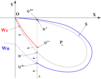
Figure 2. Sketch of the proof of Lemma 2.13, when $\boldsymbol{A^{+}}$ holds.

Now denote by $D^{u}(\tau)$ the bounded set enclosed by $\bar{W}^{u}(\tau)$, the segment between $\boldsymbol{Q^{u,-}}(\tau)$ and $\boldsymbol{H^{-}}(\tau)$ and the branch of $S(\tau)$ between $\boldsymbol{H^{-}}(\tau)$ and the origin: observe that by construction if $\boldsymbol{Q}\in D^{u}(\tau)$, then $\boldsymbol{y}(s,\tau,\boldsymbol{Q};2^{*})\in D^{u}(s)$ for any $s\leq\tau$. Since $S(\tau)\subset D^{u}(\tau)$ we see that if $\boldsymbol{y}(s)$ corresponds to a S.G.S. with slow decay, then $\boldsymbol{y}(s)\in S(s)$ for any $s\in{\mathbb{R}}$.
Reasoning in the same way but reversing the direction of $s$ we see that if $\boldsymbol{A^{-}}$ holds then we can construct $\bar{W}^{s}(\tau)$ for any $\tau\in{\mathbb{R}}$. Denote by $D^{s}(\tau)$ the bounded set enclosed by $\bar{W}^{s}(\tau)$, the segment between $\boldsymbol{Q^{s,+}}(\tau)$ and $\boldsymbol{H^{+}}(\tau)$ and the branch of $S(\tau)$ between $\boldsymbol{H^{+}}(\tau)$ and the origin. Then if $\boldsymbol{y}(s)$ corresponds to a singular solution, then $\boldsymbol{y}(s)\in S(s)$ for any $s\in{\mathbb{R}}$. So Lemma 2.13 follows. ∎

Now we give a Lemma which is useful to detect the $\omega$-limit set of solutions of (1.1)–(1.2) in the case where $\phi$ is a radial upper or lower solution of (1.8).

2.15 Lemma.

Let $U(r)$ and $V(r)$ be positive solutions of (1.8) either regular or singular and assume that there is $Z>0$ such that $U(Z)=V(Z)$ and $U^{\prime}(Z)<V^{\prime}(Z)$. Denote by

(2.19) $$\zeta(r)=\left\{\begin{array}[]{cc}V(r)&\textrm{if $r\leq Z$}\\ U(r)&\textrm{if $r\geq Z$}\end{array}\right.\,,\qquad\psi(r)=\left\{\begin{array}[]{cc}U(r)&\textrm{if $r\leq Z$}\\ V(r)&\textrm{if $r\geq Z$}\end{array}\right.$$

Assume $\boldsymbol{A^{-}},\boldsymbol{Gu},\boldsymbol{Gs}$ with $l_{u}\geq 2^{*}$ and $l_{s}\in[2^{*},\sigma^{*})$.

Then (1.8) admits no solutions $\phi(r)$ either regular or singular such that $0<\phi(r)\leq\zeta(r)$ and no solutions $\phi(r)$ such that $\phi(r)\geq\psi(r)$ for any $r>0$.

Proof.

From Proposition 2.12 we know that all the positive solutions have slow decay. Assume first $l_{s}\in[2^{*},\sigma^{*})$. Then from Remark 2.10 all the slow decay solutions of (1.8) cross each other indefinitely as $r\to+\infty$, so the Lemma easily follows. ∎

Reasoning in the same way we get the following:

2.16 Lemma.

Let $U(r)$, $V(r)$, $\zeta(r)$ and $\psi(r)$ be as in Lemma 2.15. Assume $\boldsymbol{A^{+}},\boldsymbol{Gu},\boldsymbol{Gs}$ with $l_{u}\in(\sigma_{*},2^{*}]$ and $l_{s}\in(2_{*};2^{*}]$.

Then (1.8) admits no solutions $\phi(r)$ either regular or singular such that $0<\phi(r)\leq\zeta(r)$ and no solutions $\phi(r)$ such that $\phi(r)\geq\psi(r)$ for any $r>0$.

3. Local existence

In this section we introduce some basic facts and definitions related to the problem (1.1)–(1.2), and exploiting techniques similar to those used in [27, §1, §2] (see also [22, Ch. II]), we prove local existence for the solutions of problem (1.1)–(1.2). For the remainder of this section we will make the following assumptions, in addition to $\mathbf{F0}$, on the potential $f$ in (1.1), i.e.:

• $\boldsymbol{Gu}$ holds and there is $D>0$ such that $\frac{\partial}{\partial y_{1}}[g(y_{1},s;l_{u})]\leq D|y_{1}|^{\delta}$ for any $0\leq y_{1}\leq 1$, and $0<s\leq 1$.
  

• There are $\ell\geq 0$, $\bar{C}>0$, $\delta>0$, $\varepsilon>0$ such that $|f(u,r)-f(u+h,r)|\leq\bar{C}hu^{\delta}r^{\ell}$ whenever $r\geq 1$, $0\leq u\leq 1$, and $0\leq h\leq\varepsilon$.

Assumption $\boldsymbol{Fu}$ is very close to $\boldsymbol{Gu}$ (and it is actually satisfied in all the motivating examples given in the introduction), while $\boldsymbol{Fs}$ is more standard and it is adapted from [27]. Let us introduce the following map

(3.1) $$w(x)=\left\{\begin{array}[]{ll}|x|^{\nu}&\textrm{ if $|x|\leq 1$}\\ |x|^{\ell/\delta}&\textrm{ if $|x|\geq 1$}\end{array}\right.\textrm{ where }0\leq\nu<m(l_{u}).$$

We emphasize that if $\ell=0$ then $w(x)\equiv 1$ for $|x|\geq 1$. Moreover if we set $\nu=0$ then $w(x)\equiv 1$ for $|x|\leq 1$ so we are dealing with bounded solutions, while if we set $\nu>0$ we can deal with solutions which are unbounded for $|x|$ small and are not defined for $x=0$.

Let us recall the definitions of continuous weak solution and $C_{B}$-mild solution to the problem (1.1)–(1.2).

3.1 Definition.

We say that a function $u$ is a continuous weak (c.w.) solution of (1.1)–(1.2) if $u$ is continuous and it is a distributional solution: i.e. if $u(x,0)=\phi(x)$ and, for any $\eta\in C^{2,1}({\mathbb{R}}^{n}\times[0,T])$ with $\eta\geq 0$ and $\mathop{\mathrm{missing}}{supp}\nolimits\eta(\cdot,t)\Subset{\mathbb{R}}^{n}$ for all $t\in[0,T]$, it holds true that

(3.2) $$\int_{{\mathbb{R}}^{n}}\!u(x,s)\eta(x,s)dx|_{0}^{T_{1}}\!=\!\int_{0}^{T_{1}}\!\!\int_{{\mathbb{R}}^{n}}\!\!\Big{[}u(x,s)\big{(}\eta_{t}+\Delta\eta\big{)}(x,s)+f(u,|x|)\eta(x,s)\Big{]}dxds$$

if $T_{1}\in[0,T]$. Further, u is a c.w. lower (respectively upper) solution of (1.1)–(1.2) if $u(x,0)\geq\phi(x)$ (resp. $u(x,0)\leq\phi(x)$) and we replace $``="$ in (3.2) by $``\geq"$ (resp. by $``\leq"$). We call a function $u$ a classical solution if it satisfies (1.1)–(1.2) and $u\in C^{2,1}({\mathbb{R}}^{n}\times(0,T))\cap C({\mathbb{R}}^{n}\times[0,T])$.

Let $\phi\in C_{B}({\mathbb{R}}^{n}):=C({\mathbb{R}}^{n})\cap L^{\infty}({\mathbb{R}}^{n})$. We introduce the following operators

(3.3) $$\begin{split}&e^{t\Delta}\phi:=(4\pi t)^{-n/2}\int_{{\mathbb{R}}^{n}}\exp\Big{(}-\frac{|x-y|^{2}}{4t}\Big{)}\phi(y)dy.\\ &F_{\phi}(u)=\Big{(}e^{t\Delta}\phi+\int_{0}^{t}e^{(t-s)\Delta}f(u(\cdot,s),|\cdot|)ds\Big{)}(x)\end{split}$$

3.2 Definition.

We say that u is a $C_{B}$-mild solution of (1.1)–(1.2) on ${\mathbb{R}}^{n}\times[0,T)$ if

(3.4) $$u\in C_{B}({\mathbb{R}}^{n}\times[0,T^{\prime}]):=C({\mathbb{R}}^{n}\times[0,T^{\prime}])\cap L^{\infty}({\mathbb{R}}^{n}\times[0,T^{\prime}]),\,\,0<T^{\prime}<T,$$

(3.5) $$u(x,t)=F_{\phi}(u(x,t)),\,\textrm{for}\,(x,t)\in{\mathbb{R}}^{n}\times[0,T).$$

Also, we say that $u$ is a $C_{B}$-mild lower solution (or upper) solution if $``="$ in (3.5) is replaced by $``\geq"$ ($``\leq"$ respectively).

We also consider the norm $\|\phi\|_{X}:=\|\phi w\|_{L^{\infty}({\mathbb{R}}^{n})}$ and the weighted space $X=L^{\infty}_{w}({\mathbb{R}}^{n})=\{\phi\mid\|\phi\|_{X}<+\infty\}$ where $w$ is defined in (3.1). We denote by $C_{S}({\mathbb{R}}^{n}\times[0,T^{\prime}]):=C(({\mathbb{R}}^{n}\backslash\ \{0\})\times[0,T^{\prime}])\cap L^{\infty}([0,T^{\prime}],X)$ and we give the following definiton

3.3 Definition.

We say that $u$ is a $C_{S}$-mild solution to (1.1)–(1.2) on $({\mathbb{R}}^{n}\backslash\ \{0\})\times[0,T)$ if $u\in C_{S}({\mathbb{R}}^{n}\times[0,T^{\prime}])$ for any $0<T^{\prime}<T$ and satisfies $u(x,t)=F_{\phi}(u(x,t))$ for $(x,t)\in({\mathbb{R}}^{n}\backslash\ \{0\})\times[0,T)$.

Note that if $\nu>0$ and $u$ is a $C_{S}$-mild solution then it may be unbounded as $x\to 0$. Therefore we can deal with initial data and solution having a singularity in the origin, and we will prove local existence and uniqueness for such initial data. It is worth recalling that with our assumptions we have singular stationary solutions $\phi_{S}$ which behave like $|x|^{-m(l_{u})}$ as $x\to 0$.

An interesting question, still open even for the starting case $f(u)=u^{q-1}$, is whether stationary S.G.S. are stable or not. One of the difficulties is in fact to prove local existence and uniqueness for nearby initial data (which is in general violated but maybe recovered in some special space and for some parameters, see [25]). In fact we cannot even hope for a general local uniqueness result: We need to prescribe a class of function within local uniqueness is recovered, due to the presence of self-similar solutions converging to singular data (see, e.g. [26, 22]), and to a new class of solutions with moving singularity recently described in [23, 24].

We stress that here we are forced to stay below $\phi_{S}$ since we need to require $\nu<m(l_{u})$, so we cannot start a stability analysis for stationary singular solutions.

The following result is a direct consequence of [27, Lemma 1.5].

3.4 Lemma.

Assume $\boldsymbol{Fu}$, $\boldsymbol{Fs}$. Let $u$ be a continuous weak upper (lower) solution of (1.1)–(1.2) with $n\geq 3$. Assume that there exist $k,\beta>0$, and $0<\alpha<2$ such that $f(u,x)<k\exp(\beta|x|^{\alpha}{})$ on ${\mathbb{R}}^{n}\times[0,T]$. Then $u(x,t)\geq(\leq)F_{\phi}(u(x,t))$ on ${\mathbb{R}}^{n}\times[0,T]$.

3.5 Remark.

By this lemma it follows that a c.w. solution of (1.1)–(1.2) satisfying either (3.4) in Definition 3.2 or the analogous weighted condition in Definition 3.3 is also respectively either a $C_{B}$-mild solution or a $C_{S}$ solution. The converse is also true (see the proof of [27, Lemma1.5]).

To prove Lemma 3.4 it is sufficient to adapt the proof of [27, Lemma 1.5] to the present case. By Lemma 3.4 we also have the next result.

3.6 Proposition.

Assume $\boldsymbol{Fu}$, $\boldsymbol{Fs}$. Suppose that $u$ is a continuous weak upper (resp. lower) solution of (1.7) in ${\mathbb{R}}^{n}\backslash\{0\}$ such that $\|u\|_{X}$ is bounded, then $u$ is a $C_{S}$-mild upper (resp. lower) solution of (1.1)–(1.2). The converse is also true, provided $\phi(x)\geq u(x,0)$ (resp. $\phi(x)\leq u(x,0)$). In particular if we set $\nu=0$ we see that a continuous bounded weak upper (resp. lower) solution of (1.7) is a $C_{B}$-mild solution of (1.1)–(1.2) and viceversa

Take $\rho>0$ and $\phi\in X$, and denote by $B_{\rho}:=B_{\rho}^{T}(0)\subseteq L^{\infty}([0,T];X)$ the ball of center $0$ and radius $\rho$, in $X$; the radius $\rho$ will be chosen properly later. We now prove local existence and uniqueness for $C_{B}$ and $C_{S}$-mild solutions.

3.7 Lemma.

Assume $\boldsymbol{Fu}$, $\boldsymbol{Fs}$. If the initial datum $\phi\in X$, there is $T_{\phi}>0$ such that the operator $F_{\phi}(u)$ defined by (3.3) has a unique fixed point in $B_{\rho}^{T}(\phi)$ for any $0<T<T_{\phi}$, and if $T_{\phi}<+\infty$, then $\lim_{t\to T^{-}_{\phi}}\|u(\cdot,t)\|_{X}=+\infty$.

Proof.

We claim that the operator $F_{\phi}$ maps $B_{\rho}$ in itself and it is a contraction: Then the Banach fixed point theorem provides existence and uniqueness of a fixed point $u$ for $F_{\phi}$.

Observe first that if $u\in B_{\rho}$, then $|u(x,t;\phi)|\leq\rho w(x)^{-1}$ a.e. in ${\mathbb{R}}^{n}\times[0,T]$. Here, we take $\rho=2(2D_{1}+2^{\nu+1}+2^{\ell/\delta})\|\phi\|_{X}$, where $D_{1}:=\textrm{e}^{-\nu/2}(16\nu)^{\nu/2}$.

From relation $\boldsymbol{Fu}$, for $|x|\leq 1$, we get

(3.6) $$\begin{aligned} f(u,|x|)&\leq f(\rho\omega^{-1}(x),|x|)\leq g(\rho|x|^{m(l_{u})-\nu},\ln(|x|);l_{u})|x|^{-(2+m(l_{u}))}\\ &\leq k^{-}|x|^{\delta(m(l_{u})-\nu)-2-\nu},\end{aligned}$$

where $$k^{-}=D\rho^{1+\delta} v\in B_{\rho}$$. Then, for any , we also have

(3.7) $$\begin{aligned} |f(&u,|x|)-f(v,|x|)|=\left|\int_{0}^{1}\frac{\partial f}{\partial u}(su+(1-s)v),|x|)[u-v]ds\right|\\ &\leq\frac{\partial g}{\partial y_{1}}\big{(}\rho|x|^{m(l_{u})-\nu},\ln(|x|);l_{u}\big{)}|x|^{-(2+m(l_{u}))}|(u-v)(x)|\,|x|^{m(l_{u})}\\ &\leq\frac{\partial g}{\partial y_{1}}\big{(}\rho|x|^{m(l_{u})-\nu},\ln(|x|);l_{u}\big{)}|x|^{-(2+m(l_{u}))}\|(u-v)(x)|\,|x|^{\nu}\|_{\infty}\\ &\leq k^{-}|x|^{\delta(m(l_{u})-\nu)-2-\nu}\|u-v\|_{X},\end{aligned}$$

where we have redefined $k^{-}=D\max\{\rho^{1+\delta},\rho^{\delta}\}$. From $\boldsymbol{Fs}$, for $|x|\geq 1$, we also get

(3.8) $$\begin{aligned} f(u,|x|)=f(u,|x|)-f(0,|x|)\leq\bar{C}|u|^{1+\delta}|x|^{\ell}\leq\bar{C}\rho^{1+\delta}|x|^{-\ell/\delta}\leq k^{+}w(x)^{-1},\end{aligned}$$

(3.9) $$\begin{aligned} |f(u,|x|)-f(v,|x|)|&\leq|u|^{\delta}|v-u||x|^{\ell}\leq\bar{C}\frac{\rho^{\delta}}{|x|^{\ell}}\|u-v\|_{\infty}|x|^{\ell}\\ &\leq k^{+}w(x)^{-1}\|u-v\|_{X},\\ \end{aligned}$$

with $k^{+}\!=\!\bar{C}\max\{\rho^{1+\delta},\rho^{\delta}\}$. Till the end of the proof we need the following straightforward estimate: Let $A\in(0,n)$ and denote by $\Gamma$ the Euler Gamma function, then:

(3.10) $$\int_{{\mathbb{R}}^{n}}\frac{\textrm{e}^{-\frac{|\eta|^{2}}{4}}}{\big{(}4\pi\big{)}^{n/2}|\eta|^{A}}d\eta\leq\frac{1}{2^{n-1}(n-A)\Gamma(n/2)}+\int_{|\eta|\geq 1}\textrm{e}^{-\frac{|\eta|^{2}}{4}}d\eta\leq C(A)\,,$$

and we can set $C(A)=2$ if $A\in(0,n-1)$. We now proceed to prove that $F_{\phi}\colon B_{\rho}\to B_{\rho}$. From (3.3) we have that

(3.11) $$|F_{\phi}(u)|(x,t) \leq|e^{t\Delta}\phi|(x)+\int_{0}^{t}\int_{{\mathbb{R}}^{n}}\frac{\exp\Big{(}-\frac{|x-y|^{2}}{4(t-s)}\Big{)}}{\big{(}4\pi(t-s)\big{)}^{n/2}}f(u(y,s),|y|)dyds$$

$$\leq w^{-1}(x)\|e^{t\Delta}\phi\|_{X}(t)+w^{-1}(x)I,$$

where

$$I=w(x)\int_{0}^{t}\bigg{(}\int_{|y|\leq 1}+\int_{|y|\geq 1}\bigg{)}\frac{\exp\Big{(}-\frac{|x-y|^{2}}{4s}\Big{)}}{\big{(}4\pi s\big{)}^{n/2}}f\big{(}u,|y|\big{)}dyds=:I_{a}+I_{b}.$$

Using (3.6)-(3.7) we get the following

(3.12) $$I_{a} \leq k^{-}\int_{0}^{t}\bigg{(}\int_{\frac{|x|}{2}\leq|y|\leq 1}+\int_{|y|\leq\frac{|x|}{2}}\bigg{)}\frac{w(x)\exp\Big{(}-\frac{|x-y|^{2}}{4s}\Big{)}}{\big{(}4\pi s\big{)}^{n/2}|y|^{2-\delta(m(l_{u})-\nu)+\nu}}dyds$$

$$=:k^{-}(I_{a}^{-}+I_{a}^{+})$$

and

$$I_{a}^{-} \leq 2^{\nu}\int_{0}^{t}\int_{\frac{|x|}{2}\leq|y|\leq 1}\frac{\exp\Big{(}-\frac{|x-y|^{2}}{4s}\Big{)}}{\big{(}4\pi s\big{)}^{n/2}|y|^{2-\delta(m(l_{u})-\nu)}}dyds$$

$$\leq 2^{\nu}\int_{0}^{t}\int_{{\mathbb{R}}^{n}}\frac{\exp\Big{(}-\frac{|y|^{2}}{4s}\Big{)}}{\big{(}4\pi s\big{)}^{n/2}|y|^{2-\delta(m(l_{u})-\nu)}}dyds$$

$$\leq 2^{\nu}\int_{0}^{t}\int_{{\mathbb{R}}^{n}}\frac{\exp(-|\eta|^{2})|\eta|^{\delta(m(l_{u})-\nu)-2}}{(\pi)^{n/2}s^{1-\delta(m(l_{u})-\nu)/2}}d\eta ds\leq K^{-}t^{\delta(m(l_{u})-\nu)/2},$$

where $K^{-}>0$ is a positive constant, and we used the fact that the convolution of radial decreasing function is radial decreasing too (see [27, Lemma 1.4]), and that $n-3+\delta(m(l_{u})-\nu)>-1$.

Since $|x-y|\geq\big{|}|x|-|y|\big{|}$ we get

$$\,\,\,I_{a}^{+} \leq\int_{0}^{t}\int_{|y|\leq\frac{|x|}{2}}\frac{w(x)\exp\Big{(}-\frac{|x|^{2}}{16s}\Big{)}}{\big{(}4\pi s\big{)}^{n/2}|y|^{2+\nu-\delta(m(l_{u})-\nu)}}dyds$$

$$\leq\int_{0}^{t}\int_{|y|\leq\frac{|x|}{2}}\frac{w(x)\exp\Big{(}-\frac{|x|^{2}}{32s}\Big{)}\exp\Big{(}-\frac{|y|^{2}}{8s}\Big{)}}{\big{(}4\pi s\big{)}^{n/2}|y|^{2+\nu-\delta(m(l_{u})-\nu)}}dyds$$

$$\leq\int_{0}^{t}\frac{w(x)\exp\Big{(}-\frac{|x|^{2}}{32s}\Big{)}}{s^{1-[\delta(m(l_{u})-\nu)/2]+\nu/2}}ds\int_{{\mathbb{R}}^{n}}\frac{\exp\Big{(}-\frac{|\eta|^{2}}{8}\Big{)}}{\big{(}4\pi\big{)}^{n/2}|\eta|^{2+\nu-\delta(m(l_{u})-\nu)}}d\eta$$

$$\leq 2^{n/2}C\int_{0}^{t}\frac{w(x)}{s^{1-\delta m(l_{u})/2+\nu/2}}\exp\Big{(}-\frac{|x|^{2}}{32s}\Big{)}ds$$

where we used that $2+\nu-\delta(m(l_{u})-\nu)<2+m(l_{u})<n$, and $C=C(2+m(l_{u}))$ is the constant defined in (3.10). Now we need to distinguish between the $|x|\leq 1$ and the $|x|\geq 1$ case. Assume the former so that $w(x)=|x|^{\nu}$, and observe that $h(a):=\textrm{e}^{-a/32}a^{\nu/2}\leq D_{1}=h(16\nu)$; for any $a\geq 0$ we get

(3.13) $$I_{a}^{+}\leq D_{1}C\int_{0}^{t}\frac{1}{s^{1-[\delta(m(l_{u})-\nu)/2]}}ds\leq K^{+}t^{[\delta(m(l_{u})-\nu)/2]}.$$

where $K^{+}=\frac{D_{1}C}{\delta(m(l_{u})-\nu)/2}>0$ is a constant. When $|x|\geq 1$ so that $w(x)=|x|^{\ell/\delta}$; setting $\bar{h}(a):=\textrm{e}^{-a/64}a^{\ell/2\delta}$ we find $\bar{h}(a)\leq D_{2}:=\bar{h}(32\ell/\delta)$ for any $a\geq 0$ and similarly $\tilde{h}(a):=\textrm{e}^{-a/64}a^{1-[\delta(m(l_{u})-\nu-1/\ell)/2]+\nu/2}$ is bounded, say $\tilde{h}(a)\leq D_{3}$. Thus

(3.14) $$I_{a}^{+} \leq C\int_{0}^{t}\left[\left(\frac{|x|^{2}}{s}\right)^{\frac{\ell}{2\delta}}\exp\Big{(}-\frac{|x|^{2}}{64s}\Big{)}\right]\frac{\exp\Big{(}-\frac{1}{64s}\Big{)}}{s^{1-[\delta(m(l_{u})-\nu-1/\ell)/2]+\nu/2}}ds$$

$$\leq CD_{2}\int_{0}^{t}\bar{h}(\frac{|x|^{2}}{s})\tilde{h}(\frac{1}{s})ds\leq CD_{2}D_{3}t\leq\,K^{+}t$$

with a possibly larger constant $K^{+}$. Now we estimate $I_{b}$. From (3.8)–(3.9) we get:

(3.15) $$I_{b}\leq k^{+}w(x)\int_{0}^{t}\bigg{(}\int_{|y|\geq\max\{\frac{|x|}{2},1\}}+\int_{1\leq|y|\leq\frac{|x|}{2}}\bigg{)}\frac{\exp\Big{(}-\frac{|x-y|^{2}}{4s}\Big{)}}{\big{(}4\pi s\big{)}^{n/2}|y|^{\ell/\delta}}dyds$$

$$=:k^{+}(I_{b}^{-}+I_{b}^{+})\,.$$

Observing that $\hat{h}(a)=a^{\ell/(2\delta)}\textrm{e}^{-a/32}\leq\hat{h}(8\ell/\delta)$ and $C_{b}=2^{3n/2}\hat{h}(8\ell/\delta)$, we find

$$I_{b}^{-}\leq w(x)\int_{0}^{t}\int_{|y|\geq\max\{\frac{|x|}{2},1\}}\frac{\exp\Big{(}-\frac{|x-y|^{2}}{4s}\Big{)}}{\big{(}4\pi s\big{)}^{n/2}|y|^{\ell/\delta}}dyds\leq\int_{0}^{t}\frac{w(x)}{w(\max\{\frac{|x|}{2},1\})}\leq 2^{\ell/\delta}t,$$

$$\begin{aligned} I_{b}^{+}&\leq\int_{0}^{t}w(x)\textrm{e}^{-\frac{|x|^{2}}{32s}}ds\int_{1\leq|y|\leq\frac{|x|}{2}}\frac{\textrm{e}^{-\frac{|x|^{2}}{32s}}}{\big{(}4\pi s\big{)}^{n/2}}dy\leq 2^{3n/2}|x|^{\ell/\delta}t\textrm{e}^{-\frac{|x|^{2}}{32t}}\leq C_{b}t^{1+\frac{\ell}{2\delta}},\end{aligned}$$

Therefore, there is $K>0$ such that $I\leq K\max\{t^{1+\ell/(2\delta)},t,t^{\delta(m(l_{u})-\nu)/2}\}$, with $K=K(n,\ell,\nu,\|\phi\|_{X})$ and relation (3.11) reduces to

(3.16) $$|F_{\phi}(u)|(x,t)\leq w^{-1}(x)\|e^{t\Delta}\phi\|_{X}\!+w^{-1}(x)K\max\{T^{1+\ell/(2\delta)},T,T^{\delta(m(l_{u})-\nu)/2}\}.\!\!\!$$

To estimate the term $w^{-1}(x)\|e^{\Delta t}\phi\|_{X}$ we follow an approach similar to the one used above. Indeed, we rewrite $e^{t\Delta}\phi(x)$ as follows

(3.17) $$e^{t\Delta}\phi(x)=\bigg{(}\int_{|y|\leq 1}\!\!+\int_{|y|\geq 1}\!\!\bigg{)}\frac{\exp\Big{(}-\frac{|x-y|^{2}}{4t}\Big{)}}{\big{(}4\pi t\big{)}^{n/2}}\phi(y)dy=:I_{\alpha}+I_{\beta}.$$

Hence, we get

$$I_{\alpha} \leq\|\phi\|_{X}\bigg{(}\int_{\frac{|x|}{2}\leq|y|\leq 1}+\int_{|y|\leq\min\{\frac{|x|}{2},1\}}\bigg{)}\frac{\exp\Big{(}-\frac{|x-y|^{2}}{4t}\Big{)}}{\big{(}4\pi t\big{)}^{n/2}w(y)}dy=:I_{\alpha}^{-}+I_{\alpha}^{+}.$$

For $\frac{|x|}{2}\leq|y|\leq 1$, we reach

(3.18) $$I_{\alpha}^{-} \leq\frac{\|\phi\|_{X}2^{\nu}}{w(x)}\int_{\frac{|x|}{2}\leq|y|\leq 1}\frac{\exp\Big{(}-\frac{|x-y|^{2}}{4t}\Big{)}}{\big{(}4\pi t\big{)}^{n/2}}dy$$

$$\leq\frac{\|\phi\|_{X}}{w(x)}2^{\nu}\int_{{\mathbb{R}}^{n}}\frac{\exp\Big{(}-\frac{|y|^{2}}{4t}\Big{)}}{\big{(}4\pi t\big{)}^{n/2}}dy=\frac{\|\phi\|_{X}2^{\nu}}{w(x)}.$$

For the term $I_{\alpha}^{+}$, using (3.10) we obtain

$$I_{\alpha}^{+} \leq\|\phi\|_{X}\exp\Big{(}\frac{-|x|^{2}}{32t}\Big{)}\int_{|y|\leq\min\{\frac{|x|}{2},1\}}\frac{\exp\Big{(}-\frac{|y|^{2}}{8t}\Big{)}}{\big{(}4\pi t\big{)}^{n/2}|y|^{\nu}}dy$$

$$\leq\|\phi\|_{X}\exp\Big{(}\frac{-|x|^{2}}{32t}\Big{)}\int_{{\mathbb{R}}^{n}}\!\!\!\frac{\exp\Big{(}-\frac{|\eta|^{2}}{4}\Big{)}}{\big{(}4\pi\big{)}^{n/2}|\eta|^{\nu}t^{\nu/2}}d\eta\leq 2\|\phi\|_{X}\frac{\exp\Big{(}\frac{-|x|^{2}}{32t}\Big{)}}{t^{\nu/2}}.\!\!\!\!\!$$

Now, arguing as in (3.13), (3.14) we find for $|x|\leq 1$

(3.19) $$I_{\alpha}^{+} \leq 2\|\phi\|_{X}\frac{\Big{(}\frac{|x|^{2}}{t}\Big{)}^{\nu/2}\exp\Big{(}\frac{-|x|^{2}}{32t}\Big{)}}{|x|^{\nu}}\leq\frac{2D_{1}\|\phi\|_{X}}{w(x)}$$

while for $|x|\geq 1$, since $\bar{h}(a)=a^{\ell/(2\delta)}\textrm{e}^{-a/64}\leq D_{2}$, we get

$$I_{\alpha}^{+} \leq 2\|\phi\|_{X}\frac{\Big{(}\frac{|x|^{2}}{t}\Big{)}^{\ell/(2\delta)}\exp\Big{(}\frac{-|x|^{2}}{64t}\Big{)}}{w(x)}\;\frac{\exp\Big{(}\frac{-|x|^{2}}{64t}\Big{)}}{t^{\nu/2-\ell/(2\delta)}}\leq\varepsilon(t)\;\frac{2D_{2}\|\phi\|_{X}}{w(x)}$$

where $\varepsilon(t):=\exp\big{(}\frac{-1}{64t}\big{)}t^{\ell/(2\delta)-nu/2}\to 0$ as $t\to 0$. So choosing $t$ small enough we can assume that (3.19) holds for $|x|\geq 1$, too. Take into account $I_{\beta}$, to get

(3.20) $$\begin{split}I_{\beta}&\leq\frac{\|\phi\|_{X}}{w(x/2)}\int_{|y|\geq\frac{|x|}{2}}\frac{\exp\Big{(}-\frac{|x-y|^{2}}{4t}\Big{)}}{\big{(}4\pi t\big{)}^{n/2}}\\ &\leq\frac{\|\phi\|_{X}}{w(x/2)}\|\phi\|_{X}\int_{{\mathbb{R}}^{n}}\frac{\exp\Big{(}-\frac{|\eta|^{2}}{4}\Big{)}}{\big{(}4\pi\big{)}^{n/2}}d\eta\\ &\leq\frac{\|\phi\|_{X}}{w(x/2)}\leq\frac{\|\phi\|_{X}}{w(x)}\max\{2^{\nu},2^{\ell/\delta}\}\end{split}$$

Collecting the estimates (3.17)-(3.18)-(3.19)-(3.20), we have that relation (3.16), and hence (3.11), for $T\leq 1$ gives

$$\|F_{\phi}(u)\|_{X}(T) \leq\big{(}2D_{1}+2^{\nu+1}+2^{\ell/\delta}\big{)}\|\phi\|_{X}+K\max\{T,T^{\delta(m(l_{u})-\nu)/2}\}$$

$$\leq\rho/2+CT\|\phi\|_{X}+K\max\{T,T^{\delta(m(l_{u})-\nu)/2}\}.$$

Let $T_{0}=T_{0}(n,\ell,\|\phi\|_{X},\nu,\rho)>0$ be such that, for any $T\leq T_{0}$,

$$K\max\{T,T^{\delta(m(l_{u})-\nu)/2}\}<\rho/2.$$

Then, we have that

$$\|F_{\phi}(u)\|_{L^{\infty}(0,T;X)}\leq\rho,\textrm{ for any }T\leq T_{0}$$

and hence $F_{\phi}$ maps $B_{\rho}$ into $B_{\rho}$, for $T\leq T_{0}$.

Analogously, let $u,v\in B_{\rho}$, we get

(3.21) $$\begin{split}|F_{\phi}(u)-F_{\phi}(v)|(x,t)\leq&\int_{0}^{t}\Big{(}\int_{|y|\leq 1}\frac{k^{-}\exp\Big{(}-\frac{|x-y|^{2}}{4s}\Big{)}}{\big{(}4\pi s\big{)}^{n/2}|y|^{2+\nu-\delta(m(l_{u})-\nu)}}dy+\\ &+\int_{|y|\geq 1}\frac{k^{+}\exp\Big{(}-\frac{|x-y|^{2}}{4s}\Big{)}}{\big{(}4\pi s\big{)}^{n/2}|y|^{\ell/\sigma}}dy\Big{)}\|u-v\|_{X}ds.\end{split}$$

Repeating the argument of (3.12) and (3.13) we get

(3.22) $$\|[F_{\phi}(u)-F_{\phi}(v)]\|_{X}(t)\leq k^{-}[K^{-}t^{\delta(m(l_{u})-\nu)/2}+K^{+}t]+k^{+}[2^{\ell/\delta}+C_{b}t^{\ell/(2\delta)}]t.$$

Therefore, taking $T<T_{0}$ sufficiently small, it follows that $F_{\phi}$ maps $B_{\rho}$ into $B_{\rho}$ and it is actually a contraction. From the contraction principle, we obtain existence and uniqueness of a fixed point $u$ in $B_{\rho}$ which in turn implies the existence and local uniqueness of a $C_{B}$-mild solution to (1.1)–(1.2). Then, we can restart the reasoning, by setting $\phi(x)=u(x,T)$ and go up to $T_{\phi}$ by a ladder argument. Note that if $T_{\phi}<\infty$ and $\lim_{t\to T_{\phi}}\|u(x,t)\|_{X}$ is bounded we can restart the ladder argument and obtain a continuation interval $[0,T^{\prime}]\supset[0,T_{\phi})$ and this is a contradiction. Hence if $T_{\phi}<\infty$ we get $\lim_{t\to T_{\phi}}\|u(x,t)\|_{X}=+\infty$. ∎

As a direct consequence of Lemma 3.7 we have the following existence result

3.8 Theorem.

Assume $\boldsymbol{Fu}$, $\boldsymbol{Fs}$. Let $\phi\in X$ be the initial datum for the Equation (1.1). Then problem (1.1)–(1.2) has a unique weak solution $u$ on ${\mathbb{R}}^{n}\times[0,T_{\phi})$, $T_{\phi}>0$. If $\phi\in C_{B}({\mathbb{R}}^{n})=C({\mathbb{R}}^{n})\cap L^{\infty}({\mathbb{R}}^{n})$ then $u\in C\big{(}{\mathbb{R}}^{n}\times[0,T_{\phi})\big{)}\cap L^{\infty}\big{(}{\mathbb{R}}^{n}\times[0,T_{\phi})\big{)}$, and if $T_{\phi}<+\infty$ then $\lim_{t\to T_{\phi}^{-}}\|u(\cdot,t)\|_{L^{\infty}({\mathbb{R}}^{n})}=+\infty$. Similarly, if $\phi\in C_{S}({\mathbb{R}}^{n})=C({\mathbb{R}}^{n}\backslash\{0\})\cap L^{\infty}_{w}({\mathbb{R}}^{n})$ then $u\in C\big{(}({\mathbb{R}}^{n}\backslash\{0\})\times[0,T_{\phi})\big{)}\cap L^{\infty}([0,T_{\phi}),L^{\infty}_{w}({\mathbb{R}}^{n}))$, and if $T_{\phi}<+\infty$, then $\lim_{t\to T_{\phi}^{-}}\|u(\cdot,t)w(\cdot)\|_{L^{\infty}({\mathbb{R}}^{n})}=+\infty$.

Furthermore, if $\phi\geq 0$, then $u\geq 0$; if $\phi$ is radial, then $u$ is radial in $x$; if $\phi$ is radial and radially non-increasing, then $u$ is non-increasing in $|x|$.

3.9 Remark.

Assume that $f$ is locally Hölder continuous in $x$ and assume also there exists $l\geq 0$ such that $f(u,|x|)|x|^{-l}=f(u,r)r^{-l}$ is locally Lipschitz in $u$ uniformly with respect to $x$ (and so in $r$) in any bounded subset of ${\mathbb{R}}^{n}$. In such a case, using [27, Lemma 1.2] and arguing as in [27], one can verify that the $C_{B}$-solutions are actually classical.

In particular, we have that the potentials in (1.3)–(1.5) verify these conditions.

As a consequence of Proposition 3.6 and Lemma 3.7 we have the following result

3.10 Theorem.

Assume that $\boldsymbol{Fu}$, $\boldsymbol{Fs}$ are verified. Then

• Suppose that $\bar{u}$ and $\underline{u}$ are $C_{S}$-mild upper and lower solutions of (1.1)-(1.2) on ${\mathbb{R}}^{n}\times[0,T)$. Then $\bar{u}>\underline{u}$ on ${\mathbb{R}}^{n}\times[0,T)$, and the unique $C_{S}$-mild solution of (1.1)-(1.2) on ${\mathbb{R}}^{n}\times[0,T_{\phi})$ satisfies that $\underline{u}\leq u\leq\bar{u}$ on ${\mathbb{R}}^{n}\times[0,T)$ and $T_{\phi}>T$.
  

• If the initial value $\phi$ in (1.2) is a c.w. upper (lower) solution of (1.7), then the $C_{S}$-mild solution u of (1.1)-(1.2) is non-increasing (non-decreasing) in $t\in[0,T_{\phi})$.
  

• If $\phi$ is radial, then $\bar{u}$, $\underline{u}$ and $u$ are radial for any $t$ in their dominion of definition.
  

• If $\phi$ is a c.w. upper (lower) solution but not a solution of (1.7), then $u_{t}(x,t)<(>)0$, $t>0$.

The proof of this theorem is omitted because it can be easily derived by adapting that one of [27, Theorem 2.4] to the current case. We point out that claim (iv) follows directly by exploiting a comparison principle, arguing as in [27, Lemma 2.6] (see, e.g., [11] for a full-fledged proof of this well-established comparison argument. See also [14]). Further, a result analogous to Theorem 3.10 holds true also in the even simpler case of the $C_{B}$-mild solutions of (1.1)–(1.2) on ${\mathbb{R}}^{n}\times[0,T)$ (see [27, Theorem 2.4]).

To conclude this section we give a result about the global solution $u(x,t;\phi)$ of the problem (1.1)–(1.2), for $\phi\in C_{B}({\mathbb{R}}^{n})$ or $\phi\in C_{S}({\mathbb{R}}^{n})$.

3.11 Remark.

Assume that $\phi$ is a singular upper (respectively lower) solution. From Theorem 3.10 point (iv), which translates [27, Lemma 2.6] to the current case, it follows that $\lim_{t\to T_{\phi}}u(x,t;\phi)=u(x,T_{\phi};\phi)$ exists for any $x\neq 0$. Following the proof of Claim 2 of [27, Theorem 3.6], using Lebesgue dominated convergence theorem and regularity theory for elliptic equation we see that $u(x,T_{\phi};\phi)$ is a distributional solution of (1.7). Moreover if $\phi$ is radial then $u(x,T_{\phi};\phi)$ is radial too.

4. Long time behavior: main results

Now we are ready to state and prove our results in their general form, from which Theorems 1.5, 1.6, and Corollary 1.8 follow.

Let $w(x)$ be defined as in (3.1).

4.1 Theorem.

Assume $\boldsymbol{Fu}$, $\boldsymbol{Fs}$, $\boldsymbol{A^{-}}$, $\boldsymbol{Gu}$ and $\boldsymbol{Gs}$, with $2^{*}\leq l_{s}<\sigma^{*}$ and $l_{u}\geq 2^{*}$.

• If $\phi(x)\lneqq U(|x|,\alpha)$ for some $\alpha>0$, then it holds that $\|u(x,t;\phi)\|_{\infty}\to 0$ and $\|u(x,t;\phi)(1+|x|^{\nu})\|_{\infty}\to 0$ as $t\to+\infty$ for any $0\leq\nu<m(l_{s})$.
  

• Let $\phi$ be a continuous initial data or a singular one such that $\|\phi(x)w(x)\|_{\infty}$ is bounded, for some $\nu\in[0,m(l_{s}))$. If $\phi(x)\gneqq U(|x|,\alpha)$ for some $\alpha>0$, then $\|u(x,t;\phi)w(x)\|_{\infty}$ must blow up in finite time.

This result establishes that G.S. with s.d. are on the border between the basin of attraction of the null solutions and initial data which blow up in finite time, in the range of the considered parameters. We emphasize that we need $l_{s}<\sigma^{*}$, but $l_{u}$ has no upper bound: this allows e.g. $f(u,r)=(1+r^{a})u^{q}$ where $q>\sigma^{*}$ and $a\in\big{(}\frac{2}{\sigma^{*}-2}(q-\sigma^{*}),\frac{n-2}{2}(q-2^{*})\big{)}$. It is easy to check that $\boldsymbol{A^{-}}$ might be replaced by $\boldsymbol{H-}$, and that Theorem 4.1 implies Theorem 1.3.

Next, we state Theorems 4.2 and 4.3 from which Theorems 1.5, 1.6, and Corollary 1.8 follow. These results concern a wider range of parameters, and enable us to understand something about the border of the basin of attraction of the null solution and of infinity, i.e. blowing up solutions. We start from a generalization of a result by Wang in [27] concerning slow decay solutions.

4.2 Theorem.

Assume $\boldsymbol{Fu}$, $\boldsymbol{Fs}$, $\boldsymbol{Gu}$, $\boldsymbol{Gs}$. Assume either $\boldsymbol{A^{+}}$ with $l_{u},l_{s}\in(2_{*},2^{*}]$ or $\boldsymbol{A^{-}}$ with $l_{u}\geq 2^{*}$ and $2^{*}\leq l_{s}<\sigma^{*}$. Then there exists a one-parameter family of upper radial solutions of (1.7) denoted by $\chi_{\tau}(x)$, such that $u(x,t;\chi)$ converge to the null solution as $t\to+\infty$ and with the properties described in Theorem 1.5; in particular they have slow decay.

Such a result is proved in [27] for $f(u,r)=|x|^{\delta}u^{q-1}$, but as far as we are aware is new even for the potential considered in [1] and [28], i.e. even for $f$ as in (1.3) with $k(r)\neq r^{\delta}$ and $f$ as in (1.4) also when $k_{1}=k_{2}=1$. Theorem 4.2 seems to suggest that slow decay is the optimal decay rate to have solutions of (1.1) defined for any $t$. In fact we have the following result which is in contradiction with this idea (as far as we are aware these results are new even for the case $f(u)=u^{q-1}$).

4.3 Theorem.

Assume $\boldsymbol{Fu}$, $\boldsymbol{Fs}$, $\boldsymbol{Gu}$, $\boldsymbol{Gs}$. Assume either $\boldsymbol{A^{+}}$ with $l_{u},l_{s}\in(2_{*},2^{*}]$ or $\boldsymbol{A^{-}}$ with $l_{u},l_{s}\geq 2^{*}$. Then there are one-parameter families of upper and lower radial solution of (1.7), denoted by $\zeta_{\tau}(x)$ and $\psi_{\tau}(x)$ having the properties described in Theorem 1.6.

We stress that Remark 1.7 holds also in this case.
The relevance of Theorems 4.2 and 4.3 is more clear if we recall the comparison principle: if we choose any $\phi(x)$ even non radial, such that $\phi\leq\not\equiv\zeta_{\tau}$ for some $\tau$ then $u(x,t;\phi)$ converge to the null solution, while if $\phi\geq\not\equiv\psi_{\tau}(x)$ then $u(x,t;\phi)$ blows up in finite time. In fact Corollary 1.8 holds in this more general context too.

4.1. Construction of upper and lower-solutions for the stationary problem.

From now to the end we always assume $\boldsymbol{F0},\boldsymbol{Fu},\boldsymbol{Fs}$ (in order to guarantee local existence of solutions) without further mentioning. We introduce the following notation; we denote by $\boldsymbol{y^{u}}(s,\alpha;l_{u})$ the trajectory of (2.2) corresponding to the regular solution $U(r,\alpha)$ of (1.8), by $\boldsymbol{y^{u}}(s,\infty;l_{u})$ the trajectory corresponding to the singular solution $U(r,\infty)$, by $\boldsymbol{y^{s}}(s,\beta;l_{s})$ the trajectory corresponding to the fast decay solution $V(r,\beta)$, and by $\boldsymbol{y^{s}}(s,\infty;l_{s})$ the trajectory corresponding to the slow decay solution $V(r,\infty)$.

4.4 Lemma.

Fix $S\in{\mathbb{R}}$. Assume $l_{u}>2^{*}$, then $\boldsymbol{y^{u}}(s,\alpha;l_{u})$ converges to $\boldsymbol{y^{u}}(s,\infty;l_{u})$ as $\alpha\to+\infty$, uniformly for $s\leq S$.
Assume $2_{*}<l_{s}<2^{*}$, then $\boldsymbol{y^{s}}(s,\beta;l_{s})$ converges to $\boldsymbol{y^{s}}(s,\infty;l_{s})$, uniformly for $s\geq S$.

We think it is worth recalling that in the cases considered $U(r,\infty)$ and $V(r,\infty)$ are the unique singular and slow decay solutions of (1.8).

Proof of Lemma 4.4.

Assume $l_{u}>2^{*}$, fix $\tau\in{\mathbb{R}}$ and set $\boldsymbol{Q}(\alpha)=\boldsymbol{y^{u}}(\tau,\alpha;l_{u})$. We recall that $W^{u}(\tau;l_{u})$ is a path joining the origin and $\boldsymbol{R}=\boldsymbol{y^{u}}(\tau,+\infty;l_{u})$; moreover $\boldsymbol{Q}(\alpha)\to\boldsymbol{R}$ as $\alpha\to\infty$, see Remark 2.6 and [5]. If $I\subset{\mathbb{R}}$ is a compact interval, then $\boldsymbol{y^{u}}(t,\alpha;l_{u})\to\boldsymbol{y^{u}}(\tau,+\infty;l_{u})$ for any $t\in I$. But $\boldsymbol{y^{u}}(t,\alpha;l_{u})$ and $\boldsymbol{y^{u}}(\tau,+\infty;l_{u})$ are solutions of (2.2) hence $\boldsymbol{y^{u}}(t,\alpha;l_{u})$ is equibounded and equicontinuous for $\alpha$ large so we conclude using Ascoli theorem. The case $2_{*}<l_{s}<2^{*}$ is completely analogous. ∎

Analogously, using the fact that $\boldsymbol{y^{u}}(s,\alpha;l_{u})\to(0,0)$ as $s\to-\infty$, and $\boldsymbol{y^{s}}(s,\beta;l_{s})\to(0,0)$ as $s\to+\infty$ for any $\alpha>0$ $\beta>0$, we get the following

4.5 Lemma.

Assume $\boldsymbol{Gu}$ with $l_{u}>2_{*}$, and fix $S\in{\mathbb{R}}$; then the trajectory $\boldsymbol{y^{u}}(s,\alpha_{2};l_{u})$ converges to $\boldsymbol{y^{u}}(s,\alpha_{1};l_{u})$ as $\alpha_{2}\to\alpha_{1}$, uniformly for $s\leq S$.
Assume $\boldsymbol{Gs}$ with $l_{s}>2_{*}$, and fix $S\in{\mathbb{R}}$; then $\boldsymbol{y^{s}}(s,\beta_{2};l_{s})$ converges to $\boldsymbol{y^{s}}(s,\beta_{1};l_{s})$ as $\beta_{2}\to\beta_{1}$, uniformly for $s\geq S$.

From Lemmas 4.4 and 4.5 we easily get the following.

4.6 Lemma.

Let $\rho>0$ be arbitrarily small. Assume $\boldsymbol{Gu}$, $\boldsymbol{Gs}$ with $l_{u},l_{s}\geq 2^{*}$, and $\boldsymbol{A^{-}}$. Then for any $\alpha_{1}\geq 0$, $U(r,\alpha_{2})$ converges to $U(r,\alpha_{1})$ as $\alpha_{2}\to\alpha_{1}$, uniformly for $r\geq 0$. Further, assume $l_{u}>2^{*}$, then $U(r,\alpha_{2})$ converges to $U(r,\infty)$ as $\alpha_{2}\to+\infty$, uniformly for $r\geq\rho$.
Similarly assume $\boldsymbol{Gu}$, $\boldsymbol{Gs}$ with $l_{u},l_{s}\in(2_{*},2^{*}]$, and $\boldsymbol{A^{+}}$. Then for any $\beta_{1}\geq 0$, $V(r,\beta_{2})$ converges to $V(r,\beta_{1})$ as $\beta_{2}\to\beta_{1}$, uniformly for $r\geq\rho$. Moreover, if $2_{*}<l_{s}<2^{*}$ then we can take also $\beta_{1}=+\infty$.

Proof.

Assume $\boldsymbol{Gu}$, $\boldsymbol{Gs}$ with $l_{u},l_{s}\geq 2^{*}$, and $\boldsymbol{A^{-}}$ and choose $\alpha_{1}\in(0,+\infty)$. Then from Lemma 4.5 we easily see that $U(r,\alpha_{2})$ converges to $U(r,\alpha_{1})$ uniformly for $r$ in compact subsets of $r\in(0,\infty)$. However using Ascoli theorem and working directly on (1.8) we easily get uniform convergence for $r\in[0,\rho)$ too, see e.g. the Appendix of [9] for more details (in a much more general context); so we have uniform convergence in $[0,R]$. From Proposition 2.12 we know that $U(r,\alpha)$ is a G.S. with slow decay for any $\alpha>0$, hence $y^{u}_{1}(s,\alpha;l_{s})$ is positive and bounded for $s\geq 0$. Thus setting $r=\textrm{e}^{s}\geq 1$ we find

$$|U(r,\alpha_{2})-U(r,\alpha_{1})|=|y^{u}_{1}(s,\alpha_{2};l_{s})-y^{u}_{1}(s,\alpha_{1};l_{s})|\textrm{e}^{-m(l_{s})s}<Kr^{-m(l_{s})}\,.$$

So for any $\varepsilon>0$ we can choose $R_{0}=(K/\varepsilon)^{1/m(l_{s})}$ so that $|U(r,\alpha_{2})-U(r,\alpha_{1})|<\varepsilon$ for $r>R_{0}$. Then we can choose $R>R_{0}$ and we have that $U(r,\alpha_{2})$ converges to $U(r,\alpha_{1})$ uniformly for $r\geq 0$.

When $l_{u}>2_{*}$ we simply repeat the argument for $U(r,\infty)$ using Lemma 4.4 instead of Lemma 4.5.
Now, assume $l_{u},l_{s}\in(2_{*},2^{*}]$ and that $\boldsymbol{A^{+}}$ holds, so that $V(r,\beta_{1})$ is a S.G.S. with fast decay. Then we get uniform convergence for $r\geq\rho$ directly from Lemma 4.5 and if $l_{s}<2^{*}$, we conclude by using Lemma 4.4. ∎

4.7 Lemma.

Assume $\boldsymbol{A^{-}},\boldsymbol{Gu},\boldsymbol{Gs}$ with $l_{u}\geq 2^{*}$ and $l_{s}\in[2^{*},\sigma^{*})$, then for any $0<\alpha_{1}<\alpha_{2}\leq\infty$ there is $Z(\alpha_{2},\alpha_{1})>0$ such that $U(r,\alpha_{2})>U(r,\alpha_{1})$ for $0<r<Z(\alpha_{2},\alpha_{1})$ and $U(r,\alpha_{2})=U(r,\alpha_{1})$, $U^{\prime}(r,\alpha_{2})<U^{\prime}(r,\alpha_{1})$ for $r=Z(\alpha_{2},\alpha_{1})$.
Assume $\boldsymbol{A^{+}},\boldsymbol{Gu},\boldsymbol{Gs}$ with $\sigma_{*}<l_{u}\leq 2^{*}$ and $l_{s}\in(2_{*},2^{*}]$, then for any $0<\beta_{1}<\beta_{2}\leq\infty$ there is $W(\beta_{2},\beta_{1})>0$ such that $V(r,\beta_{2})>V(r,\beta_{1})$ for $r>W(\beta_{2},\beta_{1})$ and $V(r,\beta_{2})=V(r,\beta_{1})$, $V^{\prime}(r,\beta_{2})>V^{\prime}(r,\beta_{1})$ for $r=W(\beta_{2},\beta_{1})$.

Proof.

Assume $\boldsymbol{A^{-}},\boldsymbol{Gu},\boldsymbol{Gs}$ with $l_{u}\geq 2^{*}$ and $l_{s}\in[2^{*},\sigma^{*})$. Then from Proposition 2.12 we know that $U(r,\alpha)$ is a G.S. with s.d. and that it is a S.G.S. with s.d. for $\alpha=\infty$. Observe that $U(r,\alpha_{2})>U(r,\alpha_{1})$ for $r$ in a right neighborhood of $0$, since $U(0,\alpha_{2})=\alpha_{2}>\alpha_{1}=U(0,\alpha_{1})$, and they are continuous functions in $r$. Since they are slow decay solutions, from Remark 2.10 we see that there is $R>0$ (depending on $\alpha_{1}$, $\alpha_{2}$) such that $U(R,\alpha_{2})=U(R,\alpha_{1})$. Then we denote by

(4.1) $$Z(\alpha_{2},\alpha_{1}):=\min\{R>0\mid U(R,\alpha_{2})=U(R,\alpha_{1})\}$$

Thus by construction we get $\frac{\partial}{\partial r}U(R,\alpha_{2})\leq\frac{\partial}{\partial r}U(R,\alpha_{1})$ for $R=Z(\alpha_{2},\alpha_{1})$, but from the uniqueness of the solution of Cauchy problem for ODEs we see that the inequality is actually strict.

The case $\boldsymbol{A^{+}},\boldsymbol{Gu},\boldsymbol{Gs}$ with $\sigma_{*}<l_{u}\leq 2^{*}$ and $l_{s}\in(2_{*},2^{*}]$ is completely analogous, and its proof can be obtained repeating the argument for fast decay solutions $V(r,\beta)$ and reversing the direction of $s$. ∎

4.2. Proof of Theorem 4.1.

In this subsection we assume the hypotheses of Theorem 4.1 without further mentioning. Let us set

(4.2) $$\begin{split}&\psi(x)=\left\{\begin{array}[]{cc}U(|x|,\alpha_{2})&\textrm{if $|x|\leq Z(\alpha_{2},\alpha_{1})$}\\ U(|x|,\alpha_{1})&\textrm{if $|x|\geq Z(\alpha_{2},\alpha_{1})$}\end{array}\right.\\ &\zeta(x)=\left\{\begin{array}[]{cc}U(|x|,\alpha_{2})&\textrm{if $|x|\geq Z(\alpha_{2},\alpha_{1})$}\\ U(|x|,\alpha_{1})&\textrm{if $|x|\leq Z(\alpha_{2},\alpha_{1})$}\end{array}\right.\end{split}$$

where $Z(\alpha_{2},\alpha_{1})$ is defined in (4.1). Then by construction $\zeta(x)$ and $\psi(x)$ are radial $C_{B}$-mild upper and lower solutions for (1.7). From Theorem 3.10 and Remark 3.11 it follows that $u(x,t;\zeta)$ is radial, decreasing in $t$ and converges uniformly to a radial non-negative solution $u(x,T_{\zeta};\zeta)$ of (1.7) for $t<T_{\zeta}$. Thus $\|u(x,t;\zeta)(1+|x|^{m(l_{s})})\|_{\infty}$ is bounded for $t<T_{\zeta}$, hence $T_{\zeta}=+\infty$. Since the null solution is the unique radial solution of (1.7) staying below $\zeta(x)$ for any $x\in{\mathbb{R}}^{n}$, see Lemma 2.15, then $\lim_{t\to\infty}\|u(x,t;\zeta)(1+|x|^{\nu})\|_{\infty}=0$ for any $0\leq\nu<m(l_{s})$.
Now let $\phi\in C_{B}$ such that there is $\alpha_{2}>0$ and $\phi(x)\lneqq U(|x|,\alpha_{2})$. From strong maximum principle for parabolic equations (see, e.g. the appendix in [11]), we get $u(x,t;\phi)<U(|x|,\alpha_{2})$ for any $x$ and any $t>0$. So, up to a time translation, we can assume $\phi(x)<U(|x|,\alpha_{2})$ for any $x\in{\mathbb{R}}^{n}$. From Lemma 4.6 we see that for any $\varepsilon>0$ we can find $\alpha_{1}<\alpha_{2}$ such that $|U(|x|,\alpha_{1})-U(|x|,\alpha_{2})|<\varepsilon$ for any $|x|\in{\mathbb{R}}^{n}$. Let $\zeta(x)$ be the upper solution defined by (4.2), then if $\varepsilon>0$ is small enough we can assume $\phi(x)<\zeta(x)$ for any $x\in{\mathbb{R}}^{n}$. Hence $0<u(x,t;\phi)<u(x,t;\zeta)$ for any $x\in{\mathbb{R}}^{n}$ and any $t>0$; so $T_{\phi}=+\infty$ and $\|u(x,t;\phi)\|_{\infty}\to 0$, $\|u(x,t;\phi)(1+|x|^{\nu})\|_{\infty}\to 0$ as $t\to\infty$, for any $0\leq\nu<m(l_{s})$.

Similarly consider $\phi\in C_{B}$ and assume that there is $\alpha_{1}>0$ such that $\phi(x)\geq U(|x|,\alpha_{1})$, and $\phi(x)\not\equiv U(|x|,\alpha_{1})$. Reasoning as above we can assume $\phi(x)>U(|x|,\alpha_{1})$ for any $x\in{\mathbb{R}}^{n}$, and we can find $\alpha_{2}>\alpha_{1}$, with $\alpha_{2}-\alpha_{1}$ small enough so that the lower solution $\psi(x)$ defined in (4.2) satisfies $\psi(x)<\phi(x)$ for any $x\in{\mathbb{R}}^{n}$. From Theorem 3.10 and Remark 3.11 it follows that $u(x,t;\psi)$ is radial and increasing in $t$ and converges uniformly to a radial non-negative solution $U(x)$ of (1.7) for $t<T_{\psi}$ and $U(x)\geq\psi(x)$ for any $x$. But from Lemma 2.15 we see that such a solution $U(x)$ does not exist, hence $T_{\psi}<\infty$ and $\lim_{t\to T_{\psi}}\|u(x,t;\psi)\|_{\infty}=+\infty$. ∎

4.3. Proof of Theorems 4.2 and 4.3.

The construction of the family of upper and lower solutions of Theorems 4.2 and 4.3 is based on Remark 2.7, Lemmas 2.13, 2.14.
Proof of Theorem 4.3. Assume first $\boldsymbol{A^{-}},\boldsymbol{Gu},\boldsymbol{Gs}$, with $l_{u}\geq 2^{*}$ and $l_{s}>2^{*}$. We recall that the critical point $(\boldsymbol{P^{-\infty}},0)$ of (2.10) admits a $1$-dimensional unstable manifold and that we denote by $(\boldsymbol{y^{u}}(s;l_{u}),z(s))$ the unique trajectory belonging to this manifold, and by $U(r,\infty)$ the corresponding solution of (1.8) which is a S.G.S. with slow decay, and by $\boldsymbol{y^{u}}(s;l_{s})$ the corresponding trajectory of (2.2) with $l=l_{s}$. From Lemma 2.13 we know that for any $\tau\in{\mathbb{R}}$, $W^{u}(\tau;l_{s})$ and $\boldsymbol{y^{u}}(\tau;l_{s})$ are contained in $\bar{E}^{s}(\tau)$, i.e. the bounded set enclosed by $W^{s}(\tau;l_{s})$ and the $y_{2}$ coordinate axis (see the construction just before Lemma 2.13).
Observe that $\boldsymbol{y^{u}}(s;l_{s})\to\boldsymbol{P^{+\infty}}$, hence the values

$$\bar{R}(l_{u}):=\min\{y^{u}_{1}(s;l_{u})\mid s\leq 0\}\,\qquad\bar{R}(l_{s}):=\min\{y^{u}_{1}(s;l_{s})\mid s\geq 0\}$$

are strictly positive and bounded. Assume first that $l_{u}\leq l_{s}$, so that $m(l_{u})\geq m(l_{s})$, and set

(4.3) $$\tilde{R}:=1/2\min\big{(}\{\bar{R}(l_{u})\textrm{exp}[(m(l_{s})-m(l_{u}))\tau]\mid\tau\leq 0\}\cup\{\bar{R}(l_{s})\}\big{)}$$

Note that $\tilde{R}>0$ and $y^{u}_{1}(\tau;l_{s})>\tilde{R}$ for any $s\in{\mathbb{R}}$.
If $l_{u}>2^{*}$ then $W^{u}(\tau;l_{s})$ is a path connecting the origin and $\boldsymbol{y^{u}}(\tau;l_{s})$ so we can find (at least) a point $\boldsymbol{Q^{u,*}}(\tau)=(Q^{u,*}_{1}(\tau),Q^{u,*}_{2}(\tau))\in W^{u}(\tau;l_{s})$ such that $Q^{u,*}_{1}(\tau)=\tilde{R}$. Moreover there are two points, say $\boldsymbol{Q^{s,+}}(\tau)$, $\boldsymbol{Q^{s,-}}(\tau)$, belonging to $W^{s}(\tau;l_{s})$ and such that $\boldsymbol{Q^{s,\pm}}(\tau)=(\tilde{R},Q^{s,\pm}_{2}(\tau))$, and $Q^{-}_{2}(\tau)<\bar{P}^{*}_{2}(\tau)<Q^{+}_{2}(\tau)$. Let us consider now the trajectories $\boldsymbol{y}(s,\tau;\boldsymbol{Q^{s,+}}(\tau);l_{s})$ and $\boldsymbol{y}(s,\tau;\boldsymbol{Q^{s,-}}(\tau);l_{s})$: by construction they correspond to fast decay solutions of (1.8), say $V(r,\beta_{2})$ and $V(r,\beta_{1})$ respectively. We can assume w.l.o.g. that $\beta_{2}>\beta_{1}$, see Lemma 2.5 and Remark 2.6. We denote by $U(r,\alpha^{*})$ the regular solution of (1.8) corresponding to $\boldsymbol{y}(s,\tau;\boldsymbol{Q^{u,*}}(\tau);l_{s})$. Since $y_{2}(s,\tau;\boldsymbol{Q^{s,-}}(\tau);l_{s})<y_{2}(s,\tau;\boldsymbol{Q^{u,*}}(\tau);l_{s})<y_{2}(s,\tau;\boldsymbol{Q^{s,+}}(\tau);l_{s})$ we have $V^{\prime}(R,\beta_{1})<U^{\prime}(R,\alpha^{*})<V^{\prime}(R,\beta_{2})$ for $R=\textrm{e}^{\tau}$. Therefore we can construct upper and lower radial solution of (1.7) , say $\zeta(x)$ and $\psi(x)$ as follows:

(4.4) $$\begin{split}&\zeta(x,\tau)=\left\{\begin{array}[]{cc}U(|x|,\alpha^{*})&\textrm{if $|x|\leq\textrm{e}^{\tau}$}\\ V(|x|,\beta_{1})&\textrm{if $|x|\geq\textrm{e}^{\tau}$}\end{array}\right.\\ &\psi(x,\tau)=\left\{\begin{array}[]{cc}U(|x|,\alpha^{*})&\textrm{if $|x|\geq\textrm{e}^{\tau}$}\\ V(|x|,\beta_{2})&\textrm{if $|x|\leq\textrm{e}^{\tau}$}\end{array}\right.\end{split}$$

Moreover observe that $\beta_{i}\to+\infty$ and $\alpha^{*}\to 0$ as $\tau\to+\infty$, and $\beta_{i}\to 0$ and $\alpha^{*}\to+\infty$ as $\tau\to-\infty$, for $i=1,2$, see Remark 2.6. Hence $\zeta(0,\tau)=\psi(0,\tau):=D(\tau)\to 0$ as $\tau\to+\infty$ and $D(\tau)\to+\infty$ as $\tau\to-\infty$. Similarly $\lim_{|x|\to+\infty}\zeta(x,\tau)|x|^{n-2}=\beta_{1}$ and $\lim_{|x|\to+\infty}\psi(x,\tau)|x|^{n-2}=\beta_{2}$ go to $0$ as $\tau\to+\infty$ and they go to $+\infty$ as $\tau\to 0$.

So, from Theorem 3.10, Remark 3.11, Lemma 2.15 we see that for any $\tau\in{\mathbb{R}}$ $\|u(x,t;\zeta(x))\|_{\infty}\to 0$ and $\|u(x,t;\zeta(x))(1+|x|^{\nu})\|_{\infty}\to 0$ as $t\to+\infty$ for any $\nu\in[0,n-2)$, and that there is $T_{\psi}$ such that $\|u(x,t;\psi(x))\|_{\infty}\to+\infty$ as $t\to T_{\psi}$.
Now we go back to the case where $2^{*}<l_{s}<l_{u}$ so that $m(l_{s})>m(l_{u})$, and $\boldsymbol{A^{-}}$ holds. In this case we need to consider

(4.5) $$\hat{R}:=1/2\min\big{(}\{\bar{R}(l_{s})\textrm{exp}[(m(l_{u})-m(l_{s}))\tau]\mid\tau\geq 0\}\cup\{\bar{R}(l_{u})\}\big{)}$$

and to redefine a set $\hat{E}^{s}(\tau):=\{\boldsymbol{Q}=\boldsymbol{R}\textrm{e}^{(m(l_{u})-m(l_{s}))\tau}\mid\boldsymbol{R}\in\bar{E}^{s}(\tau)\}$ (note that we could redefine $\hat{E}^{s}(\tau)$ simply considering the bounded set enclosed by $W^{s}(\tau;l_{u})$ and the $y_{2}$ axis), and observe that $W^{u}(l_{u};\tau)\subset\hat{E}^{s}(\tau)$ for any $\tau\in{\mathbb{R}}$. Then we repeat the previous argument working with (2.2) with $l=l_{u}$ and replacing $\tilde{R}$ by $\hat{R}$.

Now assume $\boldsymbol{A^{-}}$, with $l_{u}=2^{*}$ and $l_{s}>2^{*}$. In this case $W^{u}(\tau;l_{s})$ is a $C^{1}$ manifold departing from the origin and contained in $\bar{E}^{s}(\tau)$ for any $\tau\in{\mathbb{R}}$, but it does not have $\boldsymbol{y^{u}}(\tau;l_{s})$ in its border. However for any $\tau\in{\mathbb{R}}$ we can still find at least an intersection between the line $y_{1}=\tilde{R}$ and $W^{u}(\tau;l_{s})$ and at least two intersection between $y_{1}=\tilde{R}$ and $W^{s}(\tau;l_{s})$. So it is easy to check that the whole argument can be repeated with no changes.

Now assume $\boldsymbol{A^{-}}$, with $l_{u}=l_{s}=2^{*}$. In this case we rely on Lemma 2.14: let $U(r,\alpha^{*})$ be the regular solution of (1.8) corresponding to $\boldsymbol{y}(s,\tau,\boldsymbol{Q^{u,+}}(\tau);2^{*})$, and $V(r,\beta_{2})$, $U(r,\beta_{1})$ be the fast decay solutions of (1.8) corresponding respectively to $\boldsymbol{y}(s,\tau,\boldsymbol{Q^{s,+}}(\tau);2^{*})$ and $\boldsymbol{y}(s,\tau,\boldsymbol{Q^{s,-}}(\tau);2^{*})$. Then we define $\zeta(x)$ and $\psi(x)$ as in (4.4): they are respectively radial upper and lower solutions for (1.7). Moreover $\zeta(0,\tau)=\psi(0,\tau):=D(\tau)\to 0$ as $\tau\to+\infty$ and $D(\tau)\to+\infty$ as $\tau\to-\infty$. Similarly $\lim_{|x|\to+\infty}\zeta(x,\tau)|x|^{n-2}=\beta_{1}$ and $\lim_{|x|\to+\infty}\psi(x,\tau)|x|^{n-2}=\beta_{2}$ go to $0$ as $\tau\to+\infty$ and they go to $+\infty$ as $\tau\to 0$.

The case where $\boldsymbol{A^{+}}$, holds with $2_{*}<l_{s}\leq 2^{*}$ and $2_{*}<l_{s}<2^{*}$ or $l_{u}=l_{s}=2^{*}$ are completely analogous and are left to the reader, so the proofs of Theorem 4.3 and Proposition 1.7 is concluded. ∎

Proof of Theorem 4.2. Assume $\boldsymbol{A^{-}}$, then Theorem 4.2 follows from Theorem 4.1. So assume $\boldsymbol{A^{+}}$ and assume first $l_{u},l_{s}\in(2_{*},2^{*})$. Then from Proposition 2.12 there is a unique S.G.S. with s.d. say $U(r,\infty)$ of (1.8): let $\boldsymbol{y^{s}}(s;l_{u})$ be the corresponding trajectory of (2.2). Fix $\tau\in{\mathbb{R}}$: from Lemma 2.13 we know that there is $\boldsymbol{Q}(\tau)=(Q_{1}(\tau),Q_{2}(\tau))\in W^{u}_{l_{u}}(\tau)$ such that $Q_{1}(\tau)=y^{s}_{1}(\tau;l_{u})$ and $Q_{2}(\tau)<y^{s}_{2}(\tau;l_{u})$. Consider the trajectory $\boldsymbol{y}(s,\tau,\boldsymbol{Q}(\tau);l_{u})$ and the corresponding regular solution $U(r,d(\tau))$ of (1.8): from Remark 2.6 we see that $d(\tau)\to 0$ as $\tau\to+\infty$ and $d(\tau)\to+\infty$ as $\tau\to-\infty$. Moreover the function $\chi(x,\tau)$ defined as follows

(4.6) $$\begin{split}&\chi(x,\tau)=\left\{\begin{array}[]{cc}U(|x|,d(\tau))&\textrm{if $|x|\leq\textrm{e}^{\tau}$}\\ U(|x|,\infty)&\textrm{if $|x|\geq\textrm{e}^{\tau}$}\end{array}\right.\end{split}$$

is a super-solution of (1.7), and it is regular and has slow decay. Hence, reasoning as above we see that $u(x,t,\chi)$ is radial, radially decreasing and well defined for any $t$ and converges monotonically to the null solution as $t\to+\infty$ and $\lim_{t\to+\infty}\|u(x,t,\chi)[1+|x|^{\nu}]\|_{\infty}=0$ for any $0\leq\nu<m(l_{s})$. If $2_{*}<l_{u}<l_{s}=2^{*}$, we just lose uniqueness of the S.G.S. with s.d. but the argument can be repeated for any such solution, so it still works. If $l_{u}=l_{s}=2^{*}$ we simply need to repeat the same argument but using Lemma 2.14 instead of Lemma 2.13. ∎

References

[1] Y.-B. Deng, Y. Li, Y. Liu, On the stability of the
positive radial steady states for a semilinear Cauchy problem,
Nonlinear Anal TMA., 54 (2003) 291-318.
[2] M. Fila, M. Winkler, E. Yanagida, Slow convergence
to zero for a parabolic equation with a supercritical
nonlinearity Math. Ann. 340 (2008), 477-496
[3] R. Fowler, Further studies of Emden’s and similar
differential equations, Quart. J. Math. 2 (1931) 259-288.
[4] Franca M., Classification of positive solution of
-Laplace equation with a growth term, Archivum Mathematicum
(Brno), 40, No 4 (2004), 415-434.
[5] Franca M. (2008) Fowler transformation and radial
solutions for quasilinear elliptic equations.
Part 1: the
subcritical and supercritical case, Canadian Math. Appl. Quart. 16,
123-159.
[6] M. Franca, Structure theorems for positive radial
solutions of the generalized scalar curvature equation,
Funkcialaj Ekvacioj, 52, issue 1 (2009), 343–369.
[7] M. Franca, Positive solutions for semilinear
elliptic equations with mixed non-linearities: 2 simple models
exhibiting several bifurcations J. Dyn. Diff. Eqns, 23,
(2011).
[8] M. Franca, Positive solutions of semilinear
elliptic equations: a dynamical approach, Diff. Int. Eq. 26, No
5/6 (2013), 505-554.
[9] Franchi B., Lanconelli E., Serrin J., Existence
and uniqueness of nonnegative solutions of quasilinear equations
in , Adv. in Math., 118 (1996) 177-243.
[10] Fujita H., On the blowing up of solutions of the
Cauchy problem for , J. Fac.
Sei. Tokyo Sect. IA Math. 13 (1966), 109-124.
[11] F. Gazzola, T. Weth, Finite time blow-up and
global solutions for semilinear parabolic equations with initial
data at high energy level, Diff. and Int. Eq. Vol. 18,
no. 9 (2005) 961-990
[12] C. Gui, W.-M. Ni, X. Wang, On the stability and
instability of positive steady states of a semilinear heat
equation in , Comm. Pure Appl. Math. 45 (1992), 1153-
1181.
[13] C. Gui, W.-M Ni, X. Wang, Further Study on a
Nonlinear Heat Equation, J. Diff. Eqns 169, (2001) 588-613.
[14] B. Hu, Blow-up Theories for Semilinear Parabolic
Equations, Lecture Notes in Mathematics 2018, Springer
(2010).
[15] Johnson R., Pan X.B. and Yi Y.F., The Melnikov
method and elliptic equation with critical exponent, Indiana
Math. J., 43 (1994), 1045-1077.
[16] Kobayashi K., Siaro T., and Tanaka H., On the
blowing up problem for semilinear heat equations,
J. Math. Soc. Japan 29 (1977), 407-424.
[17] W.-M Ni, On the elliptic equation , its generalizations, and
applications in geometry, Indiana Univ. Math. J., 31, 4
(1982), 493-529.
[18] S. Pohozaev, Eigenfunctions of the equation , Soviet Math. Doklady, 6 (1965),
1408-1411.
[19] P. Polacik, E. Yanagida On bounded and unbounded
global solutions of a supercritical semilinear heat equation
Math. Ann. 327, (2003), 745-771.
[20] P. Polacik, E. Yanagida A Liouville property and
quasiconvergence for a semilinear heat equation, J. Diff. Eqns,
208 (2005), 194-214.
[21] P. Polacik, E. Yanagida Convergence of
anisotropically decaying solutions of a supercritical semilinear
heat equation, J. Diff. Eqns, 21 (2009), 329-341.
[22] P. Quittner, P. Souplet Superlinear Parabolic
Problems Blow-up, Global Existence and Steady States,
Birkhäuser Advanced Texts, Birkhäuser (2007).
[23] S. Sato and E. Yanagida, Solutions with moving
singularities for a semilinear parabolic equation,
J. Diff. Equns, 246 (2009), 724-748.
[24] S. Sato and E. Yanagida, Appearance of anomalous
singularities in a semilinear parabolic equation, Commun. Pure
Appl. Anal., 11 (2012), 387-405.
[25] S. Sato and E. Yanagida, Asymptotic behavior of
singular solutions for a semilinear parabolic equation, Discrete
Contin. Dyn. Syst. 32, 11 (2012).
[26] P. Souplet, F. Weissler, Regular self-similar
solutions of the nonlinear heat equation with initial data above
the singular steady state, Ann. I. H. Poincare AN 20, 2 (2003)
213-235.
[27] X. Wang, On the Cauchy problem for
reaction-diffusion equations, Trans. Am. Soc. 337 (2)
(1993), 549-590.
[28] F. Yang, Z. Zhang, On the stability of the positive
radial steady states for a semilinear Cauchy problem, Nonlinear
Anal., 80, (2013), 109-121.
[29] E. Yanagida, S. Yotsutani, Global
Structure of Positive Solutions to Equations of Matukuma Type,
Arch. Rational Mech. Anal. 134 (1996) 199-226.