The self-consistent field model for Fermi systems with account of three-body interactions

Abstract

On the basis of a microscopic model of self-consistent field, the thermodynamics of the many-particle Fermi system at finite temperatures with account of three-body interactions is built and the quasiparticle equations of motion are obtained. It is shown that the delta-like three-body interaction gives no contribution into the self-consistent field, and the description of three-body forces requires their nonlocality to be taken into account. The spatially uniform system is considered in detail, and on the basis of the developed microscopic approach general formulas are derived for the fermion’s effective mass and the system’s equation of state with account of contribution from three-body forces. The effective mass and pressure are numerically calculated for the potential of ‘‘semi-transparent sphere’’ type at zero temperature. Expansions of the effective mass and pressure in powers of density are obtained. It is shown that, with account of only pair forces, the interaction of repulsive character reduces the quasiparticle effective mass relative to the mass of a free particle, and the attractive interaction raises the effective mass. The question of thermodynamic stability of the Fermi system is considered and the three-body repulsive interaction is shown to extend the region of stability of the system with the interparticle pair attraction. The quasiparticle energy spectrum is calculated with account of three-body forces.

Key words: self-consistent field, three-body interactions, effective mass, fermion, equation of state

PACS: 05.30.Ch, 05.30.Fk, 05.70.-a

Abstract

На основi мiкроскопiчної моделi самоузгодженого поля побудовано термодинамiку системи багатьох фермi-частинок при скiнчених температурах з врахуванням тричастинкових взаємодiй i отримано рiвняння руху квазiчастинок. Показано, що дельтаподiбна тричастинкова взаємодiя не дає внеску в самоузгоджене поле, i для опису тричастинкових сил слiд враховувати їх нелокальнiсть. Детально розглянуто просторовооднорiдну систему i в рамках розвиненого мiкроскопiчного пiдходу отримано загальнi формули для ефективної маси фермiону i рiвняння стану системи з врахуванням внеску тричастинкових взаємодiй. Для потенцiалу типу ‘‘напiвпрозорої сфери’’ при нулi температур чисельно розраховано ефективну масу i тиск. Знайдено розвинення ефективної маси i тиску за ступенями щiльностi. Показано, що при врахуваннi тiльки парних сил, взаємодiя, що має характер вiдштовхування, зменшує ефективну масу квазiчастинки порiвняно з масою вiльної частинки, а у разi притягання — збiльшує. Розглянуто питання термодинамiчної стiйкостi фермi-системи i показано, що тричастинкова взаємодiя, яка має характер вiдштовхування, розширює область стiйкостi системи з мiжчастинковим парним притяганням. Розраховано енергетичний спектр квазiчастинки з врахуванням тричастинкових сил.

Ключовi слова: самоузгоджене поле, тричастинковi взаємодiї, ефективна маса, фермiон,
рiвняння стану

1 Introduction

The self-consistent field model is an effective approach for describing systems of a large number of particles, even in the case when the interaction between particles cannot be considered to be weak and the density of a system to be low. This model is applicable both for systems with a finite number of particles, such as atomic nuclei [1, 2, 3] or electronic shells of atoms and molecules [4, 5], as well as for many-particle systems, when describing them by methods of statistical physics. The method of self-consistent field is especially useful in studying spatially non-uniform systems and phase transitions [6, 7]. The self-consistent field model serves as an efficient main approximation in constructing a perturbation theory, including such a theory for spatially non-uniform systems [1] and many-particle systems with broken symmetries [8, 9, 10, 11].

Systems of a large number of particles, obeying Fermi statistics, within a phenomenological approach at large enough densities are described in the language of the Fermi liquid theory [12, 13], which originally was developed for normal limitless systems. Afterwards, the Fermi liquid theory was generalized both for systems of finite dimensions [14, 15] and for many-particle Fermi systems with broken phase symmetry possessing superfluid and superconducting properties [16]. The Fermi-liquid approach is, in essence, a phenomenological variant of the self-consistent field theory [17, 18].

In contrast to the Fermi-liquid approach, in which the interaction of quasiparticles is described phenomenologically by means of interaction amplitudes, the account for the interaction between real particles is laid in the basis of the developed microscopic approach. Usually the interaction between particles is described by means of pair potentials, on the assumption that the presence of other particles does not influence the interaction between the two selected particles. Meanwhile, for particles possessing an internal structure, the interaction between a pair of particles is changed due to the presence of a third particle, that can be taken into account by introducing potentials depending on the coordinates of three particles. Such a representation follows from the consideration of exchange and multipole interactions of more than two particles in different orders of the perturbation theory [19, 20, 21]. Essential is the fact that contribution from three-body forces not only gives quantitative corrections to characteristics of a system calculated with account of only pair interactions, but can be necessary for qualitative understanding of some effects.

Accounting for three-body interactions is also important in the theory of nuclear forces [3, 15, 22], because they model the dependence of the nucleon-nucleon interaction potential on density. In particular, in the case of the interaction proposed by Skyrme [23, 24], three-body interactions are described by a simple delta-like potential. The role of three-body forces within the framework of the quantum field approach is discussed in reference [25].

The effects of three-body interactions should also manifest themselves in the interaction of structureless particles located in a polarizable medium, for example electrons in a lattice. However, this issue is completely unexplored so far.

In this paper, self-consistent field equations are obtained for normal (non-superfluid) Fermi systems at finite temperatures with account of three-body forces within the approach developed earlier for Fermi systems with pair interactions [9, 10, 17, 18]. In general, the mean (or self-consistent) field approximation can be formulated in different ways and, accordingly, different variants of this approximation are possible. In most cases this approximation is introduced at the level of equations of motion. In the statistical description of many-particle systems it is convenient to introduce the self-consistent field model, most consistently and in most general form, on the level of Hamiltonian rather than on the level of equations of motion. This permits in a natural way not only to derive the self-consistent equations of motion, but also to build the thermodynamics of a many-particle system already within the scope of a particular model.

If the self-consistent field model is formulated in a way such that all thermodynamic relations hold exactly in it, as it takes place for the ideal quantum gases [26], then the structure of the model and all its parameters will be determined uniquely. The method of constructing a model within the Hamiltonian approach consists in splitting the exact initial Hamiltonian into a sum of an approximating Hamiltonian and a residual correlation Hamiltonian. The approximating (or self-consistent) Hamiltonian is chosen as a quadratic operator form of most general kind, that contains indeterminate fields at the initial stage. Such a Hamiltonian, describing a many-particle system in the self-consistent field approximation, is reduced to a diagonal form and the fields entering it are determined from the variational principle. Within this description, the concept of quasiparticles naturally arises in the microscopic approach. The effects associated with the interaction of quasiparticles are accounted for by the correlation Hamiltonian and can be calculated using the perturbation theory. It is worth noting that this method is so general that it can be also used for a consistent description of normal and superfluid Bose systems [27, 28], in particular phonons [29], as well as relativistic quantized fields with broken symmetries [30, 31].

From the derived self-consistent equations accounting for both pair and three-body interactions, it follows that the delta-like three-body interaction gives no contribution into the self-consistent field. Therefore, a description of three-body interactions requires accounting for their nonlocality. Thermodynamic properties of the spatially uniform system are studied more in detail in the paper, and general formulae are derived for the quasiparticle effective mass and the system’s equation of state at finite temperatures with account of both pair and three-body interactions. It is shown that, with account of only pair forces, the repulsive interaction reduces the quasiparticle effective mass relative to the mass of a free particle, and the attractive interaction raises it.

The effective mass of fermions and the pressure of system are numerically calculated for the ‘‘semi-transparent sphere’’ potential at zero temperature, and expansions of these quantities in powers of density with account of three-body interactions are obtained. The influence of three-body forces on the stability of the many-particle Fermi system is considered and it is shown that accounting for three-body forces of repulsive character extends the region of stability and can lead to stabilization of the system with pair attraction between particles. The quasiparticle energy spectrum is calculated with account of three-body forces.

2 Hamiltonian of the Fermi system with account of three-body
interactions

Potential energy of a system of $N$ particles possessing an internal structure can be represented as a sum of pair, three-body, etc. interactions

$$\begin{array}[]{l}\displaystyle{U({\bf r}_{1},{\bf r}_{2},\dots,{\bf r}_{N})=\sum_{i<j}U({\bf r}_{i},{\bf r}_{j})+\sum_{i<j<k}U({\bf r}_{i},{\bf r}_{j},{\bf r}_{k})+\dots,}\end{array}$$ (2.1)

where $U({\bf r}_{i},{\bf r}_{j})=U({\bf r}_{j},{\bf r}_{i})$, $U({\bf r}_{i},{\bf r}_{j},{\bf r}_{k})$ is a symmetric function in all permutations of its coordinates. In the second quantization representation, the Hamiltonian of the many-particle system with account of pair and tree-body interactions has the form

$$\begin{array}[]{l}\displaystyle{H=T+V_{2}+V_{3}\,.}\end{array}$$ (2.2)

Here,

$$\begin{array}[]{ll}\displaystyle{T=\int\!\!\mathrm{d}q\mathrm{d}q^{\prime}\,\Psi^{+}(q)H_{0}(q,q^{\prime})\Psi(q^{\prime})}\end{array}$$ (2.3)

is the kinetic energy and the energy in external field $U_{0}(q)$, and

$$\begin{array}[]{c}\displaystyle{H_{0}(q,q^{\prime})=-\frac{\hbar^{2}}{2m}\Delta\,\delta(q-q^{\prime})+U_{0}(q)\,\delta(q-q^{\prime}).}\end{array}$$ (2.4)

The energies of pair $V_{2}$ and three-body $V_{3}$ interactions can be written in the form

$$\begin{array}[]{ll}\displaystyle{V_{2}=\frac{1}{2!}\int\!\!\mathrm{d}q\mathrm{d}q^{\prime}\,\Psi^{+}(q)\Psi^{+}(q^{\prime})U(q,q^{\prime})\Psi(q^{\prime})\Psi(q),}\end{array}$$ (2.5)

$$\begin{array}[]{ll}\displaystyle{V_{3}=\frac{1}{3!}\int\!\!\mathrm{d}q\mathrm{d}q^{\prime}\mathrm{d}q^{\prime\prime}\,\Psi^{+}(q)\Psi^{+}(q^{\prime})\Psi^{+}(q^{\prime\prime})U(q,q^{\prime},q^{\prime\prime})\Psi(q^{\prime\prime})\Psi(q^{\prime})\Psi(q).}\end{array}$$ (2.6)

In the formulae (2.3)–(2.6) and below, the symbol $q\equiv({\bf r},\sigma)$ designates the space coordinate ${\bf r}$ and the spin projection $\sigma$. We assume $s=1/2$. The field operators obey the known anticommutation relations [26]. In what follows, we consider the case when all the potentials depend only on the space coordinates: $U(q,q^{\prime})=U({\bf r},{\bf r}^{\prime})$, $U(q,q^{\prime},q^{\prime\prime})=U({\bf r},{\bf r}^{\prime},{\bf r}^{\prime\prime})$. Besides that, we assume that external potential does not depend on the spin projection, so that $U_{0}(q)=U_{0}({\bf r})$. In order not to take into account the condition of conservation of the total number of particles in all computations, we assume that the considered system can exchange particles with a thermostat. To account for it, a term with the chemical potential $\mu$ is introduced into Hamiltonian, so that $H_{0}(q,q^{\prime})$ in (2.3) is replaced by one-particle Hamiltonian

$$\begin{array}[]{ll}\displaystyle{H(q,q^{\prime})=H_{0}(q,q^{\prime})-\mu\,\delta(q-q^{\prime}).}\end{array}$$ (2.7)

In what follows, when talking about Hamiltonian, we imply that it includes the term with the chemical potential.

3 The self-consistent field model with account of three-body
interactions

In order to proceed to the description of a many-particle Fermi system within the self-consistent field model, let us represent the total Hamiltonian (2.2) as a sum of two terms, i.e., the self-consistent Hamiltonian $H_{0}$ and the correlation Hamiltonian $H_{\textrm{C}}$:

$$\begin{array}[]{l}\displaystyle{H=H_{0}+H_{\textrm{C}}.}\end{array}$$ (3.1)

The self-consistent Hamiltonian is defined by the relation

$$\begin{array}[]{ll}\displaystyle{H_{0}=\int\!\!\mathrm{d}q\mathrm{d}q^{\prime}\,\Psi^{+}(q)\big{[}H(q,q^{\prime})+W(q,q^{\prime})\big{]}\Psi(q^{\prime})+E_{0},}\end{array}$$ (3.2)

which is quadratic in the field operators of creation and annihilation. Equation (3.2) includes the self-consistent potential $W(q,q^{\prime})$, representing the mean field acting on a single particle, as well as the non-operator term $E_{0}$, both still indeterminate. Owing to hermiticity of the Hamiltonian, the next property holds $W(q,q^{\prime})=W^{*}(q^{\prime},q)$. Note that taking account of the non-operator term in (3.2) is essential for a consistent description of the thermodynamics of a system within the considered approach. The correlation Hamiltonian accounts for all the effects, not accounted for in the self-consistent field model:

$$H_{\textrm{C}} = \frac{1}{2!}\int\!\!\mathrm{d}q\mathrm{d}q^{\prime}\Psi^{+}(q)\Psi^{+}(q^{\prime})U({\bf r},{\bf r}^{\prime})\Psi(q^{\prime})\Psi(q)$$ (3.3)

$$+\frac{1}{3!}\int\!\!\mathrm{d}q\mathrm{d}q^{\prime}\mathrm{d}q^{\prime\prime}\,\Psi^{+}(q)\Psi^{+}(q^{\prime})\Psi^{+}(q^{\prime\prime})U({\bf r},{\bf r}^{\prime},{\bf r}^{\prime\prime})\Psi(q^{\prime\prime})\Psi(q^{\prime})\Psi(q)$$

$$-\int\!\!\mathrm{d}q\mathrm{d}q^{\prime}\,\Psi^{+}(q)W(q,q^{\prime})\Psi(q^{\prime})-E_{0}.$$

Obviously, the total Hamiltonian $H$ has not changed in consequence of the performed decomposition. Transition to the self-consistent field model consists in describing the system using the approximate quadratic Hamiltonian (3.2) instead of the exact Hamiltonian (3.1). Entering (3.2), so far indeterminate, quantities $W(q,q^{\prime})$ and $E_{0}$ should be chosen in an optimal manner, as it will be done below. The effects conditioned by the correlation Hamiltonian can be accounted for by the perturbation theory [1, 9, 10, 11]. In this paper we confine ourselves to consideration of only the main approximation. Note also that in constructing the self-consistent field theory, we do not take into account the effects connected with breaking the phase symmetry and those leading to the properties of superfluidity and superconductivity [9, 10].

Since Hamiltonian (3.2) is quadratic in the field operators, it can be represented in the form of Hamiltonian of an ideal gas of quasiparticles. The field operators and the operators of creation and annihilation of free particles $a_{j}^{+}$, $a_{j}$ are connected by the relations

$$\begin{array}[]{ll}\displaystyle{\Psi(q)=\sum_{j}\phi_{j}^{(0)}\!(q)\,a_{j},\qquad\Psi^{+}(q)=\sum_{j}\phi_{j}^{(0)*}\!(q)\,a_{j}^{+},}\end{array}$$ (3.4)

where the functions $\phi_{j}^{(0)}\!(q)$ are solutions of the Schrödinger equation for free particles

$$\begin{array}[]{l}\displaystyle{\int\!\mathrm{d}q^{\prime}H_{0}(q,q^{\prime})\phi_{j}^{(0)}\!(q^{\prime})=\varepsilon_{j}^{(0)}\phi_{j}^{(0)}\!(q).}\end{array}$$ (3.5)

Here, $j\equiv(\nu,\sigma)$, where $\nu$ is a full set of quantum numbers describing the state of a particle except the spin projection $\sigma$. To represent Hamiltonian (3.2) in the form analogous to that for free particles, let us introduce the quasiparticle operators $\gamma_{j}^{+}$, $\gamma_{j}$ connected with the field operators (3.4) by the relations

$$\begin{array}[]{ll}\displaystyle{\Psi(q)=\sum_{j}\phi_{j}(q)\,\gamma_{j},\quad\Psi^{+}(q)=\sum_{j}\phi_{j}^{*}(q)\,\gamma_{j}^{+},}\end{array}$$ (3.6)

where the functions $\phi_{j}(q)$ are now solutions of the self-consistent equation

$$\begin{array}[]{l}\displaystyle{\int\!\mathrm{d}q^{\prime}\big{[}H(q,q^{\prime})+W(q,q^{\prime})\big{]}\phi_{j}(q^{\prime})=\varepsilon_{j}\phi_{j}(q).}\end{array}$$ (3.7)

Note that for $\phi_{j}(q)$ functions, the same as for $\phi_{j}^{(0)}\!(q)$, the conditions of orthonormality and completeness hold

$$\begin{array}[]{ll}\displaystyle{\int\!\mathrm{d}q\,\phi_{j}^{*}(q)\phi_{j^{\prime}}(q)=\delta_{jj^{\prime}},\qquad\sum_{j}\phi_{j}^{*}(q)\phi_{j}(q^{\prime})=\delta(q-q^{\prime}).}\end{array}$$ (3.8)

As a result, the self-consistent Hamiltonian (3.2) acquires the form of the Hamiltonian of an ideal gas of quasiparticles

$$\begin{array}[]{l}\displaystyle{H_{0}=\sum_{j}\varepsilon_{j}\,\gamma_{j}^{+}\gamma_{j}+E_{0},}\end{array}$$ (3.9)

where $\varepsilon_{j}$ means the quasiparticle energy and $E_{0}$ means the energy of the background on which the quasiparticles exist. In the self-consistent field model, the reference of the energy cannot be arbitrary but, as will be shown below, should be chosen in a way such that the thermodynamic relations are satisfied. From (3.4) and (3.6) it follows that the quasiparticle operators are explicitly expressed through the operators of free particles

$$\begin{array}[]{ll}\displaystyle{\gamma_{j}=\sum_{j^{\prime}}a_{j^{\prime}}\int\!\mathrm{d}q\phi_{j}^{*}(q)\phi_{j^{\prime}}^{(0)}\!(q),\qquad\gamma_{j}^{+}=\sum_{j^{\prime}}a_{j^{\prime}}^{+}\int\!\mathrm{d}q\phi_{j}(q)\phi_{j^{\prime}}^{(0)*}\!(q).}\end{array}$$ (3.10)

In a spatially uniform non-magnetic state, the operators of particles and quasiparticles coincide, which corresponds to the known reasoning in the Fermi liquid theory regarding the invariance of classification of states during adiabatic ‘‘switching-on’’ of the interaction [12, 13].

4 Derivation of the self-consistent potential

Let us define the statistical operator

$$\begin{array}[]{ll}\displaystyle{\hat{\rho}_{0}=\exp\beta(\Omega-H_{0}),}\end{array}$$ (4.1)

where $\beta=1/T$ is the inverse temperature, the constant $\Omega=-T\ln\!\big{[}\textrm{Sp}\,\mathrm{e}^{-\beta H_{0}}\big{]}$ is determined from the normality condition $\textrm{Sp}\hat{\rho}_{0}=1$ and, as will be seen below, has the meaning of the thermodynamic potential of the system in the self-consistent field model. The average of an arbitrary operator $A$ in this approximation is defined by the relation

$$\begin{array}[]{ll}\displaystyle{\langle A\rangle\equiv\textrm{Sp}(\hat{\rho}_{0}A).}\end{array}$$ (4.2)

Since Hamiltonian (3.9) is quadratic, then for the averages with the statistical operator (4.1) the Bloch-de Dominicis (Wick) theorem [32] holds.

The ground state energy in the self-consistent field model is determined from the requirement of equality of the averages calculated with the statistical operator (4.1) for the exact (3.1) and for the approximating (3.2) Hamiltonians:

$$\begin{array}[]{ll}\displaystyle{\langle H\rangle=\langle H_{0}\rangle.}\end{array}$$ (4.3)

Hence, we have

$$E_{0} = \frac{1}{2!}\int\!\!\mathrm{d}q\mathrm{d}q^{\prime}\,U({\bf r},{\bf r}^{\prime})\big{\langle}\Psi^{+}\!(q)\Psi^{+}\!(q^{\prime})\Psi(q^{\prime})\Psi(q)\big{\rangle}$$ (4.4)

$$+\frac{1}{3!}\int\!\!\mathrm{d}q\mathrm{d}q^{\prime}\mathrm{d}q^{\prime\prime}\,U({\bf r},{\bf r}^{\prime},{\bf r}^{\prime\prime})\big{\langle}\Psi^{+}\!(q)\Psi^{+}\!(q^{\prime})\Psi^{+}\!(q^{\prime\prime})\Psi(q^{\prime\prime})\Psi(q^{\prime})\Psi(q)\big{\rangle}$$

$$-\int\!\!\mathrm{d}q\mathrm{d}q^{\prime}\,W(q,q^{\prime})\big{\langle}\Psi^{+}\!(q)\Psi(q^{\prime})\big{\rangle}.$$

Let us define the one-particle density matrix by the relation

$$\begin{array}[]{ll}\displaystyle{\rho(q,q^{\prime})=\big{\langle}\Psi^{+}\!(q^{\prime})\Psi(q)\big{\rangle}=\sum_{i}\phi_{i}(q)\phi_{i}^{*}\!(q^{\prime})f_{i}.}\end{array}$$ (4.5)

Here, the quasiparticle distribution function is defined by the expression $\displaystyle{\big{\langle}\gamma_{i}^{+}\gamma_{j}\big{\rangle}=f_{i}\,\delta_{ij}}$. Based on the form of Hamiltonian (3.9), a straightforward calculation gives the Fermi-type distribution function

$$\begin{array}[]{ll}\displaystyle{f_{i}=f(\varepsilon_{i})=\big{[}\!\exp(\beta\varepsilon_{i})+1\big{]}^{-1}.}\end{array}$$ (4.6)

Since the quasiparticle energy $\varepsilon_{i}$ is the functional of $f_{i}$, the formula (4.6) represents a complicated nonlinear equation for the distribution function, being similar to that which takes place in the Landau phenomenological theory of a Fermi liquid [12]. The energy $E_{0}$ expressed through $\rho(q,q^{\prime})$ has the form:

$$E_{0} = \frac{1}{2!}\int\!\!\mathrm{d}q\mathrm{d}q^{\prime}\,U({\bf r},{\bf r}^{\prime})\big{[}\rho(q,q)\rho(q^{\prime},q^{\prime})-\rho(q^{\prime},q)\rho(q,q^{\prime})\big{]}$$ (4.7)

$$+\frac{1}{3!}\int\!\!\mathrm{d}q\mathrm{d}q^{\prime}\mathrm{d}q^{\prime\prime}\,U({\bf r},{\bf r}^{\prime},{\bf r}^{\prime\prime})\Big{[}2\rho(q,q^{\prime})\rho(q^{\prime},q^{\prime\prime})\rho(q^{\prime\prime},q)$$

$$-\,3\rho(q,q)\rho(q^{\prime},q^{\prime\prime})\rho(q^{\prime\prime},q^{\prime})+\rho(q,q)\rho(q^{\prime},q^{\prime})\rho(q^{\prime\prime},q^{\prime\prime})\Big{]}$$

$$-\int\!\!\mathrm{d}q\mathrm{d}q^{\prime}\,W(q,q^{\prime})\rho(q^{\prime},q).$$

The variation of the thermodynamic potential $\Omega=-T\ln\!\big{[}\!\sum_{n}\!\big{\langle}n\big{|}\mathrm{e}^{-\beta H_{0}}\big{|}n\big{\rangle}\big{]}$ is equal to the averaged variation of Hamiltonian (3.2):

$$\begin{array}[]{ll}\displaystyle{\delta\Omega=\frac{\sum_{n}\!\big{\langle}n\big{|}\mathrm{e}^{-\beta H_{0}}\delta H_{0}\big{|}n\big{\rangle}}{\sum_{n}\!\big{\langle}n\big{|}\mathrm{e}^{-\beta H_{0}}\big{|}n\big{\rangle}}=\big{\langle}\delta H_{0}\big{\rangle}.}\end{array}$$ (4.8)

From the requirement that the variation of the thermodynamic potential with respect to the density matrix (4.5) vanishes $\delta\Omega\big{/}\delta\rho(q,q^{\prime})=0,$ we obtain the expression for the self-consistent potential which consists of the contributions from pair and three-body interactions $W(q,q^{\prime})=W^{(2)}\!(q,q^{\prime})+W^{(3)}\!(q,q^{\prime})$, where

$$W^{(2)}\!(q,q^{\prime})=-U({\bf r},{\bf r}^{\prime})\rho(q,q^{\prime})+\delta(q-q^{\prime})\int\!\!\mathrm{d}q^{\prime\prime}U({\bf r},{\bf r}^{\prime\prime})\rho(q^{\prime\prime},q^{\prime\prime}),$$ (4.9)

$$W^{(3)}\!(q,q^{\prime})\!\!\! = \!\!\!\int\!\!\mathrm{d}q^{\prime\prime}\,U({\bf r},{\bf r}^{\prime},{\bf r}^{\prime\prime})\big{[}\rho(q,q^{\prime\prime})\rho(q^{\prime\prime},q^{\prime})-\rho(q,q^{\prime})\rho(q^{\prime\prime},q^{\prime\prime})\big{]}$$ (4.10)

$$\!\!\!+\frac{1}{2}\delta(q-q^{\prime})\int\!\!\mathrm{d}q^{\prime\prime}\mathrm{d}q^{\prime\prime\prime}\,U({\bf r},{\bf r}^{\prime\prime},{\bf r}^{\prime\prime\prime})\big{[}\rho(q^{\prime\prime},q^{\prime\prime})\rho(q^{\prime\prime\prime},q^{\prime\prime\prime})-\rho(q^{\prime\prime},q^{\prime\prime\prime})\rho(q^{\prime\prime\prime},q^{\prime\prime})\big{]}.\qquad$$

The self-consistent field can be also derived by an equivalent method from the requirement that the variation of the functional $I\equiv\big{\langle}H-H_{0}\big{\rangle}$ with respect to the density matrix vanishes, where $W(q,q^{\prime})$ and the parameter $E_{0}$ are not varied [9, 10]. Such variation rule is conditioned by the fact that, as may be checked, the variations of the functional $\delta I$ with respect to $\delta W(q,q^{\prime})$ and $\delta E_{0}$ are mutually compensated. Equation (3.7), together with the derived potentials (4.9), (4.10), enables us to obtain the quasiparticle wave functions $\phi_{i}(q)$ and the quasiparticle energies $\varepsilon_{i}$:

$$\varepsilon_{i}=-\frac{\hbar^{2}}{2m}\int\!\!\mathrm{d}q\,\phi_{i}^{*}\!(q)\Delta\phi_{i}(q)+\int\!\!\mathrm{d}q\,U_{0}({\bf r})\big{|}\phi_{i}(q)\big{|}^{2}+\int\!\!\mathrm{d}q\mathrm{d}q^{\prime}\,W(q,q^{\prime})\phi_{i}^{*}\!(q)\phi_{i}(q^{\prime})-\mu.$$ (4.11)

Substitution of the potentials (4.9), (4.10) into equation (3.7) leads to the integro-differential equation

$$-\frac{\hbar^{2}}{2m}\Delta\phi_{i}(q)+\big{[}U_{0}({\bf r})-\mu-\varepsilon_{i}\big{]}\phi_{i}(q)$$

$$+\left\{\!\int\!\!\mathrm{d}q^{\prime}\,U({\bf r},{\bf r}^{\prime})\rho(q^{\prime},q^{\prime})+\frac{1}{2}\int\!\!\mathrm{d}q^{\prime}\mathrm{d}q^{\prime\prime}\,U({\bf r},{\bf r}^{\prime},{\bf r}^{\prime\prime})\big{[}\rho(q^{\prime},q^{\prime})\rho(q^{\prime\prime},q^{\prime\prime})-\rho(q^{\prime},q^{\prime\prime})\rho(q^{\prime\prime},q^{\prime})\big{]}\right\}\phi_{i}(q)$$

$$+\int\!\!\mathrm{d}q^{\prime}\mathrm{d}q^{\prime\prime}\,U({\bf r},{\bf r}^{\prime},{\bf r}^{\prime\prime})\big{[}\rho(q,q^{\prime\prime})\rho(q^{\prime\prime},q^{\prime})-\rho(q,q^{\prime})\rho(q^{\prime\prime},q^{\prime\prime})\big{]}\phi_{i}(q^{\prime})$$

$$-\int\!\!\mathrm{d}q^{\prime}\,U({\bf r},{\bf r}^{\prime})\rho(q,q^{\prime})\phi_{i}(q^{\prime})=0.$$ (4.12)

The chemical potential $\mu$ is associated with the average number of particles $N$ by the relation

$$\begin{array}[]{ll}\displaystyle{N=\int\!\!\mathrm{d}{\bf r}\,n({\bf r}),\qquad n({\bf r})=\sum_{\sigma}\rho(q,q).}\end{array}$$ (4.13)

In many cases, finding the equilibrium characteristics of the researched system does not require the calculation of the quasiparticle wave functions, but it is sufficient to know the one-particle density matrix. From equations (4.5) and (4), the equation for the one-particle density matrix follows

$$\frac{\hbar^{2}}{2m}\big{[}\Delta\rho(q,q^{\prime})-\Delta^{\prime}\rho(q,q^{\prime})\big{]}-\!\big{[}U_{0}({\bf r})-U_{0}({\bf r}^{\prime})\big{]}\rho(q,q^{\prime})$$

$$+\int\!\!\mathrm{d}q^{\prime\prime}\big{[}U({\bf r},{\bf r}^{\prime\prime})-U({\bf r}^{\prime},{\bf r}^{\prime\prime})\big{]}\!\big{[}\rho(q,q^{\prime\prime})\rho(q^{\prime\prime},q^{\prime})-\rho(q^{\prime\prime},q^{\prime\prime})\rho(q,q^{\prime})\big{]}$$

$$+\int\!\!\mathrm{d}q^{\prime\prime}\mathrm{d}q^{\prime\prime\prime}\big{[}U({\bf r},{\bf r}^{\prime\prime},{\bf r}^{\prime\prime\prime})-U({\bf r}^{\prime},{\bf r}^{\prime\prime},{\bf r}^{\prime\prime\prime})\big{]}\!\big{[}\rho(q,q^{\prime\prime\prime})\rho(q^{\prime\prime\prime},q^{\prime\prime})-\rho(q,q^{\prime\prime})\rho(q^{\prime\prime\prime},q^{\prime\prime\prime})\big{]}\rho(q^{\prime\prime},q^{\prime})$$

$$+\frac{1}{2}\,\rho(q,q^{\prime})\int\!\!\mathrm{d}q^{\prime\prime}\mathrm{d}q^{\prime\prime\prime}\big{[}U({\bf r},{\bf r}^{\prime\prime},{\bf r}^{\prime\prime\prime})-U({\bf r}^{\prime},{\bf r}^{\prime\prime},{\bf r}^{\prime\prime\prime})\big{]}\!\big{[}\rho(q^{\prime\prime},q^{\prime\prime})\rho(q^{\prime\prime\prime},q^{\prime\prime\prime})-\rho(q^{\prime\prime},q^{\prime\prime\prime})\rho(q^{\prime\prime\prime},q^{\prime\prime})\big{]}=0.$$ (4.14)

In the absence of magnetic effects $\rho(q,q^{\prime})=\rho({\bf r},{\bf r}^{\prime})\delta_{\sigma\sigma^{\prime}}$, and the self-consistent potential is diagonal in spin indices as well $W(q,q^{\prime})=[W^{(2)}\!({\bf r},{\bf r}^{\prime})+W^{(3)}\!({\bf r},{\bf r}^{\prime})]\delta_{\sigma\sigma^{\prime}}$, where

$$W^{(2)}\!({\bf r},{\bf r}^{\prime}) = -U({\bf r},{\bf r}^{\prime})\rho({\bf r},{\bf r}^{\prime})+2\,\delta({\bf r}-{\bf r}^{\prime})\int\!\!\mathrm{d}{\bf r}^{\prime\prime}U({\bf r},{\bf r}^{\prime\prime})\rho({\bf r}^{\prime\prime},{\bf r}^{\prime\prime}),$$ (4.15)

$$W^{(3)}\!({\bf r},{\bf r}^{\prime}) = \int\!\!\mathrm{d}{\bf r}^{\prime\prime}\,U({\bf r},{\bf r}^{\prime},{\bf r}^{\prime\prime})\rho({\bf r},{\bf r}^{\prime\prime})\rho({\bf r}^{\prime\prime},{\bf r}^{\prime})-2\,\rho({\bf r},{\bf r}^{\prime})\int\!\!\mathrm{d}{\bf r}^{\prime\prime}\,U({\bf r},{\bf r}^{\prime},{\bf r}^{\prime\prime})\rho({\bf r}^{\prime\prime},{\bf r}^{\prime\prime})$$ (4.16)

$$+\delta({\bf r}-{\bf r}^{\prime})\int\!\!\mathrm{d}{\bf r}^{\prime\prime}\mathrm{d}{\bf r}^{\prime\prime\prime}\,U({\bf r},{\bf r}^{\prime\prime},{\bf r}^{\prime\prime\prime})\big{[}2\rho({\bf r}^{\prime\prime},{\bf r}^{\prime\prime})\rho({\bf r}^{\prime\prime\prime},{\bf r}^{\prime\prime\prime})-\rho({\bf r}^{\prime\prime},{\bf r}^{\prime\prime\prime})\rho({\bf r}^{\prime\prime\prime},{\bf r}^{\prime\prime})\big{]}.$$

In what follows we consider the system without account of magnetic effects.

5 Thermodynamic relations

Let us formulate the self-consistent field model at finite temperatures in a way such that all the thermodynamic relations would hold already in this approximation. This requirement leads to a unique formulation of the model. Entering the definition of the statistical operator quantity $\Omega$ has the meaning of the grand thermodynamic potential in the self-consistent field model. The entropy is defined through the statistical operator (4.1) by the known expression

$$\begin{array}[]{ll}\displaystyle{S=-\textrm{Sp}\big{(}\hat{\rho}_{0}\ln\hat{\rho}_{0}\big{)}.}\end{array}$$ (5.1)

With the help of (5.1) it is easy to verify that the usual thermodynamic definition of the grand thermodynamic potential holds $\Omega=E-TS-\mu N$, where $E$ is the total energy of the system. This potential is a function of the temperature $T$ and of the chemical potential $\mu$, as well as a functional of the one-particle density matrix $\rho(q,q^{\prime})=\rho(q,q^{\prime};T,\mu)$, which also depends on these quantities. However, by virtue of the fact that the self-consistent potential was derived from the condition $\delta\Omega\big{/}\delta\rho(q,q^{\prime})=0$, when finding the derivatives of $\Omega$ with respect to temperature and chemical potential, one should account for only the explicit dependence of the thermodynamic potential on these quantities. As a consequence, at a fixed volume of the system, the usual thermodynamic relation proves to be fulfilled in the self-consistent field model:

$$\mathrm{d}\Omega=-S\mathrm{d}T-N\mathrm{d}\mu.$$ (5.2)

Calculation of the entropy and the number of particles either by means of the averaging with the density matrix (4.1) or with the help of the thermodynamic relations $S=-(\partial\Omega/\partial T)_{\mu}$, $N=-(\partial\Omega/\partial\mu)_{T}$ gives the same result. With the correct choice of the energy $E_{0}$, any kind of inconsistency in statistical description of systems within the self-consistent field model, mentioned in [1], does not appear.

The energy (4.7), with account of the obtained self-consistent potential (4.9), (4.10), acquires the form

$$E_{0}\!\!\! =\!\!\! \frac{1}{2}\int\!\!\mathrm{d}q\mathrm{d}q^{\prime}\,U({\bf r},{\bf r}^{\prime})\big{[}\rho(q,q^{\prime})\rho(q^{\prime},q)-\rho(q,q)\rho(q^{\prime},q^{\prime})\big{]}$$ (5.3)

$$+\!\int\!\!\mathrm{d}q\mathrm{d}q^{\prime}\!\mathrm{d}q^{\prime\prime}\!U({\bf r},{\bf r}^{\prime},{\bf r}^{\prime\prime})\!\!\bigg{[}\!\rho(q,q)\rho(q^{\prime},q^{\prime\prime})\rho(q^{\prime\prime},q^{\prime})\!-\!\frac{1}{3}\rho(q,q)\rho(q^{\prime},q^{\prime})\rho(q^{\prime\prime},q^{\prime\prime})\!$$

$$-\!\frac{2}{3}\rho(q,q^{\prime})\rho(q^{\prime},q^{\prime\prime})\rho(q^{\prime\prime},q)\!\bigg{]},$$

and the thermodynamic potential is determined by the formula

$$\begin{array}[]{ll}\displaystyle{\Omega=E_{0}-T\sum_{i}\ln\!\left(1+\mathrm{e}^{-\beta\varepsilon_{i}}\right).}\end{array}$$ (5.4)

The total energy can be calculated either by averaging the Hamiltonian operator or by the use of the thermodynamic potential (5.4)

$$\begin{array}[]{ll}\displaystyle{E=\Omega-\mu\frac{\partial\Omega}{\partial\mu}-T\frac{\partial\Omega}{\partial T}}\end{array}$$ (5.5)

and has the form

$$E\!\!\! =\!\!\! \sum_{i}\varepsilon_{i}f_{i}+\mu N+\frac{1}{2}\int\!\!\mathrm{d}q\mathrm{d}q^{\prime}\,U({\bf r},{\bf r}^{\prime})\big{[}\rho(q,q^{\prime})\rho(q^{\prime},q)-\rho(q,q)\rho(q^{\prime},q^{\prime})\big{]}$$ (5.6)

$$+\!\int\!\!\mathrm{d}q\mathrm{d}q^{\prime}\!\mathrm{d}q^{\prime\prime}\!U({\bf r},{\bf r}^{\prime},{\bf r}^{\prime\prime})\!\!\bigg{[}\!\rho(q,q)\rho(q^{\prime},q^{\prime\prime})\rho(q^{\prime\prime},q^{\prime})\!-\!\frac{1}{3}\rho(q,q)\rho(q^{\prime},q^{\prime})\rho(q^{\prime\prime},q^{\prime\prime})$$

$$-\!\frac{2}{3}\rho(q,q^{\prime})\rho(q^{\prime},q^{\prime\prime})\rho(q^{\prime\prime},q)\!\bigg{]}.$$

The entropy in this model is expressed through the distribution function formally in the same way as in the model of an ideal gas

$$\begin{array}[]{ll}\displaystyle{S=-\sum_{i}\!\big{[}f_{i}\ln f_{i}+(1-f_{i})\ln(1-f_{i})\big{]},}\end{array}$$ (5.7)

but, as remarked previously, the distribution function itself is derived from the complicated nonlinear equation (4.6) and includes the effects conditioned by both pair and three-body interactions.

The total number of particles (4.13) is expressed through the distribution function by the formula

$$\begin{array}[]{ll}\displaystyle{N=\sum_{i}f_{i}\,.}\end{array}$$ (5.8)

Since, owing to interaction, the energy of a single particle (4.11) differs from the energy of a free particle and includes collective effects, then in this case a particle should be treated as a quasiparticle and the function $f_{i}$ as the distribution function of quasiparticles. According to (4.13), (5.8), the number of initial free particles and the number of quasiparticles coincide, as it takes place in the Landau theory of a normal Fermi liquid [12]. In the presence of pair correlations, leading to the property of superfluidity, the number of quasiparticles is less than the number of initial free particles [9, 10], because some fraction of particles participates in the formation of the pair condensate.

Within the framework of the microscopic model of self-consistent field, formulae (5.3)–(5.8) describe in general form the thermodynamics of the many-particle Fermi system at finite temperatures with account of pair and three-body interactions.

6 Interaction potentials in the self-consistent field model

In calculations within the self-consistent field approximation, instead of realistic potentials by which individual particles interact in the vacuum and that usually model a strong repulsion at short distances, the effective potentials with a set of adjustable parameters are used [23, 24]. A delta-like potential is often chosen as the simplest model potential of the interparticle interaction. Such a choice of the pair interaction potential $U({\bf r}^{\prime},{\bf r}^{\prime\prime})=t_{2}\delta({\bf r}^{\prime}-{\bf r}^{\prime\prime})$ results in the following form of the self-consistent field

$$\begin{array}[]{ll}\displaystyle{W^{(2)}\!({\bf r},{\bf r}^{\prime})=\frac{t_{2}}{2}\,\delta({\bf r}-{\bf r}^{\prime})\,n({\bf r}),}\end{array}$$ (6.1)

where $n({\bf r})=2\rho({\bf r},{\bf r})$ is the particle number density. In this case, the contribution into the self-consistent field (4.15) of the first (exchange) term proves to be two times less by absolute value than the contribution of the second term, describing the direct interaction, and has an opposite sign.

As can be immediately verified, when choosing three-body forces in the delta-like form

$$\begin{array}[]{ll}\displaystyle{U({\bf r}^{\prime},{\bf r}^{\prime\prime},{\bf r}^{\prime\prime\prime})=t_{3}\,\delta({\bf r}^{\prime}-{\bf r}^{\prime\prime})\delta({\bf r}^{\prime}-{\bf r}^{\prime\prime\prime}),}\end{array}$$ (6.2)

which is used, for example, in [23], the self-consistent potential $W^{(3)}\!({\bf r},{\bf r}^{\prime})$ (4.16) vanishes. Therefore, in order to obtain a nonvanishing contribution of three-body forces into the self-consistent field, we have to take into account their nonlocality, that is their finite radius of action. Physically this property is conditioned by the Fermi statistics, not allowing for the presence of more than two particles with opposite spins in the same space point. In the case of an arbitrary three-body potential of the interparticle interaction, its contribution into the self-consistent potential (4.16) can be represented in the from

$$\begin{array}[]{ll}\displaystyle{W^{(3)}\!({\bf r},{\bf r}^{\prime})=a_{1}\!({\bf r},{\bf r}^{\prime})-2\rho({\bf r},{\bf r}^{\prime})a_{2}\!({\bf r},{\bf r}^{\prime})+\delta({\bf r}-{\bf r}^{\prime})\big{[}2b_{1}({\bf r})-b_{2}({\bf r})\big{]},}\end{array}$$ (6.3)

where

$$a_{1}\!({\bf r},{\bf r}^{\prime})\equiv\int\!\!\mathrm{d}{\bf r}^{\prime\prime}\,U({\bf r},{\bf r}^{\prime},{\bf r}^{\prime\prime})\rho({\bf r},{\bf r}^{\prime\prime})\rho({\bf r}^{\prime\prime},{\bf r}^{\prime}), a_{2}\!({\bf r},{\bf r}^{\prime})\equiv\int\!\!\mathrm{d}{\bf r}^{\prime\prime}\,U({\bf r},{\bf r}^{\prime},{\bf r}^{\prime\prime})\rho({\bf r}^{\prime\prime},{\bf r}^{\prime\prime}),$$

$$b_{1}\!({\bf r})\equiv\int\!\!\mathrm{d}{\bf r}^{\prime}\mathrm{d}{\bf r}^{\prime\prime}\,U({\bf r},{\bf r}^{\prime},{\bf r}^{\prime\prime})\rho({\bf r}^{\prime},{\bf r}^{\prime})\rho({\bf r}^{\prime\prime},{\bf r}^{\prime\prime}), b_{2}\!({\bf r})\equiv\int\!\!\mathrm{d}{\bf r}^{\prime}\mathrm{d}{\bf r}^{\prime\prime}\,U({\bf r},{\bf r}^{\prime},{\bf r}^{\prime\prime})\rho({\bf r}^{\prime},{\bf r}^{\prime\prime})\rho({\bf r}^{\prime\prime},{\bf r}^{\prime}).$$ (6.4)

Let us discuss the issue of choosing the potentials of interparticle interactions, which are suitable for the self-consistent field model. In a spatially uniform state, the interaction potentials should satisfy two conditions. They must not change under the replacement ${\bf r}\rightarrow{\bf r}+{\bf a}$ (${\bf a}$ is an arbitrary vector) of all the vectors they depend on, and must be symmetric relative to any permutation of their arguments. The pair potential satisfying these conditions has the form

$$\begin{array}[]{ll}\displaystyle{U({\bf r},{\bf r}^{\prime})=\frac{1}{2}\big{[}U_{2}({\bf r}-{\bf r}^{\prime})+U_{2}({\bf r}^{\prime}-{\bf r})\big{]},}\end{array}$$ (6.5)

where $U_{2}({\bf r})$ is the function of a vector argument. The three-body potential, depending on the pairs of vector differences and satisfying the similar conditions, is as follows:

$$U({\bf r},{\bf r}^{\prime},{\bf r}^{\prime\prime}) = \frac{1}{6}\big{[}U_{3}({\bf r}-{\bf r}^{\prime},{\bf r}-{\bf r}^{\prime\prime})+U_{3}({\bf r}-{\bf r}^{\prime\prime},{\bf r}-{\bf r}^{\prime})+U_{3}({\bf r}^{\prime}-{\bf r},{\bf r}^{\prime}-{\bf r}^{\prime\prime})$$ (6.6)

$$+\,U_{3}({\bf r}^{\prime}-{\bf r}^{\prime\prime},{\bf r}^{\prime}-{\bf r})+U_{3}({\bf r}^{\prime\prime}-{\bf r},{\bf r}^{\prime\prime}-{\bf r}^{\prime})+U_{3}({\bf r}^{\prime\prime}-{\bf r}^{\prime},{\bf r}^{\prime\prime}-{\bf r})\big{]}.$$

Here, $U_{3}({\bf r},{\bf r}^{\prime})$ is a function of two vector arguments. If there is a dependence only on the distances between particles, and the function in (6.6) is symmetric $U_{3}({\bf r},{\bf r}^{\prime})=U_{3}({\bf r}^{\prime},{\bf r})$, then $U({\bf r},{\bf r}^{\prime})=U_{2}(|{\bf r}-{\bf r}^{\prime}|)$ and

$$\begin{array}[]{ll}\displaystyle{U({\bf r},{\bf r}^{\prime},{\bf r}^{\prime\prime})=\frac{1}{3}\big{[}U_{3}(|{\bf r}-{\bf r}^{\prime}|,|{\bf r}-{\bf r}^{\prime\prime}|)+U_{3}(|{\bf r}^{\prime}-{\bf r}|,|{\bf r}^{\prime}-{\bf r}^{\prime\prime})|+U_{3}(|{\bf r}^{\prime\prime}-{\bf r}|,|{\bf r}^{\prime\prime}-{\bf r}^{\prime}|)\big{]}.}\end{array}$$ (6.7)

In particular, the three-body potential can be chosen in the form proposed in reference [21]:

$$\begin{array}[]{ll}\displaystyle{U(|{\bf r}-{\bf r}^{\prime}|,|{\bf r}-{\bf r}^{\prime\prime}|)=u_{0}\,\exp\!\left(-\frac{\,|{\bf r}-{\bf r}^{\prime}|+|{\bf r}-{\bf r}^{\prime\prime}|}{r_{0}}\right).}\end{array}$$ (6.8)

There is also a possibility of choosing the potential in the form of the Gauss function:

$$\begin{array}[]{ll}\displaystyle{U(|{\bf r}-{\bf r}^{\prime}|,|{\bf r}-{\bf r}^{\prime\prime}|)=\frac{u_{0}}{\pi^{3/2}r_{0}^{3}}\,\exp\!\left[-\frac{\,({\bf r}-{\bf r}^{\prime})^{2}+({\bf r}-{\bf r}^{\prime\prime})^{2}}{r_{0}^{2}}\right].}\end{array}$$ (6.9)

Such a choice is characteristic because in the limit $r_{0}\rightarrow 0$, the potential (6.9) turns into the potential of zero radius (6.2), and its contribution into the self-consistent field vanishes. In principle, the model three-body potential can be chosen to depend on the three distances between three particles

$$\begin{array}[]{ll}\displaystyle{U({\bf r},{\bf r}^{\prime},{\bf r}^{\prime\prime})=U_{3}(|{\bf r}-{\bf r}^{\prime}|,|{\bf r}-{\bf r}^{\prime\prime}|,|{\bf r}^{\prime}-{\bf r}^{\prime\prime}|).}\end{array}$$ (6.10)

Note that the derivation from first principles of the potential of interaction of three atoms as structureless entities presents a complex quantum mechanical problem [33].

The presently developed programs use different types of the model interatomic three-body potentials. These potentials are often of a complex form and in most cases include the angular dependence [34], essential in the formation of the crystalline phase. In our paper, which can be used, for example, for the description of the system of ${}^{3}\rm{He}$ atoms in the gaseous or liquid phases, we restrict ourselves to the use of potentials of the simplest form, not depending on angles.

The potentials which rapidly tend to infinity at small distances are often used for describing the interaction between particles. An example of such a potential is given by the Lennard-Jones potential

$$\begin{array}[]{ll}\displaystyle{U_{\textrm{LJ}}(r)=4\varepsilon\!\left[\left(\frac{\sigma}{r}\right)^{\!12}-\left(\frac{\sigma}{r}\right)^{\!6}\right],}\end{array}$$ (6.11)

containing two parameters: the distance $\sigma$ and the energy $\varepsilon$. The use of the potentials with the hard core leads to considerable difficulties, especially in the quantum mechanical description [35]. Such potentials do not have the Fourier image, and the self-consistent field becomes infinity when using them. Sometimes, this fact is used as justification of non-applicability of the self-consistent field model in this or that case, for example for describing the liquid [36]. Thus, the issue of the choice of the interparticle interaction potentials is of principal significance for problems of statistical physics. The use of the potential which rapidly tends to infinity at small distances means that an atom or another compound particle retains its identity at arbitrary high pressures. Meanwhile, it is clear that the critical pressure should exist at which the atoms approach each other so closely that they should be ‘‘crushed’’ and loose their identity. Therefore, the requirement of absolute impermeability of particles at arbitrary high pressures is excessively rigorous and unphysical and, in our opinion, it is more reasonable to use the potentials which tend to a finite value at small distances. An example of such a potential is given by the known Morse potential $U_{\textrm{M}}(r)=\varepsilon\big{\{}\!\exp[-2(r-r_{0})/a]-2\exp[-(r-r_{0})/a]\big{\}}$, where $\varepsilon$ is the energy parameter and $r_{0},a$ are specific distances. Notice that, from the quantum mechanical point of view, the use of bounded potentials means the possibility for particles to tunnel through each other with some probability. The problem of calculating the integral $\int\!U(r)\mathrm{d}{\bf r}$ diverging for the potentials of type (6.11) is encountered, for example, when deriving the known Gross-Pitaevskii equation, which is presently widely used in describing atomic Bose-Einstein condensates [37]. Here, the diverging integral is replaced by a finite value coinciding with the scattering length under the fulfilment of the Born approximation, which in essence means the use of the potential not diverging rapidly to infinity at small distances. It should also be noted that quantum chemical calculations lead to the potentials having a finite value of energy at zero [38, 39].

The model of ‘‘semi-transparent sphere’’ potential is quite often used as the simplest form of the pair potential where the noted problems with divergences are absent:

$$U_{2}(r)=\left\{\begin{array}[]{ll}U_{2\rm{m}},&r<r_{2},\\ \,\,0,&r>r_{2}.\end{array}\right.$$ (6.12)

This potential is determined by two parameters, one of which $U_{2\rm{m}}$ has the energy dimension and defines the interaction strength, and the second one $r_{2}$ of the length dimension defines the radius of interaction. Such an observable quantity as the scattering length in the Born approximation (which, as should be noted, is far from being always valid for realistic potentials) can be expressed through the parameters of the potential (6.12): $a_{0}=(m/4\pi\hbar^{2})\int U_{2}(r)\mathrm{d}{\bf r}=mU_{2\rm{m}}r_{2}^{3}\big{/}3\hbar^{2}$. A similar model can be also used in the case of three-body forces. For the potential (6.7) depending on pairs of distances between particles, we have

$$U_{3}(r,r^{\prime})=\left\{\begin{array}[]{ll}U_{3\rm{m}},&r<r_{3},\,r^{\prime}<r_{3},\\ \,\,0,&\textrm{else}.\end{array}\right.$$ (6.13)

Here, there are also two parameters: the strength $U_{3\rm{m}}$ and the radius $r_{3}$. For this choice, the total potential $U({\bf r},{\bf r}^{\prime},{\bf r}^{\prime\prime})=U_{3\rm{m}}$, if the distances between each pair of three particles are less than $r_{3}$. However, if two distances between particles are less than $r_{3}$, and the third one is greater than $r_{3}$ and less than $2r_{3}$, then $U({\bf r},{\bf r}^{\prime},{\bf r}^{\prime\prime})=U_{3\rm{m}}/3$. In other cases, the potential vanishes.

For the potential (6.10), depending on three distances between particles, the model of ‘‘semi-transparent sphere’’ potential is defined by the formula

$$U_{3}(r,r^{\prime},r^{\prime\prime})=\left\{\begin{array}[]{ll}U_{3\rm{m}},&r<r_{3},\ r^{\prime}<r_{3},\ r^{\prime\prime}<r_{3},\\ \,\,0,&\textrm{else}.\end{array}\right.$$ (6.14)

In this case, the potential is nonzero only under the condition that the distances between each pair of three particles are less than $r_{3}$. Let us consider more in detail the spatially uniform system of Fermi particles in the absence of an external field and with account of three-body forces.

7 The spatially uniform system

In the spatially uniform state, the one-particle density matrix is a function of absolute value of the coordinate difference $\rho({\bf r},{\bf r}^{\prime})=\rho(|{\bf r}-{\bf r}^{\prime})|$, and the particle number density $n=2\rho(0)$ is constant. For the potential (6.7) depending on pairs of distances between particles, the coefficients (6) which determine the contribution of three-body forces into the self-consistent potential acquire the form

$$a_{1}\!({\bf r}-{\bf r}^{\prime}) \!\!\!=\!\!\! \frac{2}{3}\int\!\!\mathrm{d}{\bf r}^{\prime\prime}\,U_{3}(|{\bf r}-{\bf r}^{\prime}|,r^{\prime\prime})\rho(r^{\prime\prime})\rho(|{\bf r}-{\bf r}^{\prime}+{\bf r}^{\prime\prime}|)+\frac{1}{3}\int\!\!\mathrm{d}{\bf r}^{\prime\prime}\,U_{3}(|{\bf r}-{\bf r}^{\prime}+{\bf r}^{\prime\prime}|,r^{\prime\prime})\rho(r^{\prime\prime})\rho(|{\bf r}-{\bf r}^{\prime}+{\bf r}^{\prime\prime}|),$$

$$a_{2}\!({\bf r}-{\bf r}^{\prime}) \!\!\!=\!\!\! \frac{2\rho(0)}{3}\int\!\!\mathrm{d}{\bf r}^{\prime\prime}\,U_{3}(|{\bf r}-{\bf r}^{\prime}|,r^{\prime\prime})+\frac{\rho(0)}{3}\int\!\!\mathrm{d}{\bf r}^{\prime\prime}\,U_{3}(|{\bf r}-{\bf r}^{\prime}+{\bf r}^{\prime\prime}|,r^{\prime\prime}),$$

$$b_{1} \!\!\!=\!\!\! \rho^{2}(0)\int\!\!\mathrm{d}{\bf r}\mathrm{d}{\bf r}^{\prime}\,U_{3}(r,r^{\prime}),$$

$$b_{2} \!\!\!=\!\!\! \frac{1}{3}\int\!\!\mathrm{d}{\bf r}\mathrm{d}{\bf r}^{\prime}\,U_{3}(|{\bf r}-{\bf r}^{\prime}|,r^{\prime})\rho^{2}(r)+\frac{2}{3}\int\!\!\mathrm{d}{\bf r}\mathrm{d}{\bf r}^{\prime}\,U_{3}(r,r^{\prime})\rho^{2}(r^{\prime}).$$ (7.1)

Expansions of the three-body potential and the one-particle density matrix in Legendre polynomials can be used:

$$U_{3}(|{\bf r}-{\bf r}^{\prime}|,r^{\prime\prime}) = \sum_{l=0}^{\infty}U_{3l}(r,r^{\prime};r^{\prime\prime})P_{l}(\cos\theta),$$

$$\rho(|{\bf r}-{\bf r}^{\prime}|) = \sum_{l=0}^{\infty}\rho_{l}(r,r^{\prime})P_{l}(\cos\theta),$$ (7.2)

where

$$U_{3l}(r,r^{\prime};r^{\prime\prime}) \!\!\!=\!\!\! \frac{2l+1}{2}\int_{-1}^{1}U_{3}\!\left(\!\sqrt{r^{2}+r^{\prime 2}-2rr^{\prime}x},r^{\prime\prime}\right)\!P_{l}(x)\,\mathrm{d}x,$$

$$\rho_{l}(r,r^{\prime}) \!\!\!=\!\!\! \frac{2l+1}{2}\int_{-1}^{1}\rho\!\left(\!\sqrt{r^{2}+r^{\prime 2}-2rr^{\prime}x}\,\right)\!P_{l}(x)\,\mathrm{d}x=\frac{2l+1}{2\pi^{2}}\int_{0}^{\!\infty}\!f(\varepsilon_{k})j_{l}(kr)j_{l}(kr^{\prime})k^{2}\mathrm{d}k,$$ (7.3)

$j_{l}(x)$ is the spherical Bessel function. With these expansions taken into account we have:

$$a_{1}\!(r) = \frac{8\pi}{3}\int_{0}^{\!\infty}\!\!U_{3}(r,r^{\prime})\rho(r^{\prime})\rho_{0}(r,r^{\prime})r^{\prime 2}\mathrm{d}r^{\prime}+\frac{4\pi}{3}\sum_{l=0}^{\infty}\frac{1}{2l+1}\int_{0}^{\!\infty}\!\!U_{3l}(r,r^{\prime};r^{\prime})\rho(r^{\prime})\rho_{l}(r,r^{\prime})r^{\prime 2}\mathrm{d}r^{\prime},$$

$$a_{2}\!(r) = \frac{8\pi\rho(0)}{3}\int_{0}^{\!\infty}\!\!U_{3}(r,r^{\prime})r^{\prime 2}\mathrm{d}r^{\prime}+\frac{4\pi\rho(0)}{3}\int_{0}^{\!\infty}\!\!U_{30}(r,r^{\prime};r^{\prime})r^{\prime 2}\mathrm{d}r^{\prime},$$

$$b_{1} = 16\pi^{2}\rho^{2}(0)\int_{0}^{\!\infty}\!\!r^{2}\mathrm{d}r\int_{0}^{\!\infty}\!\!U_{3}(r,r^{\prime})r^{\prime 2}\mathrm{d}r^{\prime},$$

$$b_{2} = \frac{32\pi^{2}}{3}\int_{0}^{\!\infty}\!\!\rho^{2}(r)r^{2}\mathrm{d}r\int_{0}^{\!\infty}\!\!U_{3}(r,r^{\prime})r^{\prime 2}\mathrm{d}r^{\prime}+\frac{16\pi^{2}}{3}\int_{0}^{\!\infty}\!\!\rho^{2}(r)r^{2}\mathrm{d}r\int_{0}^{\!\infty}\!\!U_{30}(r,r^{\prime};r^{\prime})r^{\prime 2}\mathrm{d}r^{\prime}.$$ (7.4)

In the spatially uniform case, the state of a single particle can be characterized by its momentum, and equation (3.7) admits solutions in the form of plane waves:

$$\begin{array}[]{l}\displaystyle{\phi_{j}(q)=\frac{\delta_{\sigma\sigma^{\prime}}}{\sqrt{V}}\mathrm{e}^{\mathrm{i}{\bf k}{\bf r}},}\end{array}$$ (7.5)

where $q\equiv({\bf r},\sigma)$, $j\equiv({\bf k},\sigma^{\prime})$. As was noted, in the absence of magnetic effects $\rho(q,q^{\prime})=\delta_{\sigma\sigma^{\prime}}\rho({\bf r}-{\bf r}^{\prime})$, $W(q,q^{\prime})=\delta_{\sigma\sigma^{\prime}}W({\bf r}-{\bf r}^{\prime})$. Equation (4.11) gives the quasiparticle energy not depending on the spin projection:

$$\begin{array}[]{l}\displaystyle{\varepsilon_{{\bf k}}=\frac{\hbar^{2}k^{2}}{2m}-\mu+W_{{\bf k}},}\end{array}$$ (7.6)

where $W_{{\bf k}}=\int\!\mathrm{d}{\bf r}W({\bf r})\mathrm{e}^{\mathrm{i}{\bf k}{\bf r}}$. The self-consistent potential can be represented as a sum of direct and exchange terms

$$\begin{array}[]{l}\displaystyle{W({\bf r})=W_{0}\delta({\bf r})+W_{\textrm{C}}({\bf r}),}\end{array}$$ (7.7)

and, if the interaction depends only on a distance between particles, then also $W_{\textrm{C}}({\bf r})=W_{\textrm{C}}(r)$. In this case,

$$\begin{array}[]{l}\displaystyle{\varepsilon_{k}=\frac{\hbar^{2}k^{2}}{2m}-\mu+W_{0}+\frac{4\pi}{k}\int_{0}^{\!\infty}\!\mathrm{d}r\,rW_{\textrm{C}}(r)\sin(kr).}\end{array}$$ (7.8)

Considering that both pair and three-body interactions give contribution into the self-consistent potential $W_{0}=W_{0}^{(2)}+W_{0}^{(3)}$, $W_{\textrm{C}}\!(r)=W_{\textrm{C}}^{(2)}\!(r)+W_{C}^{(3)}\!(r)$, where

$$W_{0}^{(2)}=nU_{20}, W_{\textrm{C}}^{(2)}\!(r)=-U_{2}(r)\rho(r),$$

$$W_{0}^{(3)}=2b_{1}-b_{2}, W_{\textrm{C}}^{(3)}\!(r)=a_{1}\!(r)-2\rho(r)a_{2}\!(r).$$ (7.9)

Here, $U_{2}(r)$ is the potential of the pair interaction, $U_{20}=\int\!U_{2}(r)\mathrm{d}{\bf r}$, $n=2\rho(0)$ is the particle number density, and quantities $a_{1}(r)$, $a_{2}(r)$, $b_{1}$, $b_{2}$ for the potential (6.7) are defined by the formulae (7). The one-particle density matrix has the form

$$\begin{array}[]{l}\displaystyle{\rho(r)=\frac{1}{2\pi^{2}r}\int_{0}^{\!\infty}\!\!\mathrm{d}k\,k\sin(kr)f(\varepsilon_{k}),}\end{array}$$ (7.10)

where $f(\varepsilon_{k})=\big{[}\exp(\beta\varepsilon_{k})+1\big{]}^{-1}$.

At low temperatures in a degenerate system, its properties are determined by quasiparticles located near the Fermi surface. In this case, the notion of the effective mass of a quasiparticle $m_{*}$ can be introduced. We define the Fermi wave number at finite temperatures by the relation

$$\frac{\hbar^{2}k_{\rm F}^{2}}{2m}-\mu+W_{0}+\frac{4\pi}{k_{\rm F}}\int_{0}^{\!\infty}\!\mathrm{d}r\,rW_{\textrm{C}}(r)\sin(k_{\rm F}r)=0.$$ (7.11)

Then, near the Fermi surface $k=k_{\rm F}+\Delta k$, so that the dispersion law of a quasiparticle can be represented in the form $\varepsilon_{k}=(\hbar^{2}k_{\rm F}/m_{*})\Delta k$, where the effective mass is defined by the formula

$$\frac{1}{m_{*}}=\frac{1}{m}-\frac{4\pi}{k_{\rm F}\hbar^{2}}\int_{0}^{\!\infty}\!\mathrm{d}r\,r^{3}W_{\textrm{C}}(r)j_{1}(k_{\rm F}r),$$ (7.12)

and $j_{1}(x)=(\sin x-x\cos x)/x^{2}$ is the first order spherical Bessel function. It is seen that the effective mass is determined by the exchange part of the self-consistent potential. It should be stressed that within the self-consistent field model, the formula (7.12) is exact, and it is fair for any densities at which the use of the self-consistent field approximation is still permissible. Within the scope of the model itself, the constraint on density cannot be derived. For estimation of the limiting value of density at which the self-consistent field model remains true, one should calculate a correction due to the correlation Hamiltonian (3.3) by the perturbation theory and requires it to be small relative to the main approximation [11]. The contribution of three-body interactions into the effective mass of a quasiparticle with different choices of the model potential will be studied in detail in a separate paper. In the approximation of the effective mass, the distribution function acquires the form

$$f_{k}=\frac{1}{\exp\!\left[\beta\displaystyle{\frac{\hbar^{2}k_{\rm F}}{m_{*}}}(k-k_{\rm F})\right]+1}\approx\frac{1}{\exp\!\left[\beta\displaystyle{\frac{\hbar^{2}}{2m_{*}}}\big{(}k^{2}-k_{\rm F}^{2}\big{)}\right]+1}\,.$$ (7.13)

For degenerate systems, both representations of the distribution function (7.13) are equivalent. The only difference between the functions (7.13) and the distribution function of an ideal gas is the dependence of the effective mass entering (7.13) on temperature and density.

The effective mass can be introduced for the non-degenerate system as well, when the main contribution into the thermodynamics is given by particles with small momenta. Having used the expansion $\sin\!kr\approx kr-(kr)^{3}/3!$, from (7.8), we find the dispersion law of quasiparticles in the non-degenerate case: $\varepsilon_{k}=\hbar^{2}k^{2}/2m_{*\textrm{c}}-\mu_{*}$, where the effective mass $m_{*\textrm{c}}$ and the chemical potential $\mu_{*}$ are now determined by the formulae:

$$\frac{1}{m_{*\textrm{c}}} = \frac{1}{m}-\frac{4\pi}{3\hbar^{2}}\int_{0}^{\!\infty}\!\mathrm{d}r\,r^{4}W_{\textrm{C}}(r),$$

$$\mu_{*} = \mu-W_{0}-4\pi\int_{0}^{\!\infty}\!\mathrm{d}r\,r^{2}W_{\textrm{C}}(r).$$ (7.14)

Note that the formula (7.12) for the effective mass turns into the formula (7), if $j_{1}(k_{\rm F}r)\approx k_{\rm F}r/3$ is put in (7.12).

The thermodynamic potential per unit volume, with account of three-body interactions depending on pairs of distances between particles and in the approximation of the effective mass, according to (5.3), (5.4) has the form

$$\frac{\Omega}{V} \!\!\!=\!\!\! -\frac{2T}{\Lambda^{3}}\Phi_{5/2}\!\left(\beta\frac{\hbar^{2}k_{\rm F}^{2}}{2m_{*}}\right)+4\pi\!\left[\int_{0}^{\!\infty}\!\!U_{2}(r)\rho^{2}(r)r^{2}\mathrm{d}r-2\rho^{2}(0)\!\int_{0}^{\!\infty}\!\!U_{2}(r)r^{2}\mathrm{d}r\right]$$ (7.15)

$$+\,16\pi^{2}\left[\frac{8}{3}\rho(0)\int_{0}^{\!\infty}\!\!r^{2}\mathrm{d}r\!\int_{0}^{\!\infty}\!\!U_{3}(r,r^{\prime})\rho^{2}(r^{\prime})r^{\prime 2}\mathrm{d}r^{\prime}+\frac{4}{3}\rho(0)\int_{0}^{\!\infty}\!\!\rho^{2}(r)r^{2}\mathrm{d}r\!\int_{0}^{\!\infty}\!\!U_{30}(r,r^{\prime};r^{\prime})r^{\prime 2}\mathrm{d}r^{\prime}\right.$$

$$\left.-\,\frac{8}{3}\rho^{3}(0)\int_{0}^{\!\infty}\!\!r^{2}\mathrm{d}r\!\int_{0}^{\!\infty}\!\!U_{3}(r,r^{\prime})r^{\prime 2}\mathrm{d}r^{\prime}-\frac{4}{3}\int_{0}^{\!\infty}\!\!\rho(r)r^{2}\mathrm{d}r\!\int_{0}^{\!\infty}\!\!U_{3}(r,r^{\prime})\rho(r^{\prime})\rho_{0}(r,r^{\prime})r^{\prime 2}\mathrm{d}r^{\prime}\right]\!.$$

Here, $\Lambda\!\equiv\!\big{(}2\pi\hbar^{2}/m_{*}T\big{)}^{1/2}$ is the thermal wavelength. The first term contains one of the integrals of the Fermi–Dirac function tabulated in the McDougall and Stoner paper [40]

$$\begin{array}[]{l}\displaystyle{\Phi_{s}(t)=\frac{1}{\Gamma(s)}\int_{0}^{\!\infty}\frac{z^{s-1}\,\mathrm{d}z}{e^{z-t}+1}}\end{array}$$ (7.16)

[$\Gamma(s)$ is the gamma function], by which all the thermodynamical quantities of an ideal Fermi gas can be expressed. The first term in (7.15) gives the contribution of a gas of non-interacting quasiparticles. Its difference from the thermodynamical potential of an ideal Fermi gas consists only in the replacement of mass by the effective mass. The rest terms in (7.15) are specific for the self-consistent field model and are determined by pair and three-body interactions. Since the pressure is associated with the thermodynamical potential by the known relation $p=-\Omega\big{/}V$, then the formula (7.15) determines, except for sign, also the pressure. The formula for the particle number density

$$\begin{array}[]{l}\displaystyle{n=\frac{2}{\Lambda^{3}}\,\Phi_{3/2}\!\left(\beta\frac{\hbar^{2}k_{\rm F}^{2}}{2m_{*}}\right),}\end{array}$$ (7.17)

together with (7.15), determines the pressure as a function of density, that is the equation of state.

8 Fermi system at zero temperature with three-body interactions in the model of ‘‘semi-transparent sphere’’

The system of Fermi particles at zero temperature can be investigated in detail if the three-body interaction is chosen in the form (6.10) which leads to somewhat more simple formulae than for the potential (6.7). For the potential (6.10), the parameters determining the self-consistent potential (6) are given by the formulae

$$a_{1}\!(r)=4\pi\sum_{l=0}^{\infty}\frac{1}{2l+1}\int_{0}^{\!\infty}\!\!\underline{\it{U}}_{\,3l}(r,r^{\prime})\rho_{l}(r,r^{\prime})\rho(r^{\prime})r^{\prime 2}\mathrm{d}r^{\prime}, a_{2}\!(r)=4\pi\rho(0)\!\int_{0}^{\!\infty}\!\!\underline{\it{U}}_{\,30}(r,r^{\prime})r^{\prime 2}\mathrm{d}r^{\prime},$$

$$b_{1}=16\pi^{2}\rho^{2}(0)\int_{0}^{\!\infty}\!\!r^{2}\mathrm{d}r\!\int_{0}^{\!\infty}\!\!\underline{\it{U}}_{\,30}(r,r^{\prime})r^{\prime 2}\mathrm{d}r^{\prime}, b_{2}=16\pi^{2}\int_{0}^{\!\infty}\!\!r^{2}\mathrm{d}r\!\int_{0}^{\!\infty}\!\!\underline{\it{U}}_{\,30}(r,r^{\prime})\rho^{2}(r^{\prime})r^{\prime 2}\mathrm{d}r^{\prime}.$$ (8.1)

Here,

$$U_{3}(r,r^{\prime},|{\bf r}-{\bf r}^{\prime}|)=\sum_{l=0}^{\infty}\underline{\it{U}}_{\,3l}(r,r^{\prime})P_{l}(\cos\theta),$$

$$\underline{\it{U}}_{\,3l}(r,r^{\prime})=\frac{2l+1}{2}\int_{-1}^{1}U_{3}\!\big{(}r,r^{\prime},\!\sqrt{r^{2}+r^{\prime 2}-2rr^{\prime}x}\,\big{)}\!P_{l}(x)\,\mathrm{d}x.$$ (8.2)

In particular for the interaction potential of ‘‘semi-transparent sphere’’ type (6.14), we have:

$$\underline{\it{U}}_{\,3l}(r,r^{\prime})=U_{3\rm m}\,\theta(r_{3}-r)\theta(r_{3}-r^{\prime})(2l+1)\bigg{[}\theta(r_{3}-r-r^{\prime})\delta_{l0}+\theta(r+r^{\prime}-r_{3})\frac{1}{2}\int_{x_{0}}^{1}\!P_{l}(x)\mathrm{d}x\bigg{]},$$ (8.3)

where $x_{0}=(r^{2}+r^{\prime 2}-r_{3}^{2})\big{/}2rr^{\prime}$. At zero temperature $f_{k}=\theta(k_{\rm F}-k)$ and

$$\begin{array}[]{l}\displaystyle{\rho(r)=\frac{k_{\rm F}^{2}}{2\pi^{2}r}j_{1}(k_{\rm F}r),\qquad\rho(0)=\frac{n}{2}=\frac{k_{\rm F}^{3}}{6\pi^{2}},\qquad\rho_{l}(r,r^{\prime})=\frac{2l+1}{2\pi^{2}}\int_{0}^{k_{\rm F}}\!\!\mathrm{d}k\,k^{2}j_{l}(kr)j_{l}(kr^{\prime}).}\end{array}$$ (8.4)

Taking into account the latter relations, we find

$$a_{1}\!(r) \!\!\!=\!\!\! U_{3\rm m}\,\theta(r_{3}-r)\frac{k_{\rm F}^{3}}{2\pi^{3}}\,\frac{1}{k_{\rm F}r}\!\left[j_{0}^{2}(k_{\rm F}r_{3})-j_{0}(k_{\rm F}r_{3})j_{0}[k_{\rm F}(r_{3}-r)]+\int_{\!-k_{\rm F}(r_{3}-r)}^{k_{\rm F}r_{3}}\mathrm{d}y\,j_{0}(k_{\rm F}r-y)j_{1}(y)\right],$$

$$a_{2}\!(r) \!\!\!=\!\!\! \frac{U_{3\rm m}}{72\pi}(k_{\rm F}r_{3})^{3}\,\theta(r_{3}-r)\!\left[\left(\frac{r}{r_{3}}\right)^{\!3}-12\left(\frac{r}{r_{3}}\right)+16\right],$$

$$b_{1} \!\!\!=\!\!\! \frac{5\pi^{2}}{6}\rho^{2}(0)U_{3\rm m}r_{3}^{6}=\frac{5}{216\pi^{2}}U_{3\rm m}(k_{\rm F}r_{3})^{6}=0.0023\,U_{3\rm m}(k_{\rm F}r_{3})^{6},$$

$$b_{2} \!\!\!=\!\!\! \frac{U_{3\rm m}}{12\pi^{2}}\Big{[}B_{3}(k_{\rm F}r_{3})-12(k_{\rm F}r_{3})^{2}B_{1}(k_{\rm F}r_{3})+16(k_{\rm F}r_{3})^{3}B_{0}(k_{\rm F}r_{3})\Big{]},$$ (8.5)

where $B_{n}(z)\equiv\int_{0}^{z}y^{n}j_{1}^{2}(y)\mathrm{d}y$. When calculating $a_{1}\!(r)$, the summation formula is used (see [41], p. 133)

$$\sum_{l=0}^{\infty}(2l+1)j_{l}(u)j_{l}(v)P_{l}(x)=j_{0}\!\left(\!\sqrt{u^{2}+v^{2}-2uvx}\,\right).$$ (8.6)

In the limit $k_{\rm F}r_{3}\ll 1$, we have more simple formulae

$$b_{2}\approx\frac{5}{216\pi^{2}}U_{3\rm m}(k_{\rm F}r_{3})^{6},\qquad a_{1}\!(r)\approx\frac{U_{3\rm m}}{432\pi^{3}r_{3}^{3}}(k_{\rm F}r_{3})^{6}\,\theta(r_{3}-r)\!\left[\left(\frac{r}{r_{3}}\right)^{\!3}-12\left(\frac{r}{r_{3}}\right)+16\right].$$ (8.7)

Note that even at $k_{\rm F}r_{3}=1$, the formulae (8.7) give a mistake of the order and less than 10%. For the following, it is convenient to define a characteristic value of density through the radius of the pair interaction:

$$\begin{array}[]{ll}\displaystyle{\frac{1}{n_{*}}\equiv\frac{4\pi}{3}r_{2}^{3}.}\end{array}$$ (8.8)

If, for example, $r_{2}=3\!\times\!10^{-8}$ cm is taken, then $n_{*}=0.88\!\times\!10^{22}$ cm^-3. This density is close to the particle number density in liquid. Note that, for example, the particle number density in liquid helium-3 at near-zero temperature and vapor pressure: $n_{\rm{{}^{3}He}}\approx 1.6\!\times\!10^{22}$ cm^-3. Since $k_{\rm F}r_{3}=(9\pi/4)^{1/3}(r_{3}/r_{2})(n/n_{*})^{1/3}$, then the condition $k_{\rm F}r_{3}\ll 1$ can be written in the form

$$\begin{array}[]{ll}\displaystyle{(r_{3}/r_{2})(n/n_{*})^{1/3}\ll 1.}\end{array}$$ (8.9)

Since it should be considered likely that $r_{3}\sim r_{2}$, the noted condition is satisfied in the limit of low densities. However, as was noted, even at $n\sim n_{*}$ the formulae (8.7) are valid with good accuracy. Let us introduce the designation that will be used below for the dimensionless density

$$\begin{array}[]{ll}\displaystyle{\tilde{n}\equiv\frac{n}{n_{*}}=\left(\frac{r_{2}}{r_{S}}\right)^{\!3},}\end{array}$$ (8.10)

where ${r_{\textrm{S}}=\left[{3}/({4\pi n})\right]^{1/3}}$ is the radius of a sphere whose volume equals the volume per particle. It is important to note that, even in the case when the dimensionless density (8.10) is considerably less than unity, the value of the dimensional density proves to be much greater than that of low-density gases. In the following formulae we will also use the next designations:

$$\lambda\equiv\frac{r_{3}}{r_{2}},\qquad\alpha\equiv\frac{a_{0}}{r_{2}},\qquad u\equiv\frac{U_{3\rm m}}{U_{2\rm m}},$$ (8.11)

$a_{0}=mU_{2m}r_{2}^{3}\big{/}3\hbar^{2}$. With account of (7), the relations (8.4), (8) determine the contribution of three-body interactions into the direct and exchange parts of the self-consistent potential

$$W_{0}^{(3)}=2b_{1}-b_{2},\qquad W_{\textrm{C}}^{(3)}\!(r)=a_{1}\!(r)-3n\frac{j_{1}(k_{\rm F}r)}{k_{\rm F}r}a_{2}\!(r).$$ (8.12)

The contribution of pair forces into these quantities for the potential of ‘‘semi-transparent sphere’’ type (6.12) is given by the formulas

$$W_{0}^{(2)}=U_{2\rm m}\tilde{n},\qquad W_{\textrm{C}}^{(2)}\!(r)=\left\{\begin{array}[]{ll}-U_{2\rm m}\displaystyle{\frac{3}{2}\,n\,\frac{j_{1}(k_{\rm F}r)}{k_{\rm F}r}},&\quad r<r_{2},\\ \quad 0,&\quad r>r_{2}.\end{array}\right.$$ (8.13)

The obtained relations (8.12), (8.13) for the self-consistent potential enable us to determine by the formula (7.12) the contribution of pair and three-body interactions into the effective mass. With account of only pair forces, the effective mass is determined by the expression

$$\frac{m}{m_{*2}}=1+\frac{6}{\pi}\frac{\alpha}{(k_{\rm F}r_{2})^{2}}\,B_{2}(k_{\rm F}r_{2}).$$ (8.14)

Hence, it follows that for the repulsive pair interaction $U_{2\rm m}>0$, the effective mass of a quasiparticle proves to be less than the mass of a free particle, and for the attraction $U_{2\rm m}<0$, it is greater. The effective mass with account of three-body interactions in this case has the form

$$\begin{array}[]{l}\displaystyle{\frac{m}{m_{*}}=\frac{m}{m_{*2}}-\frac{4\pi m}{k_{\rm F}\hbar^{2}}\int_{0}^{r_{3}}\!\!a_{1}\!(r)j_{1}(k_{\rm F}r)r^{3}\mathrm{d}r+\frac{12\pi mn}{k_{\rm F}^{2}\hbar^{2}}\int_{0}^{r_{3}}\!\!j_{1}^{2}(k_{\rm F}r)a_{2}\!(r)r^{2}\mathrm{d}r.}\end{array}$$ (8.15)

It should be stressed that, for all densities at which the self-consistent field approximation holds, the formula (8.15) is exact. At low relative densities, when the condition (8.9) is satisfied, the formula for the total effective mass (8.15) can be represented in the form of expansion in powers of density

$$\frac{m}{m_{*}} = 1+\frac{3}{10}\,\alpha\,\tilde{n}-\frac{3}{70}\!\left(\frac{9\pi}{4}\right)^{\!2/3}\alpha\,\tilde{n}^{5/3}+\frac{159}{2560}\,\alpha\,u\,\lambda^{8}\,\tilde{n}^{2}$$ (8.16)

$$= 1+0.3\,\alpha\,\tilde{n}-0.158\,\alpha\,\tilde{n}^{5/3}+0.0621\,\alpha\,u\,\lambda^{8}\,\tilde{n}^{2}.$$

In (8.14), (8.16) and below we use the designations (8.11). The second and the third terms in (8.16) are determined by pair forces, and the fourth by three-body forces. As it is seen, with increasing density the contribution of three-body forces into the effective mass rises faster than that of pair forces, and the relative role of three-body forces rises. Furthermore, attention is drawn to a strong dependence (as $\lambda^{8}$) of the contribution of three-body forces on the ratio of the radii of three-body and pair interactions.

Dependencies of the effective mass on density, calculated by the exact formula (8.15), are shown in figure 1. For the attractive interaction and with neglect of three-body forces, the effective mass proves to be greater than the mass of a free particle and monotonously rises with an increasing density, reaching its maximum. With a further increase of density, the rise of the effective mass changes into its fall, although, as before for all physically reasonable densities, it remains greater than the mass of a free particle (curve 1 in figure 1). Accounting for the three-body interaction with a positive constant leads to a reduction of the region of the rise of the effective mass and to its faster decrease at high densities (curve 2 in figure 1). For the repulsive interaction and in the absence of three-body forces, the effective mass for all reasonable densities is less than the mass of a free particle (curve 3 in figure 1). Accounting for the three-body interaction with a positive constant leads to a faster monotonous decrease of the effective mass (curve 4 in figure 1).

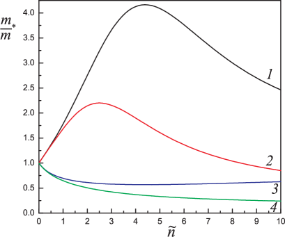
Figure 1: (Color online) Dependencies of the effective mass on density: (1) $\alpha=-2.5$, $u=0$; (2) $\alpha=-2.5$, $u=-0.3$; (3) $\alpha=2.5$, $u=0$; (4) $\alpha=2.5$, $u=1$. It is everywhere assumed that $\lambda=1$.

The total pressure $p=-\Omega\big{/}V$ of the Fermi system with the three-body interaction of the form (6.10) at finite temperatures, according to the general formulae (5.3), (5.4), is as follows

$$p = p_{0}+p_{2}+p_{3},$$

$$p_{0} = \frac{2T}{\Lambda^{3}}\Phi_{5/2}\!\left(\beta\frac{\hbar^{2}k_{\rm F}^{2}}{2m_{*}}\right),\qquad p_{2}=4\pi\!\left[-\!\int_{0}^{\!\infty}\!\!U_{2}(r)\rho^{2}(r)r^{2}\mathrm{d}r+2\rho^{2}(0)\!\int_{0}^{\!\infty}\!\!U_{2}(r)r^{2}\mathrm{d}r\right],$$

$$p_{3} = \!\int\!\!\mathrm{d}{\bf r}\mathrm{d}{\bf r}^{\prime}\,U_{3}(r,r^{\prime},|{\bf r}-{\bf r}^{\prime}|)\!\bigg{[}\!-4\rho(0)\rho^{2}(r^{\prime})+\frac{8}{3}\rho^{3}(0)+\frac{4}{3}\rho(r)\rho(r^{\prime})\rho(|{\bf r}-{\bf r}^{\prime}|)\bigg{]},$$ (8.17)

where the term $p_{0}$ is a contribution of a gas of fermions with the effective mass $m_{*}$, and the terms $p_{2}$ and $p_{3}$ give, respectively, contributions of the pair and three-body interactions. Together with the formula (7.17) for the particle number density, formulae (8) define in a general form the system’s equation of state for the considered form (6.10) of three-body interactions.

At zero temperature, the pressure of the fermion gas

$$\begin{array}[]{ll}\displaystyle{p_{0}=\frac{(3\pi^{2})^{2/3}}{5}\frac{\hbar^{2}}{m_{*}}n^{5/3},}\end{array}$$ (8.18)

and contributions of the pair and three-body forces into the total pressure (8) in the model of ‘‘semi-transparent sphere’’ potentials for them [formulae (6.12), (6.14)], with the expansion formulae (8)–(8.4) taken into account, acquire the form

$$p_{2} = -\frac{U_{2\rm m}n_{*}}{2}\bigg{[}\frac{6}{\pi}\,\tilde{n}\,B_{0}(k_{\rm F}r_{2})-\tilde{n}^{2}\bigg{]},$$ (8.19)

$$p_{3} = 4\rho(0)\bigg{(}\frac{2}{3}b_{1}-b_{2}\bigg{)}+\frac{16\pi}{3}\int_{0}^{\!\infty}\!\!\rho(r)a_{1}\!(r)r^{2}\mathrm{d}r,$$ (8.20)

where $b_{1}$, $b_{2}$, $a_{1}(r)$ are defined by the formulae (8). In the case of densities $n\leqslant n_{*}$, using the expansion

$${B_{n}(z)\approx\frac{z^{n+3}}{9(n+3)}-\frac{z^{n+5}}{45(n+5)}+\frac{z^{n+7}}{525(n+7)}}$$

we find the dependence of the pressure due to the pair interaction on density

$$\frac{p_{2}}{p_{0*}} = \frac{5\,\alpha}{(12\pi^{2})^{1/3}}\bigg{[}\tilde{n}^{2}+\frac{3}{25}\!\left(\frac{9\pi}{4}\right)^{\!2/3}\tilde{n}^{8/3}-\frac{81\pi}{4900}\!\left(\frac{9\pi}{4}\right)^{\!1/3}\tilde{n}^{10/3}\bigg{]}$$ (8.21)

$$= \frac{5\,\alpha}{(12\pi^{2})^{1/3}}\bigg{[}\tilde{n}^{2}+0.442\,\tilde{n}^{8/3}-0.0997\,\tilde{n}^{10/3}\bigg{]}.$$

Here the pressure is related to that of a gas of particles at the characteristic density (8.8): $p_{0*}=$ $\frac{1}{5}{(3\pi^{2})^{2/3}}({\hbar^{2}}/{m})n_{*}^{5/3}$. The sign of pressure (8.21) is determined by the sign of the pair interaction constant and, at negative value of this constant, the interaction contribution into the pressure is negative. The main term in the expansion of pressure due to the three-body interaction (8.20) has the form

$$\frac{p_{3}}{p_{0*}}=\frac{477}{2560}\,\alpha\,u\,\lambda^{8}\,\tilde{n}^{11/3}=0.186\,\alpha\,u\,\lambda^{8}\,\tilde{n}^{11/3}.$$ (8.22)

Attention should be paid to the fact that the expansion of $p_{2}$ holds in even powers of the quantity $\tilde{n}^{1/3}$ and the expansion of $p_{3}$ in odd powers, and the latter begins with a high power.

Since the effective mass depends on density, then the pressure of a gas of quasiparticles (8.18), with account of (8.16), can also be represented in the form of expansion in powers of density:

$$\frac{p_{0}}{p_{0*}} = \tilde{n}^{5/3}+\frac{3}{10}\,\alpha\,\tilde{n}^{8/3}-\frac{3}{70}\!\left(\frac{9\pi}{4}\right)^{\!2/3}\alpha\,\tilde{n}^{10/3}+\frac{159}{2560}\,\alpha\,u\,\lambda^{8}\,\tilde{n}^{11/3}$$ (8.23)

$$= \tilde{n}^{5/3}+0.3\,\alpha\,\tilde{n}^{8/3}-0.158\,\alpha\,\tilde{n}^{10/3}+0.0621\,\alpha\,u\,\lambda^{8}\,\tilde{n}^{11/3}.$$

Taking into account (8.21)–(8.23), we find the expansion of the total pressure in powers of density:

$$\frac{p}{p_{0*}} = \tilde{n}^{5/3}+\frac{5}{(12\pi^{2})^{1/3}}\,\alpha\,\tilde{n}^{2}+\frac{3}{4}\,\alpha\,\tilde{n}^{8/3}-\frac{207}{1960}\!\left(\frac{3\pi^{2}}{2}\right)^{\!1/3}\alpha\,\tilde{n}^{10/3}+\frac{159}{640}\,\alpha\,u\,\lambda^{8}\,\tilde{n}^{11/3}$$ (8.24)

$$= \tilde{n}^{5/3}+1.018\,\alpha\,\tilde{n}^{2}+0.75\,\alpha\,\tilde{n}^{8/3}-0.259\,\alpha\,\tilde{n}^{10/3}+0.248\,\alpha\,u\,\lambda^{8}\,\tilde{n}^{11/3}.$$

Comparison of the accurate dependence of the total pressure on density, calculated by the formulae (8.18)–(8.20) and the approximate dependence, calculated by the formula (8.24), is given in figure 2. It is seen that even at $\tilde{n}\sim 1$, the pressure, calculated by the approximate formula, differs weakly from its accurate value.

Let us discuss the issue of the thermodynamic stability of the Fermi system, assuming $\tilde{n}<1$. For a system to be stable, it is necessary that its compressibility or (which is the same) the squared speed of sound should be positive, so that $\partial p/\partial n>0$. Since in this case the two first terms give the main contribution into the total pressure (8.24) and qualitatively taking into account the new effect of three-body interactions, we find the condition of stability in the form

$$1+\frac{9}{2}\!\left(\frac{4}{9\pi}\right)^{\!2/3}\alpha\,\tilde{n}^{1/3}+\frac{1749}{3200}\,\alpha\,u\,\lambda^{8}\,\tilde{n}^{2}>0.$$ (8.25)

For positive constants of pair and three-body interactions, the system is always stable. More interesting is the case when the constant of the pair interaction is negative. Then, without account of three-body interactions, the condition of stability should be satisfied which can be represented in equivalent forms

$$\tilde{n}^{1/3}<\left(\frac{\pi^{2}}{18}\right)^{\!1/3}|\alpha|^{-1}\approx 0.82\,|\alpha|^{-1},\qquad r_{\textrm{S}}>\left(\frac{18}{\pi^{2}}\right)^{\!1/3}|a_{0}|\approx 1.22\,|a_{0}|.$$ (8.26)

Accounting for the three-body interaction, if it is of a repulsion character, extends the region of stability and can lead to stabilization of the system with the negative pair potential at arbitrary densities in case of fulfilment of the following (8.25) condition

$$\begin{array}[]{ll}\displaystyle{|u|>\frac{200}{583\,\pi^{4}}\frac{5^{5}}{3^{3}}\frac{|\alpha|^{5}}{\lambda^{8}}\approx 0.408\frac{|\alpha|^{5}}{\lambda^{8}}.}\end{array}$$ (8.27)

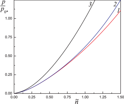
Figure 2: (Color online) Comparison of the accurate dependence of the pressure (1), calculated by the formulae (8.18)–(8.20) and the approximate dependence (2), calculated by the formula (8.24), at $\alpha=-0.3$, $u=-1$, $\lambda=1$. (3) Ideal Fermi gas.

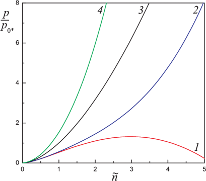
Figure 3: (Color online) Dependencies of the pressure on density: (1) $\alpha=-0.3$, $u=0$; (2) $\alpha=-0.3$, $u=-0.5$; (3) an ideal Fermi gas; (4) $\alpha=0.3$, $u=1$. It is everywhere assumed that $\lambda=1$.

Some dependencies of the pressure on density for different signs of the interparticle interaction are shown in figure 3. In the case of attraction and with neglect of three-body interactions, the spatially uniform state is stable only at low densities for which the condition (8.26) is satisfied. At high densities, the pressure decreases with an increase of density (curve 1 in figure 3) and the spatially uniform state ceases to be stable. Sufficiently intensive three-body repulsive forces lead to stabilization of the system with pair attractive forces (curve 2 in figure 3).

The effect of three-body repulsive forces on the stability of the Fermi system is illustrated more in detail in figure 4. With an increasing strength of the three-body repulsive interaction, the regions of stability of such a system extend (curve 2, 3 in figure 4), and a further growth of the intensity of the three-body interaction leads to stabilization of the system for all physically reasonable values of density.

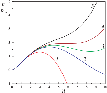
Figure 4: (Color online) The effect of three-body repulsive forces ($U_{3\rm m}>0$) on stability of the Fermi system with pair attractive forces: (1) $u=0$; (2) $u=-0.085$; (3) $u=-0.098$; (4) $u=-0.11$; (5) $u=-0.13$. It is everywhere assumed that $\alpha=-0.3$ and $\lambda=1$.

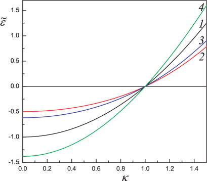
Figure 5: (Color online) The quasiparticle energy spectrum $\tilde{\varepsilon}(\kappa)$ (in the variables $\tilde{\varepsilon}\equiv\varepsilon_{k}/\varepsilon_{\rm F}$, $\kappa\equiv k/k_{\rm F}$): (1) Ideal Fermi gas [$\tilde{\varepsilon}(\kappa)=\kappa^{2}-1$, $\tilde{m}_{*}\equiv m_{*}/m=1$];  (2) $\alpha=-2.5$, $u=0$, $\tilde{n}=1$ ($\tilde{m}_{*}=1.78$); (3) $\alpha=-2.5$, $u=-1$, $\lambda=1$, $\tilde{n}=1$ ($\tilde{m}_{*}=1.50$);  (4) $\alpha=2.5$, $u=-1$, $\lambda=1$, $\tilde{n}=1$ ($\tilde{m}_{*}=0.75$).

The form of the quasiparticle energy spectrum with account of the interparticle interactions is shown in figure 5. Accounting for only the pair attraction leads to a slowing down of the energy increase with increasing momentum relative to an ideal Fermi gas (curve 2 in figure 5). Accounting for the repulsive three-body forces, against the background of the attractive pair forces, additionally yields a small increase of the quasiparticle energy (curve 3 in figure 5). The effect of three-body forces on the spectrum is appreciably weaker than the role of pair forces, so that accounting for the attractive three-body forces in the presence of the pair repulsion weakly prevents the increase of the quasiparticle energy as momentum increases (curve 4 in figure 5).

9 Conclusion

The self-consistent field equations are obtained, and, within this model, thermodynamic relations are derived for a normal system of Fermi particles with account of both pair and three-body forces. The satisfaction of the essential requirement of fulfilment of all thermodynamic relations already in the self-consistent approximation leads to a unique formulation of the self-consistent field model. Emphasized are the novelty and universality of the proposed approach to the formulation of this model and the usefulness of the method for describing not only Fermi, but also Bose systems, in particular phonons, and relativistic quantized fields. The approach being developed allows us also, as shown in the paper, to account for many-body interactions naturally.

It is shown that three-body interactions of zero radius give no contribution into the self-consistent field and, in order to account for the effects due to such interactions, it is necessary to account for their nonlocality. The case of the spatially uniform system is considered in detail. General formulae are derived for the system’s equation of state and the effective mass of quasiparticles with account of three-body forces. Dependencies of the quasiparticle effective mass and the system’s pressure on density at zero temperature are obtained, with pair and three-body forces accounted for in the model of interaction potentials of ‘‘semi-transparent sphere’’ type.

It is shown that pair interactions of repulsive character reduce the quasiparticle effective mass relative to the mass of a free particle while attractive pair interactions, on the contrary, raise it. The effective mass and pressure are numerically calculated at zero temperature and expansions of these quantities are derived in powers of the relative density with account of three-body forces. It is shown that the relative contribution of three-body interactions into thermodynamic quantities rises with an increasing density. The effect of three-body forces on the stability of the Fermi system is considered, and it is shown that in the case of repulsion, their being taken into account extends the region of stability and can lead to stabilization of the system with pair attraction. The quasiparticle energy spectrum is calculated with account of the interparticle interactions.

Ukrainian 0 Модель самоузгодженого поля для фермi-систем
з врахуванням тричастинкових взаємодiй Ю.М. Полуектов, О.О. Сорока, С.М. Шульга

             
Iнститут теоретичної фiзики iм. О.I. Ахiєзера, ННЦ ХФТI, вул. Академiчна, 1, 61108 Харкiв, Україна

References

• [1] Kirzhnits D.A., Field Theoretical Methods in Many-Body systems, Pergamon, Oxford, 1967.
• [2] Eisenberg J., Greiner W., Microscopic Theory of the Nucleus, North-Holland, London, 1972.
• [3] Barts B.I., Bolotin Yu.L., Inopin E.V., Gonchar V.Yu., The Hartree-Fock Method in Nuclear Theory, Naukova Dumka, Kiev, 1982 (in Russian).
• [4] Hartree D.R., The Calculation of Atomic Structures, Wiley, New York, 1957.
• [5] Slater J.C., The Self-Consistent Field for Molecules and Solids, McGraw-Hill, New York, 1974.
• [6] Braut R., Phase Transitions, Benjamin, New York, 1965.
• [7] Vaks V.G., Larkin A.I., Pikin S.A., Sov. Phys. JETP, 1967, 24, 240.
• [8] Poluektov Yu.M., Low Temp. Phys., 1997, 23, 685; doi:10.1063/1.593364.
• [9] Poluektov Yu.M., Bulletin of Kharkiv National University, Phys. Ser. ‘‘Nuclei, particles, fields’’, 2001, 522, 3.
• [10] Poluektov Yu.M., Ukr. J. Phys., 2005, 50, 1303; Preprint arXiv:1303.4913, 2013.
• [11] Poluektov Yu.M., Ukr. J. Phys., 2015, 60, 553.
• [12] Landau L.D., Sov. Phys. JETP, 1957, 3, 920.
• [13] Pines D., Nozières P., The Theory of Quantum Liquids, Benjamin, New York, 1966.
• [14] Migdal A.B., Theory of Finite Fermi Systems and Applications to Atomic Nuclei, Nauka, Moscow, 1983 (in Russian).
• [15] Kolomiets V.M., Nuclear Fermi-Liquid, Naukova Dumka, Kiev, 2009 (in Russian).
• [16] Akhiezer A.I., Krasil’nnikov V.V., Peletminskii S.V., Yatsenko A.A., Phys. Rep., 1994, 245, 1;
doi:10.1016/0370-1573(94)90060-4.
• [17] Poluektov Yu.M., Fiz. Nizk. Temp., 1995, 21, 300 (in Russian).
• [18] Poluektov Yu.M., Fiz. Nizk. Temp., 1996, 22, 402 (in Russian).
• [19] Axilrod B.M., Teller E., J. Chem. Phys., 1943, 11, 299; doi:10.1063/1.1723844.
• [20] Basu A.N., Sengupta S., Phys. Status Solidi B., 1968, 29, 367; doi:10.1002/pssb.19680290137.
• [21] Sarkar A.K., Sengupta S., Solid State Commun., 1969, 7, 135; doi:10.1016/0038-1098(69)90710-8.
• [22] Bethe H.A., Ann. Rev. Nucl. Sci., 1971, 21, 93; doi:10.1146/annurev.ns.21.120171.000521.
• [23] Skyrme T.H.R., Nucl. Phys., 1959, 9, 615; doi:10.1016/0029-5582(58)90345-6.
• [24] Vautherin D., Brink D.M., Phys. Rev. C, 1972, 5, 626; doi:10.1103/PhysRevC.5.626.
• [25] Hammer H.-W., Nogga A., Schwenk A., Rev. Mod. Phys., 2013, 85, 197; doi:10.1103/RevModPhys.85.197.
• [26] Landau L.D., Lifshitz E.M., Quantum Mechanics, Pergamon Press, 1977.
• [27] Poluektov Yu.M., Low Temp. Phys., 2002, 28, 429; doi:10.1063/1.1491184.
• [28] Poluektov Yu.M., Ukr. J. Phys., 2007, 52, 579; Preprint arXiv:1306.2103, 2013.
• [29] Poluektov Yu.M., Fiz. Nizk. Temp., 2015, 41, 1181 (in Russian) [Low Temp. Phys., 2015, 41, 922; doi:10.1063/1.4936228].
• [30] Poluektov Yu.M., Bulletin of Kharkiv National University, Phys. Ser. ‘‘Nuclei, particles, fields’’, 2009, 859, 9; Preprint arXiv:1507.00246v2, 2015.
• [31] Poluektov Yu.M., Russ. Phys. J., 2010, 53, 163; doi:10.1007/s11182-010-9401-6.
• [32] Bogoliubov N.N., Bogoliubov N.N. (jr), Introduction to Quantum Statistical Mechanics, World Scientific PC, Singapore, 2009.
• [33] Sarry A.M., Sarry M.F., Tech. Phys., 2014, 59, 474; doi:10.1134/S1063784214040215.
• [34] Gale J.D., J. Chem. Soc., Faraday Trans., 1997, 93, 629; doi:10.1039/A606455H.
• [35] Thouless D.J., The Quantum Mechanics of Many-Body Systems, Academic Press, New York, 1972.
• [36] Bazarov I.P., Statistical Theory of the Crystalline State, Moscow University Press, Moscow, 1972 (in Russian).
• [37] Pitaevskii L.P., Stringari S., Bose-Einstein Condensation, Oxford University Press, Oxford, 2003.
• [38] Aziz R.A., Slaman M.J., J. Chem. Phys., 1991, 94, 8047; doi:10.1063/1.460139.
• [39] Anderson J.B., Traynor C.A., Boghosian B.M., J. Chem. Phys., 1993, 99, 345; doi:10.1063/1.465812.
• [40] McDougall J., Stoner E.C., Phil. Trans. Roy. Soc. A, 1938, 237, 67; doi:10.1098/rsta.1938.0004.
• [41] Varshalovich D.A., Moskalev A.N., Khersonskii V.K., Quantum Theory of Angular Momentum, Nauka, Leningrad, 1975 (in Russian).
\@nopatterns
Ukrainian \adddialect\l@ukrainian0 \l@ukrainian Модель самоузгодженого поля для фермi-систем