Magnetic spheres in microwave cavities

Abstract

We apply Mie scattering theory to study the interaction of magnetic spheres with microwaves in cavities beyond the magnetostatic and rotating wave approximations. We demonstrate that both strong and ultra-strong coupling can be realized for a stand alone magnetic spheres made from yttrium iron garnet (YIG), acting as an efficient microwave antenna. The eigenmodes of YIG spheres with radii of the order mm display distinct higher angular momentum character that has been observed in experiments.

I Introduction

Light-matter interaction in the strong coupling regime is an important subject in coherent quantum information transfer.Wallraff2004 ; Kubo2010 ; Putz2014 Spin ensembles such as nitrogen-vacancy centers may couple strongly to electromagnetic fields and have the advantage of both long coherence times Bar-Gill2013 and fast manipulation Childress2006 . The “magnon” refers to the collective excitation of spin systems. In paramagnetic spin ensembles in an applied magnetic field, the spins precess coherently in the presence of microwave radiation, creating hybridized states referred to as magnon-polaritons.Mills1974 ; Lehmeyer1985 ; Cao In the strong coupling regime coherent energy exchange exceeds the dissipative loss of both subsystems. The coherent coupled systems is usually described by the Tavis-Cummings (TC) model Tavis1968 ; Fink2009 , which defines a coupling constant $g$ between the spin-ensemble and the electromagnetic radiation that scales with the square root of the number of spins. In ferro/ferrimagnets the net spin density is exceptionally large and spontaneously ordered, which makes those materials very attractive for strong-coupling studies. The exchange coupling of spins in magnetic materials also strongly modifies the excitation spectrum into a spectrum or spin wave band structure. An ubiquitous experimental technique to study ferromagnetism is ferromagnetic resonance (FMR), i.e. the absorption, transmission or reflection spectra of microwaves. In the weak coupling regime FMR gives direct access to the elementary excitation spectrum of ferromagnets,Hillebrands including the standing spin waves in confined systems referred to spin wave resonance (SWR).SWR The strong coupling regime is studied less frequently, however, because the dissipative losses of the magnetization dynamics are usually quite large.

An exceptional magnetic material is the man-made yttrium iron garnets (YIG), a ferrimagnetic insulator. Commercially produced high-quality spherical YIG samples serve in magnetically tunable filters and resonators at microwave frequencies. By suitable doping becomes a versatile class of materials with low dissipation and unique microwave properties Serga2010 . YIG has spin density of $2\times 10^{22}\mathrm{cm}^{-3}$, Gilleo1958 and the Gilbert damping (reciprocal quality) factor of the magnetization dynamics ranges from $10^{-5}$ to $10^{-3}$ Kajiwara2010 ; Heinrich2011 ; Kurebayashi2011 , which facilitates strong coupling for smaller samples. Indeed, strongly coupled microwave photons with magnons have been experimentally reported for either YIG films with broadband coplanar waveguides (CPWs)Huebl2013 ; Stenning2013 ; Bhoi2014 , or YIG spheres in 3D microwave cavities Tabuchi2014 ; Zhang2014 ; Goryachev2014 . A series of anticrossings were observed in thicker YIG films and split rings Stenning2013 ; Bhoi2014 . The coupling of magnons in YIG spheres with a superconducting qubit via a mircowave cavity mode in the quantum limit has been reported Tabuchi2014 . An ultrahigh cooperativity $C=g^{2}/\kappa\gamma>10^{5},$ where $\kappa$ and $\gamma$ are the loss rates of the cavity and spin system, and multimode strong coupling were found at room Zhang2014 as well as the low Goryachev2014 temperatures.

From a theoretical point of view, the standard TC model is too simple to describe the full range of coupling between magnets and microwaves. Also the rotating-wave approximation (RWA) (usually but not necessarily assumed in the TC model) is speaking applicable when the coupling ratio $g/\omega_{c}\ll 1$, where $\omega_{c}$ is the microwave cavity mode frequency. We may define different coupling regimes Ballester2012 ; Moroz2014 , viz. (i) strong coupling (SC) when $0.01<g/\omega_{c}\lesssim 0.1$, (ii) ultrastrong coupling (USC) Niemczyk2010 when $g/\omega_{c}\gtrsim 0.1$, (iii) or even deep strong coupling (DSC) $g/\omega_{c}\approx 1$ Casanova2010 . Cao et al. Cao adapted the TC model to ferromagnets by formulating a first-principles scattering theory of the coupled cavity-ferromagnet system based on the Maxwell and the Landau-Lifshitz-Gilbert equation including the exchange interaction. A effectively one-dimensional system of a thin film with in-plane magnetization in a planar cavity was solved exactly in the linear regime, exposing, for example, strong-coupling to standing spin waves. Maksymov et al. Maksymov carried out a numerical study of the strong coupling regime in all-dielectric magnetic multilayers that resonantly enhance the microwave magnetic field. A quantum theory of strong coupling for nanoscale magnetic spheres in microwave resonators has been developed in the macrospin approximation Soykal2010 , but this regime has not yet been reached in experiments.

Here we apply our classical method Cao to spherically symmetric systems, i.e., a magnetic sphere in the center of a spherical cavity. This is basically again a one-dimensional problem that can be treated semi-analytically and has other advantages as well, such as a homogeneous dipolar field and simple boundary conditions. The eigenmodes of magnetic spheres have been studied in the “magnetostatic” approximation Walker ; Fletcher1959 , in which the spins interact by the magnetic dipolar field, disregarding exchange as well as propagation effects, which may be done when $\lambda\gg a$, where $a$ is the radius of the sphere and $\lambda$ the wavelength of the incident radiation. Arias et al. Arias2005 treated the interaction of magnetic spheres with microwaves in the weak-coupling regime. In contrast, we address here the properties of the fully hybridized magnon-polaritons beyond the magnetostatic approximation (but disregard the exchange interaction), including the propagation effects (reflection and transmission) of microwaves, thereby extending the validity to $\lambda<a$. We are admittedly still one step from the “exact” solution by disregarding the exchange (as treated and discussed by Cao et al. Cao ). Our calculated microwave spectra are complex but help in understanding some of the above-mentioned experiments.

This manuscript is organized as follows. In Sec. II, we introduce the details of our model and derive the scattered intensity and efficiency factors for a strongly coupled system of a magnetic sphere and microwaves. In Sec. III, we present and discuss our numerical results that demonstrate the effects both due to the dielectric as well as magnetic effects on the scattering properties and compare our results with experiments. In Sec. IV, we conclude and summarize our findings.

II Model and formalism

We model the coupling of the collective excitations of a magnetic sphere to microwaves in a spherical cavity by the coupled Landau-Lifshitz-Gilbert and Maxwell equations. We employ Mie-type scattering theory, i.e., a rapidly converging expansion into spherical harmonics Mie ; Kerker ; Stratton . We model the incoming radiation as plane electromagnetic waves with arbitrary polarization and wave vector that are scattered by a cavity loaded by a magnetic sphere with gyromagnetic permeability tensor $\overleftrightarrow{\mu}.$Gerson1974 In order to understand the experiments it is not necessary to precisely model the details of the resonant cavity. Instead, we propose a generic model cavity that is flexible enough to mimic any realistic situation by adjusting the parameters. We consider a thin spherical shell of a material with high dielectric constant $\epsilon_{c}/\epsilon_{0}\gg 1,$ radius $R$, and thickness $\delta$ that confines standing microwave modes with adjustable interaction with the microwave source (see Fig. 1). The spherical symmetry simplifies the mathematical treatment, while the parameters $R$ and $\delta$ allow us to freely tune the frequencies and broadenings of the cavity modes.

The dynamics of the magnetization vector $\mathbf{M}$ is described by the LLG equation,

$$\partial_{t}\mathbf{M}=-\gamma\mathbf{M}\times\mathbf{H}_{\mathrm{eff}}+\frac{\alpha}{M_{s}}\mathbf{M}\times\partial_{t}\mathbf{M}$$ (1)

with $\alpha$ and $\gamma$ being the Gilbert damping constant and gyromagnetic ratio, respectively. The effective magnetic field $\mathbf{H}_{\mathrm{eff}}=\mathbf{H}_{\mathrm{ext}}+\mathbf{H}_{\mathrm{x}}$ comprises the external and (collinear) easy axis anisotropy fields $\mathbf{H}_{\mathrm{ext}}$ as well as the exchange field $\mathbf{H}_{\mathrm{x}}=J\nabla^{2}\mathbf{M}$, with $J$ being the exchange stiffness. Assuming that perturbing microwave magnetic field and magnetization precession angles are small:

$$\mathbf{M}(\mathbf{r},t) =\mathbf{M}_{s}+\mathbf{m}(\mathbf{r},t)$$ (2)

$$\mathbf{H}(\mathbf{r},t) =\mathbf{H}_{\mathrm{ext}}+\mathbf{h}(\mathbf{r},t)$$ (3)

where $\mathbf{M}_{s}$ is the saturated magnetization vector and $\mathbf{m}$ the small-amplitude magnetization driven by the rf magnetic field $\mathbf{h,}$ we linearize the LLG equation to

$$\partial_{t}\mathbf{m}=-\gamma\mathbf{M}_{s}\times\left(\mathbf{H}_{\mathrm{eff}}^{(1)}-\frac{\alpha}{\gamma M_{s}}\partial_{t}\mathbf{m}\right)-\gamma\mathbf{m}\times\mathbf{H}_{\mathrm{eff}}^{(0)}$$ (4)

where $\mathbf{H}_{\mathrm{eff}}^{(0)}=\mathbf{H}_{\mathrm{ext}}$ and $\mathbf{H}_{\mathrm{eff}}^{(1)}=\mathbf{H}_{\mathrm{x}}+\mathbf{h}$. The response of ferromagnetic spheres is affected by exchange when their radii approach the exchange length. Since the latter is typically a few $\mathrm{nm}$, we hereafter disregard the exchange interaction and concentrate on the dipolar spin waves. In the frequency domain and taking the $\mathbf{z}$ direction as the equilibrium direction for the magnetization,

$$i\omega\mathbf{m}=\mathbf{z}\times\left(\omega_{\mathrm{M}}\mathbf{h}-\omega_{\mathrm{H}}\mathbf{m}+i\omega\alpha\mathbf{m}\right),$$ (5)

with $\omega_{\mathrm{M}}=\gamma M_{s}$ and $\omega_{\mathrm{H}}=\gamma H_{0}$. We may recast Eq. (6) into the form $\mathbf{m}=\overleftrightarrow{\chi}\cdot\mathbf{h.}$The magnetic susceptibility tensor $\overleftrightarrow{\chi}$ is related to the magnetic permeability tensor by $\overleftrightarrow{\mu}=\mu_{0}(\overleftrightarrow{1}+\overleftrightarrow{\chi})$. We find

$$\overleftrightarrow{\mu}=\mu_{0}\begin{pmatrix}1+\chi&-i\kappa&0\\ i\kappa&1+\chi&0\\ 0&0&1\end{pmatrix}$$ (6)

where $\chi$ and $\kappa$ are given by,

$$\chi =\frac{(\omega_{\mathrm{H}}-i\alpha\omega)\omega_{\mathrm{M}}}{(\omega_{\mathrm{H}}-i\alpha\omega)^{2}-\omega^{2}}$$ (7)

$$\kappa =\frac{\omega\omega_{\mathrm{M}}}{(\omega_{\mathrm{H}}-i\alpha\omega)^{2}-\omega^{2}}.$$ (8)

The permeability tensor appears in the Maxwell equations for the propagation of the electromagnetic wave in a magnetic medium.

Inside a spatially homogeneous medium a monochromatic wave with frequency $\omega$,

$$\mathbf{\nabla}\times\mathbf{E} =i\omega\mathbf{b},\quad\mathbf{\nabla}\times\mathbf{h}=-i\omega\mathbf{D}$$ (9)

$$\mathbf{\nabla}\cdot\mathbf{D} =0,\qquad\quad\mathbf{\nabla}\cdot\mathbf{b}=0.$$ (10)

The constitutive relation between the magnetic induction $\mathbf{b}$, electric displacement $\mathbf{D}$, magnetic field $\mathbf{h}$, and the electric field $\mathbf{E}$ inside this medium are

$$\mathbf{b}=\overleftrightarrow{\mu}\cdot\mathbf{h},\quad\mathbf{D}=\epsilon_{\mathrm{sp}}\mathbf{E}.$$ (11)

where $\epsilon_{\mathrm{sp}}$ is the scalar permittivity of the medium. It follows from Eqs. (10) and (11) that the magnetic induction $\mathbf{b}$ satisfies the wave equation,

$$\mathbf{\nabla}\times\mathbf{\nabla}\times(\mu_{0}\overleftrightarrow{\mu}^{-1}\cdot\mathbf{b})-k_{\mathrm{sp}}^{2}\mathbf{b}=0$$ (12)

with $k_{\mathrm{sp}}^{2}=\omega^{2}\epsilon_{\mathrm{sp}}\mu_{0}$.

The surrounding (nonmagnetic) medium is homogeneous and isotropic with scalar magnetic permeability $\mu_{0}$, divergenceless magnetic field, and simplified wave equation $\mathbf{\nabla}^{2}\mathbf{b}+k_{\mathrm{sp}}^{2}\mathbf{b}=0$. Due to the spherical symmetry it is advantageous to expand the magnetic field $\mathbf{h}$ into vector spherical harmonics as Kerker ; Stratton ; ZLin ; LWL

$$\mathbf{h}=\sum_{nm}\bar{\eta}_{nm}\left[p_{nm}\mathbf{M}_{nm}^{(1)}(k,\mathbf{r})+q_{nm}\mathbf{N}_{nm}^{(1)}(k,\mathbf{r})\right],$$ (13)

where $n$ runs from 1 to $\infty$, and $m=-n,\cdots,n$ with prefactors $\bar{\eta}_{nm}=\eta_{nm}k_{0}/(\omega\mu_{0})$,

$$\eta_{nm}=i^{n}E_{0}\left[\frac{2n+1}{n(n+1)}\frac{(n-m)!}{(n+m)!}\right]^{1/2}.$$ (14)

$E_{0}$ is the electric field amplitude of the incident wave . The vector spherical harmonics read Kerker ; Stratton ; ZLin ; LWL

$$\mathbf{M}_{nm}^{(j)}(k,\mathbf{r}) =z_{n}^{(j)}(kr)\mathbf{X}_{nm}(\hat{\mathbf{r}}),$$

$$k\mathbf{N}_{nm}^{(j)}(k,\mathbf{r}) =\mathbf{\nabla}\times\mathbf{M}_{nm}^{(j)}(k,\mathbf{r}).$$ (15)

$z_{n}^{(j)}(kr)$ are spherical Bessel functions, $\mathbf{X}_{nm}(\hat{\mathbf{r}})=\mathbf{L}Y_{nm}(\hat{\mathbf{r}})/\sqrt{n(n+1)}$ spherical harmonics and $\mathbf{L}=-i\mathbf{r}\times\mathbf{\nabla}_{\mathbf{r}}$ the angular momentum operator with $\mathbf{\nabla}_{\mathbf{r}}$ the gradient operator. The electric field distribution is obtained by $\mathbf{E}=(i/\omega c)\mathbf{\nabla}\times\mathbf{h}$. By invoking the vector spherical wave function expansion for $\mathbf{b}$ and $\overleftrightarrow{\mu}^{-1}\cdot\mathbf{b}$ in the wave equation Eq. (12) leads to the dispersion relation for $k\left(\omega\right)$.

We match the field distributions inside and outside the cavity to obtain the scattering solution for incident plane microwaves. The field inside the spherical shell must be regular, while the scattered component has to satisfy the scattering wave boundary conditions at infinity. These conditions are fulfilled by adopting the first kind of spherical Bessel function $j_{n}(x)$ as radial part for the internal distribution and the first kind of spherical Hankel function $h_{n}^{(1)}(x)$ for the scattered component outside the cavity

$$\mathbf{h}_{s}=\sum_{nm}\bar{\eta}_{nm}\left[c_{nm}\mathbf{N}_{nm}^{(3)}(k_{0},\mathbf{r})+d_{nm}\mathbf{M}_{nm}^{(3)}(k_{0},\mathbf{r})\right].$$ (16)

The unknown scattering coefficients $c_{nm}$ and $d_{nm}$ are determined by the boundary conditions at the interface. We consider here the situation in which the magnetic sphere is illuminated by a plane wave with arbitrary direction of propagation and polarization as indicated in Fig. 1. The incident field can be expanded as

$$\mathbf{h}_{inc}=-\sum_{nm}\bar{\eta}_{nm}\left[u_{nm}\mathbf{N}_{nm}^{(1)}(k_{0},\mathbf{r})+v_{nm}\mathbf{M}_{nm}^{(1)}(k_{0},\mathbf{r})\right].$$ (17)

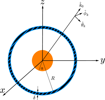
Figure 1: (Color online) Plane wave with wave vector $\mathbf{k}_{0}$ coming in at an arbitrary angle hits a large spherical cavity modeled by a dielectric spherical shell of radius $R$, thickness $\delta$, and permittivity $\epsilon_{c}$. The spherical cavity is loaded with a magnetic sphere of radius $a$ centered at the origin of the coordinate system.

The expansion coefficients $u_{mn}$ and $v_{mn}$,

$$u_{nm} =\left[p_{\theta}\tilde{\tau}_{nm}(\cos\theta_{k})-ip_{\phi}\tilde{\pi}_{nm}(\cos\theta_{k})\right]e^{-im\phi_{k}},$$ (18)

$$v_{nm} =\left[p_{\theta}\tilde{\pi}_{nm}(\cos\theta_{k})-ip_{\phi}\tilde{\tau}_{nm}(\cos\theta_{k})\right]e^{-im\phi_{k}},$$ (19)

contain all information about the polarization vector and direction of propagation, where $\hat{\mathbf{p}}=(p_{\theta}\hat{\theta}_{k}+p_{\phi}\hat{\phi}_{k})$ is the normalized complex polarization vector, with $\left|\hat{\mathbf{p}}\right|=1$ and $\theta_{k}(\phi_{k})$ is the polar (azimuthal) angle of $\mathbf{k}_{0}$. Two auxiliary functions are defined by

$$\tilde{\pi}_{nm}=t_{nm}\frac{m}{\sin\theta}P_{n}^{m}(\cos\theta),\leavevmode\nobreak\ \tilde{\tau}_{nm}=t_{nm}\frac{d}{d\theta}P_{n}^{m}(\cos\theta),$$ (20)

with $t_{nm}=i^{-n}\eta_{nm}/E_{0}$ and $P_{n}^{m}(x)$ the first kind associated Legendre function.

In order to solve the full scattering problem including the cavity we match the fields outside the cavity caused by the incoming plane microwave and the spacer region separating the magnetic particle and cavity. In the latter, spherical Bessel functions of both the first and second kind have to be included into the expansion. At the surface of the magnetic sphere $\left(r=a\right)$ we adopt the standard boundary conditions

$$\mathbf{h}_{i}\times\mathbf{e_{r}} =\mathbf{h}_{mid}\times\mathbf{e_{r}}$$ (21)

$$\mathbf{\mathbf{E}}_{i}\times\mathbf{e_{r}} =\mathbf{\mathbf{E}}_{mid}\times\mathbf{e_{r}}$$ (22)

while at the surface of the cavity, assuming that its thickness is much smaller than the wavelength,MGA-57-1 ; MGA-57-2

$$\left[\mathbf{h}_{mid}-\mathbf{h}_{out}\right]\times\mathbf{e_{r}} =-\xi\left[\mathbf{e_{r}}\times\mathbf{\mathbf{E}}_{out}\right]\times\mathbf{e_{r},}$$ (23)

$$\mathbf{\mathbf{E}}_{mid}\times\mathbf{e_{r}} =\mathbf{\mathbf{E}}_{out}\times\mathbf{e_{r}.}$$ (24)

The indexes mid and out indicate the regions within and outside of the cavity, respectively. The unit vector $\mathbf{e_{r}}$ is the outward normal to the surfaces and $\xi=i\omega(\epsilon_{c}-\epsilon_{0})\delta$ with permittivity of the cavity shell $\epsilon_{c}$. By matching the field distributions in the different regions the scattering coefficients are determined, from which we calculate the observables.

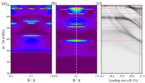
Figure 2: (Color online) Scattering intensity $|S_{1}|^{2}$ as function of scattering angle $\theta$ and frequency $\omega/2\pi$ is shown for (a) a dielectric sphere of radius $a=1.25\,\mathrm{mm}$ and relative permittivity $\epsilon/\epsilon_{0}=15$ and for (b) the same sphere in a cavity of radius $R=1.6\,\,\mathrm{mm}$. In (c) the scattering intensity is plotted for the same cavity as function of frequency and loading rate $a/R$. The dashed lines are guides for the eye.

At distances sufficiently far from the cavity, i.e., in the far field zone, the intensity of the two polarization components $I_{1}$ and $I_{2}$ are

$$I_{1} \sim\frac{E_{0}^{2}}{k_{0}^{2}r^{2}}|S_{1}(\theta,\phi)|^{2},$$ (25)

$$I_{2} \sim\frac{E_{0}^{2}}{k_{0}^{2}r^{2}}|S_{2}(\theta,\phi)|^{2}.$$ (26)

where $\theta\leavevmode\nobreak\ (\phi)$ is the polar (azimuthal) angle of the observer at distance $r$. The scattering amplitude functions are

$$S_{1}(\theta,\phi) =\sum_{nm}\left[d_{nm}\tilde{\tau}_{nm}(\cos\theta)+c_{nm}\tilde{\pi}_{nm}(\cos\theta)\right]e^{im\phi},$$ (27)

$$S_{2}(\theta,\phi) =\sum_{nm}\left[d_{nm}\tilde{\pi}_{nm}(\cos\theta)+c_{nm}\tilde{\tau}_{nm}(\cos\theta)\right]e^{im\phi},$$ (28)

where the coefficients $c_{nm}$ and $d_{nm}$ characterize the scattered component of the fields outside the cavity. We may now compute the scattering and extinction cross sections as well as their (dimensionless) efficiencies $Q_{sca}$ and $Q_{ext}$, which are the cross sections normalized by $\pi R^{2}$, the geometrical cross section of the cavity:

$$Q_{sca} =\dfrac{4}{k_{0}^{2}R^{2}}\sum_{nm}\left(|c_{nm}|^{2}+|d_{nm}|^{2}\right),$$ (29)

$$Q_{ext} =\dfrac{4}{k_{0}^{2}R^{2}}\sum_{nm}\mathrm{Re}\left(u_{nm}^{\ast}d_{nm}+v_{nm}^{\ast}c_{nm}\right).$$ (30)

The extinction cross section represents the ratio of (angle-integrated) emitted to incident intensity, i.e., with and without the scattering cavity/particle between source and detector. This factor measures the energy loss of the incident beam by absorption and scattering. The series expansion in Eqs. (27)-(30) is uniformly convergent and can be truncated at some point in numerical calculations depending on the desired accuracy. In the next section we present our results with emphasis on the dielectric and magnetic contributions to the microwave scattering.

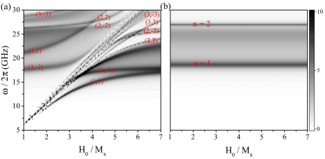
Figure 3: (Color online) Panel (a) shows the scattering efficiency factor $Q_{sca}$ as function of normalized magnetic field $H_{0}/M_{s}$ and frequency $\omega/2\pi$ for a YIG sphere of radius $a=2\,\mathrm{mm}$ and relative permittivity $\epsilon/\epsilon_{0}=15$. Panel (b) shows results for a non-magnetic dielectric sphere. The character of the microwave modes sufficiently far from the anti-crossing with the spin waves is labeled by the spherical harmonic indices $(n,m)$.

III Results

Here we present numerical results on the coupling of microwaves with a ferro- or ferrimagnet in a cavity based on our treatment of Mie scattering of the electromagnetic waves as exposed in the preceding section. It applies to a dielectric/magnetic sphere centered in a (larger) spherical cavity, but both may be of arbitrary diameter otherwise. We are mainly interested in the coherent coupling between the magnons and microwave photons in the strong or even ultrastrong coupling regimes that can be achieved by generating spectrally sharp cavity modes, by increasing the filling factor of the cavity, or simply by increasing the size of the sphere. The RWA, however, tends to break down as the coupling increases. This has led to different coupling regimes beyond the weak coupling, TC region, i.e., strong (SC) and ultrastrong (USC) coupling regimes. In the SC region coupling strength has to be comparable or larger than all decoherence rates, while in the USC it has to be comparable or larger than appreciable fractions of the mode frequency, $g/\omega_{c}\gtrsim 0.1$.

We adopt the forward scattered intensities $I_{1}\sim|S_{1}(\theta=\pi/2,\phi=\pi)|^{2}$ and scattering efficiency factors as convenient and observable measures of the microwave scattering by a spherical target. In order to compare results with recent experiments, we chose parameters for YIG with gyromagnetic ratio $\gamma/(2\pi)=28\leavevmode\nobreak\$ GHz/T, saturation magnetization Grishin $\mu_{0}M_{s}=175\leavevmode\nobreak\$ mT, Gilbert damping constantKajiwara2010 ; Heinrich2011 ; Kurebayashi2011 $\alpha=3\times 10^{-4}$, and relative permittivity Murthy $\epsilon/\epsilon_{0}=15.$ Without loss of generality we consider microwaves incident from the positive $x$ direction ($\theta_{k}=\pi/2$ and $\phi_{k}=0$) and polarization $(p_{\theta},p_{\phi})=(1,0)$, so its electric/magnetic components are in the $-$$z/y$ directions (static magnetic field and magnetization $\mathbf{H}_{0}\|\mathbf{z}$). Forward scattering is monitored by setting $\theta=\pi/2$ and $\phi=\pi$ in Eq. (27). We also explore the dependence of the observables on the scattering angles. We can remove the cavity simply by setting $\xi=0$.

In Fig. 2 the scattered intensity $|S_{1}(\theta,\pi)|^{2}$ is depicted as a function of frequency $\omega/2\pi$ and scattering angle $\theta$ focusing first on a non-magnetic sphere with radius $a=1.25\,\mathrm{mm}$. The angular dependence of the scattering with and without a cavity (with $R=1.6\,\mathrm{mm)}$ is plotted in panel (a) and (b), respectively. The eigenmodes of the dielectric sphere show $s$, $p$ and $d$-wave characters in Fig. 2(a). $s$-wave scattering dominates as long as the wavelength (reduced by $\epsilon_{\mathrm{sp}}$) does not fit twice into the sphere, i.e., $\lambda\gtrapprox a\sqrt{\epsilon_{\mathrm{sp}}/\epsilon_{0}}$. The spherical cavity, on the other hand, limits the isotropic scattering regime to $\lambda\gtrapprox R\sqrt{\epsilon_{\mathrm{sp}}/\epsilon_{0}}$.

In Fig. 2(c) we plot the forward scattered intensities $I_{1}$ as function of the load of the cavity by a dielectric sphere. The eigenfrequencies of the cavity remain constant, while those confined to the sphere shift to lower frequencies as $\sim a^{-2}$. At high loading rate the cavity modes are strongly mixed with the modes in the sphere and all of them bend towards lower frequencies.

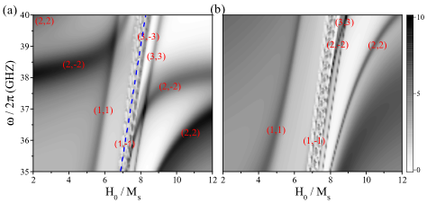
Figure 4: (Color online) Scattering efficiency factor $Q_{sca}$ plotted as function of normalized magnetic field $H_{0}/M_{s}$ and frequency $\omega/2\pi$ for a YIG sphere of radius $a=1.25\,\mathrm{mm}$ and relative permittivity $\epsilon/\epsilon_{0}=15$ (a) in the center of a spherical cavity of radius $R=1.6\,\mathrm{mm}$ and (b) without cavity.

Magnetism of the spheres can affect the microwave scattering properties strongly, but the issue of hybridization of cavity and sphere resonant microwave modes is still present. A sufficiently large YIG sphere alone can therefore provide strong coupling conditions to the magnetization even without an external resonator. To this end, the linear dimension of the YIG sphere must be of a size that allows the internal resonances of the sphere to come into play in the microwave frequency range, i.e. when $ka\gtrapprox\pi\sqrt{\epsilon_{0}/\epsilon_{\mathrm{sp}}}$ or $\lambda\lessapprox 2a\sqrt{\epsilon_{\mathrm{sp}}/\epsilon_{0}}$. We therefore have a (narrow) regime $a\sqrt{\epsilon_{\mathrm{sp}}/\epsilon_{0}}\lessapprox\lambda\lessapprox 2a\sqrt{\epsilon_{\mathrm{sp}}/\epsilon_{0}}$ or $7.75\,\mathrm{mm}\lessapprox\lambda\lessapprox 15.49\,\mathrm{mm}$ (for Fig.3) in which strong coupling and $s$-wave scattering can be realized simultaneously without a cavity. YIG spheres can typically be fabricated with high precision for radii in the rangegrowers $a=0.9-2.5\,\mathrm{mm}$. In Fig 3 for a $a=2\,\mathrm{mm}$ YIG sphere we observe a strong anticrossing between the linear spin wave modes and the sphere-confined standing microwaves. The YIG sphere is therefore an efficient microwave antenna that achieves strong and ultra-strong coupling without a cavity. It should be noted that previous works Filonov ; Kuznetsov ; Boudarham ; Bi ; Nikitin , which have revealed the possibility to use all-dielectric as well as all-magneto-dielectric resonators without external resonator, were not considered strong coupling.

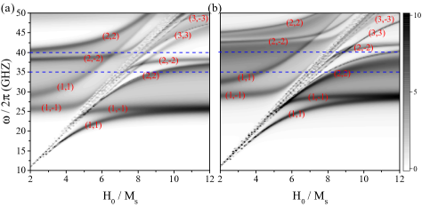
Figure 5: (Color online) Scattering efficiency factor $Q_{sca}$ as function of normalized magnetic field $H_{0}/M_{s}$ and frequency $\omega/2\pi$ for a YIG sphere of radius $a=1.25\,\mathrm{mm}$ and relative permittivity $\epsilon/\epsilon_{0}=15$ (a) in the center of a spherical cavity of radius $R=1.6\,\mathrm{mm}$ and (b) in the absence of the cavity. Dashed lines indicate the frequency range in Figure 4.

Our results help to interpret recent experimental results on YIG spheres in microwave cavities with reported coupling strength that are comparable with the magnon frequency Zhang2014 , i.e., in the ultrastrong-coupling regime. In Fig. 4 the scattering efficiency factor is shown as a function of $H_{0}/M_{s}$ and $\omega/2\pi$. Panel (a) addresses a YIG sphere of radii $a=1.25\,\mathrm{mm}$ in a spherical microwave cavity of radii $R=1.6\,\mathrm{mm}$, chosen to be close to the leading dimensions of the cavity in the experiments. Panel (b) holds for the same YIG sphere but without cavity. The obvious anticrossing in Fig. 4(a) is a signature of the emergence of the hybrid excitation that we refer to as magnon-polariton. The anti-crossing modes are labeled by the mode numbers $(n,m)$. For given $n$ there are two $m=\pm n$ anti-crossing modes with coupling strengths $g_{n,n}>g_{n,-n}$, where $g_{n,m}$ is the effective coupling strength of the magnon mode $(n,m)$ to the cavity. Fig. 4(a) indicates that the ultrastrong-coupling strength is indeed approached since a splitting of $g/2\pi=2.5\leavevmode\nobreak\$ GHz is achieved at a resonance frequency of $\omega/2\pi\simeq 37.5\,$ GHz. Beside the main anticrossing with the $(2,2)$ and $(2,-2)$ cavity modes, we observe tails from other anticrossings with the $(3,3)$ and $(3,-3)$ modes at higher frequencies, as well as the $(1,1)$ and $(1,-1)$ modes at lower frequencies, which are standing electromagnetic resonance modes confined by the YIG sphere. We may interpret these as nearly pure spin wave modes that acquire some oscillator strengths by mixing from far away resonances due to the ultrastrong coupling with standing microwaves. This can be verified by checking the scattering efficiency factor in the absence of the cavity as in Fig. 4(b), which emphasizes the antenna action of the YIG sphere.

Zhang et al. Zhang2014 indeed report additional, weakly-coupled “higher modes,”but without explaining their nature. They report ultrastrong-coupling between magnons and the cavity photons only in the frequency range of $35-40$ GHz, but data at lower frequencies are not given. In Fig. 5 we extend the plots in Fig. 4 to a larger frequency interval. We observe that the main anticrossing in the frequency range of $35-40$ GHz is caused by the $n=2$ modes, while hybridized modes originating from the $n=1$ resonance exist at the lower frequencies. The unperturbed modes between the anticrossing gaps are therefore not only due to the higher modes, but lower modes with ${n=1}$ also contribute by the ultrastrong-coupling. Two significant curves in the left and right side of the higher unperturbed modes originate from the anticrossing modes $n=1$ (the left one) and $n=2$ (the right one) of the YIG sphere itself, as is more clear in Fig. 5(b) (the computed lines are broader because we use a relatively large $\kappa$ for computational convenience). We thereby find again that the strong-coupling magnon-polariton may form also without cavity.

We concentrated on the dipolar spin wave excitations driven by magnetic fields that are strongly inhomogeneous due to a large dielectric constant. We disregard here exchange interactions, thereby limiting the validity of the treatment to YIG spheres much larger than the so-called exchange length that for YIG is only a few nanometers. In other words, we cannot properly describe all spin waves with relatively large wave number or frequencies relatively much higher relative to the FMR frequency. Indeed, in the planar configuration spin wave resonances are observable for rather thick films Cao . Exchange-induced whispering gallery modes on the surface of the YIG might therefore be observable even in thicker spheres, but their treatment is tedious and beyond the scope of the present paper.

IV Conclusion

In this paper we implement Mie scattering theory to study the interaction of dielectric as well as magnetic spheres with microwaves in cavities by the coupled LLG and Maxwell equations, disregarding only the exchange interaction. We are mainly interested in the coherent coupling between the magnons and microwave cavity modes in the strong- or even ultrastrong-coupling regimes characterized by the mode-dependent coupling strengths $g_{n,m}$. We reveal that while in the presence of a spherical cavity both strong and ultrastrong coupling can be realized by tuning the cavity modes and by increasing the filling factor of the cavity. Surprisingly, these regimes can also be achieved by removing the external resonator, due to the strong confinement of electromagnetic waves in sufficiently large YIG spheres. In this regime, higher angular momentum eigenmodes of the dielectric sphere participate and the scattering shows $s$- as well as $p$-wave character. We thereby transcend studies that focus on dipolar spin waves in a magnetostatic framework Walker ; Fletcher1959 by considering propagation effects via the full Maxwell equation. Our study might be useful in designing optimal conditions to design cavities in which YIG spheres are coherently coupled to, e.g., superconducting qubits, in microwave cavities for coherent quantum information transfer Tabuchi2014 .

- (1) A. Wallraff, D. I. Schuster, A. Blais, L. Frunzio, R.-S. Huang, J. Majer, S. Kumar, S. M. Girvin, and R. J. Schoelkopf, Nature 431, 162 (2004).
- (2) Y. Kubo, F. R. Ong, P. Bertet, D. Vion, V. Jacques, D. Zheng, A. Dréau, J. F. Roch, A. Auffeves, F. Jelezko, J. Wrachtrup, M. F. Barthe, P. Bergonzo, and D. Esteve, Phys. Rev. Lett. 105, 140502 (2010).
- (3) S. Putz, D. O. Krimer, R. Amsüss, A. Valookaran, T. Nöbauer, J. Schmiedmayer, S. Rotter and J. Majer, Nature Physics 10, 720 (2014).
- (4) N. Bar-Gill, L.M. Pham, A. Jarmola, D. Budker and R.L. Walsworth, Nature Communications 4, 1743 (2013).
- (5) L. Childress, M. V. Gurudev Dutt, J. M. Taylor, A. S. Zibrov, F. Jelezko, J. Wrachtrup, P. R. Hemmer and M. D. Lukin, Science 314, 281 (2006).
- (6) D. L. Mills and E. Burstein, Rep. Prog. Phys. 37 817 (1974).
- (7) A. Lehmeyer and L. Merten, J. Magn. Magn. Mater. 50, 32 (1985).
- (8) Y. Cao, P. Yan, H. Huebl, S.T.B. Goennenwein and G.E.W. Bauer, Phys. Rev. B. 91, 094423 (2015).
- (9) M. Tavis and F.W. Cummings, Phys. Rev. 170, 379 (1968).
- (10) J.M. Fink, R. Bianchetti, M. Baur, M. Göppl, L. Steffen, S. Filipp, P.J. Leek, A. Blais, and A. Wallraff, Phys. Rev. Lett. 103, 083601 (2009).
- (11) Spin Dynamics in Confined Magnetic Structures I, edited by B. Hillebrands and A. Thiaville (Springer-Verlag, Berlin, 2006).
- (12) C. Kittel, Phys. Rev. 110, 1295 (1958).
- (13) A. A. Serga, A. V. Chumak, and B. Hillebrands, J. Phys. D: Appl. Phys. 43, 264002 (2010).
- (14) M. Gilleo and S. Geller, Phys. Rev. 110, 73 (1958).
- (15) Y. Kajiwara, K. Harii, S. Takahashi, J. Ohe, K. Uchida, M. Mizuguchi, H. Umezawa, H. Kawai, K. Ando, K. Takanashi, S. Maekawa, and E. Saitoh, Nature 464, 262 (2010).
- (16) B. Heinrich, C. Burrowes, E. Montoya, B. Kardasz, E. Girt, Y.-Y. Song, Y. Sun, and M. Wu, Phys. Rev. Lett. 107, 066604 (2011).
- (17) H. Kurebayashi, O. Dzyapko, V.E. Demidov, D. Fang, A.J. Ferguson, and S.O. Demokritov, Nature Materials 10, 660 (2011).
- (18) H. Huebl, C.W. Zollitsch, J. Lotze, F. Hocke, M. Greifenstein, A. Marx, R. Gross, and S.T.B. Goennenwein, Phys. Rev. Lett. 111, 127003 (2013).
- (19) G.B.G. Stenning, G.J. Bowden, L.C. Maple, S.A. Gregory, A. Sposito, R.W. Eason, N.I. Zheludev, and P.A.J. de Groot, Opt. Exp. 21, 1456 (2013).
- (20) B. Bhoi, T. Cliff, I.S. Maksymov, M. Kostylev, R. Aiyar, N. Venkataramani, S. Prasad, and R.L. Stamps, J. Appl. Phys. 116, 243906 (2014).
- (21) Y. Tabuchi, S. Ishino, T. Ishikawa, R. Yamazaki, K. Usami, and Y. Nakamura, Phys. Rev. Lett. 113, 083603 (2014); Y. Tabuchi, S. Ishino, A. Noguchi, T. Ishikawa, R. Yamazaki, K. Usami, and Y. Nakamura, arXiv:1410.3781v1.
- (22) X. Zhang, C. Zou, L. Jiang, and H.X. Tang, Phys. Rev. Lett. 113, 156401 (2014).
- (23) M. Goryachev, W.G. Farr, D.L. Creedon, Y. Fan, M. Kostylev, and M.E. Tobar, Phys. Rev. Applied, 2, 054002 (2014).
- (24) D. Ballester, G. Romero, J. J. García-Ripoll, F. Deppe, and E. Solano, Phys. Rev. X 2, 021007, (2012).
- (25) A. Moroz, Annals of Physics 340, 252 (2014).
- (26) T. Niemczyk et al., Nature Physics 6, 772 (2010).
- (27) J. Casanova, G. Romero, I. Lizuain, J.J. García-Ripoll, and E. Solano, Phys. Rev. Lett. 105 263603 (2010).
- (28) Ivan S. Maksymov, Jessica Hutomo, Donghee Nam and Mikhail Kostylev, J. Appl. Phys. 117, 193909 (2015).
- (29) O. O. Soykal and M. E. Flatté, Phys. Rev. Lett. 104, 077202 (2010); Phys. Rev. B 82, 104413 (2010).
- (30) L. R. Walker, J. Appl. Phys. 29, 318 (1958).
- (31) P.C. Fletcher and R.O. Bell, J. Appl. Phys., 30, 687 (1959).
- (32) R. Arias, P. Chu, and D. Mills, Phys. Rev. B 71, 224410 (2005).
- (33) Mie, G., Ann. Phys., 330: 377 E45 (1908).
- (34) M. Kerker, "The scattering of light, and other electromagnetic radiation" Academic Press (1969).
- (35) J. A. Stratton, "Electromagnetic Theory" Wiley-IEEE Press (2007).
- (36) T.J. Gerson and J.S. Nadan, IEEE Trans. Microw. Theory Techn. 22, 757 (1974).
- (37) Z. Lin, and S. T. Chui, Phys. Rev. E 69, 056614 (2004).
- (38) J. Le-Wei Li, Wee-Ling Ong, and K. H. R. Zheng, Phys. Rev. E 85, 036601 (2012).
- (39) Andreasen, M.G., Antennas and Propagation, IRE Transactions, 5, 267 (1957).
- (40) Andreasen, M.G., Antennas and Propagation, IRE Transactions, 5, 337 (1957).
- (41) S. A. Manuilov, S. I. Khartsev, and A. M. Grishin, J. Appl. Phys. 106, 123917 (2009).
- (42) K. Sadhana, R. S. Shinde, and S. R. Murthy, Int. J. Mod. Phys. B 23, 3637 (2009).
- (43) http://deltroniccrystalindustries.com/deltronic_crystal_products/yttrium_iron_garnet
- (44) Dmitry S. Filonov, Alexander E. Krasnok, Alexey P. Slobozhanyuk, Polina V. Kapitanova, Elizaveta A. Nenasheva, Yuri S. Kivshar and Pavel A. Belov, Appl. Phys. Lett. 100, 201113 (2012).
- (45) Arseniy I. Kuznetsov, Andrey E. Miroshnichenko, Yuan Hsing Fu, JingBo Zhang and Boris Luk’yanchuk, Sci. Rep. 2, 492 (2012).
- (46) Guillaume Boudarham, Redha Abdeddaim and Nicolas Bonod, Appl. Phys. Lett. 104, 021117 (2014).
- (47) Ke Bi, Yunsheng Guo, Xiaoming Liu, Qian Zhao, Jinghua Xiao, Ming Lei and Ji Zhou, Sci. Rep. 4, 7001 (2014).
- (48) Andrey A. Nikitin, Alexey B. Ustinov, Alexander A. Semenov, Boris A. Kalinikos and E. Lähderanta, Appl. Phys. Lett. 104, 093513 (2014).