Quantum information processing on nitrogen-vacancy ensembles with the local resonance assisted by circuit QED

Abstract

With the local resonant interaction between a nitrogen-vacancy-center ensemble (NVE) and a superconducting coplanar resonator, and the single-qubit operation, we propose two protocols for the state transfer between two remote NVEs and for fast controlled-phase (c-phase) on these NVEs, respectively. This hybrid quantum system is composed of two distant NVEs coupled to separated high-$Q$ transmission line resonators (TLRs), which are interconnected by a current-biased Josephson-junction superconducting phase qubit. The fidelity of our state-transfer protocol is about $99.65\%$ within the operation time of $70.60$ ns. The fidelity of our c-phase gate is about $98.23\%$ within the operation time of $93.87$ ns. Furthermore, using the c-phase gate, we construct a two-dimensional cluster state on NVEs in $n\times n$ square grid based on the hybrid quantum system for the one-way quantum computation. Our protocol may be more robust, compared with the one based on the superconducting resonators, due to the long coherence time of NVEs at room temperature.

I Introduction

Universal quantum logic gates Sleator ; Nielsen1 are the key element for a quantum computer. In recent decades, much attention has been focused on the construction of universal quantum logic gates with different physical systems, such as ion trap Cirac1 ; Poyatos , cavity quantum electrodynamics (QED) cavity1 ; cavity2 ; fidlifuli , nuclear magnetic resonance NMRJones ; NMRLong , quantum dots Loss ; electron1 ; dotweisr ; dothybrid , photons with one degree of freedom (DOF) photon1 ; photon2 or two DOFs (that is, the hyper-parallel photonic quantum computation) hypercnotlpl ; hypercnotsr ; hypercnotPRA , superconducting qubit Makhlin2 ; Yang4 ; SQ1 ; SQ2 ; AiSQ , circuit QED circuitQED1 ; circuitQED2 ; circuitQED3 ; circuitQED4 ; circuitQED5 ; circuitQED6 ; circuitQED7 , microwave-photon resonators mwphoton ; Hua ; HuaSR , and diamond nitrogen-vacancy (NV) centers NVQC1 ; NVQC2 . Among the above schemes, much attention has been paid to the generation of the controlled-phase (c-phase) gate which can be used to realize universal quantum computation assisted with single-qubit operations.

In order to realize scalable quantum computation, tunable coupling and coherence time are of special importance. In this regard, each quantum system has its own advantages and disadvantages, e.g., easy operability but not enough long coherence time and thus insufficiently high fidelity. In order to overcome the disadvantages of each system to realize universal quantum computation, a hybrid quantum system Xiang , which is composed of two or more kinds of quantum systems, has attracted much attention recently.

The hybrid systems composed of superconducting circuits and the other quantum systems Xiang , such as atoms rensen ; Deng , molecules Rabl ; Tordrup1 , spins Imamo ; Chen1 ; Bushev , and solid-state devices Zhang1 ; You1 , have been studied. As a result of long coherence time of the NV-center spin Jelezko and the strong coupling between nitrogen-vacancy-center ensemble (NVE) and superconducting resonator Kubo1 ; Ams ; Sandner , the hybrid system composed of diamond NVE and superconducting circuit plays a good platform for quantum information processing. Recently, a lot of theoretical and experimental works have been done in the quantum information processing based on the hybrid system Kubo1 ; Sandner ; Kubo2 ; Yang2 ; Yang1 . For example, in 2010, Kubo and coworkers Kubo1 realized the strong coupling of a spin ensemble, which is composed of NV-centers in a diamond crystal, to a superconducting resonator. In 2012, Sandner et al. Sandner showed that a dense NVE can be coupled to a high-Q superconducting resonator at low temperature both in experiment and in theory. In 2011, Kubo et al. Kubo2 reported the experimental realization of a hybrid quantum circuit combining a superconducting transmon qubit and an NVE. Yang et al. Yang1 studied the high-fidelity quantum memory in a hybrid quantum computing system composed of an NVE and a current-biased Josephson-junction superconducting phase qubit in a transmission line resonator (TLR) (as the quantum data bus). They also Yang2 presented a potentially practical proposal for creating entanglement of two distant NVEs coupled to separated TLRs interconnected by a current-biased Josephson-junction superconducting phase qubit. In 2012, Chen, Yang, and Feng fengmang proposed a scheme for the state transfer between distant NVEs coupled with a superconducting flux qubit each, by modulating the coupling strength between flux qubits and that between a flux qubit and an NVE.

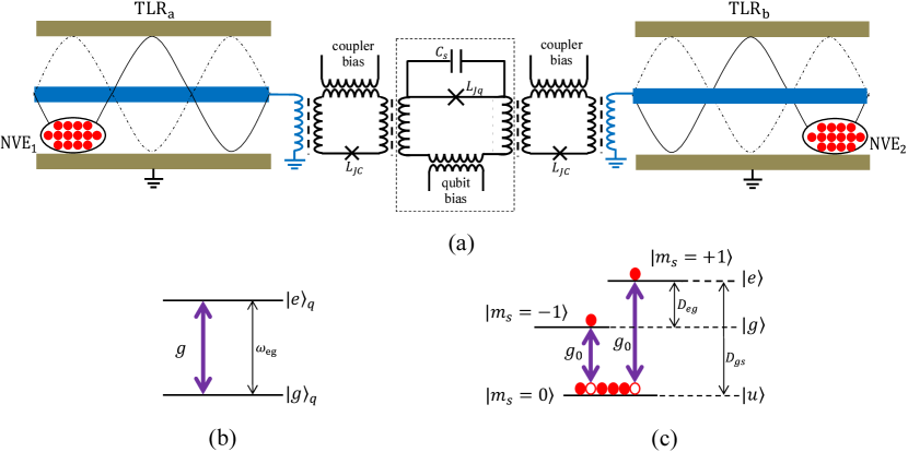
Figure 1: (Color online) (a) Schematic diagram of the hybrid quantum system for our quantum information processing on two NVEs. The TLRs are connected to the SPQ by two couplers. The coupling strength between the TLR and the SPQ can be tuned by the coupler. The NVEs interact with the quantized fields of TLRs, which act as a quantum data bus. (b) Level scheme of an SPQ. The SPQ is approximated as a two-level system and there is a large energy gap $\omega_{eg}$ between the two levels $|e\rangle_{q}$ and $|g\rangle_{q}$. (c) The detailed energy configuration of a single NV-center under an external magnetic field $\vec{B}$. The energy level difference between $|m_{s}=\pm 1\rangle$ is $D_{eg}=\gamma_{e}B$, where $\gamma_{e}$ is the electron gyromagnetic ratio. And the transition frequency between $|m_{s}=0\rangle$ and $|m_{s}=-1\rangle$ is $D_{gs}-D_{eg}$.

In this paper, we consider quantum information processing in a hybrid system composed of two distant NVEs coupled to separated high-$Q$ TLRs, which are interconnected by a current-biased Josephson-junction superconducting phase qubit (SPQ). By using the resonant interaction between the resonator and the NVE with the transition of $|m_{s}=0\rangle\leftrightarrow|m_{s}=-1\rangle$, and the single-qubit operation, we propose a protocol for the quantum state transfer between the two distant NVEs, and construct the c-phase and CNOT gates on these NVEs as well. Because both the resonant interaction between the NVE and the resonator and the single-qubit rotation on NVEs are fast quantum manipulation, our state transfer and gates have the features of a high fidelity and a short operation time. The fidelity of our state tranfer and c-phase gate are about $99.65\%$ and $98.23\%$, respectively. And the operation times of them are $70.60$ ns and $93.87$ ns, respectively. Furthermore, we construct a two-dimensional $n\times n$ squared grid based on the hybrid quantum system interconnected by the SPQs. Thus, by virtue of the long coherence time of NVE Yang2 ; Neumman , we engineer a cluster state of two-dimensional network for the one-way quantum computation with the promising advantage compared with the one based on the superconducting resonators Wu .

II Model and Quantum Dynamics Of System

Let us consider a hybrid quantum device composed of two distant NVEs coupled to separated high-$Q$ TLRs as shown in Fig. 1(a). The two TLRs are interconnected by an SPQ. The TLR with inductance $L$ and capacitance $C$ can be modeled as a simple harmonic oscillator circuitQED1 ; circuitQED3 consisting of a narrow center conductor and two nearby lateral ground planes Yang1 ; Yang2 . The Hamiltonians of TLR_a and TLR_b can be formed as

$$H_{a} = \omega_{a}a^{{\dagger}}a$$ (1)

and

$$H_{b} = \omega_{b}b^{{\dagger}}b,$$ (2)

respectively, where $a^{{\dagger}}$ ($\omega_{a}=1/\sqrt{LC}$) and $b^{{\dagger}}$ ($\omega_{b}=1/\sqrt{LC}$) are the creation operators (transition frequencies) of TLR_a and TLR_b, respectively.

The circuit in the dashed-line box of Fig. 1(a) is an SPQ. With the lowest two energy levels of an SPQ, the Hamiltonian is

$$H_{q}=\frac{1}{2}\omega_{eg}\sigma_{z}.$$ (3)

Here $\omega_{eg}$ is the resonant transition frequency between the two levels of the SPQ (see Fig. 1(b)), which can be changed by the external flux bias to the qubit Makhlin2 ; Galiautdinov . $\sigma_{z}=|e\rangle\langle e|-|g\rangle\langle g|$ is the Pauli spin operator of the SPQ, where $|g\rangle$ and $|e\rangle$ are the ground and excited states, respectively. By means of couplers, two TLRs are indirectly coupled to the SPQ and the coupling strength can be changed by applying different flux to the coupler Allman .

Taking the rotating-wave approximation into account, the interaction Hamiltonians between TLRs and SPQ are

$$H_{aq} = g_{a}(a\sigma^{+}+a^{{\dagger}}\sigma^{-}),$$ (4)

and

$$H_{bq} = g_{b}(b\sigma^{+}+b^{{\dagger}}\sigma^{-}),$$ (5)

respectively. Here, $g_{a}=(g_{b}=)g$ is the coupling strength between TLR_a (TLR_b) and SPQ. $\sigma^{+}=|e\rangle\langle g|$ $(\sigma^{-}=|g\rangle\langle e|)$ is the raising (lowering) operator of the SPQ.

NV-centers in the device possess a V-type three-energy-level configuration as shown in Fig. 1(c). Every NV-center is negatively charged with two unpaired electrons located at the vacancy. Thus, the spin-spin interaction leads to the same energy splitting between $|m_{s}=0\rangle$ and $|m_{s}=\pm 1\rangle$, i.e., $D_{gs}=2.88$ GHz Hanson . When there is an external magnetic field $\vec{B}$ along the NV-center symmetry axis, the degeneracy of the levels $|m_{s}=\pm 1\rangle$ is lifted, which causes a level splitting $D_{eg}=\gamma_{e}B$, with $\gamma_{e}$ being the gyromagnetic ratio of electron Chen1 . For simplicity, we label the states of the NV-center $|m_{s}=0\rangle,|m_{s}=-1\rangle$, and $|m_{s}=1\rangle$ as $|u\rangle,|g\rangle$, and $|e\rangle$, respectively. Moreover, the lowest level $|u\rangle$ of the NV-center is an auxiliary state in the present work. There are $N$ NV-centers in the single NVE and the Hamiltonian of an NVE reads

$$H_{k}=\frac{1}{2}\omega_{k,0}S_{k,0}^{z}+\frac{1}{2}\omega_{k,1}S_{k,1}^{z},$$ (6)

where $k=1,2$ are on behalf of NVE₁ and NVE₂. $\omega_{k,0}=D_{gs}-\gamma_{e}B_{k}$ and $\omega_{1,1}=\omega_{2,1}=D_{gs}$ are the transition frequencies of $|u\rangle\leftrightarrow|g\rangle$ and $|u\rangle\leftrightarrow|e\rangle$, respectively. $S_{k,0}^{z}=\sum_{i=1}^{N}\tau_{k,i}^{z}$ and $S_{k,0}^{\pm}=\sum_{i=1}^{N}\tau_{k,i}^{\pm}/\sqrt{N}$ are a set of collective spin operators Song ; Ai2 for NVE $k$ with $\tau_{k,i}^{z}=|g\rangle_{k,i}\langle g|-|u\rangle_{k,i}\langle u|$, $\tau_{k,i}^{+}=|g\rangle_{k,i}\langle u|$, and $\tau_{k,i}^{-}=|u\rangle_{k,i}\langle g|$. And $S_{k,1}^{z}=\sum_{i=1}^{N}v_{k,i}^{z}$ and $S_{k,1}^{\pm}=\sum_{i=1}^{N}v_{k,i}^{\pm}/\sqrt{N}$ are the other set of collective spin operators for NVE $k$ with $\upsilon_{k,i}^{z}=|e\rangle_{k,i}\langle e|-|u\rangle_{k,i}\langle u|$, $\upsilon_{k,i}^{+}=|e\rangle_{k,i}\langle u|$, and $\upsilon_{i}^{-}=|u\rangle_{k,i}\langle e|$.

The NVE qubit in this work is encoded in the following $|0\rangle$ and $|1\rangle$ states

$$|0\rangle_{k} = S_{k,0}^{+}|U\rangle_{k}=\frac{1}{\sqrt{N}}\sum_{i=1}^{N}|u_{1}\cdots g_{i}\cdots u_{N}\rangle_{k},$$ (7)

$$|1\rangle_{k} = S_{k,1}^{+}|U\rangle_{k}=\frac{1}{\sqrt{N}}\sum_{i=1}^{N}|u_{1}\cdots e_{i}\cdots u_{N}\rangle_{k},$$ (8)

where $|U\rangle_{k}=|u_{1}\cdots u_{i}\cdots u_{N}\rangle_{k}$ is the auxiliary state for an NVE. Using the rotating-wave approximation, the interaction Hamiltonian of an NVE coupled to the corresponding TLR by the magnetic-dipole coupling reads Yang2

$$H_{a1} = g_{1}(S_{1,0}^{+}a+S_{1,0}^{-}a^{{\dagger}}+S_{1,1}^{+}a+S_{1,1}^{-}a^{{\dagger}}),$$ (9)

and

$$H_{b2} = g_{2}(S_{2,0}^{+}b+S_{2,0}^{-}b^{{\dagger}}+S_{2,1}^{+}b+S_{2,1}^{-}b^{{\dagger}}),$$ (10)

where $g_{1}=\sqrt{N}g_{0}$, $g_{2}=\sqrt{N}g_{0}$, and $g_{0}$ is the single NV-center vacuum Rabi frequency. When the NVE is placed near the field antinode, the spatial dimension of the ensemble is smaller than the mode wavelength so that the spins in the NVE interact quasi-homogeneously with a single mode electromagnetic field.

The total Hamiltonian of our hybrid device composed of two NVEs coupled to separated TLRs interconnected by an SPQ can be described as

$$H=H_{a}+H_{b}+H_{q}+H_{1}+H_{2}+H_{aq}+H_{bq}+H_{a1}+H_{b2}.$$ (11)

In the interaction picture, by assuming $\omega_{a}=\omega_{eg}=\omega_{b}$, the total Hamiltonian becomes

$$H_{I}\!\!\! = \!\!\!g(a^{{\dagger}}\sigma^{-}+b^{{\dagger}}\sigma^{-})+g_{1}(a^{{\dagger}}S_{1,0}^{-}e^{-i\delta_{1,0}t}+a^{{\dagger}}S_{1,1}^{-}e^{-i\Delta t})$$ (12)

$$+g_{2}(b^{{\dagger}}S_{2,0}^{-}e^{-i\delta_{2,0}t}+b^{{\dagger}}S_{2,1}^{-}e^{-i\Delta t})+\textrm{h.c.}$$

Here, $\delta_{1,0}=\omega_{1,0}-\omega_{a}$, $\delta_{2,0}=\omega_{2,0}-\omega_{b}$, and $\Delta=\omega_{1,1}-\omega_{a}=\omega_{2,1}-\omega_{b}$.

Table 1: Scheme for the quantum state transfer between two NVEs.

Step	Transition	Coupling	Pulse
1) Rotate NVE1	$|1\rangle_{1}\rightarrow|U\rangle_{1}$	$\Omega_{R}/2$	$\pi$
2) Resonate	$|0\rangle_{1}|0\rangle_{a}\rightarrow|U\rangle_{1}|1\rangle_{a}$	$g_{1}$	$\pi$
3) Resonate	$|1\rangle_{a}|g\rangle_{q}|0\rangle_{b}\rightarrow|0\rangle_{a}|g\rangle_{q}|1\rangle_{b}$	$g$	$\sqrt{2}\pi$
4) Resonate	$|1\rangle_{b}|U\rangle_{2}\leftrightarrow|0\rangle_{b}|0\rangle_{2}$	$g_{2}$	$\pi$
5) Rotate NVE2	$|U\rangle_{2}\rightarrow|1\rangle_{2}$	$\Omega_{R}/2$	$3\pi$

III Quantum State Transfer between NVEs

In quantum information processing, the transfer of the quantum state from one location to another is an important task and it is the premise of the realization of large-scale quantum computing and quantum networks. Our device for the state transfer between distant NVEs is shown in Fig. 1(a) and this task can be achieved with five steps shown in Table 1. Its principle can be described in detail as follows.

Suppose that the hybrid quantum system composed of two NVEs, two TLRs, and the SPQ for the state transfer is initially in the superposition state

$$|\phi\rangle_{I}=(\alpha|0\rangle_{1}+\beta|1\rangle_{1})|0\rangle_{a}|g\rangle_{q}|0\rangle_{b}|U\rangle_{2},$$ (13)

where $\alpha$ and $\beta$ are complex numbers. $|n\rangle_{a}$ and $|n\rangle_{b}$ indicate the Fock states of TLR_a and TLR_b, respectively.

                    

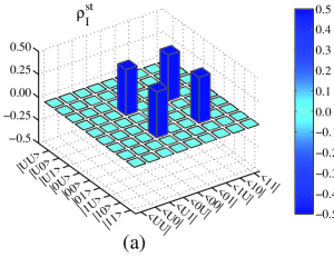
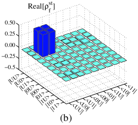
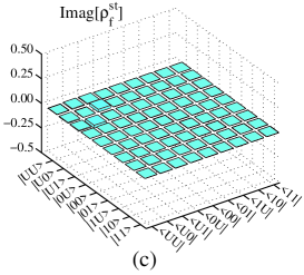
Figure 2: (Color online) (a) The density matrix of the initial state $\rho_{I}^{\text{st}}=\textrm{Tr}_{a,q,b}(|\phi\rangle_{I}\langle\phi|)$ (with $\alpha=\beta=1/\sqrt{2}$) of the system. (b) the real and (c) imaginary parts of the density matrix $\rho_{f}^{\text{st}}$ after the implementation of the state transfer, respectively.

In step (1), we apply an external drive field governed by $H_{D}^{\phi}=\Omega_{R}\exp(-i\omega_{d}t)S_{1,1}^{+}+\textrm{h.c.}$ with the Rabi frequency $\Omega_{R}$ and $\omega_{d}=\omega_{1,1}$ to flip the two states $|1\rangle_{1}\leftrightarrow|U\rangle_{1}$ of NVE₁. With the drive field, the Hamiltonian of the subsystem composed of NVE₁ and TLR_a is

$$H_{s1}^{\prime\phi}=H_{a}+H_{1}+H_{a1}+H_{D}^{\phi}.$$ (14)

In the interaction picture, the Hamiltonian reads

$$H_{s1}^{\phi}=g_{1}(a^{{\dagger}}S^{-}_{1,0}e^{-i\delta_{1,0}t}+a^{{\dagger}}S^{-}_{1,1}e^{-i\Delta t})+\frac{\Omega_{R}}{2}S_{1,1}^{+}+\textrm{h.c.}$$ (15)

In the large-detuning regime $\delta_{1,0},\Delta\gg g_{1}$, under the rotating-wave approximation, the Hamiltonian reads

$$H_{s1}^{\phi}\approx\frac{\Omega_{R}}{2}(S_{1,1}^{+}+S_{1,1}^{-}).$$ (16)

When the drive field is applied on the NVE₁ for a duration $t=\pi/\Omega_{R}$, the evolution of NVE₁ follows

$$|1\rangle_{1}\rightarrow-i|U\rangle_{1},$$ (17)

while the states of TLR_b and SPQ remain unaltered. That is, the evolution of the state of the system is

$$|\phi\rangle_{I}\;\rightarrow\;|\phi\rangle_{1}\!\!\! = \!\!\!(\alpha|0\rangle_{1}-i\beta|U\rangle_{1})|0\rangle_{a}|g\rangle_{q}|0\rangle_{b}|U\rangle_{2}.\;\;\;\;\;\;$$ (18)

In step (2), we tune the transition $|0\rangle_{1}\leftrightarrow|U\rangle_{1}$ of NVE₁ to achieve its local resonance with TLR_a by adjusting the applied magnetic field $\vec{B_{1}}$, and turn down the interaction between the SPQ and two TLRs by decreasing the coupling strength $g$ to $0.5$ MHz $\ll\min(g_{1}=16$ MHZ, $g_{2}=20$ MHz) Allman . Due to the weak coupling strength between the SPQ and TLRs, the energy transfer between the SPQ and TLRs can be omitted. The interaction Hamiltonian of the subsystem composed of NVE₁ and TLR_a is given by

$$H_{2}^{\phi}=g_{1}(a^{{\dagger}}S_{1,0}^{-}+a^{{\dagger}}S_{1,1}^{-}e^{-i\Delta t}+\textrm{h.c.}).$$ (19)

In the large-detuning regime $\Delta\gg g_{1}$, we can ignore the fast-oscillating terms, and the subsystem Hamiltonian can be simplified as

$$H_{2}^{\phi}\approx g_{1}(a^{{\dagger}}S_{1,0}^{-}+aS_{1,0}^{+}).$$ (20)

The evolution operator of this resonant interaction is written as $U_{2}(t)=\exp(-iH_{2}t)$. After a duration $t=\pi/2g_{1}$, we can obtain

$$|0\rangle_{1}|0\rangle_{a}\rightarrow-i|U\rangle_{1}|1\rangle_{a}.$$ (21)

After this local resonance, the state of the total system becomes

$$|\phi\rangle_{2}\!\!\! = \!\!\!|U\rangle_{1}(-i\alpha|1\rangle_{a}-i\beta|0\rangle_{a})|g\rangle_{q}|0\rangle_{b}|U\rangle_{2}.$$ (22)

In step (3), we turn up the coupling between the SPQ and TLRs by increasing the coupling strength $g$ to $104$ MHz Allman . And we can tune the transition frequencies of NVEs to be largely detuned with TLRs. In this case, there is only the energy transfer between the TLRs and the SPQ. The corresponding effective Hamiltonian is

$$H_{3}^{\phi}=g(a^{{\dagger}}\sigma^{-}+b^{{\dagger}}\sigma^{-}+\textrm{h.c.}).$$ (23)

Governed by this Hamiltonian with the duration $t=\pi/\sqrt{2}g$, the system evolves from the state $|\phi\rangle_{2}$ to

$$|\phi\rangle_{3}\!\!\! = \!\!\!|U\rangle_{1}|0\rangle_{a}|g\rangle_{q}(i\alpha|1\rangle_{b}-i\beta|0\rangle_{b})|U\rangle_{2}.$$ (24)

In step (4), we tune the transition frequency $\omega_{2,0}$ between $|0\rangle_{2}$ and $|U\rangle_{2}$ of NVE₂ to be equal to the frequency $\omega_{b}$ of TLR_b by adjusting the external magnetic field $\vec{B_{2}}$, and turn down the interaction between TLRs and the SPQ by turning the coupling strength $g$ to be $0.5$ MHz Allman . Without considering the weak interaction terms, the effective Hamiltonian is given by

$$\begin{split}H_{4}^{\phi}&=g_{2}(b^{{\dagger}}S_{2,0}^{-}+\textrm{h.c.}).\end{split}$$ (25)

In this step, the state driven by this Hamiltonian with the interval $t=\pi/g_{2}$ becomes

$$|\phi\rangle_{4}\!\!\! = \!\!\!|U\rangle_{1}|0\rangle_{a}|g\rangle_{q}|0\rangle_{b}(\alpha|0\rangle_{2}-i\beta|U\rangle_{2}).$$ (26)

In the last step (5), we apply a drive pulse with the duration $t=3\pi/\Omega_{R}$ on NVE₂ to induce the transition between $|1\rangle_{2}$ and $|U\rangle_{2}$. Thus an overall quantum state transfer between NVE₁ and NVE₂ is implemented, leaving the TLR_a, TLR_b, and the SPQ unchanged in the vacuum and ground state, that is,

$$|\phi\rangle_{\textrm{F}}\!\!\! = \!\!\!|U\rangle_{1}|0\rangle_{a}|g\rangle_{q}|0\rangle_{b}(\alpha|0\rangle_{2}+\beta|1\rangle_{2}).$$ (27)

To show the feasibility of our proposal for the state transfer between NVE₁ and NVE₂, we simulate the dynamics of the system with the Hamiltonian shown in Eq. (12). In the simulations, we choose the parameters $\omega_{a}/2\pi=\omega_{eg}/2\pi=\omega_{b}/2\pi=1.3$ GHz, $\omega_{1,0}/2\pi=\omega_{2,0}/2\pi=1.73$ GHz for the large-detuning case, $\omega_{1,1}/2\pi=\omega_{2,1}/2\pi=2.88$ GHz, $g_{1}/2\pi=16$ MHz, $g_{2}/2\pi=20$ MHz, and $g/2\pi=104$ (0.5) MHz when we turn up (down) the couplings between the SPQ and TLRs. The Rabi frequency induced by the drive field is $\Omega_{R}/2\pi=50$ MHz. If $\alpha=\sin\theta$ and $\beta=\cos\theta$, the final (target) state is $|\phi\rangle_{F}=|U\rangle_{1}|0\rangle_{a}|g\rangle_{q}|0\rangle_{b}(\sin\theta|0\rangle_{2}+\cos\theta|1\rangle_{2})$. Here the average fidelity of our proposal for the quantum state transfer is defined as fidlifuli ; HuaSR

$$F_{\phi}=\frac{1}{2\pi}\int_{0}^{2\pi}\,{}_{F}\langle\phi|\rho_{f}^{\textrm{st}}|\phi\rangle_{F}d\theta,$$ (28)

where $\rho_{f}^{\textrm{st}}$ is the realistic density operator after our state-transfer operation on the initial state $\left|\phi\right\rangle_{I}$. Our simulation shows that the fidelity of our state-transfer protocol is $99.65\%$ within the operation time $70.60$ ns. Taking $\alpha=\beta=1/\sqrt{2}$ as an example, the density operators of the initial state and the final state are shown in Fig. 2. The density matrix is spanned in the basis $\{~{}|U\rangle_{1}|U\rangle_{2},~{}|U\rangle_{1}|0\rangle_{2},~{}|U\rangle_{1}|1\rangle_{2},~{}|0\rangle_{1}|U\rangle_{2},~{}|0\rangle_{1}|0\rangle_{2}$, $~{}|0\rangle_{1}|1\rangle_{2},~{}|1\rangle_{1}|U\rangle_{2},~{}|1\rangle_{1}|0\rangle_{2},~{}|1\rangle_{1}|1\rangle_{2}$}.

               

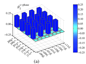
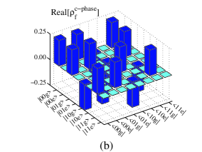
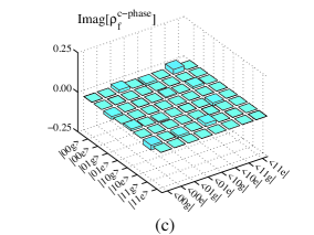
Figure 3: (Color online) (a) The density matrix of the initial state $\rho_{I}^{\text{c-phase}}=\textrm{Tr}_{a,q,b}(|\psi\rangle_{I}\langle\psi|)$ (with $\alpha=\beta=\gamma=\delta=1/2$) of the system. (b) the real and (c) imaginary parts of the density matrix $\rho_{f}^{\text{c-phase}}$ after the implementation of the c-phase gate, respectively.

IV C-phase and CNOT Gates on two NVEs

C-phase gate is one of the significant quantum logic gates for quantum information processing and it can be used to form a series of universal gates to achieve quantum computation Nielsen1 assisted by single-qubit operations. In the basis of two NVEs $\{|0\rangle_{1}|0\rangle_{2},|0\rangle_{1}|1\rangle_{1},|1\rangle_{1}|0\rangle_{2},|1\rangle_{1}|1\rangle_{2}\}$, the matrix of the c-phase gate reads

$$U_{\textrm{c-phase}}=\begin{pmatrix}1&0&0&0\\ 0&1&0&0\\ 0&0&-1&0\\ 0&0&0&1\end{pmatrix},$$

where there is a $\pi$ phase shift when the two-NVE system is in the state $|0\rangle_{1}|1\rangle_{2}$. The initial state of the hybrid quantum system composed of two NVEs, two TLRs, and an SPQ (the device is shown in Fig. 1(a)) is prepared as

$$|\psi\rangle_{I}\!\! = \!\!(\cos\theta_{1}|0\rangle_{1}+\sin\theta_{1}|1\rangle_{1})(\cos\theta_{2}|0\rangle_{2}+\sin\theta_{2}|1\rangle_{2})$$ (29)

$$\otimes|g\rangle_{q}|0\rangle_{a}|0\rangle_{b}$$

$$= \!\!(\alpha|0\rangle_{1}|0\rangle_{2}+\beta|0\rangle_{1}|1\rangle_{2}+\gamma|1\rangle_{1}|0\rangle_{2}+\delta|1\rangle_{1}|1\rangle_{2})\;\;\;\;$$

$$\otimes|g\rangle_{q}|0\rangle_{a}|0\rangle_{b},$$

where $\alpha=\cos\theta_{1}\cos\theta_{2}$, $\beta=\cos\theta_{1}\sin\theta_{2}$, $\gamma=\sin\theta_{1}\cos\theta_{2}$, and $\delta=\sin\theta_{1}\sin\theta_{2}$ are complex numbers. By combining the single-qubit flip on NVEs and the resonant interactions between NVEs and TLRs and those between TLRs and the SPQ, the c-phase gate on NVE₁ and NVE₂ can be achieved by five steps displayed in Table 2.

Table 2: Scheme for the c-phase gate between two NVEs.

Step	Transition	Coupling	Pulse
1) Resonate	$|0\rangle_{1}|0\rangle_{a}\rightarrow|U\rangle_{1}|1\rangle_{a}$	$g_{1}$	$\pi$
Rotate NVE2	$|0\rangle_{2}\rightarrow|U\rangle_{2}$	$\Omega_{R}/2$	$\pi$
2) Resonate	$|1\rangle_{a}|g\rangle_{q}|0\rangle_{b}\rightarrow|0\rangle_{a}|g\rangle_{q}|1\rangle_{b}$	$g$	$\sqrt{2}\pi$
3) Resonate	$|1\rangle_{b}|U\rangle_{2}\leftrightarrow|0\rangle_{b}|0\rangle_{2}$	$g_{2}$	$2\pi$
4) Resonate	$|0\rangle_{a}|g\rangle_{q}|1\rangle_{b}\rightarrow|1\rangle_{a}|g\rangle_{q}|0\rangle_{b}$	$g$	$\sqrt{2}\pi$
5) Resonate	$|U\rangle_{1}|1\rangle_{a}\rightarrow|1\rangle_{1}|0\rangle_{a}$	$g_{1}$	$3\pi$
Rotate NVE2	$|U\rangle_{2}\rightarrow|0\rangle_{2}$	$\Omega_{R}/2$	$\pi$

In step (1), we tune the transition $|0\rangle_{1}\leftrightarrow|U\rangle_{1}$ of NVE₁ to be resonant with TLR_a, which is similar to the second step in our state-transfer protocol. The effective Hamiltonian of the subsystem consisting of NVE₁ and TLR_a is $H_{s1}=H^{\phi}_{2}$. The subsystem evolves from $|0\rangle_{1}|0\rangle_{a}$ to the state $-i|U\rangle_{1}|1\rangle_{a}$ at the appropriate time $t=\pi/2g_{1}$, with other states unchanged through the evolution time.

Meanwhile, we apply a drive field described by $H_{D}=\Omega_{R}\exp(-i\omega_{2,0}t)S^{+}_{2,0}/2+\textrm{h.c.}$ with the Rabi frequency $\Omega_{R}$ and the frequency to be the transition frequency of $|0\rangle_{2}\leftrightarrow|U\rangle_{2}$. The Hamiltonian of the subsystem composed of NVE₂ and TLR_b is $H_{s2}^{\prime}=H_{b}+H_{2}+H_{b2}+H_{D}$. The Hamiltonian can be approximately reduced to be $H_{s2}\approx\frac{\Omega_{R}}{2}(S_{2,0}^{+}+S_{2,0}^{-})$. With the duration $t=\pi/\Omega_{R}$, the drive field applied on NVE₂ makes it evolve from $|0\rangle_{2}$ to $-i|U\rangle_{2}$, while the states of TLR_b and SPQ remain unaltered.

After step (1), the state of the total system becomes

$$|\psi\rangle_{1}\!\!\! = \!\!\!(-\alpha|U\rangle_{1}|U\rangle_{2}|1\rangle_{a}-i\beta|U\rangle_{1}|1\rangle_{2}|1\rangle_{a}-i\gamma|1\rangle_{1}|U\rangle_{2}|0\rangle_{a}$$ (30)

$$\!\!\!+\delta|1\rangle_{1}|1\rangle_{2}|0\rangle_{a})\otimes|g\rangle_{q}|0\rangle_{b}.$$

In step (2), we use the same method as that in the third step in our state-transfer protocol to achieve the state transfer from TLR_a to TLR_b. With the effective Hamiltonian $H_{e2}=H^{\phi}_{3}$ operating for the duration $t=\pi/\sqrt{2}g$, the system evolves from the state $|\psi\rangle_{1}$ to

$$|\psi\rangle_{2}\!\!\! = \!\!\!(\alpha|U\rangle_{1}|U\rangle_{2}|1\rangle_{b}+i\beta|U\rangle_{1}|1\rangle_{2}|1\rangle_{b}-i\gamma|1\rangle_{1}|U\rangle_{2}|0\rangle_{b}$$ (31)

$$+\delta|1\rangle_{1}|1\rangle_{2}|0\rangle_{b})\otimes|g\rangle_{q}|0\rangle_{a}.$$

In step (3), we exploit the Hamiltonian $H_{e3}=H_{4}^{\phi}$ to achieve the resonant interaction between TLR_b and the transition $|U\rangle_{2}\leftrightarrow|0\rangle_{2}$, similar to the fourth step in our state-transfer protocol. With the interval $t=\pi/g_{2}$, the state of the system becomes

$$|\psi\rangle_{3}\!\!\! = \!\!\!(-\alpha|U\rangle_{1}|U\rangle_{2}|1\rangle_{b}+i\beta|U\rangle_{1}|1\rangle_{2}|1\rangle_{b}-i\gamma|1\rangle_{1}|U\rangle_{2}|0\rangle_{b}$$ (32)

$$\!\!\!+\delta|1\rangle_{1}|1\rangle_{2}|0\rangle_{b})\otimes|g\rangle_{q}|0\rangle_{a}.$$

Step (4) is the same as step (2). By virtue of simultaneous resonant interactions between the SPQ and the two TLRs, we can obtain the state

$$|\psi\rangle_{4}\!\!\! = \!\!\!(\alpha|U\rangle_{1}|U\rangle_{2}|1\rangle_{a}-i\beta|U\rangle_{1}|1\rangle_{2}|1\rangle_{a}-i\gamma|1\rangle_{1}|U\rangle_{2}|0\rangle_{a}$$ (33)

$$\!\!\!+\delta|1\rangle_{1}|1\rangle_{2}|0\rangle_{a})\otimes|g\rangle_{q}|0\rangle_{b}.$$

The last step (5) is the same as step (1). A drive pulse with the duration $t=\pi/\Omega_{R}$ is applied to induce the transition between $|0\rangle_{2}$ and $|U\rangle_{2}$ of NVE₂. Meanwhile, a resonant interaction between NVE₁ and TLR_a lasts for $g_{1}t=3\pi/2$. Thus an overall c-phase gate between NVE₁ and NVE₂ is implemented, leaving the TLR_a, TLR_b and the SPQ in the vacuum and ground states, that is,

$$|\psi\rangle_{F}\! = \!(\alpha|0\rangle_{1}|0\rangle_{2}+\beta|0\rangle_{1}|1\rangle_{2}-\gamma|1\rangle_{1}|0\rangle_{2}+\delta|1\rangle_{1}|1\rangle_{2})\;\;\;\;$$ (34)

$$\otimes|g\rangle_{q}|0\rangle_{a}|0\rangle_{b}.$$

Our simulation on the dynamics of the system with the Hamiltonian in Eq. (12) shows that the average fidelity of our c-phase gate is $98.23\%$ within the operation time $93.87$ ns. Here the average fidelity is defined as

$$F_{\textrm{c-phase}}=(\frac{1}{2\pi})^{2}\int_{0}^{2\pi}\int_{0}^{2\pi}\,{}_{F}\langle\psi|\rho_{f}^{\textrm{c-phase}}|\psi\rangle_{F}d\theta_{1}d\theta_{2},$$

(35)

similar to that in Eq. (28). In our simulation, the parameters are chosen as $\omega_{a}/2\pi=\omega_{eg}/2\pi=\omega_{b}/2\pi=1.4$ GHz, $\omega_{1,0}/2\pi=\omega_{2,0}/2\pi=2.08$ GHz for the large-detuning case, $\omega_{1,1}/2\pi=\omega_{2,1}/2\pi=2.88$ GHz, $g_{1}/2\pi=16$ MHz, $g_{2}/2\pi=20$ MHz, and $\Omega_{R}/2\pi=50$ MHz. $g/2\pi=104$ (0.5) MHz when we turn up (down) the coupling between the SPQ and TLRs. As an example for the fidelity of our gate with $\theta_{1}=\theta_{2}=\pi/4$, the density operators of the initial state and the final state are shown in Fig. 3. Here, the density matrix is spanned in the basis $\{|0\rangle_{1}|0\rangle_{2}|g\rangle_{q},~{}|0\rangle_{1}|0\rangle_{2}|e\rangle_{q},~{}|0\rangle_{1}|1\rangle_{2}|g\rangle_{q},~{}|0\rangle_{1}|1\rangle_{2}|e\rangle_{q},$ $~{}|1\rangle_{1}|0\rangle_{2}|g\rangle_{q},~{}|1\rangle_{1}|0\rangle_{2}|e\rangle_{q},~{}|1\rangle_{1}|1\rangle_{2}|g\rangle_{q},~{}|1\rangle_{1}|1\rangle_{2}|e\rangle_{q}\}$.

Table 3: Protocol for realization of CNOT gate between NVE₁ and NVE₂.

Step	Transition	Coupling	Pulse
1) Resonate	$|0\rangle_{1}|0\rangle_{a}\rightarrow|U\rangle_{1}|1\rangle_{a}$	$g_{1}$	$\pi$
Rotate	$|0\rangle_{2}\rightarrow|U\rangle_{2}$	$\Omega_{R}/2$	$\pi$
2) Resonate	$|1\rangle_{a}|g\rangle_{q}|0\rangle_{b}\rightarrow|0\rangle_{a}|g\rangle_{q}|1\rangle_{b}$	$g$	$\sqrt{2}\pi$
3) Resonate	$|1\rangle_{b}|U\rangle_{2}\rightarrow|0\rangle_{b}|0\rangle_{2}$	$g_{2}$	$\pi$
4) Resonate	$|1\rangle_{2}\leftrightarrow|U\rangle_{2}$	$\Omega_{R}/2$	$\pi$
5) Resonate	$|1\rangle_{b}|U\rangle_{2}\rightarrow|0\rangle_{b}|0\rangle_{2}$	$g_{2}$	$\pi$
6) Resonate	$|1\rangle_{2}\leftrightarrow|U\rangle_{2}$	$\Omega_{R}/2$	$3\pi$
7) Resonate	$|0\rangle_{b}|0\rangle_{2}\rightarrow|1\rangle_{b}|U\rangle_{2}$	$g_{2}$	$\pi$
8) Resonate	$|0\rangle_{a}|g\rangle_{q}|b\rangle_{b}\rightarrow|1\rangle_{a}|g\rangle_{q}|0\rangle_{b}$	$g$	$\sqrt{2}\pi$
9) Resonate	$|U\rangle_{1}|1\rangle_{a}\rightarrow|0\rangle_{1}|0\rangle_{a}$	$g_{1}$	$\pi$
Rotate	$|U\rangle_{2}\rightarrow|0\rangle_{2}$	$\Omega_{R}/2$	$3\pi$

Local resonant interaction and single-qubit operations can also be used to construct the fast CNOT gate on NVEs in the hybrid device. The matrix of the CNOT gate reads

$$U_{\textrm{CNOT}}=\begin{pmatrix}0&1&0&0\\ 1&0&0&0\\ 0&0&1&0\\ 0&0&0&1\end{pmatrix}$$

in the computational two-NVEs basis, that is, $\{|0\rangle_{1}|0\rangle_{2},|0\rangle_{1}|1\rangle_{1},|1\rangle_{1}|0\rangle_{2},|1\rangle_{1}|1\rangle_{2}\}$. The nine steps for the construction of the CNOT gate on two NVEs are shown in Table 3. It can be implemented with the processes similar to those for our c-phase gate.

V GENERATION of CLUSTER STATE IN ONE-DIMENSIONAL and TWO-DIMENSIONAL CIRCUITS

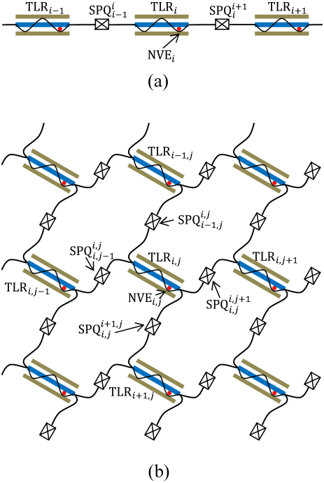
Figure 4: (Color online) The schematic layout of generating the large cluster state based on the 1D circuit chain (a) and the 2D square grid circuit (b). And the red dot embedded in the TLR represents an NVE.

Using the c-phase gate, one can construct a two-dimensional (2D) cluster state, which can be used to realize a one-way quantum computing Nielsen1 ; Wu ; Haack ; Raussendorf ; Nielsen2 . Before generating a 2D cluster state in a hybrid circuit grid, we try to implement a one-dimensional (1D) cluster state Nielsen2 in a hybrid circuit chain. Now, we will demonstrate in detail how to make use of the initial state $\prod^{\otimes n}_{i=1}(|0\rangle_{i}+|1\rangle_{i})/\sqrt{2}$ and our c-phase gate to generate the large NVE cluster state. In order to realize this initial state, we can apply two external drive fields to induce the transitions of $|U\rangle\leftrightarrow|0\rangle$ and $|U\rangle\leftrightarrow|1\rangle$. In the first step, as shown in Fig. 4(a), we divide the NVEs into many pairs NVE_2i-1—NVE_2i ($i=1,2,\cdots$) and tune the transition frequencies of $\textrm{SPQ}_{2i}^{2i+1}$ ($i=1,2,\cdots$) to the largely-detuned regime to form independent pairs in which each is a subsystem shown in Fig. 1(a). Then we operate c-phase gates between NVE_2i-1 and NVE_2i ($i=1,2,\cdots$). After this step, the state of the system composed of all the NVEs is

$$\frac{1}{2^{n}}\prod^{\otimes n}_{i=1}(|0\rangle_{2i-1}+\sigma_{2i}^{z}|1\rangle_{2i-1})(|0\rangle_{2i}+|1\rangle_{2i}),$$ (36)

where $\sigma_{2i}^{z}$ is the Pauli-Z operator for NVE_2i. In the second step, we perform the c-phase gate on NVE pairs $(2i,2i+1)$ ($i=1,2,\cdots$) as the same as that in the first step. Then we can prepare the chain in the cluster state

$$\frac{1}{\sqrt{2^{n}}}\prod^{\otimes n}_{i=1}(|0\rangle_{i}+\sigma_{i+1}^{z}|1\rangle_{i}),$$ (37)

where $\sigma_{n+1}^{z}\equiv 1$.

Now, we will demonstrate the four steps to generate a 2D cluster state in the $n\times n$ square grid Helmer as shown in Fig. 4(b). First of all, as in the 1D case, two sets of c-phase gates are sequentially performed to prepare the NVEs in each row into a 1D cluster state

$$\frac{1}{\sqrt{2^{n^{2}}}}\prod^{\otimes n}_{i,j=1}(|0\rangle_{i,j}+\sigma_{i,j+1}^{z}|1\rangle_{i,j}),$$ (38)

where $\sigma_{i,j+1}^{z}$ is the Pauli-Z operator for NVE_i,j+1. Second, the same operations are performed on the columns as on the rows. Then the 2D cluster state is

$$\frac{1}{\sqrt{2^{n^{2}}}}\prod^{\otimes n}_{i,j=1}(|0\rangle_{i,j}+\sigma_{i,j+1}^{z}\sigma_{i+1,j}^{z}|1\rangle_{i,j}),$$ (39)

where $\sigma_{i,n+1}^{z}\equiv\sigma_{n+1,j}^{z}\equiv 1$. In fact, this method can be extended to the general case, i.e., to prepare a $d$D cluster in which $2d$ steps are needed since in each dimension $2$ steps are required.

VI DISCUSSION AND SUMMARY

Recently, the hybrid quantum system made up of NVEs and superconducting circuits has been studied for quantum computation Kubo2 ; Yang1 ; Yang2 . In the system, the coupling strength between an NVE and a TLR can be enhanced to about $10\sim 65$ MHz Kubo1 ; Sandner , and the NVE can act as either a qubit or a good memory because the coherence time of an NV-center is much longer than that of an SPQ Jelezko .

In previous works about hybrid systems, the proposals for the entanglement or information transfer between two NVEs with the states $|m_{s}=0\rangle$ and $|m_{s}=\pm 1\rangle$ Yang1 ; Yang2 has been studied. To avoid the indirect interaction between the two NVEs, which can be induced by coupling with the same field mode, we place these two NVEs in two different TLRs. Moreover, because the two TLRs are connected by an SPQ with tunable couplings Allman ; Srinivasan , the induced interaction between the two NVEs can be effectively turned on and off. On the other hand, using the states $|m_{s}=0\rangle$ and $|m_{s}=1\rangle$ alone with the fixed level spacing leads to the difficulty in operation Helmer . In order to overcome this problem, we construct the fast universal quantum gate by using the computational states $|m_{s}=-1\rangle_{i}$ and $|m_{s}=+1\rangle_{i}$ in combination with the third auxiliary energy level $|m_{s}=0\rangle_{i}$, which gives us more freedom to achieve quantum information processing.

In 2012, in an interesting work by Chen et al. fengmang , the operation time of quantum state transfer, from the initial state $(\alpha|0\rangle_{\textrm{NVE}_{1}}+\beta|1\rangle_{\textrm{NVE}_{1}})|0\rangle_{\textrm{NVE}_{2}}$ to the final state $|0\rangle_{\textrm{NVE}_{1}}(\alpha|0\rangle_{\textrm{NVE}_{2}}-i\beta|1\rangle_{\textrm{NVE}_{2}})$, needs only $30$ ns with coupling strength between NVE and superconducting circuits about $70$ MHz. We remark that our proposal adopts a different final state with respect to theirs. If we choose the state transfer from $(\alpha|0\rangle_{\textrm{NVE}_{1}}+\beta|1\rangle_{\textrm{NVE}_{1}})|U\rangle_{\textrm{NVE}_{2}}$ to the same final state as theirs with the same coupling between NVE and superconducting circuits, the whole procedure in our proposal will reduce to four steps and the whole operation time is significantly reduced to $13.41$ ns with the fidelity about $96.88\%$. In addition, different from the proposal proposed by Yang et. al. Yang2 in 2012 for the state transfer between two NVEs within $400$ ns by using the global resonance on the whole hybrid system, our protocol for this task requires merely $70.60$ ns by using the local resonance between an NVE (the SPQ) and TLRs. Another advantage of the local resonance is that by virtue of the local resonance we can construct a multi-dimensional cluster state with only a few steps.

Resonance operation between an artificial atom and a cavity is one of the fast quantum operations. The resonance operation between an NVE and a superconducting resonator can be completed with a very high fidelity about 97% Yang1 . The resonance operation between an SPQ and a superconducting resonator can also be achieved with a very high fidelity, as shown in Refs. Haack ; You2 ; Sillanp . The coupling strength between the qubit and the resonator can be achieved as high as 100 MHz Allman , which suggests the quantum information transfer from resonator $a$ to resonator $b$ can be achieved within a very short time, compared to the decoherence time. The main factor which limits the operation time of our c-phase gate is the interaction between the NVE and the resonator. Since the couplings between NV-centers and resonator are quasi-homogeneous, the coupling strength between the collective mode and the resonator has been enhanced by $\sqrt{N}$ Song ; Ai2 . In our simulations, we do not consider the decoherence and leakage mechanisms of the hybrid system, due to the short operation time $93.87$ ns as compared to the coherence times of NV-center $\sim 10^{-3}$s Jelezko ; Choi and the SPQ $\sim 10^{-5}$s Xiang ; Yu , and the large quality factor of the superconducting resonator $>10^{6}$ Devoret ; Chen2 ; Leek ; Megrant . We remark that the quantum dynamics given by quantum master equation Breuer02 which takes decoherent effects into account and can be solved by quantum Monte Carlo approach Dalibard92 ; Piilo08 ; Ai14 ; Ai13 will be essentially very close to the present result. With the help of the short operation time of the c-phase gate, we can effectively construct the one-way quantum computation. Due to the long coherence time of the NVE, our one-way quantum computation based on the NVE has a longer life time than the effective scheme by Wu et al. Wu based on the 1D superconducting resonators.

In summary, we have proposed an effective scheme for the state transfer between two remote NVEs and that for the fast c-phase gate on them. Our hybrid system consists of two distant NVEs coupled to separated high-$Q$ TLRs, which are interconnected by an SPQ. The quantum state transfer and the c-phase gate are implemented by using local resonant interaction between the NVE and the resonator, and the single-qubit operation on the NVE, not global resonance Yang1 ; Yang2 . The fidelity of our quantum state transfer is $99.65\%$ within a short operation $70.60$ ns. The fidelity of our c-phase gate is $98.23\%$ within a short operation time of $93.87$ ns. Assisted by our c-phase gate, we propose a scheme to generate a two-dimensional cluster state on distinct NVEs in a square grid based on the above hybrid quantum system interconnected by the charge qubits. In this hybrid system, we can construct a one-way quantum computation with long coherent time in comparison with that based on the pure superconducting circuit system.

References

- (1) T. Sleator and H. Weinfurter, Phys. Rev. Lett. 74, 4087 (1995).
- (2) M. A. Nielsen and I. L. Chuang, Quantum Computing and Quantum Information (Cambridge University Press, Cambridge, UK, 2000).
- (3) J. I. Cirac and P. Zoller, Phys. Rev. Lett. 74, 4091 (1995).
- (4) J. F. Poyatos, J. I. Cirac, and P. Zoller, Phys. Rev. Lett. 81, 1322 (1998).
- (5) Q. A. Turchette, C. J. Hood, W. Lange, H. Mabuchi, and H. J. Kimble, Phys. Rev. Lett. 75, 4710 (1995).
- (6) A. Rauschenbeutel, G. Nogues, S. Osnaghi, P. Bertet, M. Brune, J. M. Raimond, and S. Haroche, Phys. Rev. Lett. 83, 5166 (1999).
- (7) Z. Q. Yin and F. L. Li, Phys. Rev. A 75, 012324 (2007).
- (8) J. A. Jones, M. Mosca, and R. H. Hansen, Nature (London) 393, 344 (1998).
- (9) G. Feng, G. Xu, and G. Long, Phys. Rev. Lett. 110, 190501 (2013).
- (10) D. Loss and D. P. DiVincenzo, Phys. Rev. A 57, 120 (1998).
- (11) X. Li, Y. Wu, D. Steel, D. Gammon, T. H. Stievater, D. S. Katzer, D. Oark, C. Piermarochi, and J. Sham, Science 301, 809 (2003).
- (12) H. R. Wei and F. G. Deng, Sci. Rep. 4, 7551 (2014).
- (13) H. R. Wei and F. G. Deng, Phys. Rev. A 87, 022305 (2013).
- (14) E. Knill, R. Laflamme, and G. J. Milburn, Nature (London) 409, 46 (2001).
- (15) K. Nemoto and W. J. Munro, Phys. Rev. Lett. 93, 250502 (2004).
- (16) B. C. Ren, H. R. Wei, and F. G. Deng, Laser Phys. Lett. 10, 095202 (2013).
- (17) B. C. Ren and F. G. Deng, Sci. Rep. 4, 4623 (2014).
- (18) B. C. Ren and F. G. Deng, arXiv:1411.0274.
- (19) Y. Makhlin, G. Scöhn, and A. Shnirman, Rev. Mod. Phys. 73, 357 (2001).
- (20) Y. Yamamoto, Y. A. Pashkin, O. Astafiev, Y. Nakamura, and J. S. Tsai, Nature (London) 425, 941 (2003).
- (21) C. P. Yang, Shih-I Chu, and S. Han, Phys. Rev. A 67, 042311 (2003).
- (22) Y. X. Liu, J. Q. You, L. F. Wei, C. P. Sun, and F. Nori, Phys. Rev. Lett. 95, 087001 (2005).
- (23) Q. Ai, W. Y. Huo, G. L. Long, and C. P. Sun, Phys. Rev. A 80, 024101 (2009).
- (24) A. Blais, R. S. Huang, A. Wallraff, S. M. Girvin, and R. J. Schoelkopf, Phys. Rev. A 69, 062320 (2004).
- (25) I. Chiorescu, P. Bertet, K. Semba, Y. Nakamura, C. J. P. M. Harmans, and J. E. Mooij, Nature (London) 431, 159 (2004).
- (26) A. Blais, J. Gambetta, A. Wallraff, D. I. Schuster, S. M. Girvin, M. H. Devoret, and R. J. Schoelkopf, Phys. Rev. A 75, 032329 (2007).
- (27) L. DiCarlo, J. M. Chow, J. M. Gambetta, Lev S. Bishop, B. R. Johnson, D. I. Schuster, J. Majer, A. Blais, L. Frunzio, S. M. Girvin, and R. J. Schoelkopf, Nature (Londin) 460, 240 (2009).
- (28) C. P. Yang, S. B. Zheng, and F. Nori, Phys. Rev. A 82, 062326 (2010).
- (29) Y. Cao, W. Y. Huo, Q. Ai, and G. L. Long, Phys. Rev. A 84, 053846 (2011).
- (30) C. P. Yang, Q. P. Su, and J. M. Liu, Phys. Rev. A 86, 024301 (2012).
- (31) F. W. Strauch, Phys. Rev. A 84, 052313 (2011).
- (32) M. Hua, M. J. Tao, and F. G. Deng, Phys. Rev. A 90, 012328 (2014).
- (33) M. Hua, M. J. Tao, and F. G. Deng, Sci. Rep. (in press); arXiv:1408.2168.
- (34) F. Jelezko, T. Gaebel, I. Popa, M. Domhan, A. Gruber, and J. Wrachtrup, Phys. Rev. Lett. 93, 130501 (2004).
- (35) H. R. Wei and F. G. Deng, Phys. Rev. A 88, 042323 (2013).
- (36) Z. L. Xiang, S. Ashhab, J. Q. You, and F. Nori, Rev. Mod. Phys. 85, 623 (2013).
- (37) A. S. Sørensen, C. H. van der Wal, L. I. Childress, and M. D. Lukin, Phys. Rev. Lett. 92, 063601 (2004).
- (38) Z. J. Deng, Q. Xie, C. W. Wu, and W. L. Yang, Phys. Rev. A 82, 034306 (2010).
- (39) P. Rabl, D. DeMille, J. M. Doyle, M. D. Lukin, R. J. Schoelkopf, and P. Zoller, Phys. Rev. Lett. 97, 033003 (2006).
- (40) K. Tordrup and K. Mølmer, Phys. Rev. A 77, 020301 (2008).
- (41) A. Imamoǧlu, Phys. Rev. Lett. 102, 083602 (2009).
- (42) P. Bushev, A. K. Feofanov, H. Rotzinger, I. Protopopov, J. H. Cole, C. M. Wilson, G. Fischer, A. Lukashenko, and A. V. Ustinov, Phys. Rev. B 84, 060501 (2011).
- (43) Q. Chen, W. L. Yang, M. Feng, and J. F. Du, Phys. Rev. A 83, 054305 (2011).
- (44) P. Zhang, Y. D. Wang, and C. P. Sun, Phys. Rev. Lett. 95, 097204 (2005).
- (45) J. Q. You, Y. X. Liu, and F. Nori, Phys. Rev. Lett. 100, 047001 (2008).
- (46) F. Jelezko, T. Gaebel, I. Popa, A. Gruber, and J. Wrachtrup, Phys. Rev. Lett. 92, 076401 (2004).
- (47) Y. Kubo, F. R. Ong, P. Bertet, D. Vion, V. Jacques, D. Zheng, A. Dréau, J. -F. Roch, A. Auffeves, F. Jelezko, J. Wrachtrup, M. F. Barthe, P. Bergonzo, and D. Esteve, Phys. Rev. Lett. 105, 140502 (2010).
- (48) R. Amsüss, Ch. Koller, T. Nöbauer, S. Putz, S. Rotter, K. Sandner, S. Schneider, M. Schramböck, G. Steinhauser, H. Ritsch, J. Schmiedmayer, and J. Majer, Phys. Rev. Lett. 107, 060502 (2011).
- (49) K. Sandner, H. Ritsch, R. Amsüss, Ch. Koller, T. Nöbauer, S. Putz, J. Schmiedmayer, and J. Majer, Phys. Rev. A 85, 053806 (2012).
- (50) Y. Kubo, C. Grezes, A. Dewes, T. Umeda, J. Isoya, H. Sumiya, N. Morishita, H. Abe, S. Onoda, T. Ohshima, V. Jacques, A. Dréau, J. -F. Roch, I. Diniz, A. Auffeves, D. Vion, D. Esteve, and P. Bertet, Phys. Rev. Lett. 107, 220501 (2011).
- (51) W. L. Yang, Z. Q. Yin, Y. Hu, M. Feng, and J. F. Du, Phys. Rev. A 84, 010301(R) (2011).
- (52) W. L. Yang, Y. Hu, Z. Q. Yin, Z. J. Deng, and M. Feng, Phys. Rev. A 83, 022302 (2011).
- (53) Q. Chen, W. L. Yang, and M. Feng, phys. Rev. A 86, 022327 (2012).
- (54) P. Neumann, N. Mizuochi, F. Rempp, P. Hemmer, H. Watanabe, S. Yamasaki, V. Jacques, T. Gaebel, F. Jelezko, and J. Wrachtrup, Science 320, 1326 (2008).
- (55) C. W. Wu, M. Gao, H. Y. Li, Z. J. Deng, H. Y. Dai, P. X. Chen, and C. Z. Li, Phys. Rev. A 85, 042301 (2012).
- (56) A. Galiautdinov, Phys. Rev. A 79, 042316 (2009).
- (57) M. S. Allman, F. Altomare, J. D. Whittaker, K. Cicak, D. Li, A. Sirois, J. Strong, J. D. Teufel, and R.W. Simmonds, Phys. Rev. Lett. 104, 177004 (2010).
- (58) R. Hanson, F. M. Mendoza, R. J. Epstein, and D. D. Awschalom, Phys. Rev. Lett. 97, 087601 (2006).
- (59) Z. Song, P. Zhang, T. Shi, and C. P. Sun, Phys. Rev. B 71, 205314 (2005).
- (60) Q. Ai, Y. Li, G. L. long, and C. P. Sun, Eur. Phys. J. D 48, 293 (2008).
- (61) G. Haack, F. Helmer, M. Mariantoni, F. Marquardt, and E. Solano, Phys. Rev. B 82, 024514 (2010).
- (62) R. Raussendorf and H. J. Briegel, Phys. Rev. Lett. 86, 5188 (2001).
- (63) M. A. Nielsen, Rep. Math. Phys. 57, 147 (2006).
- (64) F. Helmer, M. Mariantoni, A. G. Fowler, J. Delft, E. Solano, and F. Marquardt, Europhys. Lett. 85, 50007 (2009).
- (65) S. J. Srinivasan, A. J. Hoffman, J. M. Gambetta, and A. A. Houck, Phys. Rev. Lett. 106, 083601 (2011).
- (66) J. Q. You, J. S. Tsai, and F. Nori, Phys. Rev. B 68, 024510 (2003).
- (67) M. A. Sillanpää, J. I. Park, and R. W. Simmonds, Nature (London) 449, 438 (2007).
- (68) S. K. Choi, M. Jain, and S. G. Louie, Phys. Rev. B 86, 041202(R) (2012).
- (69) Y. Yu, S. Y. Han, X. Chu, S. I. Chu, and Z. Wang, Science 296, 889 (2002).
- (70) M. H. Devoret and R. J. Schoelkopf, Science 339, 1169 (2013).
- (71) W. Chen, D. A. Bennett, V. Patel, and J. E. Lukens, Supercond. Sci. Technol. 21, 075013 (2008).
- (72) P. J. Leek, M. Baur, J. M. Fink, R. Bianchetti, L. Steffen, S. Filipp, and A. Wallraff, Phys. Rev. Lett. 104, 100504 (2010).
- (73) A. Megrant, C. Neill, R. Barends, B. Chiaro, Y. Chen, L. Feigl, J. Kelly, E. Lucero, M. Mariantoni, P. J. J. O’Malley, D. Sank, A. Vainsencher, J. Wenner, T. C. White, Y. Yin, J. Zhao, C. J. Palmstrøm, J. M. Martinis, and A. N. Cleland, Appl. Phys. Lett. 100, 113510 (2012).
- (74) H. P. Breuer and F. Petruccione, The Theory of Open Quantum Systems (Oxford University Press, Oxford, 2002).
- (75) J. Dalibard, Y. Castin, and K. Mølmer, Phys. Rev. Lett. 68, 580 (1992).
- (76) J. Piilo, S. Maniscalco, K. Harkonen, and K. A. Suominen, Phys. Rev. Lett. 100, 180402 (2008).
- (77) Q. Ai, Y. J. Fan, B. Y. Jin, and Y. C. Cheng, New J. Phys. 16, 053033 (2014).
- (78) Q. Ai, T. C. Yen, B. Y. Jin, and Y. C. Cheng, J. Phys. Chem. Lett. 4, 2577 (2013).