The Road From Classical to Quantum Codes:
A Hashing Bound Approaching Design Procedure

Abstract

Powerful Quantum Error Correction Codes (QECCs) are required for stabilizing and protecting fragile qubits against the undesirable effects of quantum decoherence. Similar to classical codes, hashing bound approaching QECCs may be designed by exploiting a concatenated code structure, which invokes iterative decoding. Therefore, in this paper we provide an extensive step-by-step tutorial for designing EXtrinsic Information Transfer (EXIT) chart aided concatenated quantum codes based on the underlying quantum-to-classical isomorphism. These design lessons are then exemplified in the context of our proposed Quantum Irregular Convolutional Code (QIRCC), which constitutes the outer component of a concatenated quantum code. The proposed QIRCC can be dynamically adapted to match any given inner code using EXIT charts, hence achieving a performance close to the hashing bound. It is demonstrated that our QIRCC-based optimized design is capable of operating within 0.4 dB of the noise limit.

Nomenclature

missingmissingl l BCH &Bose-Chaudhuri-Hocquenghem
BIBD Balanced Incomplete Block Designs
BSC Binary Symmetric Channel
CCC Classical Convolutional Code
CSS Calderbank-Shor-Steane
EA Entanglement-Assisted
EXIT EXtrinsic Information Transfer
IRCC IRregular Convolutional Code
LDGM Low Density Generator Matrix
LDPC Low Density Parity Check
MAP Maximum A Posteriori
MI Mutual Information
PCM Parity Check Matrix
QBERQubit Error rate
QCQuasi-Cyclic
QCC Quantum Convolutional Code
QECC Quantum Error Correction Code
QIRCC Quantum IRregular Convolutional Code
QLDPC Quantum Low Density Parity Check
QSC Quantum Stabilizer Code
QTC Quantum Turbo Code
RX Receiver
SISO Soft-In Soft-Out
SNR Signal-to-Noise Ratio
TX Transmitter
WER Word Error Rate

I Introduction

The laws of quantum mechanics provide a promising solution to our quest for miniaturization and increased processing power, as implicitly predicted by Moore’s law formulated four decades ago [1]. This can be attributed to the inherent parallelism associated with the quantum bits (qubits). More explicitly, in contrast to the classical bits, which can either assume a value of $0$ or $1$, qubits can exist in a superposition of the two states. Consequently, while an $N$-bit classical register can store only a single value, an $N$-qubit quantum register can store all the $2^{N}$ states concurrently, allowing parallel evaluations of certain functions with regular global structure at a complexity cost that is equivalent to a single classical evaluation [3, 4], as illustrated in Fig. 1.

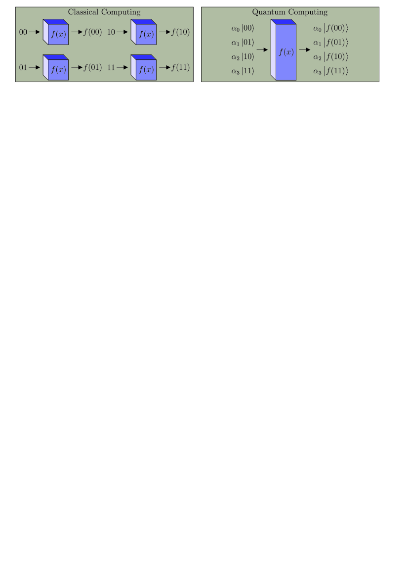
Figure 1: Quantum Parallelism: Given a function $f(x)$, which has a regular global structure such that $f(x):\{0,1\}^{2}\rightarrow\{0,1\}^{2}$, a classical system requires four evaluations to compute $f(x)$ for all possible $x\in\{00,01,10,11\}$. By contrast, since a $2$-qubit quantum register can be in a superposition of all the four states concurrently, i.e. $|\psi\rangle=\alpha_{0}|00\rangle+\alpha_{1}|01\rangle+\alpha_{2}|10\rangle+\alpha_{3}|11\rangle$, quantum computing requires only a single classical evaluation to yield the outcome, which is also in a superposition of all the four possibilities, i.e. $\alpha_{0}|f(00)\rangle+\alpha_{1}|f(01)\rangle+\alpha_{2}|f(10)\rangle+\alpha_{3}|f(11)\rangle$. However, it is not possible to read all the four states because the quantum register collapses to one of the four superimposed states upon measurement. Nevertheless, we may manipulate the resultant superposition of the four possible states before observing the quantum register for the sake of determining a desired property of the function, as in [5, 6, 7, 8].

Therefore, as exemplified by Shor’s factorization algorithm [7] and Grover’s search algorithm [8], quantum-based computation is capable of solving certain complex problems at a substantially lower complexity, as compared to its classical counterpart. From the perspective of telecommunications, this quantum domain parallel processing seems to be a plausible solution for the massive parallel processing required for achieving joint optimization in large-scale communication systems, e.g. quantum assisted multi-user detection [4, 9, 10] and quantum-assisted routing optimization for self-organizing networks [11]. Furthermore, quantum-based communication is capable of supporting secure data dissemination, where any ‘measurement’ or ‘observation’ by an eavesdropper destroys the quantum entanglement, hence intimating the parties concerned [13, 3]. Quantum-based communication has given rise to a new range of security paradigms, which cannot be created using a classical communication system. In this context, quantum key distribution techniques [14, 15], quantum secure direct communication [16, 17] and the recently proposed unconditional quantum location verification [18] are of particular significance.

Unfortunately, a major impediment to the practical realization of quantum computation as well as communication systems is quantum noise, which is conventionally termed as ‘decoherence’ (loss of the coherent quantum state). More explicitly, decoherence is the undesirable interaction of the qubits with the environment [19, 20]. It may be viewed as the undesirable entanglement of qubits with the environment, which perturbs the fragile superposition of states, thus leading to the detrimental effects of noise. The overall decoherence process may be characterized either by bit-flips or phase-flips or in fact possibly both, inflicted on the qubits [19], as depicted in Fig. 2.

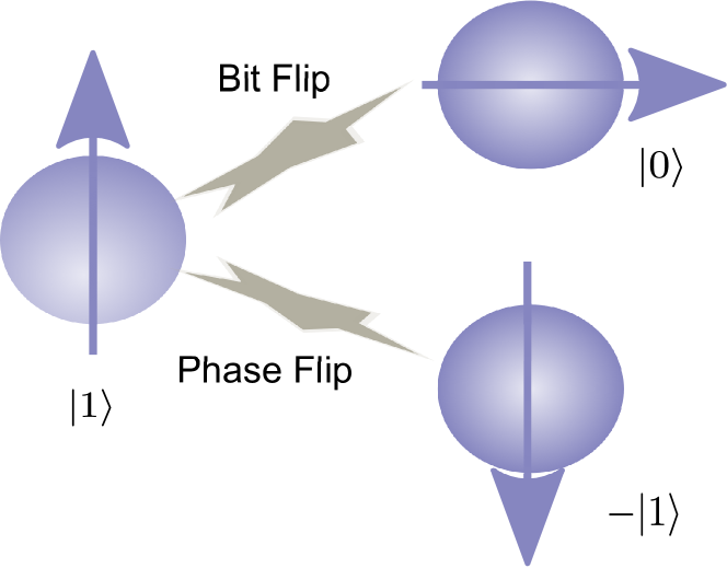
Figure 2: Quantum decoherence characterized by bit and phase flips. The vertical polarization represents the state $|1\rangle$, while the horizontal polarization represents the state $|0\rangle$.

The longer a qubit retains its coherent state (this period is known as the coherence time), the better. This may be achieved with the aid of Quantum Error Correction codes (QECCs), which also rely on the peculiar phenomenon of entanglement - hence John Preskill eloquently pointed out that we are “fighting entanglement with entanglement” [21]. More explicitly, analogously to the classical channel coding techniques, QECCs rectify the impact of quantum noise (bit and phase flips) for the sake of ensuring that the qubits retain their coherent quantum state with a high fidelity, thus in effect beneficially increasing the coherence time of the unperturbed quantum state. This has been experimentally demonstrated in [23, 24, 25].

Similar to the family of classical error correction codes [26, 27], which aim for operating close to Shannon’s capacity limit, QECCs are designed to approach the quantum capacity [28, 29, 30], or more specifically the hashing bound, which is a lower bound of the achievable quantum capacity. A significant amount of work has been carried out over the last few decades to achieve this objective. However, the field of quantum error correction codes is still not as mature as that of their classical counterparts. Recently, inspired by the family of classical near-capacity concatenated codes, which rely on iterative decoding schemes, e.g. [31, 32], substantial efforts have been invested in [33, 34, 35] to construct comparable quantum codes. In the light of this increasing interest in conceiving hashing bound approaching concatenated quantum code design principles, the contributions of this paper are:

1. We survey the evolution towards constructing hashing bound approaching concatenated quantum codes with the aid of EXtrinsic Information Transfer (EXIT) charts. More specifically, to bridge the gap between the classical and quantum channel coding theory, we provide insights into the transformation from the family of classical codes to the class of quantum codes.

2. We propose a generically applicable structure for Quantum Irregular Convolutional Codes (QIRCCs), which can be dynamically adapted to a specific application scenario for the sake of facilitating hashing bound approaching performance. This is achieved with the aid of the EXIT charts of [35].

3. More explicitly, we provide a detailed design example by constructing a $10$-subcode QIRCC and use it as an outer code in concatenation with the non-catastrophic and recursive inner convolutional code of [36, 34]. Our QIRCC-based optimized design outperforms both the design of [34], as well as the exhaustive-search based optimized design of [35].

This paper is organized as follows. We commence by outlining our design objectives in Section II. We then provide a comprehensive historical overview of QECCs in Section III. We detail the underlying stabilizer formalism in Section IV by providing insights into constructing quantum stabilizer codes by cross-pollinating their design with the aid of the well-known classical codes. We then proceed with the design of concatenated quantum codes in Section V, with a special emphasis on their code construction as well as on their decoding procedure. In Section VI, we will detail the EXIT-chart aided code design principles, providing insights into the application of EXIT charts for the design of quantum codes. We will then present our proposed QIRCC design example in Section VII, followed by our simulation results in Section VIII. Finally, our conclusions and design guidelines are offered in Section IX.

II Design Objectives

Meritorious families of quantum error correction codes can be derived from the known classical codes by exploiting the underlying quantum-to-classical isomorphism, while also taking into account the peculiar laws of quantum mechanics. This transition from the classical to the quantum domain must address the following challenges [13]:

• No-Cloning Theorem: Most classical codes are based on the transmission of multiple replicas of the same bit, e.g. in a simple rate-$1/3$ repetition code each information bit is transmitted thrice. This is not possible in the quantum domain according to the no-cloning theorem [37], which states that an arbitrary unknown quantum state cannot be copied/cloned.

• Continuous Nature of Quantum Errors: In contrast to the classical errors, which are discrete with bit-flip being the only type of error, a qubit may experience both a bit error as well as a phase error or in fact both, as depicted in Fig. 2. These impairments have a continuous nature and the erroneous qubit may lie anywhere on the surface of the Bloch sphere.

• Qubits Collapse upon Measurement: ‘Measurement’ of the received bits is a vital step representing a hard-decision operation in the field of classical error correction, but this is not feasible in the quantum domain, since qubits collapse to classical bits upon measurement.

In a nutshell, a classical $(n,k)$ binary code is designed to protect discrete-valued message sequences of length $k$ by encoding them into one of the $2^{k}$ discrete codewords of length $n$. By contrast, since a quantum state of $k$ qubits is specified by $2^{k}$ continuous-valued complex coefficients, quantum error correction aims for encoding a $k$-qubit state into an $n$-qubit state, so that all the $2^{k}$ complex coefficients can be perfectly restored [38]. For example, let $k=2$, then the $2$-qubit information word $|\psi\rangle$ is given by:

$$|\psi\rangle=\alpha_{0}|00\rangle+\alpha_{1}|01\rangle+\alpha_{2}|10\rangle+\alpha_{3}|11\rangle.$$ (1)

Consequently, the error correction algorithm would aim for correctly preserving all the four coefficients, i.e. $\alpha_{0}$, $\alpha_{1}$, $\alpha_{2}$ and $\alpha_{3}$. It is interesting to note here that although the coefficients $\alpha_{0}$, $\alpha_{1}$, $\alpha_{2}$ and $\alpha_{3}$ are continuous in nature, yet the entire continuum of errors can be corrected, if we can correct a discrete set of errors, i.e. bit (Pauli-$\mathbf{X}$), phase (Pauli-$\mathbf{Z}$) as well as both (Pauli-$\mathbf{Y}$) errors inflicted on either or both qubits [13]. This is because measurement results in collapsing the entire continuum of errors to a discrete set. More explicitly, for $|\psi\rangle$ of Eq. (1), the discrete error set is as follows:

$$\{ \mathbf{IX},\mathbf{IZ},\mathbf{IY},\mathbf{XI},\mathbf{XX},\mathbf{XZ},\mathbf{XY},\mathbf{ZI},\mathbf{ZX},\mathbf{ZZ},$$

$$\mathbf{ZY},\mathbf{YI},\mathbf{YX},\mathbf{YZ},\mathbf{YY}\}.$$ (2)

However, the errors $\mathbf{X}$, $\mathbf{Y}$ and $\mathbf{Z}$ may occur with varying frequencies. In this paper, we will focus on the specific design of codes conceived for mitigating the deleterious effects of the quantum depolarizing channel, which has been extensively investigated in the context of QECCs [38, 39, 40]. Briefly, a depolarizing channel, which is characterized by the probability $p$, inflicts an error $\mathcal{P}\in\mathcal{G}_{n}$ on $n$ qubits, where each qubit may independently experience either a bit flip ($\mathbf{X}$), a phase flip ($\mathbf{Z}$) or both ($\mathbf{Y}$) with a probability of $p/3$.

An ideal code $\mathcal{C}$ designed for a depolarizing channel may be characterized in terms of the channel’s depolarizing probability $p$ and its coding rate $R_{Q}$. Here the coding rate $R_{Q}$ is measured in terms of the number of qubits transmitted per channel use, i.e. we have $R_{Q}=k/n$, where $k$ and $n$ are the lengths of the information word and codeword, respectively. Analogously to Shannon’s classical capacity, the relationship between $p$ and $R_{Q}$ for the depolarizing channel is defined by the hashing bound, which sets a lower limit on the achievable quantum capacity. The hashing bound is given by [43, 34]:

$$C_{Q}(p)=1-H_{2}(p)-p\log_{2}(3),$$ (3)

where $H_{2}(p)$ is the binary entropy function. More explicitly, for a given $p$, if a random code $\mathcal{C}$ of a sufficiently long codeword-length is chosen such that its coding rate obeys $R_{Q}\leq C_{Q}(p)$, then $\mathcal{C}$ may yield an infinitesimally low Qubit Error Rate (QBER) for a depolarizing probability of $p$. It must be noted here that intuitively a low QBER corresponds to a high fidelity between the transmitted and the decoded quantum state. More explicitly, for a given value of $p$, $C_{Q}(p)$ gives the hashing limit on the coding rate. Alternatively, for a given coding rate $R_{Q}$, where we have $R_{Q}=C_{Q}(p^{*})$, $p^{*}$ gives the hashing limit on the channel’s depolarizing probability. In duality to the classical domain, this may also be referred to as the noise limit. An ideal quantum code should be capable of ensuring reliable transmission close to the noise limit $p^{*}$. Furthermore, for any arbitrary depolarizing probability $p$, its discrepancy with respect to the noise limit $p^{*}$ may be computed in decibels (dB) as follows [34]:

$$\text{Distance from hashing bound}\triangleq 10\times\log_{10}\left(\frac{p^{*}}{p}\right).$$ (4)

Consequently, our quantum code design objective is to minimize the discrepancy with respect to the hashing bound, thereby yielding a hashing bound approaching code design.

It is pertinent to mention here the Entanglement-Assisted (EA) regime of [44, 45, 46, 47], where the entanglement-assisted code $\mathcal{C}$ is characterized by an additional parameter $c$. Here $c$ is the number of entangled qubits pre-shared between the transmitter and the receiver, thus leading to the terminology of being entanglement-assisted. It is assumed furthermore that these pre-shared entangled qubits are transmitted over a noiseless quantum channel. The resultant EA hashing bound is given by [34, 48]:

$$C_{Q}(p)=1-H_{2}(p)-p\log_{2}(3)+\textup{E},$$ (5)

where the so-called entanglement consumption rate is $\textup{E}=\frac{c}{n}$. Furthermore, the value of $c$ may be varied from $0$ to a maximum of $(n-k)$. For the family of maximally entangled codes associated with $c=(n-k)$, the EA hashing bound of Eq. (5) is reduced to [34, 48]:

$$C_{Q}(p)=1-\frac{H_{2}(p)-p\log_{2}(3)}{2}.$$ (6)

Therefore, the resultant hashing region of the EA communication is bounded by Eq. (3) and Eq. (6), which is also illustrated in Fig. 3.

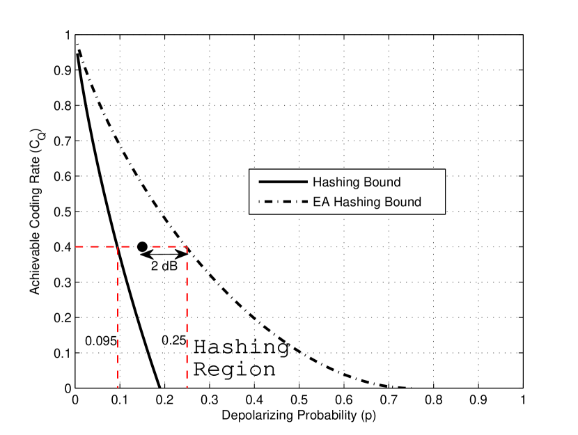
Figure 3: Unassisted and EA hashing bounds characterized by Eq. (3) and Eq. (6), respectively, for the quantum depolarizing channel. The region enclosed by these two bounds, which is labeled the hashing region, defines the capacity for varying number of pre-shared entangled qubits ($c$). At $R_{Q}=0.4$, the unassisted hashing bound gives a noise limit of $p^{*}=0.095$, while the maximally entangled hashing bound increases the limit to $p^{*}=0.25$. The circle represents a maximally entangled code with $R_{Q}=0.4$, which ensures reliable transmission for $p\leq 0.15$, thus operating at a distance of $2$ dB from the noise limit.

To elaborate a little further, let us assume that the desired coding rate is $R_{Q}=0.4$. Then, as gleaned from Fig. 3, the noise limit for the ‘unassisted’ quantum code is around $p^{*}=0.095$, which increases to around $p^{*}=0.25$ with the aid of maximum entanglement, i.e. we have $\textup{E}=1-R_{Q}=0.6$. Furthermore, $0<\textup{E}<0.6$ will result in bearing noise limits in the range of $0.095<p^{*}<0.25$. Let us assume furthermore that we design a maximally entangled code $\mathcal{C}$ for $R_{Q}=0.4$, so that it ensures reliable transmission for $p\leq 0.15$. Based on Eq. (4), the performance of this code (marked with a circle in Fig. 3) is around $[10\times\log 10(\frac{0.25}{0.15})]=2$ dB away from the noise limit. We may approach the noise limit more closely by optimizing a range of conflicting design challenges, which are illustrated in the stylized representation of Fig. 4. For example, we may achieve a lower QBER by increasing the code length. However, this in turn incurs longer delays. Alternatively, we may resort to more complex code designs for reducing the QBER, which may also be reduced by employing codes having lower coding rates or higher entanglement consumption rates, thus requiring more transmitted qubits or entangled qubits. Hence striking an appropriate compromise, which meets these conflicting design challenges, is required.

Figure 4: Stylized illustration of the conflicting design challenges, which are involved in the design of quantum codes.

III Historical Overview of Quantum Error Correction Codes

A major breakthrough in the field of quantum information processing was marked by Shor’s pioneering work on quantum error correction codes, which dispelled the notion that conceiving QECCs was infeasible due to the existence of the no-cloning theorem. Inspired by the classical $3$-bit repetition codes, Shor conceived the first quantum code in his seminal paper [19], which was published in 1995. The proposed code had a coding rate of $1/9$ and was capable of correcting only single qubit errors. This was followed by Calderbank-Shor-Steane (CSS) codes, invented independently by Calderbank and Shor [49] as well as by Steane [50, 51], which facilitated the design of good quantum codes from the known classical binary linear codes. More explicitly, CSS codes may be defined as follows:

An $[n,k_{1}-k_{2}]$ CSS code, which is capable of correcting $t$ bit errors as well as phase errors, can be constructed from classical linear block codes $C_{1}(n,k_{1})$ and $C_{2}(n,k_{2})$, if $C_{2}\subset C_{1}$ and both $C_{1}$ as well as the dual of $C_{2}$, i.e. $C_{2}^{\bot}$, can correct $t$ errors. Here, $C_{1}$ is used for correcting bit errors, while $C_{2}^{\bot}$ is used for phase-error correction.

Therefore, with the aid of CSS construction, the overall problem of finding good quantum codes was reduced to finding good dual-containing or self-orthogonal classical codes. Following these principles, the classical $[7,4,3]$ Hamming code was used to design a $7$-qubit Steane code [51] having a coding rate of $1/7$, which is capable of correcting single isolated errors inflicted on the transmitted codewords. Finally, Laflamme et al.  [52] and Bennett et al.  [43] independently proposed the optimal single error correcting code in 1996, which required only $4$ redundant qubits.

Following these developments, Gottesman formalized the notion of constructing quantum codes from the classical binary and quaternary codes by establishing the theory of Quantum Stabilizer Codes (QSCs) [53] in his Ph.D thesis [54]. In contrast to the CSS construction, the stabilizer formalism defines a more general class of quantum codes, which imposes a more relaxed constraint than the CSS codes. Explicitly, the resultant quantum code structure can either assume a CSS or a non-CSS (also called unrestricted) structure, but it has to meet the symplectic product criterion. More specifically, stabilizer codes constitute a broad class of quantum codes, which subsumes CSS codes as a subclass and has undoubtedly provided a firm foundation for a wide variety of quantum codes developed, including for example quantum Bose-Chaudhuri-Hocquenghem (BCH) codes [55, 56, 57, 58], quantum Reed-Solomon codes [59, 60], Quantum Low Density Parity Check (QLDPC) codes [61, 38, 62, 63], Quantum Convolutional Codes (QCCs) [64, 65, 66, 67], Quantum Turbo Codes (QTCs) [39, 33] as well as quantum polar codes [40, 68, 69]. These major milestones achieved in the history of quantum error correction codes are chronologically arranged in Fig. 5. Let us now look deeper into the development of QCCs, QLDPC codes and QTCs, which have been the prime focus of most recent research both in the classical as well as in the quantum domain.

1995  $-$	Shor’s code [19]
Stabilizer codes [53, 54]  $-$	CSS codes [49, 50, 51], $5$-qubit code [52, 43]
$-$	Quantum BCH codes [55, 56]
$-$
Quantum Reed-Solomon codes [60]  $-$	Quantum Reed-Muller codes [59]
2000  $-$
$-$	Quantum LDPC codes [61]
$-$
$-$	Quantum convolutional codes [64]
$-$
2005  $-$
$-$
$-$
$-$	Quantum turbo codes [39]
$-$
2010  $-$
$-$	Quantum polar codes [40]
$-$

Figure 5: Major milestones achieved in the history of quantum error correction codes.

The inception of QCCs dates back to 1998. Inspired by the higher coding efficiencies of Classical Convolutional Codes (CCCs) as compared to the comparable block codes and the low latency associated with the online encoding and decoding of CCCs [70], Chau conceived the first QCC in [71]. He also generalized the classical Viterbi decoding algorithm for the class of quantum codes in [72], but he overlooked some crucial encoding and decoding aspects. Later, Ollivier et al.  [64, 65] revisited the class of stabilizer-based convolutional codes. Similar to the classical Viterbi decoding philosophy, they also conceived a look-up table based quantum Viterbi algorithm for the maximum likelihood decoding of QCCs, whose complexity increases linearly with the number of encoded qubits. Ollivier et al. also derived the corresponding online encoding and decoding circuits having complexity which increased linearly with the number of encoded qubits. Unfortunately, their proposed rate-$1/5$ single-error correcting QCC did not provide any performance or decoding complexity gain over the rate-$1/5$ single-error correcting block code of [52]. Pursuing this line of research, Almeida et al.  [73] constructed a rate-$1/4$ single-error correcting Shor-type concatenated QCC from a classical CC$(2,1,2)$ and invoked the classical syndrome-based trellis decoding for the quantum domain. Hence, the proposed QCC had a higher coding rate than the QCC of [64, 65]. However, this coding efficiency was achieved at the cost of a relatively high encoding complexity associated with the concatenated trellis structure. It must be pointed out here that the pair of independent trellises used for decoding the bit and phase errors impose a lower complexity than a large joint trellis would. Finally, Forney et al.  [66, 67] designed rate-$(n-2)/n$ QCCs comparable to their classical counterparts, thus providing higher coding efficiencies than the comparable block codes. Forney et al.  [66, 67] achieved this by invoking arbitrary classical self-orthogonal rate-$1/n$ $\mathbb{F}_{4}$-linear and $\mathbb{F}_{2}$-linear convolutional codes for constructing unrestricted and CSS-type QCCs, respectively. Forney et al.  [66, 67] also conceived a simple decoding algorithm for single-error correcting codes. Both the coding efficiency and the decoding complexity of the aforementioned QCC structures are compared in Table TABLE.

Author(s)	Coding Efficiency	Decoding Complexity
Ollivier and Tillich [64, 65]	Low	Moderate
Almeida and Palazzo [73]	Moderate	Moderate
Forney et al.  [66, 67]	High	Low

TABLE: Comparison of the Quantum Convolutional Code (QCC) structures.

Furthermore, in the spirit of finding new constructions for QCCs, Grassl et al.  [74, 75] constructed QCCs using the classical self-orthogonal product codes, while Aly et al. explored various algebraic constructions in [76] and [77], where QCCs were derived from classical BCH codes and Reed-Solomon and Reed-Muller codes, respectively. Recently, Pelchat and Poulin made a major contribution to the decoding of QCCs by proposing degenerate Viterbi decoding [78], which runs the Maximum A Posteriori (MAP) algorithm [27] over the equivalent classes of degenerate errors, thereby improving the attainable performance. The major contributions to the development of QCCs are summarized in Table I.

Year	Author(s)	Contribution
1998	Chau [71]	The first QCCs were developed. Unfortunately, some important encoding/decoding aspects were ignored.
1999	Chau [72]	Classical Viterbi decoding algorithm was generalized to the quantum domain. However, similar to [71], some crucial encoding/decoding aspects were overlooked.
2003	Ollivier and Tillich [64, 65]	Stabilizer-based convolutional codes and their maximum likelihood decoding using the Viterbi algorithm were revisited to overcome the deficiencies of [71, 72]. Failed to provide better performance or decoding complexity than the comparable block codes.
2004	Almeida and Palazzo [73]	Shor-type concatenated QCC was conceived and classical syndrome trellis was invoked for decoding. A high coding efficiency was achieved at the cost of a relatively high encoding complexity.
2005	Forney et al.  [66, 67]	Unrestricted and CSS-type QCCs were derived from arbitrary classical self-orthogonal $\mathbb{F}_{4}$ and $\mathbb{F}_{2}$ CCCs, respectively, yielding a higher coding efficiency as well as a lower decoding complexity than the comparable block codes.
2005	Grassl and Rotteler [74, 75]	Conceived a new construction for QCCs from the classical self-orthogonal product codes.
2007	Aly et al.  [76]	Algebraic QCCs dervied from BCH codes.
2008	Aly et al.  [77]	Algebraic QCCs constructed from Reed-Solomon and Reed-Muller Codes.
2013	Pelchat and Poulin [78]	Degenerate Viterbi decoding was conceived, which runs the MAP algorithm over the equivalent classes of degenerate errors, thereby improving the performance.

TABLE I: Major contributions to the development of Quantum Convolutional Codes (QCCs).

Although convolutional codes provide a somewhat better performance than the comparable block codes, yet they are not powerful enough to yield a capacity approaching performance, when used on their own. Consequently, the desire to operate close to the achievable capacity of Fig. 3 at an affordable decoding complexity further motivated researchers to design beneficial quantum counterparts of the classical LDPC codes [79], which achieve information rates close to the Shannonian capacity limit with the aid of iterative decoding schemes. Furthermore, the sparseness of the LDPC matrix is of particular interest in the quantum domain, because it requires only a small number of interactions per qubit during the error correction procedure, thus facilitating fault-tolerant decoding. Moreover, this sparse nature also makes QLDPC codes highly degenerate. In this context, Postol[61] conceived the first example of a non-dual-containing CSS-based QLDPC code from a finite geometry based classical LDPC in 2001. However, he did not present a generalized formalism for constructing QLDPC codes from the corresponding classical codes. Later, Mackay et al.  [38] proposed various code structures (e.g. bicycle codes and unicycle codes) for constructing QLDPC codes from the family of classical dual-containing LDPC codes. Among the proposed constructions, the bicycle codes were found to exhibit the best performance. It was observed that unlike good classical LDPC codes, which have at most a single overlap between the rows of the Parity Check Matrix (PCM), dual-containing QLDPC codes must have an even number of overlaps. This in turn results in many unavoidable length-4 cycles, which significantly impair the attainable performance of the message passing decoding algorithm. Furthermore, the minimum distance of the proposed codes was upper bounded by the row weight. Additionally, Mackay et al. also proposed the class of Cayley graph-based dual-containing codes in [80], which were further investigated by Couvreur et al. in [81, 82]. Cayley-graph based constructions yield QLDPC codes whose minimum distance has a lower bound, which is a logarithmic function of the code length, thus the minimum distance can be improved by extending the codeword (or block) length, albeit again, only logarithmically. However, this is achieved at the cost of an increased decoding complexity imposed by the row weight, which also increases logarithmically with the code length. Aly et al. contributed to these developments by constructing dual-containing QLDPC codes from finite geometries in [83], while Djordjevic exploited the Balanced Incomplete Block Designs (BIBDs) in [84], albeit neither of these provided any gain over Mackay’s bicycle codes. Furthermore, Lou et al.  [85, 86] invoked the non-dual-containing CSS structure by using both the generator and the PCM of classical Low Density Generator Matrix (LDGM) based codes. Unfortunately, the proposed LDGM based constructions also suffered from length-$4$ cycles, which in turn required a modified Tanner graph and code doping for decoding, thereby imposing a higher decoding complexity. The only exceptions to length-$4$ cycles were constituted by the class of Quasi-Cyclic (QC) QLDPC codes conceived by Hagiwara et al.  [87], whereby the constituent PCMs of non-dual-containing CSS-type QLDPCs were constructed from a pair of QC-LDPC codes found using algebraic combinatorics. The resultant codes had at minimum girth of $6$, but they did not outperform MacKay’s bicycle codes conceived in [38]. Hagiwara’s design of [87] was extended to non-binary QLDPC codes in [88, 89], which operate closer to the hashing limit than MacKay’s bicycle codes. However, having an upper bounded minimum distance remains a deficiency of this construction and the non-binary nature of the code imposes a potentially high decoding complexity. Furthermore, the performance was still not at par with that of the classical LDPC codes. The concept of QC-QLDPC codes was further extended to the class of spatially-coupled QC codes in [90], which outperformed the ‘non-coupled’ design of [87] at the cost of a small coding rate loss. The spatially-coupled QC-QLDPC was capable of achieving a performance similar to that of the non-binary QC-LDPC code only when its block length was considerably higher. While all the aforementioned QLDPC constructions were CSS-based, Camara et al.  [63] were the first authors to conceive non-CSS QLDPC codes. They invoked group theory for deriving QLDPC codes from the classical self-orthogonal quaternary LDPC codes. Later, Tan et al.  [91] proposed several systematic constructions for non-CSS QLDPC codes, four of which were based on classical binary QC-LDPC codes, while one was derived from classical binary LDPC-convolutional codes. Unfortunately, the non-CSS constructions of [63, 91] failed to outperform Mackay’s bicycle codes. Since most of the above-listed QLDPC constructions exhibit an upper bounded minimum distance, topological QLDPCs were derived from Kitaev’s construction in [92, 93, 94]. Amidst these activities, which focused on the construction of QLDPC codes, Poulin et al. were the first scientists to address the decoding issues of QLDPC codes [95]. As mentioned above, most of the QLDPC codes consist of unavoidable length-$4$ cycles. In fact, when QLDPC codes are viewed in the quaternary formalism, i.e. GF($4$), then they must have length-$4$ cycles, which emerge from the symplectic product criterion. These short cycles erode the performance of the classic message passing decoding algorithm. Furthermore, the classic message passing algorithm does not take into account the degenerate nature of quantum codes, rather it suffers from it. This is known as the ‘symmetric degeneracy error’. Hence, Poulin et al. proposed heuristic methods in [95] to alleviate the undesired affects of having short cycles and symmetric degeneracy error, which were further improved in [96]. The major contributions made in the context of QLDPC codes are summarized in Table II, while the most promising QLDPC construction methods are compared in Table III.

		Year	Author(s)	Code Type	Contribution
QLDPC	Code Construction	2001	Postol [61]	Non-dual-containing CSS	The first example of QLDPC code constructed from a finite geometry based classical code. A generalized formalism for constructing QLDPC codes from the corresponding classical codes was not developed.
		2004	Mackay et al.  [38]	Dual-containing CSS	Various code structures, e.g. bicycle codes and unicycle codes, were conceived for constructing QLDPC codes from classical dual-containing LDPC codes. Performance impairment due to the presence of unavoidable length-4 cycles was first pointed out in this work. Minimum distance of the resulting codes was upper bounded by the row weight.
		2005	Lou et al.  [85, 86]	Non-dual-containing CSS	The generator and PCM of classical LDGM codes were exploited for constructing CSS codes. An increased decoding complexity was imposed and the codes had an upper bounded minimum distance.
		2007	Mackay [80]	Dual-containing CSS	Cayley graph-based QLDPC codes were proposed, which had numerous length-$4$ cycles.
			Camara et al.  [63]	Non-CSS	QLDPC codes derived from classical self-orthogonal quaternary LDPC codes were conceived, which failed to outperform MacKay’s bicycle codes.
			Hagiwara et al.  [87]	Non-dual-containing CSS	Quasi-cyclic QLDPC codes were constructed using a pair of quasi-cyclic LDPC codes, which were found using algebraic combinatorics. The resultant codes had at least a girth of $6$, but they failed to outperform MacKay’s constructions given in [38].
		2008	Aly et al.  [83]	Dual-containing CSS	QLDPC codes were constructed from finite geometries, which failed to outperform Mackay’s bicycle codes.
			Djordjevic [84]	Dual-containing CSS	BIBDs were exploited to design QLDPC codes, which failed to outperform Mackay’s bicycle codes.
		2010	Tan et al.  [91]	Non-CSS	Several systematic constructions for non-CSS QLDPC codes were proposed, four of which were based on classical binary quasi-cyclic LDPC codes, while one was derived from classical binary LDPC-convolutional codes. These code designs failed to outperform Mackay’s bicycle codes.
		2011	Couvreur et al.  [81, 82]	Dual-containing CSS	Cayley graph-based QLDPC codes of [80] were further investigated. The lower bound on the minimum distance of the resulting QLDPC was logarithmic in the code length, but this was achieved at the cost of an increased decoding complexity.
			Kasai [88, 89]	Non-dual-containing CSS	Quasi-cyclic QLDPC codes of [87] were extended to non-binary constructions, which outperformed Mackay’s bicycle codes at the cost of an increased decoding complexity. Performance was still not at par with the classical LDPC codes and minimum distance was upper bounded.
			Hagiwara et al.  [90]	Non-dual-containing CSS	Spatially-coupled QC-QLDPC codes were developed, which outperformed the ‘non-coupled’ design of [87] at the cost of a small coding rate loss. Performance was similar to that of [88, 89], but larger block lengths were required.
	Decoding	2008	Poulin et al.  [95]		Heuristic methods were developed to alleviate the performance degradation caused by unavoidable length-$4$ cycles and symmetric degeneracy error.
		2012	Wang et al.  [96]		Feedback mechanism was introduced in the context of the heuristic methods of [95] to further improve the performance.
QTC	Code Construction	2008	Poulin et al.  [39, 33]	Non-CSS	QTCs were conceived based on the interleaved serial concatenation of QCCs. QTCs are free from the decoding issue associated with the length-$4$ cycles and they offer a wider range of code parameters. Degenerate iterative decoding algorithm was also proposed. Unfortunately, QTCs have an upper bounded minimum distance.
		2014	Babar et al.  [35]	Non-CSS	To dispense with the time-consuming Monte Carlo simulations and to facilitate the design of hashing bound approaching QTCs, the application of classical non-binary EXIT charts of [97] was extended to QTCs.
	Decoding	2014	Wilde et al.  [34]		The iterative decoding algorithm of [39, 33] failed to yield performance similar to the classical turbo codes. The decoding algorithm was improved by iteratively exchanging the extrinsic rather than the a posteriori information.

TABLE II: Major contributions to the development of iterative quantum codes.

Code Construction	Short Cycles	Minimum Distance	Delay	Decoding Complexity
Bicycle codes [38]	Yes	Upper Bounded	Standard	Standard
Cayley-graph based codes [80, 81, 82]	Yes	Increases with the code length	Standard	Increases with the code length
LDGM-based codes [85, 86]	Yes	Upper Bounded	Standard	High
Non-binary quasi-cyclic codes [88, 89]	No	Upper Bounded	Standard	High
Spatially-coupled quasi-cyclic codes [90]	No	Upper Bounded	High	High

TABLE III: Comparison of the Quantum Low Density Parity Check (QLDPC) code structures.

Pursuing further the direction of iterative code structures, Poulin et al. conceived QTCs in [39, 33], based on the interleaved serial concatenation of QCCs. Unlike QLDPC codes, QTCs offer a complete freedom in choosing the code parameters, such as the frame length, coding rate, constraint length and interleaver type. Moreover, their decoding is not impaired by the presence of length-$4$ cycles associated with the symplectic criterion. Furthermore, in contrast to QLDPC codes, the iterative decoding invoked for QTCs takes into account the inherent degeneracy associated with quantum codes. However, it was found in [39, 33, 98] that the constituent QCCs cannot be simultaneously both recursive and noncatastrophic. Since the recursive nature of the inner code is essential for ensuring an unbounded minimum distance, whereas the noncatastrophic nature is a necessary condition to be satisfied for achieving decoding convergence to a vanishingly low error rate, the QTCs designed in [39, 33] had a bounded minimum distance. The QBER performance curves of the QTCs conceived in [39, 33] also failed to match the classical turbo codes. This issue was dealt with in [34], where the quantum turbo decoding algorithm of [33] was improved by iteratively exchanging the extrinsic rather than the a posteriori information. Furthermore, in [39, 33, 34], the optimal components of QTCs were found by analyzing their distance spectra, followed by extensive Monte Carlo simulations for the sake of determining the convergence threshold of the resultant QTC. In order to circumvent this time-consuming approach and to facilitate the design of hashing bound approaching QTCs, the application of classical non-binary EXIT charts [97] was extended to QTCs in [35]. An EXIT-chart aided exhaustive-search based optimized QTC was also presented in [35]. The major contributions made in the domain of quantum turbo codes are summarized in Table II.

Some of the well-known classical codes cannot be imported into the quantum domain by invoking the aforementioned stabilizer-based code constructions because the stabilizer codes have to satisfy the stringent symplectic product criterion. This limitation was overcome in [44, 45, 46, 47] with the notion of EA quantum codes, which exploit pre-shared entanglement between the transmitter and receiver. Later, this concept was extended to numerous other code structures, e.g. EA-QLDPC code [99], EA-QCC [100], EA-QTC [36, 34] and EA-polar codes [101]. In [36, 34], it was also found that entanglement-assisted convolutional codes may be simultaneously both recursive as well as non-catastrophic. Therefore, the issue of bounded minimum distance of QTCs was resolved with the notion of entanglement. Furthermore, EA-QLDPC codes are free from length-$4$ cycles in the binary formalism, which in turn results in an impressive performance similar to that of the corresponding classical LDPC codes. Hence, the concept of the entanglement-assisted regime resulted in a major breakthrough in terms of constructing quantum codes, whose behaviour is similar to that of the corresponding classical codes. The major milestones achieved in the history of entanglement-assisted quantum error correction codes are chronologically arranged in Fig. 6.

2000  $-$
$-$
$-$	First EA-QECC constructed [44]
$-$
$-$
2005  $-$
$-$	EA stabilizer formalism [45, 46, 47]
$-$
$-$
$-$	EA quantum LDPC codes [99]
2010  $-$	EA quantum convolutional codes [100]
$-$	EA quantum turbo codes [36, 34]
$-$	EA polar codes [101]

Figure 6: Major milestones achieved in the history of entanglement-assisted quantum error correction codes.

In this contribution, we design a novel QIRCC, which may be used as an outer component in a QTC, or in fact any arbitrary concatenated quantum code structure. Explicitly, the proposed QIRCC may be invoked in conjunction with any arbitrary inner code (both unassisted as well as entanglement-assisted) for the sake of attaining a hashing bound approaching performance with the aid of the EXIT charts of [35]. More specifically, we construct a $10$-subcode QIRCC and use it as the outer code in concatenation with the non-catastrophic and recursive inner convolutional code of [34]. In contrast to the concatenated code of [34], which exhibited a performance within $0.9$ dB of the hashing bound, our QIRCC-based optimized design operates within $0.4$ dB of the noise limit. Furthermore, at a Word Error Rate (WER) of $10^{-3}$, our design outperforms the benchmark designed in [34] by about $0.5$ dB. Our proposed design also yields a lower error rate than the exhaustive-search based optimized design of [35].

IV Stabilizer Formalism

Most of the quantum codes developed to date owe their existence to the theory of stabilizer codes, which allows us to import any arbitrary classical binary as well as quaternary code to the quantum domain. Unfortunately, this is achieved at the cost of imposing restrictions on the code structure, which may adversely impact the performance of the code, e.g. as in QLDPC codes and QTCs, which was discussed in Section III. In this section, we will delve deeper into the stabilizer formalism for the sake of ensuring a smooth transition from the classical to the quantum domain.

IV-A Classical Linear Block Codes

The stabilizer formalism derives its existence from the theory of classical linear block codes. A classical linear block code $C(n,k)$ maps $k$-bit information blocks onto $n$-bit codewords. For small values of $k$ and $n$, this can be readily achieved using a look-up table, which maps the input information blocks onto the encoded message blocks. However, for large values of $k$ and $n$, the process may be simplified using an $k\times n$ generator matrix $G$ as follows:

$$\overline{x}=xG,$$ (7)

where $x$ and $\overline{x}$ are row vectors for information and encoded messages, respectively. Furthermore, $G$ may be decomposed as:

$$G=\left(I_{k}|P\right),$$ (8)

where $I_{k}$ is a ($k\times k$)-element identity matrix and $P$ is a $k\times(n-k)$-element matrix. This in turn implies that the first $k$ bits of the encoded message are information bits, followed by $(n-k)$ parity bits.

At the decoder, syndrome-based decoding is invoked, which determines the position of the channel-induced error using the observed syndromes rather than directly acting on the received codewords. More precisely, each generator matrix is associated with an $(n-k)\times n$-element PCM $H$ which is given by:

$$H=\left(P^{T}|I_{n-k}\right),$$ (9)

and is defined such that $\overline{x}$ is a valid codeword only if,

$$\overline{x}H^{T}=0.$$ (10)

For a received vector $y=\overline{x}+e$, where $e$ is the error incurred during transmission, the error syndrome of length $(n-k)$ is computed as:

$$s=yH^{T}=(\overline{x}+e)H^{T}=\overline{x}H^{T}+eH^{T}=eH^{T},$$ (11)

which is then used for identifying the erroneous parity bit.

Let us consider a simple $3$-bit repetition code, which makes three copies of the intended information bit. More precisely, $k=1$ and $n=3$. It is specified by the following generator matrix:

$$G=\begin{pmatrix}1&1&1\end{pmatrix},$$ (12)

which yields two possible codewords $[111]$ and $[000]$. At the receiver, a decision may be made on the basis of the majority voting. For example, if $y=[011]$ is received, then we may conclude that the transmitted bit was $1$. Alternatively, we may invoke the PCM-based syndrome decoding. According to Eq. (9), the corresponding PCM is given by:

$$H=\begin{pmatrix}1&1&0\\ 1&0&1\end{pmatrix}.$$ (13)

It can be worked out that $yH^{T}=0$ only for the two valid codewords $[111]$ and $[000]$. For all other received codewords, at least one of the two syndrome elements is set to $1$, e.g. when the first bit is corrupted, i.e. $y=[011]$ or $[100]$, $s=[11]$. Table IV enlists all the $1$-bit errors, which may be identified using this syndrome decoding procedure.

Syndrome $(s)$	Index of Error
$[11]$	$1$
$[10]$	$2$
$[01]$	$3$

TABLE IV: Single-bit errors along with the corresponding syndromes for the PCM of Eq. (13).

This process of error correction using generator and parity check matrices is usually preferred due to its compact nature. Generally, $C(n,k)$ code, which encodes a $k$-bit information message into an $n$-bit codeword, would require $2^{k}$ $n$-bit codewords. Thus, it would required a total of $n2^{k}$ bits to completely specify the code space. By contrast, the aforementioned approach only requires $kn$ bits of the generator matrix. Hence, memory resources are saved exponentially and encoding and decoding operations are efficiently implemented. These attractive features of classical block linear codes and the associated PCM-based syndrome decoding [102] have led to the development of quantum stabilizer codes.

IV-B Quantum Stabilizer Codes (QSCs)

Let us recall from Section II that qubits collapse to classical bits upon measurement [13]. This prevents us from directly applying the classical error correction techniques for reliable quantum transmission. Inspired by the PCM-based syndrome decoding of classical codes, Gottesman [53, 54] introduced the notion of stabilizer formalism, which facilitates the design of quantum codes from the classical ones. Analogous to Shor’s pioneering $9$-qubit code [19], stabilizer formalism overcomes the measurement issue by observing the error syndromes without reading the actual quantum information. More specifically, QSCs invoke the PCM-based syndrome decoding approach of classical linear block codes for estimating the errors incurred during transmission.

Fig. 7 shows the general schematic of a quantum communication system relying on a quantum stabilizer code for reliable transmission. An $[n,k]$ QSC encodes the information qubits $|\psi\rangle$ into the coded sequence $|\overline{\psi}\rangle$ with the aid of $(n-k)$ auxiliary (also called ancilla) qubits, which are initialized to the state $|0\rangle$. The noisy sequence $|\hat{\psi}\rangle=\mathcal{P}|\overline{\psi}\rangle$, where $\mathcal{P}$ is the $n$-qubit channel error, is received at the receiver (RX), which engages in a $3$-step process for the sake of recovering the intended transmitted information. More explicitly, RX computes the syndrome of the received sequence $|\hat{\psi}\rangle$ and uses it to estimate the channel error $\tilde{\mathcal{P}}$. The recovery operator $\mathcal{R}$ then uses the estimated error $\tilde{\mathcal{P}}$ to restore the transmitted coded stream. Finally, the decoder, or more specifically the inverse encoder, processes the recovered coded sequence $|\tilde{\overline{\psi}}\rangle$, yielding the estimated transmitted information qubits $|\tilde{\psi}\rangle$.

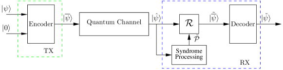
Figure 7: System Model: Quantum communication system relying on a quantum stabilizer code.

An $[n,k]$ quantum stabilizer code, constructed over a code space $\mathcal{C}$, which maps the information word (logical qubits) $|\psi\rangle\in\mathbb{C}^{2^{k}}$ onto the codeword (physical qubits) $|\overline{\psi}\rangle\in\mathbb{C}^{2^{n}}$, where $\mathbb{C}^{d}$ denotes the $d$-dimensional Hilbert space, is defined by a set of $(n-k)$ independent commuting $n$-tuple Pauli operators $g_{i}$, for $1\leq i\leq(n-k)$. The corresponding stabilizer group $\mathcal{H}$ contains both $g_{i}$ and all the products of $g_{i}$ for $1\leq i\leq(n-k)$ and forms an abelian subgroup of $\mathcal{G}_{n}$. A unique feature of these operators is that they do not change the state of valid codewords, while yielding an eigenvalue of $-1$ for corrupted states.

Let us now elaborate on this definition of the stabilizer code by considering a simple $3$-qubit bit-flip repetition code, which is capable of correcting single-qubit bit-flip errors. Since the laws of quantum mechanics do not permit cloning of the information qubit, we cannot encode $|\psi\rangle$ to $(\psi\otimes\psi\otimes\psi)$. Instead, the $3$-qubit bit-flip repetition code entangles two auxiliary qubits with the information qubit such that the basis states $|0\rangle$ and $|1\rangle$ are copied thrice in the superposition of basis states of the resulting $3$-qubit codeword, i.e. $|0\rangle$ and $|1\rangle$ are mapped as follows:

$$|0\rangle \rightarrow|000\rangle,$$

$$|1\rangle \rightarrow|111\rangle.$$ (14)

Consequently, the information word $|\psi\rangle=\alpha|0\rangle+\beta|1\rangle$ is encoded as:

$$\alpha|0\rangle+\beta|1\rangle\rightarrow\alpha|000\rangle+\beta|111\rangle.$$ (15)

The resultant codeword is stabilized by the operators $g_{1}=\mathbf{Z}\mathbf{Z}\mathbf{I}$ and $g_{2}=\mathbf{Z}\mathbf{I}\mathbf{Z}$. Here the term ‘stabilize’ implies that the valid codewords are not affected by the generators $g_{1}$ and $g_{2}$ and yield an eigenvalue of $+1$, as shown below:

$$g_{1}\left[|\overline{\psi}\rangle\right] =\alpha|000\rangle+\beta|111\rangle\equiv|\overline{\psi}\rangle,$$

$$g_{2}\left[|\overline{\psi}\rangle\right] =\alpha|000\rangle+\beta|111\rangle\equiv|\overline{\psi}\rangle.$$ (16)

On the other hand, if a corrupted state $|\hat{\psi}\rangle$ is received, then the stabilizer generators yield an eigenvalue of $-1$, e.g. let $|\hat{\psi}\rangle=|100\rangle+\beta|011\rangle$ where $\mathcal{P}=\mathbf{X}\mathbf{I}\mathbf{I}$, then we have:

$$g_{1}\left[|\hat{\psi}\rangle\right] =-\alpha|100\rangle-\beta|011\rangle\equiv-|\hat{\psi}\rangle,$$

$$g_{2}\left[|\hat{\psi}\rangle\right] =-\alpha|100\rangle-\beta|011\rangle\equiv-|\hat{\psi}\rangle.$$ (17)

More specifically, the eigenvalue is $-1$ if the $n$-tuple Pauli error $\mathcal{P}$ acting on the transmitted codeword $|\overline{\psi}\rangle$ anti-commutes with the stabilizer $g_{i}$ and it is $+1$ if $\mathcal{P}$ commutes with $g_{i}$. Therefore, we have:

$$g_{i}|\hat{\psi}\rangle=\left\{\begin{array}[]{l l}|\overline{\psi}\rangle,&g_{i}\mathcal{P}=\mathcal{P}g_{i}\\ -|\overline{\psi}\rangle,&g_{i}\mathcal{P}=-\mathcal{P}g_{i},\\ \end{array}\right.$$ (18)

where $|\hat{\psi}\rangle=\mathcal{P}|\overline{\psi}\rangle$. Table V enlists the eigenvalues for all possible single-qubit bit-flip errors. The resultant $\pm 1$ eigenvalue gives the corresponding error syndrome $s$, which is $0$ for an eigenvalue of $+1$ and $1$ for an eigenvalue of $-1$, as depicted in Table V.

$|\hat{\psi}\rangle=\mathcal{P}|\overline{\psi}\rangle$	$g_{1}|\hat{\psi}\rangle$	$g_{2}|\hat{\psi}\rangle$	Syndrome ($s$)	Index of Error
$\alpha|100\rangle+\beta|011\rangle$	$-1$	$-1$	$[11]$	$1$
$\alpha|010\rangle+\beta|101\rangle$	$-1$	$+1$	$[10]$	$2$
$\alpha|001\rangle+\beta|110\rangle$	$+1$	$-1$	$[01]$	$3$

TABLE V: Single-qubit bit-flip errors along with the corresponding eigenvalues for $3$-qubit bit-flip repetition code.

A $3$-qubit phase-flip repetition code may be constructed using a similar approach. This is because phase errors in the Hadamard basis $\{|+\rangle,|-\rangle\}$ are similar to the bit errors in the computational basis $\{|0\rangle,|1\rangle\}$. More explicitly, the states $|+\rangle$ and $|-\rangle$ are defined as:

$$|+\rangle \equiv\mathbf{H}|0\rangle=\frac{|0\rangle+|1\rangle}{\sqrt{2}},$$

$$|-\rangle \equiv\mathbf{H}|1\rangle=\frac{|0\rangle-|1\rangle}{\sqrt{2}},$$ (19)

where $\mathbf{H}$ is a single-qubit Hadamard gate, which is given by [13]:

$$\mathbf{H}=\frac{1}{\sqrt{2}}\begin{pmatrix}1&1\\ 1&-1\end{pmatrix}.$$ (20)

Therefore, Pauli-$\mathbf{Z}$ acting on the states $|+\rangle$ and $|-\rangle$ yields:

$$\mathbf{Z}|+\rangle =|-\rangle,$$

$$\mathbf{Z}|-\rangle =|+\rangle,$$ (21)

which is similar to the operation of Pauli-$\mathbf{X}$ on the states $|0\rangle$ and $|1\rangle$, i.e. we have:

$$\mathbf{X}|0\rangle =|1\rangle,$$

$$\mathbf{X}|1\rangle =|0\rangle.$$ (22)

Consequently, analogous to Eq. (14), a $3$-qubit phase-flip repetition code encodes $|0\rangle$ and $|1\rangle$ as follows:

$$|0\rangle \rightarrow|+++\rangle,$$

$$|1\rangle \rightarrow|---\rangle.$$ (23)

Based on Eq. (23), $|\psi\rangle$ is encoded to:

$$\alpha|0\rangle+\beta|1\rangle\rightarrow\alpha|+++\rangle+\beta|---\rangle,$$ (24)

which is stabilized by the generators $g_{1}=\mathbf{X}\mathbf{X}\mathbf{I}$ and $g_{2}=\mathbf{X}\mathbf{I}\mathbf{X}$. Hence, the Hadamard and Pauli-$\mathbf{X}$ operators enable a quantum code to correct phase errors. This overall transition from the classical $3$-bit repetition code of Section IV-A to the quantum repetition code is summarized in Fig. 8.

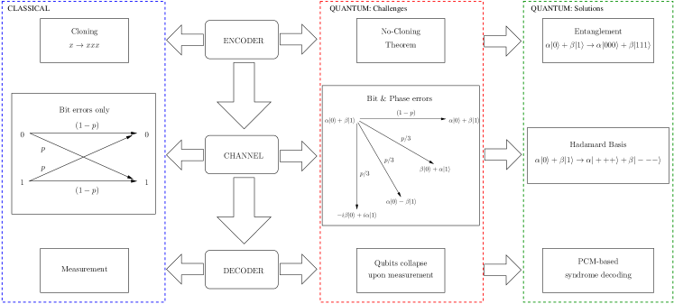
Figure 8: Transition from the classical to quantum codes. Encoder: In classical codes, the information bit may be copied during the encoding process, e.g. in a $3$-bit repetition code. This is not permissible in the quantum domain (no-cloning theorem). Alternatively, in quantum codes, the information qubit is entangled to the auxiliary qubits, e.g. in a $3$-qubit bit-flip repetition code. Channel: Only bit errors occur over a classical channel, e.g. a binary symmetric channel with the channel crossover probability $p$. By contrast, qubits may experience a bit or phase error as well as both, e.g. depolarizing channel with a probability $p$. Since phase errors in the Hadamard basis $\{|+\rangle,|-\rangle\}$ are similar to the bit errors in the computational basis $\{|0\rangle,|1\rangle\}$, phase errors may be corrected in the same way as the bit errors by exploiting the Hadamard basis. Decoder: In classical codes, the received bits are measured during the decoding process, e.g. in a $3$-bit repetition code a decision may be made on the basis of majority voting. Unfortunately, qubits collapse upon measurement. Consequently, quantum codes invoke the PCM-based syndrome decoding.

Furthermore, the stabilizer generators $g_{i}$ constituting the stabilizer group $\mathcal{H}$ must exhibit the following two characteristics:

1. Any two operators in the stabilizer set must commute so that the stabilizer operators can be applied simultaneously, i.e. we have:

   $$g_{1}g_{2}|\overline{\psi}\rangle=g_{2}g_{1}|\overline{\psi}\rangle.$$ (25)

   This is because the stabilizer leaves the codeword unchanged as encapsulated below:

   $$g_{i}|\overline{\psi}\rangle=|\overline{\psi}\rangle.$$ (26)

   Hence, evaluating the left-hand and right-hand sides of Eq. (25) gives:

   $$g_{1}g_{2}|\overline{\psi}\rangle=g_{1}|\overline{\psi}\rangle=|\overline{\psi}\rangle,$$ (27)

   and

   $$g_{2}g_{1}|\overline{\psi}\rangle=g_{2}|\overline{\psi}\rangle=|\overline{\psi}\rangle,$$ (28)

   respectively. This further imposes the constraint that the stabilizers should have an even number of places with different non-Identity (i.e. $\mathbf{X}$, $\mathbf{Y}$, or $\mathbf{Z}$) operations. This is derived from the fact that the $\mathbf{X}$, $\mathbf{Y}$ and $\mathbf{Z}$ operations anti-commute with one another as shown below:

   $$\mathbf{X}\mathbf{Y}=i\mathbf{Z},\;\mathbf{Y}\mathbf{X}=-i\mathbf{Z} \rightarrow\mathbf{X}\mathbf{Y}=-\mathbf{Y}\mathbf{X}$$ (29)

   $$\mathbf{Y}\mathbf{Z}=i\mathbf{X},\;\mathbf{Z}\mathbf{Y}=-i\mathbf{X} \rightarrow\mathbf{Y}\mathbf{Z}=-\mathbf{Z}\mathbf{Y}$$

   $$\mathbf{Z}\mathbf{X}=i\mathbf{Y},\;\mathbf{X}\mathbf{Z}=-i\mathbf{Y} \rightarrow\mathbf{Z}\mathbf{X}=-\mathbf{X}\mathbf{Z}$$

   Thus, for example the operators $\mathbf{ZZI}$ and $\mathbf{XYZ}$ commute, whereas $\mathbf{ZZI}$ and $\mathbf{YZI}$ anti-commute.

2. Generators constituting the stabilizer group $\mathcal{H}$ are closed under multiplication, i.e. multiplication of the constituent generators $g_{i}$ yields another generator, which is also part of the stabilizer group $\mathcal{H}$. For example, the full stabilizer group $\mathcal{H}$ of the $3$-qubit bit-flip repetition code will also include the operator $\mathbf{IZZ}$, which is the product of $g_{1}$ and $g_{2}$.

It must be mentioned here that the Pauli errors which differ only by the stabilizer group have the same impact on all the codewords and therefore can be corrected by the same recovery operations. This gives quantum codes the intrinsic property of degeneracy [78]. More explicitly, the errors $\mathcal{P}$ and $\mathcal{P}^{\prime}=g_{i}\mathcal{P}$ have the same impact on the transmitted codeword and therefore can be corrected by the same recovery operation. Getting back to our example of the $3$-qubit bit-flip repetition code, let $\mathcal{P}=\mathbf{IIX}$ and $\mathcal{P}^{\prime}=g_{1}\mathcal{P}=\mathbf{ZZX}$. Both $\mathcal{P}$ as well as $\mathcal{P}^{\prime}$ corrupt the transmitted codeword of Eq. (15) to $\alpha|001\rangle+\beta|110\rangle$. Consequently, $\mathcal{P}$ and $\mathcal{P}^{\prime}$ need not be differentiated and are therefore classified as degenerate errors.

IV-C Pauli-to-Binary Isomorphism

QSCs may be characterized in terms of an equivalent classical parity check matrix notation satisfying the commutativity constraint of stabilizers [103, 38] given in Eq. (25). This is achieved by mapping the $\mathbf{I}$, $\mathbf{X}$, $\mathbf{Y}$ and $\mathbf{Z}$ Pauli operators onto $(\mathbb{F}_{2})^{2}$ as follows:

$$\mathbf{I} \rightarrow(0,0),$$

$$\mathbf{X} \rightarrow(0,1),$$

$$\mathbf{Y} \rightarrow(1,1),$$

$$\mathbf{Z} \rightarrow(1,0).$$ (30)

More explicitly, the $(n-k)$ stabilizers of an $[n,k]$ stabilizer code constitute the rows of the binary PCM $H$, which can be represented as a concatenation of a pair of $(n-k)\times n$ binary matrices $H_{z}$ and $H_{x}$ based on Eq. (30), as given below:

$$H=\left(H_{z}|H_{x}\right).$$ (31)

Each row of $H$ corresponds to a stabilizer of $\mathcal{H}$, so that the $i$th column of $H_{z}$ and $H_{x}$ corresponds to the $i$th qubit and a binary $1$ at these locations represents a $\mathbf{Z}$ and $\mathbf{X}$ Pauli operator, respectively, in the corresponding stabilizer. For the $3$-qubit bit-flip repetition code, which can only correct bit-flip errors, the PCM $H$ is given by:

$$H=\left(\begin{array}[]{c c c|c c c}1&1&0&0&0&0\\ 1&0&1&0&0&0\end{array}\right).$$ (32)

It must be pointed out here that $H_{z}$ of Eq. (32) is same as the $H$ of the classical repetition code of Eq. (13), yielding the same syndrome patterns in Table IV and Table V.

Let us further elaborate the process by considering the $[9,1]$ Shor’s code, which consists of the Pauli-$\mathbf{Z}$ as well as the Pauli-$\mathbf{X}$ operators. The corresponding stabilizer generators are given in Table VI. They can be mapped onto the binary matrix $H$ as follows:

$$H=\left(\begin{array}[]{c | c}H_{z}^{\prime}&\mathbf{0}\\ \mathbf{0}&H_{x}^{\prime}\end{array}\right),$$ (33)

where we have $H_{z}=\begin{pmatrix}H_{z}^{\prime}\\ \mathbf{0}\end{pmatrix}$, $H_{x}=\begin{pmatrix}\mathbf{0}\\ H_{x}^{\prime}\end{pmatrix}$ and :

$$H_{z}^{\prime}=\begin{pmatrix}1&1&0&0&0&0&0&0&0\\ 0&1&1&0&0&0&0&0&0\\ 0&0&0&1&1&0&0&0&0\\ 0&0&0&0&1&1&0&0&0\\ 0&0&0&0&0&0&1&1&0\\ 0&0&0&0&0&0&0&1&1\\ \end{pmatrix},$$ (34)

$$H_{x}^{\prime}=\begin{pmatrix}1&1&1&1&1&1&0&0&0\\ 0&0&0&1&1&1&1&1&1\end{pmatrix}.$$ (35)

	Stabilizer
$g_{1}$	ZZIIIIIII
$g_{2}$	IZZIIIIII
$g_{3}$	IIIZZIIII
$g_{4}$	IIIIZZIII
$g_{5}$	IIIIIIZZI
$g_{6}$	IIIIIIIZZ
$g_{7}$	XXXXXXIII
$g_{8}$	IIIXXXXXX

TABLE VI: Stabilizers for $9$-qubit Shor’s code.

With the matrix notation of Eq. (31), the commutative property of stabilizers given in Eq. (25) is transformed into the orthogonality of rows with respect to the symplectic product (also called twisted product). If row $m$ is $r_{m}=(z_{m},x_{m})$, where $z_{m}$ and $x_{m}$ are the binary strings for Z and X respectively, then the symplectic product of rows $m$ and $m^{\prime}$ is given by,

$$r_{m}\star r_{m^{\prime}}=(z_{m}\cdot x_{m^{\prime}}+z_{m^{\prime}}\cdot x_{m})\;\text{mod 2}.$$ (36)

This symplectic product is zero if there are even number of places where the operators (X or Z) in row $m$ and $m^{\prime}$ are different; thus meeting the commutativity requirement. In other words, if $H$ is written as $H=(H_{z}|H_{x})$, then the symplectic product is satisfied for all the rows only if,

$$H_{z}H_{x}^{T}+H_{x}H_{z}^{T}=0,$$ (37)

which may be readily verified for the $H$ of Eq. (33). Consequently, any classical binary codes satisfying Eq. (37) may be used to construct QSCs. A special class of these stabilizer codes are CSS codes, which are defined as follows:

An $[n,k_{1}-k_{2}]$ CSS code, which is capable of correcting $t$ bit as well as phase errors, can be constructed from classical linear block codes $C_{1}(n,k_{1})$ and $C_{2}(n,k_{2})$, if $C_{2}\subset C_{1}$ and both $C_{1}$ as well as the dual of $C_{2}$, i.e. $C_{2}^{\bot}$, can correct $t$ errors.

In CSS construction, the PCM $H_{z}^{\prime}$ of $C_{1}$ is used for correcting bit errors, while the PCM $H_{x}^{\prime}$ of $C_{2}^{\bot}$ is used for phase-error correction. Consequently, the PCM of the resultant CSS code takes the form of Eq. (33). $H_{z}^{\prime}$ and $H_{x}^{\prime}$ are now the $(n-k_{1})\times n$ and $k_{2}\times n$ binary matrices, respectively. Furthermore, since $C_{2}\subset C_{1}$, the symplectic condition of Eq. (37) is reduced to $H_{z}^{\prime}H_{x}^{\prime^{T}}=0$. In this scenario, $(n-k_{1}+k_{2})$ stabilizers are applied to $n$ qubits. Therefore, the resultant quantum code encodes $(k_{1}-k_{2})$ information qubits into $n$ qubits. Furthermore, if $H_{z}^{\prime}=H_{x}^{\prime}$, the resultant structure is called dual-containing (or self-orthogonal) code because $H_{z}\prime H_{z}^{\prime^{T}}=0$, which is equivalent to $C_{1}^{\bot}\subset C_{1}$. Hence, stabilizer codes may be sub-divided into various code structures, which are summarized in Fig. 9.

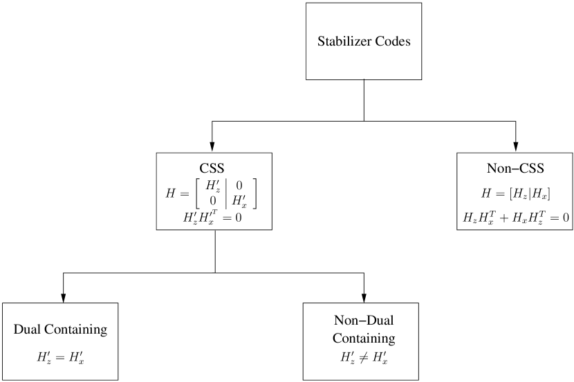
Figure 9: Family of stabilizer codes.

Let us consider the classical $(7,4)$ Hamming code, whose PCM is given by:

$$H=\begin{pmatrix}1&1&0&1&1&0&0\\ 1&0&1&1&0&1&0\\ 0&1&1&1&0&0&1\end{pmatrix}.$$ (38)

Since the $H$ of Eq. (38) yields $HH^{T}=0$, it is used for constructing the dual-containing rate-$1/7$ Steane code [51].

Based on the aforementioned Pauli-to-binary isomorphism, a quantum-based Pauli error operator $\mathcal{P}$ can be represented by the effective classical error pattern $P$, which is a binary vector of length $2n$. More specifically, $P$ is a concatenation of $n$ bits for $\mathbf{Z}$ errors, followed by another $n$ bits for $\mathbf{X}$ errors, as depicted in Fig. 10. An $\mathbf{X}$ error imposed on the $1$st qubit will yield a $0$ and a $1$ at the $1$st and $(n+1)$th index of $P$, respectively. Similarly, a $\mathbf{Z}$ error imposed on the $1$st qubit will give a $1$ and a $0$ at the $1$st and $(n+1)$th index of $P$, respectively, while a $Y$ error on the $1$st qubit will result in a $1$ at both the $1$st as well as $(n+1)$th index of $P$. The resultant syndrome is given by the symplectic product of $\mathbf{H}$ and $P$, which is equivalent to $\mathbf{H}(P_{x}:P_{z})^{T}$. Here colon ($:$) denotes the concatenation operation. In other words, the Pauli-$\mathbf{X}$ operator is used for correcting $\mathbf{Z}$ errors, while the Pauli-$\mathbf{Z}$ operator is used for correcting $\mathbf{X}$ errors [13]. Thus, the quantum-domain syndrome is equivalent to the classical-domain binary syndrome and a basic quantum-domain decoding procedure is similar to syndrome based decoding of the equivalent classical code [38]. However, due to the degenerate nature of quantum codes, quantum decoding aims for finding the most likely error coset, while the classical syndrome decoding [102] finds the most likely error.

Figure 10: Effective classical error $P$ corresponding to the error $\mathcal{P}$ imposed on an $n$-qubit frame.

Hence, an $[n,k]$ quantum stabilizer code associated with $(n-k)$ stabilizers can be effectively modeled using an $(n-k)\times 2n$-element classical PCM satisfying Eq. (37). The coding rate of the equivalent classical code $R_{c}$ can be determined as follows:

$$R_{c} =\frac{2n-(n-k)}{2n}$$

$$=\frac{n+k}{2n}$$

$$=\frac{1}{2}\left(1+\frac{k}{n}\right)$$

$$=\frac{1}{2}\left(1+R_{Q}\right),$$ (39)

where $R_{Q}$ is its quantum coding rate. Using Eq. (39), the coding rate of the classical equivalent of Shor’s rate-$1/9$ quantum code is $5/9$.

IV-D Stabilizer Formalism of Quantum Convolutional Codes

Quantum convolutional codes are derived from the corresponding classical convolutional codes using stabilizer formalism. This is based on the equivalence between the classical convolutional codes and the classical linear block codes with semi-infinite length, which is derived below [26].

Consider a $(2,1,m)$ classical convolutional code with generators,

$$g^{(0)} =(g^{(0)}_{0},g^{(0)}_{1},\dots,g^{(0)}_{m}),$$

$$g^{(1)} =(g^{(1)}_{0},g^{(1)}_{1},\dots,g^{(1)}_{m}).$$ (40)

For an input sequence $[u=(u_{0},u_{1},u_{2},\dots)]$, the output sequences $[v^{(0)}=(v^{(0)}_{0},v^{(0)}_{1},v^{(0)}_{2},\dots)]$ and $[v^{(1)}=(v^{(1)}_{0},v^{(1)}_{1},v^{(1)}_{2},\dots)]$are given as follows:

$$v^{(0)} =u\circledast g^{(0)},$$

$$v^{(1)} =u\circledast g^{(1)},$$ (41)

where $\circledast$ denotes discrete convolution (modulo 2), which implies that for all $l\geq 0$ we have:

$$v_{l}^{(j)}=\sum_{i=0}^{m}u_{l-i}g_{i}^{(j)}=u_{l}g_{0}^{(j)}+u_{l-1}g_{1}^{(j)}+\dots+u_{l-m}g_{m}^{(j)},$$ (42)

where $j=0,1$ and $u_{l-i}\triangleq 0$ for all $l<i$. The two encoded sequences are multiplexed into a single codeword sequence $v$ given by:

$$v=(v_{0}^{(0)},v_{0}^{(1)},v_{1}^{(0)},v_{1}^{(1)},v_{2}^{(0)},v_{2}^{(1)},\dots)$$ (43)

This encoding process can also be represented in matrix notation by interlacing the generators $g^{(0)}$ and $g^{(1)}$ and arranging them in matrix form as follows,

$$G=\begin{pmatrix}g^{(0)(1)}_{0}&g^{(0)(1)}_{1}&\dots&g^{(0)(1)}_{m}\\ &g^{(0)(1)}_{0}&g^{(0)(1)}_{1}&\dots&g^{(0)(1)}_{m}\\ &&g^{(0)(1)}_{0}&g^{(0)(1)}_{1}&\dots&g^{(0)(1)}_{m}\\ &&\ddots&&\dots&\ddots\end{pmatrix},$$ (44)

where $g^{(0)(1)}_{i}\triangleq\left(g^{(0)}_{i}g^{(1)}_{i}\right)$. The encoding operation of Eq. (42) is therefore equivalent to,

$$v=uG.$$ (45)

Since the information sequence $u$ is of arbitrary length, $G$ is semi-infinite. Furthermore, each row of $G$ is identical to the previous row, but is shifted to the right by two places (since $n=2$). In practice, $u$ has a finite length $N$. Therefore, $G$ has $N$ rows and $2(m+N)$ columns for CC$(2,1,m)$. For CC$(n,k,m)$, $G$ can be generalized as follows:

$$G=\begin{pmatrix}G_{0}&G_{1}&\dots&G_{m}\\ &G_{0}&G_{1}&\dots&G_{m}\\ &&G_{0}&G_{1}&\dots&G_{m}\\ &&\ddots&&\dots&\ddots\end{pmatrix},$$ (46)

where $G_{l}$ is a ($k$ x $n$) submatrix with entries,

$$G_{l}=\begin{pmatrix}g_{1,l}^{(0)}&g_{1,l}^{(1)}&\dots&g_{1,l}^{(n-1)}\\ g_{2,l}^{(0)}&g_{2,l}^{(1)}&\dots&g_{2,l}^{(n-1)}\\ \vdots&\vdots&&\vdots\\ g_{k,l}^{(0)}&g_{k,l}^{(1)}&\dots&g_{k,l}^{(n-1)}\end{pmatrix}.$$ (47)

The corresponding PCM $H$ can be represented as a semi-infinite matrix consisting of submatrices $H_{l}$ with dimensions of $(n-k)\times n$. For a convolutional code with constraint length $(m+1)$, $H$ is given by:

$$H=\begin{pmatrix}H_{0}\\ H_{1}&H_{0}\\ H_{2}&H_{1}&H_{0}\\ \vdots&\vdots&\vdots\\ H_{m}&H_{m-1}&H_{m-2}&\dots&H_{0}\\ &H_{m}&H_{m-1}&H_{m-2}&\dots&H_{0}\\ &&\vdots&\vdots&&\vdots\end{pmatrix}.$$ (48)

Therefore, a CCC can be represented as a linear block code with semi-infinite block length. Furthermore, if each row of the submatrices $H_{l}$ is considered as a single block and $h_{j,i}$ is the $i$th row of the $j$th block, then $H$ has a block-band structure after the first $m$ blocks, whereby the successive blocks are time-shifted versions of the first block $(j=0)$ and the adjacent blocks have an overlap of $m$ submatrices. This has been depicted in Fig. 11 and can be mathematically represented as follows:

$$h_{j,i}=[\mathbf{0}^{j\times n},h_{0,i}],\;1\leq i\leq(n-k),\;0\leq j,$$ (49)

where $\mathbf{0}^{j\times n}$ is a row-vector with $(j\times n)$ zeros.

Figure 11: Block-band structure of the semi-infinite classical PCM $H$.

As discussed in Section IV-C, the rows of a classical PCM correspond to the stabilizers of a quantum code. Hence, the quantum stabilizer group $\mathcal{H}$ of an $[n,k,m]$ stabilizer convolutional code is given by [65]:

$$\mathcal{H}=sp\{g_{j,i}=I^{\otimes jn}\otimes g_{0,i}\},\;1\leq i\leq(n-k),\;0\leq j,$$ (50)

where $g_{j,i}$ is the $i$th stabilizer of the $j$th block of the stabilizer group $\mathcal{H}$. Furthermore, $sp$ represents a symplectic group, thus implying that all the stabilizers $g_{j,i}$ must be independent and must commute with each other.

As proposed by Forney in [66, 67], CSS-type QCCs can be derived from the classical self-orthogonal binary convolution codes. Let us consider the rate $1/3$ QCC of [66, 67], which is constructed from a binary rate-$1/3$ CCC with generators:

$$G=\left(\begin{array}[]{c c c | c c c | c c c| c c c|c}1&1&1&1&0&0&1&1&0&0&0&0&\dots\\ 0&0&0&1&1&1&1&0&0&1&1&0&\dots\\ &&&&\ldots&&&&&&&&\end{array}\right).$$ (51)

In $D$-transform notation, these generators are represented as $(1+D+D^{2},1+D^{2},1)$. Each generator is orthogonal to all other generators under the binary inner product, making it a self-orthogonal code. Moreover, the dual $C^{\bot}$ has the capability of correcting $1$ bit. Therefore, based on the CSS construction, the basic stabilizers of the corresponding single-error correcting $[3,1]$ QCC are as follows:

$$g_{0,1} =[\mathbf{XXX},\mathbf{XII},\mathbf{XXI}],$$ (52)

$$g_{0,2} =[\mathbf{ZZZ},\mathbf{ZII},\mathbf{ZZI}].$$ (53)

Other stabilizers of $\mathcal{H}$ are the time-shifted versions of these basic stabilizers as depicted in Eq. (50).

Let us further consider a non-CSS QCC construction given by Forney in [66, 67]. It is derived from the classical self-orthogonal rate-$1/3$ quaternary $(\mathbb{F}_{4})$ convolutional code $C$ having generators $(1+D,1+wD,1+\bar{w}D)$, where $\mathbb{F}_{4}=\{0,1,w,\overline{w}\}$. These generators can also be represented as follows:

$$G=\left(\begin{array}[]{c c c | c c c | c c c|c}1&1&1&1&w&\bar{w}&0&0&0&\dots\\ 0&0&0&1&1&1&1&w&\bar{w}&\dots\\ &&&&\ldots&&&&&\end{array}\right).$$ (54)

Since all these generators are orthogonal under the Hermitian inner product, $C$ is self-orthogonal. Therefore, a $[3,1]$ QCC can be derived from this classical code. The basic generators $g_{0,i}$, for $1\leq i\leq 2$, of the corresponding stabilizer group, $\mathcal{H}$, are generated by multiplying the generators of Eq. (54) with $w$ and $\bar{w}$, and mapping $0$, $w$, $1$, $\bar{w}$ onto $\mathbf{I}$, $\mathbf{X}$, $\mathbf{Y}$ and $\mathbf{Z}$ respectively. The resultant basic stabilizers are as follows:

$$g_{0,1} =\left(\mathbf{XXX},\mathbf{XZY}\right),$$ (55)

$$g_{0,2} =\left(\mathbf{ZZZ},\mathbf{ZYX}\right),$$ (56)

and all other constituent stabilizers of $\mathcal{H}$ can be derived using Eq. (50).

IV-E Entanglement-Assisted Stabilizer Formalism

Let us recall that the classical binary and quaternary codes may be used for constructing stabilizer codes only if they satisfy the symplectic criterion of Eq. (37). Consequently, some of the well-known classical codes cannot be explored in the quantum domain. This limitation can be readily overcome by using the entanglement-assisted stabilizer formalism, which exploits pre-shared entanglement between the transmitter and receiver to embed a set of non-commuting stabilizer generators into a larger set of commuting generators.

Fig. 12 shows the general schematic of a quantum communication system, which incorporates an Entanglement-Assisted Quantum Stabilizer Code (EA-QSC). An $[n,k,c]$ EA-QSC encodes the information qubits $|\psi\rangle$ into the coded sequence $|\overline{\psi}\rangle$ with the aid of $(n-k-c)$ auxiliary qubits, which are initialized to the state $|0\rangle$. Furthermore, the transmitter and receiver share $c$ entangled qubits (ebits) before actual transmission takes place. This may be carried out during the off-peak hours, when the channel is under-utilized, thus efficiently distributing the transmission requirements in time. More specifically, the state $|\phi^{+}\rangle$ of an ebit is given by the following Bell state:

$$|\phi^{+}\rangle=\frac{|00\rangle^{T_{X}R_{X}}+|11\rangle^{T_{X}R_{X}}}{\sqrt{2}},$$ (57)

where $T_{X}$ and $R_{X}$ denotes the transmitter’s and receiver’s half of the ebit, respectively. Similar to the superdense coding protocol of [104], it is assumed that the receiver’s half of the $c$ ebits are transmitted over a noiseless quantum channel, while the transmitter’s half of the $c$ ebits together with the $(n-k-c)$ auxiliary qubits are used to encode the intended $k$ information qubits into $n$ coded qubits. The resultant $n$-qubit codewords $|\overline{\psi}\rangle$ are transmitted over a noisy quantum channel. The receiver then combines his half of the $c$ noiseless ebits with the received $n$-qubit noisy codewords $|\hat{\psi}\rangle$ to compute the syndrome, which is used for estimating the error $\tilde{\mathcal{P}}$ incurred on the $n$-qubit codewords. The rest of the processing at the receiver is the same as that in Fig. 7.

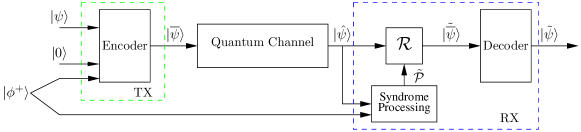
Figure 12: System Model: Quantum communication system relying on an entanglement-assisted quantum stabilizer code

.

The entangled state of Eq. (57) has unique commutativity properties, which aid in transforming a set of non-abelian generators into an abelian set. The state $|\phi^{+}\rangle$ is stabilized by the operators $\mathbf{X}^{T_{X}}\mathbf{X}^{R_{X}}$ and $\mathbf{Z}^{T_{X}}\mathbf{Z}^{R_{X}}$, which commute with each other. Therefore, we have:

$$[\mathbf{X}^{T_{X}}\mathbf{X}^{R_{X}},\mathbf{Z}^{T_{X}}\mathbf{Z}^{R_{X}}]=0.$$ (58)

However, local operators acting on either of the qubits anti-commute, i.e. we have:

$$\{\mathbf{X}^{T_{X}},\mathbf{Z}^{T_{X}}\}=\{\mathbf{X}^{R_{X}},\mathbf{Z}^{R_{X}}\}=0.$$ (59)

Therefore, if we have two single qubit operators $\mathbf{X}^{T_{X}}$ and $\mathbf{Z}^{T_{X}}$, which anti-commute with each other, then we can resolve the anti-commutativity by entangling another qubit and choosing the local operators on this additional qubit such that the resultant two-qubit generators ($\mathbf{X}^{T_{X}}\mathbf{X}^{R_{X}}$ and $\mathbf{Z}^{T_{X}}\mathbf{Z}^{R_{X}}$ for this case) commute. This additional qubit constitutes the receiver half of the ebit. In other words, we entangle an additional qubit for the sake of ensuring that the resultant two-qubit operators have an even number of places with different non-identity operators, which in turn ensures commutativity.

Let us consider a pair of classical binary codes associated with the following PCMs:

$$H_{z}=\begin{pmatrix}0&1&0&0\\ 0&0&0&0\\ 1&1&1&0\\ 0&1&1&1\end{pmatrix},$$ (60)

and

$$H_{x}=\begin{pmatrix}1&0&1&0\\ 1&1&0&1\\ 1&0&0&1\\ 1&1&1&0\end{pmatrix},$$ (61)

which are used to construct a non-CSS quantum code having $H=(H_{z}|H_{x})$. The PCM $H$ does not satisfy the symplectic criterion. The resultant non-abelian set of Pauli generators are as follows:

$$H_{Q}=\left(\begin{array}[]{c c c c}\mathbf{X}&\mathbf{Z}&\mathbf{X}&\mathbf{I}\\ \mathbf{X}&\mathbf{X}&\mathbf{I}&\mathbf{X}\\ \mathbf{Y}&\mathbf{Z}&\mathbf{Z}&\mathbf{X}\\ \mathbf{X}&\mathbf{Y}&\mathbf{Y}&\mathbf{Z}\end{array}\right).$$ (62)

In Eq. (62), the first two generators (i.e. the first and second row) anti-commute, while all other generators commute with each other. This is because the local operators acting on the second qubit in the first two generators anti-commute, while the local operators acting on all other qubits in these two generators commute. In other words, there is a single index (i.e. $2$) with different non-Identity operators. To transform this non-abelian set into an abelian set, we may extend the generators of Eq. (62) with a single additional qubit, whose local operators also anti-commute for the sake of ensuring that the resultant extended generators commute. Therefore, we get:

$$H_{Q}=\left(\begin{array}[]{c c c c | c}\mathbf{X}&\mathbf{Z}&\mathbf{X}&\mathbf{I}&\mathbf{Z}\\ \mathbf{X}&\mathbf{X}&\mathbf{I}&\mathbf{X}&\mathbf{X}\\ \mathbf{Y}&\mathbf{Z}&\mathbf{Z}&\mathbf{X}&\mathbf{I}\\ \mathbf{X}&\mathbf{Y}&\mathbf{Y}&\mathbf{Z}&\mathbf{I}\end{array}\right),$$ (63)

where the operators to the left of the vertical bar $(|)$ act on the transmitted $n$-qubit codewords, while those on the right of the vertical bar act on the receiver’s half of the ebits.

V Concatenated Quantum Codes

In this section, we will lay out the structure of a concatenated quantum code, with a special emphasis on the encoder structure and the decoding algorithm. We commence with the circuit-based representation of quantum stabilizer codes, followed by the system model and then the decoding algorithm.

V-A Circuit-Based Representation of Stabilizer Codes

Circuit-based representation of quantum codes facilitates the design of concatenated code structures. More specifically, for decoding concatenated quantum codes it is more convenient to exploit the circuit-based representation of the constituent codes, rather than the conventional PCM-based syndrome decoding. Therefore, in this section, we will review the circuit-based representation of quantum codes. This discussion is based on [33].

Let us recall from Section IV-A that an $(n,k)$ classical linear block code constructed over the code space $C$ maps the information word $x\in\mathbb{F}^{k}_{2}$ onto the corresponding codeword $\overline{x}\in\mathbb{F}^{n}_{2}$. In the circuit-based representation, this encoding procedure can be encapsulated as follows:

$$C=\{\overline{x}=\left(x:0_{n-k}\right)V\},$$ (64)

where $V$ is an $(n\times n)$-element invertible encoding matrix over $\mathbb{F}_{2}$ and $0_{n-k}$ is an $(n-k)$-bit vector initialized to $0$. Furthermore, given the generator matrix $G$ and the PCM $H$, the encoding matrix $V$ may be specified as:

$$V=\begin{pmatrix}G\\ \left(H^{-1}\right)^{T}\end{pmatrix},$$ (65)

and its inverse is given by:

$$V^{-1}=\begin{pmatrix}G^{-1}&H^{T}\end{pmatrix}.$$ (66)

The encoding matrix $V$ specifies both the code space as well as the encoding operation, while its inverse $V^{-1}$ specifies the error syndrome. More specifically, let $y=\overline{x}+e$ be the received codeword, where $e$ is the $n$-bit error incurred during transmission. Then, passing the received codeword $y$ through the inverse encoder $V^{-1}$ yields:

$$yV^{-1}=\left(\tilde{x}:s\right),$$ (67)

where $\tilde{x}=x+l$ for the logical error $l\in\mathbb{F}^{k}_{2}$ inflicted on the information word $x$ and $s\in\mathbb{F}^{n-k}_{2}$ is the syndrome, which is equivalent to $yH^{T}$. Eq. (67) may be further decomposed to:

$$\left(\overline{x}+e\right)V^{-1} =\left(x+l:s\right),$$

$$\overline{x}V^{-1}+eV^{-1} =\left(x:0_{n-k}\right)+\left(l:s\right),$$ (68)

which is a linear superposition of the inverse of Eq. (64) and $eV^{-1}=\left(l:s\right)$. Hence, the inverse encoder $V^{-1}$ decomposes the channel error $e$ into the logical error $l$ and error syndrome $s$, which is also depicted in Fig. 13.

Figure 13: Circuit representation of the inverse encoder $eV^{-1}=(l:s)$.

Analogously to Eq. (64), the unitary encoding operation $\mathcal{V}$ of an $[n,k]$ QSC, constructed over a code space $\mathcal{C}$, which maps the information word (logical qubits) $|\psi\rangle\in\mathbb{C}^{2^{k}}$ onto the codeword (physical qubits) $|\overline{\psi}\rangle\in\mathbb{C}^{2^{n}}$, may be mathematically encapsulated as follows:

$$\mathcal{C}=\{|\overline{\psi}\rangle=\mathcal{V}(|\psi\rangle\otimes|0_{n-k}\rangle)\},$$ (69)

where $|0_{n-k}\rangle$ are $(n-k)$ auxiliary qubits initialized to the state $|0\rangle$. The unitary encoder $\mathcal{V}$ of Eq. (69) carries out an $n$-qubit Clifford transformation, which maps an $n$-qubit Pauli group $\mathcal{G}_{n}$ onto itself under conjugation [105], i.e. we have:

$$\mathcal{V}\mathcal{G}_{n}\mathcal{V}^{\dagger}=\mathcal{G}_{n}.$$ (70)

In other word, a Clifford operation preserves the elements of the Pauli group under conjugation such that for $\mathcal{P}\in\mathcal{G}_{n}$, $\mathcal{V}\mathcal{P}\mathcal{V}^{\dagger}\in\mathcal{G}_{n}$. Furthermore, any Clifford unitary matrix is completely specified by a combination of Hadamard ($\mathbf{H}$) gates, phase ($\mathbf{S}$) gates and controlled-NOT (C-NOT) gates, which are defined as follows [13]:

$$\mathbf{H}=\frac{1}{\sqrt{2}}\begin{pmatrix}1&1\\ 1&-1\end{pmatrix},\ \mathbf{S}=\begin{pmatrix}1&0\\ 0&i\end{pmatrix},$$

$$\text{C-NOT}=\begin{pmatrix}1&0&0&0\\ 0&1&0&0\\ 0&0&0&1\\ 0&0&1&0\end{pmatrix}.$$ (71)

Hadamard gate preserves the elements of a single-qubit Pauli group $\mathcal{G}_{1}$ as follows:

$$\mathbf{X} \rightarrow\mathbf{H}\mathbf{X}\mathbf{H}^{\dagger}=\mathbf{Z},$$

$$\mathbf{Z} \rightarrow\mathbf{H}\mathbf{Z}\mathbf{H}^{\dagger}=\mathbf{X},$$

$$\mathbf{Y} \rightarrow\mathbf{H}\mathbf{Y}\mathbf{H}^{\dagger}=-\mathbf{Y},$$ (72)

while phase gate preserves them as:

$$\mathbf{X} \rightarrow\mathbf{S}\mathbf{X}\mathbf{S}^{\dagger}=\mathbf{Y},$$

$$\mathbf{Z} \rightarrow\mathbf{S}\mathbf{Z}\mathbf{S}^{\dagger}=\mathbf{Z},$$

$$\mathbf{Y} \rightarrow\mathbf{S}\mathbf{Y}\mathbf{S}^{\dagger}=-\mathbf{X},$$ (73)

Since C-NOT is a $2$-qubit gate, it acts on the elements of $\mathcal{G}_{2}$, transforming the standard basis of $\mathcal{G}_{2}$ as given below:

$$\mathbf{X}\otimes\mathbf{I} \rightarrow\mathbf{X}\otimes\mathbf{X},$$

$$\mathbf{I}\otimes\mathbf{X} \rightarrow\mathbf{I}\otimes\mathbf{X},$$

$$\mathbf{Z}\otimes\mathbf{I} \rightarrow\mathbf{Z}\otimes\mathbf{I},$$

$$\mathbf{I}\otimes\mathbf{Z} \rightarrow\mathbf{Z}\otimes\mathbf{Z}.$$ (74)

Let us further emphasize on the significance of Clifford encoding operation. Since $\mathcal{V}$ belongs to the Clifford group, it preserves the elements of the stabilizer group $\mathcal{H}$ under conjugation. If $g^{\prime}_{i}$ is the $i$th stabilizer of the unencoded state $|\psi\rangle$, then this may be proved as follows:

$$|\psi\rangle\otimes|0_{n-k}\rangle=g^{\prime}_{i}\left(|\psi\rangle\otimes|0_{n-k}\rangle\right).$$ (75)

Encoding $|\psi\rangle$ with $\mathcal{V}$ yields:

$$\mathcal{V}\left(|\psi\rangle\otimes|0_{n-k}\rangle\right)=\mathcal{V}\left(g^{\prime}_{i}\left(|\psi\rangle\otimes|0_{n-k}\rangle\right)\right),$$ (76)

which is equivalent to:

$$\mathcal{V}\left(|\psi\rangle\otimes|0_{n-k}\rangle\right)=\mathcal{V}\left(g^{\prime}_{i}\mathcal{V}^{\dagger}\mathcal{V}\left(|\psi\rangle\otimes|0_{n-k}\rangle\right)\right),$$ (77)

since $\mathcal{V}^{\dagger}\mathcal{V}=\mathbb{I}_{n}$. Substituting Eq. (69) into Eq. (77) gives:

$$|\overline{\psi}\rangle=\left(\mathcal{V}g^{\prime}_{i}\mathcal{V}^{\dagger}\right)|\overline{\psi}\rangle.$$ (78)

Hence, the encoded state $|\overline{\psi}\rangle$ is stabilized by $g_{i}=\mathcal{V}g^{\prime}_{i}\mathcal{V}^{\dagger}$. From this it appears as if any arbitrary $\mathcal{V}$ (not necessarily Clifford) can be used to preserve the stabilizer subspace, which is not true. Since we assume that the stabilizer group $\mathcal{H}$ is a subgroup of the Pauli group, we impose the additional constraint that $\mathcal{V}$ must yield the elements of Pauli group under conjugation as in Eq. (70), which is only true for Clifford operations.

Furthermore, the Clifford encoding operation also preserves the commutativity relation of stabilizers. Let $g^{\prime}_{i}$ and $g^{\prime}_{j}$ be a pair of unencoded stabilizers. Then the above statement can be proved as follows:

$$g_{i}g_{j}=\left(\mathcal{V}g^{\prime}_{i}\mathcal{V}^{\dagger}\right)\left(\mathcal{V}g^{\prime}_{j}\mathcal{V}^{\dagger}\right)=\mathcal{V}g^{\prime}_{i}g^{\prime}_{j}\mathcal{V}^{\dagger}.$$ (79)

Since $g^{\prime}_{i}$ and $g^{\prime}_{j}$ commute, we have:

$$\mathcal{V}g^{\prime}_{i}g^{\prime}_{j}\mathcal{V}^{\dagger}=\mathcal{V}g^{\prime}_{j}g^{\prime}_{i}\mathcal{V}^{\dagger}.$$ (80)

Using $\mathcal{V}^{\dagger}\mathcal{V}=\mathbb{I}_{n}$, gives:

$$\mathcal{V}g^{\prime}_{j}\mathcal{V}^{\dagger}\mathcal{V}g^{\prime}_{i}\mathcal{V}^{\dagger}.=g_{j}g_{i}.$$ (81)

Since the $n$-qubit Pauli group forms a basis for the ($2^{n}\times 2^{n}$)-element matrices of Eq. (71), the Clifford encoder $\mathcal{V}$, which acts on the $2^{n}$-dimensional Hilbert space, can be completely defined by specifying its action under conjugation on the Pauli-$\mathbf{X}$ and $\mathbf{Z}$ operators acting on each of the $n$ qubits, as seen in Eq. (72) to (74). However, $\mathcal{V}$ and $\mathcal{V}^{\prime}$, which differ only through a global phase such that $\mathcal{V}^{\prime}=e^{j\theta}\mathcal{V}$, have the same impact under conjugation. Therefore, global phase has no physical significance in the context of Eq. (70) and the $n$-qubit encoder $\mathcal{V}$ can be completely specified by its action on the binary equivalent of the Pauli operators. More specifically, for an $n$-qubit Clifford transformation, there is an equivalent $2n\times 2n$ binary symplectic matrix $V$, which is given by:

$$[\mathcal{V}\mathcal{P}\mathcal{V}^{\dagger}]=[\mathcal{P}]V=PV,$$ (82)

where $[.]$ denotes the effective Pauli group $G_{n}$ such that $P=[\mathcal{P}]$ differs from $\mathcal{P}$ by a multiplicative constant, i.e. we have $P=\mathcal{P}/\{\pm 1\pm i\}$, and the elements of $G_{n}$ are represented by $2n$-tuple binary vectors based on the mapping given in Eq. (30). As a consequence of this equivalence, any Clifford unitary can be efficiently simulated on a classical system as stated in the Gottesman-Knill theorem [106].

We next define $\mathcal{V}$ by specifying its action on the elements of the Pauli group $\mathcal{G}_{n}$. More precisely, we consider $2n$ $n$-qubit unencoded operators $Z_{i},X_{i},\dots,Z_{n},X_{n}$, where $Z_{i}$ and $X_{i}$ represents the Pauli $\mathbf{Z}$ and $\mathbf{X}$ operator, respectively, acting on the $i$th qubit and the identity $\mathbf{I}$ on all other qubits. The unecoded operators $Z_{k+1},\dots,Z_{n}$ stabilizes the unencoded state of Eq. (69), i.e. $(|\psi\rangle\otimes|0_{n-k}\rangle)$, and are therefore called the unencoded stabilizer generators. On the other hand, $X_{k+1},\dots,X_{n}$ are the unencoded pure errors since $X_{i}$ anti-commutes with the corresponding unencoded stabilizer generator $Z_{i}$, yielding an error syndrome of $1$. Furthermore, the unencoded logical operators acting on the information qubits are $Z_{i},X_{i},\dots,Z_{k},X_{k}$, which commute with the unencoded stabilizers $Z_{k+1},\dots,Z_{n}$. The encoder $\mathcal{V}$ maps the unencoded operators $Z_{i},X_{i},\dots,Z_{n},X_{n}$ onto the encoded operators $\overline{Z}_{i},\overline{X}_{i},\dots,\overline{Z}_{n},\overline{X}_{n}$, which may be represented as follows:

$$\overline{X}_{i}=\left[\mathcal{V}X_{i}\mathcal{V}^{\dagger}\right]=\left[X_{i}\right]V,\;\;\;\;\;\;\overline{Z}_{i}=\left[\mathcal{V}Z_{i}\mathcal{V}^{\dagger}\right]=\left[Z_{i}\right]V.$$ (83)

Since Clifford transformations do not perturb the commutativity relation of the operators, the resultant encoded stabilizers $\overline{Z}_{k+1},\dots,\overline{Z}_{n}$ are equivalent to the stabilizers $g_{i}$ of Eq. (18), while $\overline{X}_{k+1},\dots,\overline{X}_{n}$ are the pure errors $t_{i}$ of the resultant stabilizer code, which trigger a non-trivial syndrome. Moreover, $\overline{Z}_{i},\overline{X}_{i},\dots,\overline{Z}_{k},\overline{X}_{k}$ are the encoded logical operators, which commute with the stabilizers $g_{i}$. Logical operators merely map one codeword onto the other, without affecting the codespace $\mathcal{C}$ of the stabilizer code. It also has to be mentioned here that the stabilizer generators $g_{i}$ together with the encoded logical operations constitute the normalizer of the stabilizer code. The ($2n\times 2n$)-element binary symplectic encoding matrix $V$ is therefore given by:

$$V=\begin{pmatrix}\overline{Z}_{1}\\ \vdots\\ \overline{Z}_{k}\\ \overline{Z}_{k+1}\\ \vdots\\ \overline{Z}_{n}\\ \overline{X}_{1}\\ \vdots\\ \overline{X}_{k}\\ \overline{X}_{k+1}\\ \vdots\\ \overline{X}_{n}\end{pmatrix}=\begin{pmatrix}\overline{Z}_{1}\\ \vdots\\ \overline{Z}_{k}\\ g_{1}\\ \vdots\\ g_{n-k}\\ \overline{X}_{1}\\ \vdots\\ \overline{X}_{k}\\ t_{1}\\ \vdots\\ t_{n-k}\end{pmatrix},$$ (84)

where the Pauli $\mathbf{Z}$ and $\mathbf{X}$ operators are mapped onto the classical bits using the Pauli-to-binary isomorphism of Section IV-C.

Analogously to the classical inverse encoder of Eq. (67), the inverse encoder of a quantum code is the Hermitian conjugate $\mathcal{V}^{\dagger}$. Let $|\hat{\psi}\rangle=\mathcal{P}|\overline{\psi}\rangle$ be the received codeword such that $\mathcal{P}$ is the $n$-qubit channel error. Then, passing the received codeword $|\hat{\psi}\rangle$ through the inverse encoder $\mathcal{V}^{{\dagger}}$ yields:

$$\mathcal{V}^{{\dagger}}\mathcal{P}|\overline{\psi}\rangle =\mathcal{V}^{{\dagger}}\mathcal{P}\mathcal{V}(|\psi\rangle\otimes|0_{(n-k)}\rangle)$$

$$=(\mathcal{L}|\psi\rangle)\otimes(\mathcal{S}|0_{(n-k)}\rangle),$$ (85)

where $\mathcal{V}^{{\dagger}}\mathcal{P}\mathcal{V}\equiv(\mathcal{L}\otimes\mathcal{S})$ and $\mathcal{L}\in\mathcal{G}_{k}$ denotes the error imposed on the information word, while $\mathcal{S}\in\mathcal{G}_{n-k}$ represents the error inflicted on the remaining $(n-k)$ auxiliary qubits. In the equivalent binary representation, Eq. (85) may be modeled as follows:

$$PV^{-1}=\left(L:S\right),$$ (86)

where we have $P=[\mathcal{P}]$, $L=[\mathcal{L}]$ and $S=[\mathcal{S}]$.

Let us now derive the encoding matrix $V$ for the $3$-qubit bit-flip repetition code, which has a binary PCM $H$ given by:

$$H=\left(\begin{array}[]{c c c|c c c}1&1&0&0&0&0\\ 1&0&1&0&0&0\end{array}\right).$$ (87)

The corresponding encoding circuit is depicted in Fig. 14. Its unencoded operators are as follows:

$$\begin{pmatrix}Z_{1}\\ Z_{2}\\ Z_{3}\\ X_{1}\\ X_{2}\\ X_{3}\end{pmatrix}=\begin{pmatrix}\mathbf{ZII}\\ \mathbf{IZI}\\ \mathbf{IIZ}\\ \mathbf{XII}\\ \mathbf{IXI}\\ \mathbf{IIX}\end{pmatrix}\equiv\left(\begin{array}[]{c c c|c c c}1&0&0&0&0&0\\ 0&1&0&0&0&0\\ 0&0&1&0&0&0\\ \hline\cr 0&0&0&1&0&0\\ 0&0&0&0&1&0\\ 0&0&0&0&0&1\end{array}\right).$$ (88)

A C-NOT gate is then applied to the second qubit, which is controlled by the first. As seen in Eq. (74), the C-NOT gate copies Pauli $\mathbf{X}$ operator forward from the control qubit to the target qubit, while $\mathbf{Z}$ is copied in the opposite direction. Therefore, we get:

$$\begin{pmatrix}\mathbf{ZII}\\ \mathbf{IZI}\\ \mathbf{IIZ}\\ \mathbf{XII}\\ \mathbf{IXI}\\ \mathbf{IIX}\end{pmatrix}\underrightarrow{\text{C-NOT}(1,2)}\begin{pmatrix}\mathbf{ZII}\\ \mathbf{ZZI}\\ \mathbf{IIZ}\\ \mathbf{XXI}\\ \mathbf{IXI}\\ \mathbf{IIX}\end{pmatrix}\equiv\left(\begin{array}[]{c c c|c c c}1&0&0&0&0&0\\ 1&1&0&0&0&0\\ 0&0&1&0&0&0\\ \hline\cr 0&0&0&1&1&0\\ 0&0&0&0&1&0\\ 0&0&0&0&0&1\end{array}\right).$$ (89)

Another C-NOT gate is then applied to the third qubit, which is also controlled by the first, yielding:

$$\begin{pmatrix}\mathbf{ZII}\\ \mathbf{ZZI}\\ \mathbf{IIZ}\\ \mathbf{XXI}\\ \mathbf{IXI}\\ \mathbf{IIX}\end{pmatrix}\underrightarrow{\text{C-NOT}(1,3)}\begin{pmatrix}\mathbf{ZII}\\ \mathbf{ZZI}\\ \mathbf{ZIZ}\\ \mathbf{XXX}\\ \mathbf{IXI}\\ \mathbf{IIX}\end{pmatrix} \equiv\left(\begin{array}[]{c c c|c c c}1&0&0&0&0&0\\ 1&1&0&0&0&0\\ 1&0&1&0&0&0\\ \hline\cr 0&0&0&1&1&1\\ 0&0&0&0&1&0\\ 0&0&0&0&0&1\end{array}\right)$$ (96)

$$=V.$$ (97)

As gleaned from Eq. (97), the stabilizer generators of the $3$-qubit bit-flip repetition code are $g_{1}=\mathbf{ZZI}$ and $g_{2}=\mathbf{ZIZ}$. More explicitly, rows $2$ and $3$ of $V$ constitute the PCM $H$ of Eq. (87). The encoded logical operators are $\overline{Z}_{1}=\mathbf{ZII}$ and $\overline{X}_{1}=\mathbf{XXX}$, which commute with the stabilizers $g_{1}$ and $g_{2}$. Finally, the pure errors are $t_{1}=\mathbf{IXI}$ and $t_{2}=\mathbf{IIX}$, which anti-commute with $g_{1}$ and $g_{2}$, respectively, yielding a non-trivial syndrome.

Figure 14: Encoding Circuit for $3$-qubit bit-flip repetition code.

Based on the above discussion, we now proceed to lay out the circuit-based model for a convolutional code, which is given in [33]. As discussed in Section IV-D, convolutional codes are equivalent to linear block codes associated with semi-infinite block lengths. More specifically, as illustrated in Fig. 11, the PCM $H$ of an $(n,k,m)$ convolutional code has a block-band structure, where the adjacent blocks have an overlap of $m$ submatrices. Similarly, the encoder $V$ of a classical convolutional code can be built from repeated applications of a linear invertible seed transformation $U$, which is an $(n+m)\times(n+m)$-element encoding matrix, as shown in Fig. 15. The inverse encoder $V^{-1}$ can be easily obtained by moving backwards in time, i.e. by reading Fig. 15 from right to left. Let us further elaborate by stating that at time instant $j$, the seed transformation matrix $U$ takes as its input the memory bits $m_{j-1}\in\mathbb{F}_{2}^{m}$, the logical bits $l_{j}\in\mathbb{F}_{2}^{k}$ and the syndrome bits $s_{j}\in\mathbb{F}_{2}^{n-k}$ to generate the output bits $e_{j}\in\mathbb{F}_{2}^{n}$ and the memory state $m_{j}$. More explicitly, we have:

$$\left(m_{j}:e_{j}\right)=\left(m_{j-1}:l_{j}:s_{j}\right)U,$$ (98)

and the overall encoder is formulated as [33]:

$$V =U_{[1,\dots,n+m]}U_{[n+1,\dots,2n+m]}\dots U_{[(N-1)n+1,\dots,Nn+m]},$$

$$=\prod_{j=1}^{N}U_{[(j-1)n+1,\dots,jn+m]},$$ (99)

where $N$ denotes the length of the convolutional code and $U_{[(j-1)n+1,\dots,jn+m]}$ acts on $(n+m)$ bits, i.e. $\left(m_{j-2}:l_{j-1}:s_{j-1}\right)$. For an $[n,k,m]$ quantum convolutional code, the seed transformation $U$ is a $2(n+m)\times 2(n+m)$-element symplectic matrix and Eq. (98) may be re-written as:

$$\left(M_{j}:P_{j}\right)=\left(M_{j-1}:L_{j}:S_{j}\right)U,$$ (100)

where $M$ represents the memory state with an $m$-qubit Pauli operator.

Figure 15: Circuit representation of the encoder $V$ of a convolutional code [33].

The aforementioned methodology conceived for constructing the circuit-based model of unassisted quantum codes may be readily extended to the class of entanglement-assisted codes [34]. The unitary encoding operation $\mathcal{V}$ of an $[n,k,c]$ EA-QSC, which acts only on the $n$ transmitter qubits, may be mathematically modeled as follows:

$$\mathcal{C}=\{|\overline{\psi}\rangle=\mathcal{V}(|\psi\rangle^{T_{X}}\otimes|0_{a}\rangle^{T_{X}}\otimes|\phi^{+}_{c}\rangle^{T_{X}R_{X}})\},$$ (101)

where the superscripts $T_{X}$ and $R_{X}$ denote the transmitter’s and receiver’s qubits, respectively. Furthermore, $|0_{a}\rangle^{T_{X}}$ are $a$ auxiliary qubits initialized to the state $|0\rangle$, where $a=(n-k-c)$, and $|\phi^{+}_{c}\rangle^{T_{X}R_{X}}$ are the $c$ entangled qubits. Analogously to Eq. (85), the inverse encoder of an entanglement-assisted quantum code $\mathcal{V}^{{}^{\dagger}}$ gives:

$$\mathcal{V}^{{\dagger}}\mathcal{P}|\overline{\psi}\rangle =\mathcal{V}^{{\dagger}}\mathcal{P}\mathcal{V}(|\psi\rangle^{T_{X}}\otimes|0_{a}\rangle^{T_{X}}\otimes|\phi^{+}_{c}\rangle^{T_{X}R_{X}})$$

$$=(\mathcal{L}^{T_{X}}|\psi\rangle^{T_{X}})\otimes(\mathcal{S}^{T_{X}}|0_{a}\rangle^{T_{X}}\otimes(\mathcal{E}^{T_{X}}|\phi^{+}_{c}\rangle^{T_{X}R_{X}}),$$ (102)

where $\mathcal{L}^{T_{X}}\in\mathcal{G}_{k}$ denotes the error imposed on the information word, while $\mathcal{S}^{T_{X}}\in\mathcal{G}_{a}$ represents the error inflicted on the transmitter’s $a$ auxiliary qubits and $\mathcal{E}^{T_{X}}\in\mathcal{G}_{c}$ is the error corrupting the transmitter’s half of $c$ ebits. The equivalent binary representation of Eq. (102) is given by:

$$PV^{-1}=\left(L:S:E\right),$$ (103)

where we have $P=[\mathcal{P}^{T_{X}}]$, $L=[\mathcal{L}^{T_{X}}]$, $S=[\mathcal{S}^{T_{X}}]$ and $E=[\mathcal{E}^{T_{X}}]$. Similarly, Eq. (100) can be re-modeled as follows:

$$\left(M_{j}:P_{j}\right)=\left(M_{j-1}:L_{j}:S_{j}:E_{j}\right)U.$$ (104)

V-B System Model: Concatenated Quantum Codes

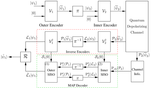
Figure 16: System Model: Quantum communication system relying on concatenated quantum stabilizer codes. $\textup{P}^{a}_{i}(.)$, $\textup{P}^{e}_{i}(.)$ and $\textup{P}^{o}_{i}(.)$ denote the a-priori, extrinsic and a-posteriori probabilities related to the $i$th decoder.

Fig. 16 shows the general schematic of a quantum communication system relying on a pair of concatenated quantum stabilizer codes. In this contribution, both the inner as well as the outer codes are assumed to be convolutional codes. Furthermore, analogously to the classical concatenated codes, the inner code must be recursive, while both the inner as well the outer code must be non-catastrophic. Having a recursive nature of the inner code is essential for the sake of ensuring that the resultant families of codes have an unbounded minimum distance. On the other hand, the non-catastrophic nature of both the inner and the outer codes guarantees that a decoding convergence to an infinitesimally low error rate is achieved. It was found in [39, 98] that QCCs cannot be simultaneously recursive and non-catastrophic. In order to overcome this problem, Wilde et al. [36, 34] proposed to employ entanglement-assisted inner codes, which are recursive as well as non-catastrophic. Therefore, the inner code should be an entanglement-assisted recursive and non-catastrophic code, while the outer code can be either an unassisted or an entanglement-assisted non-catastrophic code.

At the transmitter, the intended quantum information $|\psi_{1}\rangle$ is encoded by an $[n_{1},k_{1}]$ outer encoder $\mathcal{V}_{1}$ using $(n_{1}-k_{1})$ auxiliary qubits, which are initialized to the state $|0\rangle$, as depicted in Eq. (69). The encoded qubits $|\overline{\psi}_{1}\rangle$ are passed through a quantum interleaver ($\pi$). The resultant permuted qubits $|\psi_{2}\rangle$ are fed to an $[n_{2},k_{2}]$ inner encoder $\mathcal{V}_{2}$, which encodes them into the codewords $|\overline{\psi}_{2}\rangle$ using $(n_{2}-k_{2})$ auxiliary qubits initialized to the state $|0\rangle$. The $n$-qubit codewords $|\overline{\psi}_{2}\rangle$, where we have $n=n_{1}n_{2}$, are then serially transmitted over a quantum depolarizing channel, which imposes an $n$-tuple error $\mathcal{P}_{2}\in\mathcal{G}_{n}$ on the transmitted codewords.

At the receiver, the received codeword $|\hat{\psi}_{2}\rangle=\mathcal{P}_{2}|\overline{\psi}_{2}\rangle$ is passed through the inverse encoder $\mathcal{V}_{2}^{{\dagger}}$, which yields the corrupted information word of the inner encoder $\mathcal{L}_{2}|\psi_{2}\rangle$ and the associated $(n_{2}-k_{2})$-qubit syndrome $\mathcal{S}_{2}|0_{(n_{2}-k_{2})}\rangle$ as depicted previously in Eq. (85), where $\mathcal{L}_{2}$ denotes the error imposed on the logical qubits of the inner encoder, while $\mathcal{S}_{2}$ represents the error inflicted on the remaining $(n_{2}-k_{2})$ qubits. The corrupted logical qubits of the inner encoder are de-interleaved, resulting in $\mathcal{P}_{1}|\overline{\psi}_{1}\rangle$, which is then passed through the inverse outer encoder $\mathcal{V}_{1}^{\dagger}$. This gives the corrupted information word of the outer encoder $\mathcal{L}_{1}|\psi_{1}\rangle$ and the associated $(n_{1}-k_{1})$-qubit syndrome $\mathcal{S}_{1}|0_{(n_{1}-k_{1})}\rangle$.

The next step is to estimate the error $\mathcal{L}_{1}$ for the sake of ensuring that the original logical qubit $|\psi_{1}\rangle$ can be restored by applying the recovery operation $\mathcal{R}$. For estimating $\mathcal{L}_{1}$, both the syndromes $\mathcal{S}_{2}|0_{(n_{2}-k_{2})}\rangle$ and $\mathcal{S}_{1}|0_{(n_{1}-k_{1})}\rangle$ are fed to the inner and outer Soft-In Soft-Out (SISO) decoders [27], respectively, which engage in iterative decoding [33, 34] in order to yield the estimated error $\tilde{\mathcal{L}}_{1}$. The corresponding block is marked as ‘MAP Decoder’ in Fig. 16. Here, $\textup{P}^{a}_{i}(.)$, $\textup{P}^{e}_{i}(.)$ and $\textup{P}^{o}_{i}(.)$ denote the a-priori, extrinsic and a-posteriori probabilities [27] related to the $i$th decoder. Based on this notation, the turbo decoding process can be summarized as follows:

• The inner SISO decoder of Fig. 16 uses the channel information $\textup{P}_{\text{ch}}(\mathcal{P}_{2})$, the a-priori information gleaned from the outer decoder $\textup{P}_{2}^{a}(\mathcal{L}_{2})$ (initialized to be equiprobable for the first iteration) and the syndrome $\mathcal{S}_{2}$ to compute the extrinsic information $\textup{P}_{2}^{e}(\mathcal{L}_{2})$. For a coded sequence of length $N$, we have $\mathcal{P}_{2}=[\mathcal{P}_{2,1},\mathcal{P}_{2,2},\dots,\mathcal{P}_{2,t},\dots,\mathcal{P}_{2,N}]$, where $\mathcal{P}_{2,t}=[\mathcal{P}_{2,t}^{1},\mathcal{P}_{2,t}^{2},\dots,\mathcal{P}_{2,t}^{n}]$. The channel information $\mathbf{P}_{\text{ch}}\left(P_{2,t}\right)$ is computed assuming that each qubit is independently transmitted over a quantum depolarizing channel having a depolarizing probability of $p$, whose channel transition probabilities are given by [33]:

  $$\mathbf{P}_{\text{ch}}\left(P_{2,t}^{i}\right)=\left\{\begin{array}[]{l l}1-p,&\text{if }\mathcal{P}_{2,t}^{i}=\mathbf{I}\\ p/3,&\text{if }\mathcal{P}_{2,t}^{i}\in\{\mathbf{X},\mathbf{Z},\mathbf{Y}\}.\\ \end{array}\right.$$ (105)

• $\textup{P}_{2}^{e}(\mathcal{L}_{2})$ is passed through the quantum de-interleaver $(\pi^{-1})$ of Fig. 16 to generate the a-priori information for the outer decoder $\textup{P}_{1}^{a}(\mathcal{P}_{1})$.

• Based on both the a-priori information $\textup{P}_{1}^{a}(\mathcal{P}_{1})$ and on the syndrome $\mathcal{S}_{1}$, the outer SISO decoder of Fig. 16 computes both the a-posteriori information $\textup{P}_{1}^{o}(\mathcal{L}_{1})$ and the extrinsic information $\textup{P}_{1}^{e}(\mathcal{P}_{1})$.

• $\textup{P}_{1}^{e}(\mathcal{P}_{1})$ is then interleaved to obtain $\textup{P}_{2}^{a}(\mathcal{L}_{2})$, which is fed back to the inner SISO decoder of Fig. 16. This iterative procedure continues, until either convergence is achieved or the maximum affordable number of iterations is reached.

• Finally, a qubit-based MAP decision is made for determining the most likely error coset $\mathcal{L}_{1}$. It must be mentioned here that both the inner and outer SISO decoders employ the degenerate decoding approach of [33], which aims for finding the ‘most likely error coset’ rather than the ‘most likely error’ acting on the logical qubits $\mathcal{L}_{i}$, as we will discuss in the next section.

V-C Degenerate Iterative Decoding

As discussed in Section IV-B, quantum codes exhibit the intrinsic property of degeneracy, which is also obvious from Eq. (85). More explicitly, we have:

$$\mathcal{S}|0_{n-k}\rangle=\mathcal{S}_{1}|0\rangle\otimes\dots\otimes\mathcal{S}_{n-k}|0\rangle.$$ (106)

Since, we have $\mathcal{S}_{i}\in\{\mathbf{I},\mathbf{X},\mathbf{Y},\mathbf{Z}\}$, we can re-write Eq. (106) as follows [33]:

$$\mathcal{S}|0_{n-k}\rangle\equiv\epsilon|s_{1}\rangle\otimes\dots\otimes|s_{n-k}\rangle,$$ (107)

where $\epsilon\in\{\pm 1,\pm i\}$, and:

$$s_{i} =0\;\;\;\;\text{if }\mathcal{S}_{i}=\mathbf{I}\;\text{or}\;\mathcal{S}_{i}=\mathbf{Z},$$

$$s_{i} =1\;\;\;\;\text{otherwise}.$$ (108)

For example, if $\mathcal{S}_{1}=\mathbf{Y}$ and $\mathcal{S}_{i}=\mathbf{I}$ for $i\neq 1$, since $\mathbf{Y}=i\mathbf{X}\mathbf{Z}$, we get $\mathcal{S}|0_{n-k}\rangle=i|1\rangle\otimes|0\rangle\otimes\dots\otimes|0\rangle$.

Observing the $(n-k)$ syndrome qubits of Eq. (107) collapses them to the classical syndrome $s=\{s_{1},\dots,s_{n-k}\}$, which is equivalent to the symplectic product of $P$ and $H$, i.e. $s=\left(P\star H_{i}\right)_{1\leq i\leq n-k}$. More precisely, the syndrome sequence $|0_{n-k}\rangle$ is invariant to the $\mathbf{Z}$-component of $\mathcal{S}$ since $\mathbf{Z}|0\rangle=|0\rangle$. Let $S$ be the effective $2(n-k)$-bit error on the syndrome, which may be decomposed as $S=S^{x}+S^{z}$, where $S^{x}$ and $S^{z}$ are the $\mathbf{X}$ and $\mathbf{Z}$ components of $S$, respectively. Then $s$ only reveals $S^{x}$. Hence, two distinct error sequences $P=(L:S^{x}+S^{z})V$ and $P^{\prime}=(L:S^{x}+S^{\prime z})V$, which only differ in the $\mathbf{Z}$-component of $\mathcal{S}$, yield the same syndrome $s$. Furthermore, it must be noted that both $P$ and $P^{\prime}$ have the same logical error $L$. Therefore, $P$ and $P^{\prime}$ differ only by the stabilizer group and are known as degenerate errors, which do not have to be distinguished, since they can be corrected by the same recovery operation $L^{-1}$.

Recall that a classical syndrome-based MAP decoder aims for finding the most likely error for a given syndrome, which may be modeled as:

$$L(S)=\text{argmax}_{L}\textup{P}(L|S),$$ (109)

where $\textup{P}(L|S)$ denotes the probability of experiencing the logical error $L$ imposed on the transmitted qubits, given that the syndrome of the received qubits is $S$. By contrast, quantum codes employ degenerate decoding, which aims for finding the most likely error coset $C(L,S^{x})$ associated with the observed syndrome $S^{x}$. The coset $C(L,S^{x})$ is defined as [33]:

$$C(L,S^{x})=\{P=(L:S^{x}+S^{z})V\}\;\;\;\forall S^{z}\in\{\mathbf{I},\mathbf{Z}\}^{n-k}.$$ (110)

Therefore, a degenerate MAP decoder yields:

$$L(S^{x})=\text{argmax}_{L}\textup{P}(L|S^{x}),$$ (111)

where we have:

$$\textup{P}(L|S^{x})\equiv\sum_{S^{z}\in\{\mathbf{I},\mathbf{Z}\}^{n-k}}\textup{P}(L|(S^{x}+S^{z})).$$ (112)

Figure 17: General schematic of a SISO decoder. $\textup{P}^{a}(.)$, $\textup{P}^{e}(.)$ and $\textup{P}^{o}(.)$ denote the a-priori, extrinsic and a-posteriori probabilities.

The MAP decoder of Fig. 16 consists of two serially concatenated SISO decoders, which employ the aforementioned degenerate decoding approach. Fig. 17 shows the general schematic of a SISO decoder, where the Pauli operators $\mathcal{P}$, $\mathcal{L}$ and $\mathcal{S}$ are replaced by the effective operators $P$, $L$ and $S^{x}$, respectively. The SISO decoder of Fig. 17 yields the a-posteriori information pertaining to $L$ and $P$ based on the classic forward-backward recursive coefficients $\alpha$ and $\beta$, as follows [33]:

• For a coded sequence of duration $N$, let $P=[P_{1},P_{2},\dots,P_{t},\dots,P_{N}]$ and $L=[L_{1},L_{2},\dots,L_{t},\dots,L_{N}]$, where $P_{t}\in G_{n}$ and $L_{t}\in G_{k}$. More explicitly, $P_{t}=[P_{t}^{1},P_{t}^{2},\dots,P_{t}^{n}]$ and $L_{t}=[L_{t}^{1},L_{t}^{2},\dots,L_{t}^{k}]$.

• Let us decompose the seed transformation as $U=(U_{M}:U_{P})$, where $U_{M}$ is the binary matrix formed by the first $2m$ columns of $U$, while $U_{P}$ is the binary matrix formed by the last $2n$ columns of $U$. Therefore, we have:

  $$M_{t}=\left(M_{t-1}:L_{t}:S_{t}\right)U_{M},$$ (113)

  $$P_{t}=\left(M_{t-1}:L_{t}:S_{t}\right)U_{P}.$$ (114)

• Let $\alpha_{t}\left(M_{t}\right)$ be the forward recursive coefficient, which is defined as follows:

  $$\alpha_{t}\left(M_{t}\right) \triangleq\textup{P}\left(M_{t}|S^{x}_{\leq t}\right),$$

  $$\propto\sum_{\begin{subarray}{c}\mu,\lambda,\sigma\end{subarray}}\textup{P}^{a}\left(L_{t}=\lambda\right)\textup{P}^{a}\left(P_{t}\right)\alpha_{t-1}\left(\mu\right),$$ (115)

  where $S^{x}_{\leq t}\triangleq\left(S^{x}_{j}\right)_{0\leq j\leq t}$, $\mu\in G_{m}$, $\lambda\in G_{k}$ and $\sigma\in G_{n-k}$, while $\sigma=\sigma_{x}+\sigma_{z}$, having $\sigma_{x}=S^{x}_{t}$. Furthermore, we have $P_{t}=(\mu:\lambda:\sigma)U_{P}$ and $M_{t}=\left(\mu:\lambda:\sigma\right)U_{M}$.

• Let $\beta_{t}\left(M_{t}\right)$ be the backward recursive coefficient, which is defined as:

  $$\beta_{t}\left(M_{t}\right) \triangleq\textup{P}\left(M_{t}|S^{x}_{>t}\right),$$

  $$\propto\sum_{\lambda,\sigma}\textup{P}^{a}\left(L_{t}=\lambda\right)\textup{P}^{a}\left(P_{t+1}\right)\beta_{t+1}\left(M_{t+1}\right),$$ (116)

  where $S^{x}_{>t}\triangleq\left(S^{x}_{j}\right)_{t<j\leq N}$, $P_{t+1}=(M_{t}:\lambda:\sigma)U_{P}$ and $M_{t+1}=\left(M_{t}:\lambda:\sigma\right)U_{M}$.

• Finally, we have the a-posteriori probabilities $\textup{P}^{o}(L_{t})$ and $\textup{P}^{o}(P_{t})$, which are given by:

  $$\textup{P}^{o}(L_{t}) \triangleq\textup{P}(L_{t}|S^{x}),$$

  $$\propto\sum_{\mu,\sigma}\textup{P}^{a}(L_{t})\textup{P}^{a}(P_{t})\alpha_{t-1}\left(\mu\right)\beta_{t}\left(M_{t}\right),$$ (117)

  $$\textup{P}^{o}(P_{t}) \triangleq\textup{P}(P_{t}|S^{x}),$$

  $$\propto\sum_{\begin{subarray}{c}\mu,\lambda,\sigma\end{subarray}}\textup{P}^{a}(P_{t})\textup{P}^{a}(L_{t}=\lambda)\alpha_{t-1}\left(\mu\right)\beta_{t}\left(M_{t}\right),$$ (118)

  where $S^{x}\triangleq\left(S^{x}_{t}\right)_{0\leq t\leq N}$, $P_{t}=(\mu:L_{t}:\sigma)U_{P}$ and $M_{t}=\left(\mu:L_{t}:\sigma\right)U_{M}$.

• The marginalized probabilities $\textup{P}^{o}(L^{j}_{t})$, for $j\in\{0,k-1\}$, and $\textup{P}^{o}(P^{j}_{t})$, for $j\in\{0,n-1\}$, are then computed from $\textup{P}^{o}(L^{j}_{t})$ and $\textup{P}^{o}(P^{j}_{t})$, respectively. The a-priori information is then removed in order to yield the extrinsic probabilities [34], i.e we have:

  $$\ln[\textup{P}^{e}(L^{j}_{t})] =\ln[\textup{P}^{o}(L^{j}_{t})]-\ln[\textup{P}^{a}(L^{j}_{t})],$$ (119)

  $$\ln[\textup{P}^{e}(P^{j}_{t})] =\ln[\textup{P}^{o}(P^{j}_{t})]-\ln[\textup{P}^{a}(P^{j}_{t})].$$ (120)

It has to be mentioned here that the property of degeneracy is only an attribute of auxiliary qubits and the ebits of an entanglement-assisted code do not contribute to it. This is because both $\mathbf{X}$ as well as $\mathbf{Z}$ errors acting on the transmitter’s half of ebits give distinct results when measured in the Bell basis, i.e. $\mathcal{E}^{T_{X}}|\phi_{c}^{+}\rangle^{T_{X}R_{X}}$ gives four distinct Bell states for $\mathcal{E}_{j}^{T_{X}}\in\{\mathbf{I},\mathbf{X},\mathbf{Z},\mathbf{Y}\}$. Consequently, the degeneracy is a function of $a$ and reduces to zero for $a=0$.

VI EXIT-Chart Aided Code Design

EXIT charts [32, 27, 107] are capable of visualizing the convergence behaviour of iterative decoding schemes by exploiting the input/output relations of the constituent decoders in terms of their average Mutual Information (MI) characteristics. The EXIT chart analysis not only allows us to dispense with the time-consuming Monte-Carlo simulations, but also facilitates the design of capacity approaching codes without resorting to the tedious analysis of their distance spectra. Therefore, they have been extensively employed for designing near-capacity classical codes [108, 109, 110, 111]. Let us recall that the EXIT chart of a serially concatenated scheme visualizes the exchange of four MI terms, i.e. average a-priori MI of the outer decoder $I_{A}^{1}$, average a-priori MI of the inner decoder $I_{A}^{2}$, average extrinsic MI of the outer decoder $I_{E}^{1}$, and average extrinsic MI of the inner decoder $I_{E}^{2}$. More specifically, $I_{A}^{1}$ and $I_{E}^{1}$ constitute the EXIT curve of the outer decoder, while $I_{A}^{2}$ and $I_{E}^{2}$ yield the EXIT curve of the inner decoder. The MI transfer characteristics of both the decoders are plotted in the same graph, with the $x$ and $y$ axes of the outer decoder swapped. The resultant EXIT chart quantifies the improvement in the mutual information as the iterations proceed, which can be viewed as a stair-case-shaped decoding trajectory. An open tunnel between the two EXIT curves ensures that the decoding trajectory reaches the $(1,y)$ point of perfect convergence.

In our prior work [35], we extended the application of EXIT charts to the quantum domain by appropriately adapting the conventional non-binary EXIT chart generation technique for the quantum syndrome decoding approach. Recall from Section IV-C that a quantum code is equivalent to a classical code. More specifically, the decoding of a quantum code is essentially carried out with the aid of the equivalent classical code by exploiting the additional property of degeneracy, as discussed in Section V-C. Quantum codes employ syndrome decoding, which yields information about the error-sequence rather than about the information-sequence or coded qubits, hence avoiding the observation of the latter sequences, which would collapse them back to the classical domain. Since a quantum code has an equivalent classical representation and the depolarizing channel is analogous to a Binary Symmetric Channel (BSC), we employ the EXIT chart technique to design hashing bound approaching concatenated quantum codes. The major difference between the EXIT charts conceived for the classical and quantum domains is that while the former models the a-priori information concerning the input bits of the inner encoder (and similarly the output bits of the outer encoder), the latter models the a-priori information concerning the corresponding error-sequence, i.e. the error-sequence related to the input qubits of the inner encoder $L_{2}$ (and similarly the error-sequence related to the output qubits of the outer encoder $P_{1}$).

Similar to the classical EXIT charts, it is assumed that the interleaver length is sufficiently high to ensure that [32, 27]:

• the a-priori values are fairly uncorrelated; and

• the a-priori information has a Gaussian distribution.

Figure 18: System model for generating the EXIT chart of the inner decoder [35].

Fig. 18 shows the system model used for generating the EXIT chart of the inner decoder. Here, a quantum depolarizing channel having a depolarizing probability of $p$ generates the error sequence $P_{2}$, which is passed through the inverse inner encoder $V_{2}^{-1}$. This yields both the error imposed on the logical qubits $L_{2}$ and the syndrome $S^{x}_{2}$. The a-priori channel block then models the a-priori information $\textup{P}^{a}_{1}(L_{2})$ such that the average MI between the actual error $L_{2}$ and the a-priori probabilities $\textup{P}^{a}_{2}(L_{2})$ is given by $I_{A}(L_{2})$ [32, 27, 107]. More explicitly, we have $I_{A}(L_{2})=I[L_{2},\textup{P}^{a}_{2}(L_{2})]$, where $I$ denotes the average MI function. Moreover, the $i$th and $(N+i)$th bits of the effective error vector $L_{2}$ can be visualized as $4$-ary symbols. Consequently, similar to classical non-binary EXIT charts [112, 97], the a-priori information is modeled using an independent Gaussian distribution with a mean of zero and variance of $\sigma_{A}^{2}$, assuming that the $\mathbf{X}$ and $\mathbf{Z}$ errors constituting the $4$-ary symbols are independent. Based on the channel information $\textup{P}_{\text{ch}}(P_{2})$, on the syndrome $S^{x}_{2}$ and on the a-priori information, the inner SISO decoder generates the extrinsic information $\textup{P}^{e}_{2}(L_{2})$ by using the degenerate decoding approach of Section V-C. Finally, the extrinsic average MI $I_{E}(L_{2})=I[L_{2},\textup{P}^{e}_{2}(L_{2})]$ between $L_{2}$ and $\textup{P}^{e}_{2}(L_{2})$ is computed. Since the equivalent classical capacity of a quantum channel is given by the capacity achievable over each half of the $4$-ary symmetric channel, $I_{E}(L_{2})$ is the normalized MI of the $4$-ary symbols, which can be computed based on [97, 113] as:

$$I_{E}(L_{2})=\frac{1}{2}\left(2+\mbox{E}\left[\sum_{\text{m}=0}^{3}\textup{P}^{e}_{2}(L_{2}^{j(\text{m})})\log_{2}\textup{P}^{e}_{2}(L_{2}^{j(\text{m})})\right]\right),$$ (121)

where E is the expectation (or time average) operator and $L_{2}^{j(\text{m})}$ is the $\text{m}^{\text{th}}$ hypothetical error imposed on the logical qubits. More explicitly, since the error on each qubit is represented by an equivalent pair of classical bits, $L_{2}^{j(\text{m})}$ is a $4$-ary classical symbol associated with $\text{m}\in\{0,3\}$. The process is repeated for a range of $I_{A}(L_{2})\in[0,1]$ values for the sake of obtaining the extrinsic information transfer characteristics at the depolarizing probability $p$. The resultant inner EXIT transfer function $T_{2}$ of the specific inner decoder may be defined as follows:

$$I_{E}(L_{2})=T_{2}[I_{A}(L_{2}),p],$$ (122)

which is a function of the channel’s depolarizing probability $p$.

The system model used for generating the EXIT chart of the outer decoder is depicted in Fig. 19. As inferred from Fig. 19, the EXIT curve of the outer decoder is independent of the channel’s output information. The a-priori information is generated by the a-priori channel based on $P_{1}$ (error on the physical qubits of the second decoder) and $I_{A}(P_{1})$, which is the average MI between $P_{1}$ and $\textup{P}^{a}_{1}(P_{1})$. Furthermore, as for the inner decoder, $P_{1}$ is passed through the inverse outer encoder $V_{1}^{-1}$ to compute $S^{x}_{1}$, which is fed to the outer SISO decoder to yield the extrinsic information $\textup{P}^{e}_{1}(P_{1})$. The average MI between $P_{1}$ and $\textup{P}^{e}_{1}(P_{1})$ is then calculated using Eq. (121). The resultant EXIT chart is characterized by the following MI transfer function:

$$I_{E}(P_{1})=T_{1}[I_{A}(P_{1})],$$ (123)

where $T_{1}$ is the outer EXIT transfer function, which is dependent on the specific outer decoder, but it is independent of the depolarizing probability $p$.

Figure 19: System model for generating the EXIT chart of the outer decoder [35].

Finally, the MI transfer characteristics of both decoders characterized by Eq. (122) and Eq. (123) are plotted in the same graph, with the $x$ and $y$ axes of the outer decoder swapped. For the sake of approaching the achievable capacity of Fig. 3, our EXIT-chart aided design aims for creating a narrow, but marginally open tunnel between the EXIT curves of the inner and outer decoders at the highest possible depolarizing probability (analogous to the lowest possible SNR for a classical channel). For a given noise limit $p^{*}$ and the desired code parameters, this may be achieved in two steps. We first find that specific inner code, which yields the largest area under its EXIT-curve at the noise limit $p^{*}$. Once the optimal inner code is selected, we find the optimal outer code, whose EXIT-curve gives the best match with the chosen inner code. The narrower the tunnel-area between the inner and outer decoder’s EXIT curve, the lower is the deviation from the achievable capacity, which may be quantified using Eq. (4).

VII A Key to Hashing Bound: Quantum Irregular Convolutional Codes

In this section, we exploit the EXIT-chart aided design criterion of Section VI to design concatenated codes, which operate arbitrarily close to the hashing bound. Here, we assume that we already have the optimal inner code. More explicitly, our design objective is to find the optimal outer code $\mathcal{C}$ having a coding rate $R_{Q}$, which gives the best match with the given inner code, i.e. whose EXIT curve yields a marginally open tunnel with the given inner decoder’s EXIT curve at a depolarizing probability close to the hashing bound. For the sake of achieving this objective, a feasible design option could be to create the outer EXIT curves of all the possible convolutional codes to find the optimal code $\mathcal{C}$, which gives the best match, as we did in our prior work [35]. To circumvent this exhaustive code search, in this contribution we propose to invoke Quantum Irregular Convolutional Codes (QIRCCs) for achieving EXIT-curve matching.

Similar to the classical Irregular Convolutional Code (IRCC) of [114], our proposed QIRCC employs a family of $\mathcal{Q}$ subcodes $\mathcal{C}_{q}$, $q\in\{1,2,\dots,\mathcal{Q}\}$, for constructing the target code $\mathcal{C}$. Due to its inherent flexibility, the resultant QIRCC provides a better EXIT-curve match than any single code, when used as the outer component in the concatenated structure of Fig. 16. The $q^{th}$ subcode has a coding rate of $r_{q}$ and it encodes a specifically designed fraction of the original information qubits to $\varrho_{q}N$ encoded qubits. Here, $N$ is the total length of the coded frame. More specifically, for a $\mathcal{Q}$-subcode IRCC, $\varrho_{q}$ is the $q^{th}$ IRCC weighting coefficient satisfying the following constraints [115, 114]:

$$\sum_{q=1}^{\mathcal{Q}}\varrho_{q}=1\ ,\ R_{Q}=\sum_{q=1}^{\mathcal{Q}}\varrho_{q}r_{q}\ ,\ \varrho_{q}\in[0,1],\forall q\ ,$$ (124)

which can be conveniently represented in the following matrix form:

$$\begin{pmatrix}1&1&\ldots&1\\ r_{1}&r_{2}&\ldots&r_{\mathcal{Q}}\end{pmatrix}\ \begin{pmatrix}\varrho_{1}&\varrho_{2}\ldots&\varrho_{\mathcal{Q}}\end{pmatrix}^{T} = \begin{pmatrix}1\\ R_{Q}\end{pmatrix}$$

$$\mathbf{r}\ \boldsymbol{\varrho} = \mathbf{R}\ .$$ (125)

Hence, as shown in Fig. 20, the input stream is partitioned into $\mathcal{Q}$ sub-frames, which are assembled back into a single $N$-qubit stream after encoding.

Figure 20: Structure of a $\mathcal{Q}$-subcode QIRCC encoder.

In the context of classical IRCCs, the subcodes $\mathcal{C}_{q}$ are constructed from a mother code [115, 114]. More specifically, high-rate subcodes are obtained by puncturing the mother code, while the lower rates are obtained by adding more generators. However, unlike classical codes, puncturing is not easy to implement for quantum codes, since the resultant punctured code must satisfy the symplectic criterion, as in [116]. In this context, in order to design the constituent subcodes of our proposed QIRCC, we selected $5$ strong randomly-constructed memory-$3$ quantum convolutional codes with quantum code rates $\{1/4,1/3,1/2,2/3,3/4\}$, which met the non-catastrophic criterion of [33]. More explicitly, for the sake of achieving a random construction for the Clifford encoder specifying the quantum convolutional code, we used the classical random walk algorithm over the $(n+m)$-qubit Clifford group as in [117]. The seed transformations of the resultant subcodes having rates $\{1/4,1/3,1/2,2/3,3/4\}$ are given below:

$$U_{1} =\{9600,691,11713,4863,1013,6907,1125,828,10372,$$

$$6337,5590,11024,12339,3439\},$$

$$U_{2} =\{3968,1463,2596,3451,1134,3474,657,686,3113,$$

$$1866,2608,2570\},$$

$$U_{3} =\{848,1000,930,278,611,263,744,260,356,880\},$$

$$U_{4} =\{529,807,253,1950,3979,2794,956,1892,3359,2127,$$

$$3812,1580\},$$

$$U_{5} =\{62,6173,4409,12688,7654,10804,1763,15590,6304,$$

$$3120,2349,1470,9063,4020\}.$$ (126)

The EXIT curves of these QIRCC subcodes are shown in Fig. 21, whereby the memory-$3$ subcodes of Eq. (126) are indicated by solid lines.

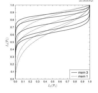
Figure 21: Outer EXIT curves (inverted) of our QIRCC subcodes having code rates $\{1/4,1/3,1/2,2/3,3/4\}$ for both memory-$3$ as well as memory-$1$.

Furthermore, in order to facilitate accurate EXIT curve matching with a sufficiently versatile and diverse set of inner EXIT functions, we also selected $5$ weak randomly-constructed memory-$1$ subcodes for the same range of coding rates, i.e. $\{1/4,1/3,1/2,2/3,3/4\}$. The corresponding seed transformations are as follows:

$$U_{6} =\{475,194,526,422,417,988,426,611,831,84\},$$

$$U_{7} =\{26,147,149,99,112,184,64,139\},$$

$$U_{8} =\{37,55,58,35,57,54\},$$

$$U_{9} =\{57,248,99,226,37,93,244,54\},$$

$$U_{10} =\{469,634,146,70,186,969,387,398,807,452\},$$ (127)

and their EXIT curves are plotted in Fig. 21 with the aid of dotted lines. It must be mentioned here that the range of coding rates chosen for the QIRCC subcodes can be expanded such that the EXIT curves cover a larger portion of the EXIT plot, which further improves curve matching. However, this increases the encoding and decoding complexity.

Based on our proposed QIRCC, relying on the $10$ subcodes specified by Eq. (126) and (127), the input bit stream is divided into $10$ fractions corresponding to the $10$ different-rate subcodes. The specific optimum fractions to be encoded by these codes are found by dynamic programming. More specifically, since the QCCs belong to the class of linear codes, the EXIT curves of the $10$ subcodes, given in Fig. 21, are superimposed onto each other after weighting by the appropriate fraction-based weighting coefficients, which are determined by minimizing the area of the open EXIT-tunnel. To elaborate a little further, the transfer function of the QIRCC is given by the weighted sum of each subcode’s transfer function as shown below:

$$I_{E}(P_{1})=T_{1}[I_{A}(P_{1})]=\sum_{q=1}^{\mathcal{Q}}\varrho_{q}\ T_{1}^{q}\left[I_{A}(P_{1})\right],$$ (128)

where $T_{1}^{q}\left[I_{A}(P_{1})\right]$ is the transfer function of the $q^{th}$ subcode. For a given inner EXIT curve and outer code rate $R_{Q}$, we employ the curve matching algorithm of [115, 114] for optimizing the weighting coefficients $\boldsymbol{\varrho}$ of our proposed QIRCC such that the square of the error between the inner and inverted outer EXIT curves is minimized subject to Eq. (124). More explicitly, the error function may be modeled as:

$$e(i)=T_{2}[i,p]-T_{1}^{-1}[i],$$ (129)

where $p=(p^{*}-\epsilon)$ given that $p^{*}$ is the noise limit defined by the hashing bound and $\epsilon$ is an arbitrarily small number. The corresponding matrix-based notation may be formulated as [115, 114]:

$$\mathbf{e}=\mathbf{b}-\mathbf{A}\boldsymbol{\varrho},$$ (130)

where we have:

$$\mathbf{b} =\begin{pmatrix}T_{2}[i_{1},p]\\ T_{2}[i_{2},p]\\ \vdots\\ T_{2}[i_{\text{N}},p]\end{pmatrix},\text{and}$$

$$\mathbf{A} =\begin{pmatrix}T^{1^{-1}}_{1}[i_{1}]&T^{2^{-1}}_{1}[i_{1}]&\ldots&T^{\mathcal{Q}^{-1}}_{1}[i_{1}]\\ T^{1^{-1}}_{1}[i_{2}]&T^{2^{-1}}_{1}[i_{2}]&\ldots&T^{\mathcal{Q}^{-1}}_{1}[i_{2}]\\ \vdots&\vdots&\vdots&\vdots\\ T^{1^{-1}}_{1}[i_{\text{N}}]&T^{2^{-1}}_{1}[i_{\text{N}}]&\ldots&T^{\mathcal{Q}^{-1}}_{1}[i_{\text{N}}]\end{pmatrix}.$$ (131)

Here, N denotes the number of sample points such that $i\in\{i_{1},i_{2},\dots,i_{\text{N}}\}$ and it is assumed that $\text{N}>\mathcal{Q}$. Furthermore, the error should be greater than zero for the sake of ensuring an open tunnel, i.e. we have:

$$e(i)>0,\ \forall i\in[0,1].$$ (132)

The resultant cost function, i.e. sum of the square of the errors, is given by[115]:

$$\mathcal{J}(\varrho_{1},\dots,\varrho_{\mathcal{Q}})=\int_{0}^{1}e(i)^{2}di,$$ (133)

which may also be written as:

$$\mathcal{J}(\boldsymbol{\varrho})=\mathbf{e}^{T}\mathbf{e}.$$ (134)

The overall process may be encapsulated as follows:

$$\boldsymbol{\varrho}_{opt}=\arg\min_{\boldsymbol{\varrho}}\mathcal{J}(\boldsymbol{\varrho}),$$ (135)

subject to Eq. (124) and (132), which is a convex optimization problem. The unconstrained optimal solution for Eq. (135) is found iteratively using steepest descent approach with a gradient of $\partial\mathcal{J}(\boldsymbol{\varrho})/\partial\boldsymbol{\varrho}=2\mathbf{e}$, which is then projected onto the constraints defined in Eq. (124) and (132). Further details of this optimization algorithm can be found in [115, 114].

VIII Results and Discussions

For the sake of demonstrating the curve matching capability of our proposed QIRCC, we designed a rate-$1/9$ concatenated code relying on the rate-$1/3$ entanglement-assisted inner code of [36, 34], namely “PTO1REA”, with our proposed QIRCC as the outer code. Since the entanglement consumption rate of “PTO1REA” is $2/3$, the resultant code has an entanglement consumption rate of $6/9$, for which the corresponding noise limit is $p^{*}=0.3779$ according to Eq. (5) [34]. Furthermore, since we intend to design a rate-$1/9$ system with a rate-$1/3$ inner code, we have $R_{Q}=1/3$. Hence, for a target coding rate of $1/3$, we used the optimization algorithm discussed in Section VII for the sake of finding the optimum weighting coefficients of Eq. (135) at the highest possible depolarizing probability $p=p^{*}-\epsilon$. It was found that we only need to invoke two subcodes out of the $10$ possible subcodes, based on $\boldsymbol{\varrho}$ = [0 0 0 0 0.168 0.832 0 0 0 0]^T, for attaining a marginally open tunnel, which occurs at $p=0.345$, as shown in Fig. 22. Hence, the resultant code has a convergence threshold of $p=0.345$, which is only $\left[10\times\log_{10}(\frac{0.345}{0.3779})\right]=0.4$ dB from the noise limit of $0.3779$. Fig. 22 also shows two decoding trajectories at $p=0.34$ for a $30,000$ qubit long interleaver. As gleaned from the figure, the decoding trajectories closely follow the EXIT curves reaching the $(1,1)$ point of perfect convergence.

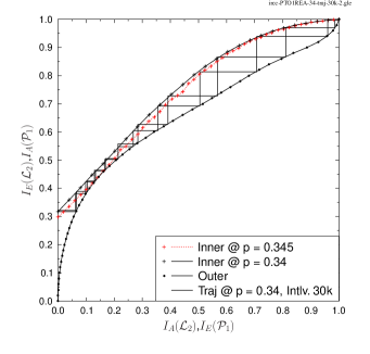
Figure 22: EXIT curves of the concatenated rate-$1/9$ system, with PTO1REA as the inner code and QIRCC as the outer, at $p=0.345$ and $p=0.34$.

The corresponding Word Error Rate (WER) performance curves recorded for our QIRCC-based optimized design using a $3,000$ qubit long interleaver are seen in Fig. 23, where the WER is reduced upon increasing the number of iterations. More explicitly, our code converges to a low WER for $p\leq 0.345$. Thus, this convergence threshold matches the one predicted using EXIT charts in Fig. 22. More explicitly, since the EXIT chart tunnel closes for $p>0.345$, the system fails to converge, if the depolarizing probability is increased beyond $0.345$. Hence, the performance does not improve upon increasing the number of iterations if the depolarizing probability exceeds the threshold. By contrast, when the depolarizing probability is below the threshold, the WER improves at each successive iteration. It should also be noted that the performance improves with diminishing returns at a higher number of iterations.

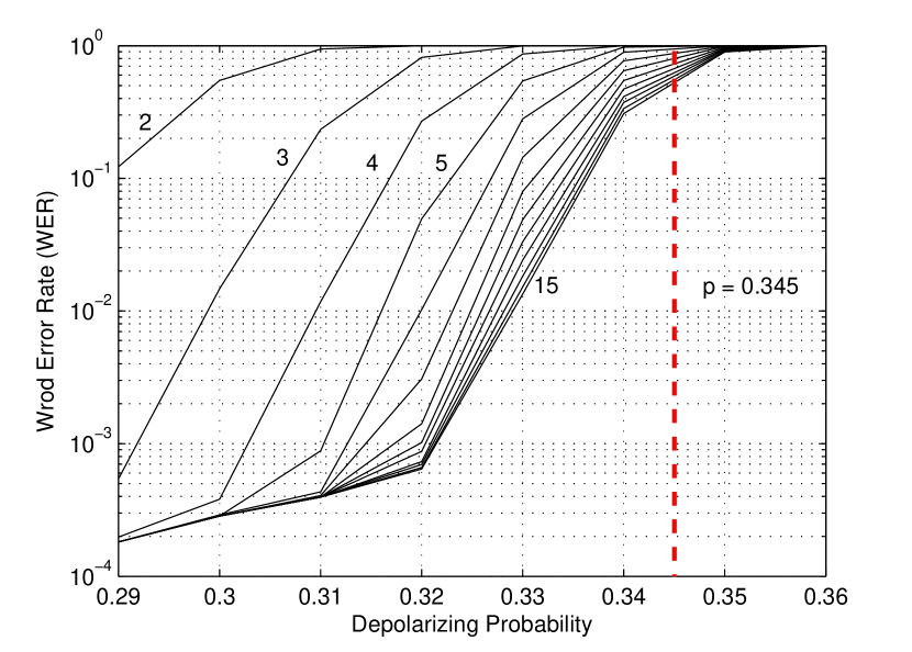
Figure 23: WER performance curves with increasing iteration number for an interleaver length of $3,000$ qubits. Rate-1/9 concatenated code, relying on PTO1REA as the inner code and the proposed QIRCC as the outer code, was used.

Fig. 24 compares our QIRCC-based optimized design with the rate-$1/9$ “PTO1REA-PTO1R” configuration of [34], which is labeled “A” in the figure. An interleaver length of $3000$ qubits was used. For the “PTO1REA-PTO1R” configuration, the turbo cliff region emerges around $0.31$, which is within $0.9$ dB of the noise limit. Therefore, our QIRCC-based design outperforms the “PTO1REA-PTO1R” configuration of [34]. More specifically, the “PTO1REA-PTO1R” configuration yields a WER of $10^{-3}$ at $p=0.29$, while our design gives a WER of $10^{-3}$ at $p=0.322$. Hence, our optimized design outperforms the ‘PTO1REA-PTO1R” configuration by about $\left[10\times\log_{10}(\frac{0.29}{0.322})\right]=0.5$ dB at a WER of $10^{-3}$. It must be mentioned here that the “PTO1REA-PTO1R” configuration may have a lower error floor than our design, yet our design exhibits a better performance in the turbo cliff region. We further compare our QIRCC-based optimized design with the exhaustive-search based optimized turbo code of [35], which is labeled “B” in Fig. 24. Both code designs have similar convergence threshold. However, our QIRCC-based design has a much lower error rate, resulting in a lower error floor as gleaned from Fig. 24.

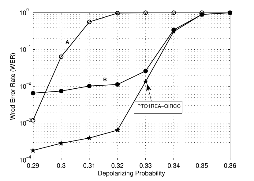
Figure 24: Comparison of WER performance of our QIRCC-based optimized rate-$1/9$ QTC with the PTO1REA-PTO1R configuration of [34] (labeled “A”) and the exhaustive-search based optimized QTC of [35] (labeled “B”) for an interleaver length of $3,000$ qubits and a maximum of $15$ iterations.

IX Conclusions and Design Guidelines

Powerful QECCs are required for stabilizing and protecting the fragile constituent qubits of quantum computation as well as communication systems against the undesirable decoherence. In line with the developments in the field of classical channel coding theory, this may be achieved by exploiting concatenated codes designs, which invoke iterative decoding. Therefore, in this paper we have laid out a slow-paced tutorial for designing hashing bound approaching concatenated quantum codes using EXIT charts. To bridge the gap between the quantum and classical channel coding theory, we have provided insights into the transition from the classical to the quantum code design. More specifically, with the help of toy examples, we have illustrated that quantum block codes as well as convolutional codes may be constructed from arbitrary classical linear codes. We then move onto the construction of concatenated quantum codes, focusing specifically on the circuit-based structure of the constituent encoders and their equivalent classical representation as well as the degenerate iterative decoding. Finally, we have detailed the procedure for generating EXIT charts for quantum codes and the principles of EXIT-chart aided design. Our design guidelines may be summarized as follows:

• As discussed in the context of our design objectives in Section II, we commence our design by determining the noise limit $p^{*}$ for the desired code parameters, i.e the coding rate and the entanglement consumption rate of the resultant concatenated quantum code, which was introduced in Section II.

• We then proceed with the selection of the inner stabilizer code of Fig. 16, which has to be both recursive as well as non-catastrophic, as argued in Section V-B. Since the unassisted quantum codes cannot be simultaneously both recursive as well as non-catastrophic, we employ an entanglement-assisted code. Furthermore, the EA inner code of Fig. 16 may be either derived from the family of known classical codes, as discussed in Section IV or it may be constructed using random Clifford operations, which were discussed in Section V-A. At this point, the EXIT curves of Section VI may be invoked for the sake of finding that specific inner code, which yields the largest area under its EXIT-curve at the noise limit $p^{*}$.

• Finally, we find the optimal non-catastrophic outer code of Fig. 16, which gives the best EXIT-curve match with that of the chosen inner code. In this context, our EXIT-chart aided design of Section VI aims for creating a narrow, but marginally open tunnel between the EXIT curves of the inner and outer decoders at the highest possible depolarizing probability. The narrower the tunnel-area, the lower is the deviation from the hashing bound, which may be quantified using Eq. (4).

Recall that the desired code structure may also be optimized on the basis of a range of conflicting design challenges, which were illustrated in Fig. 4.

Furthermore, for the sake of facilitating the hashing bound approaching code design, we have proposed the structure of QIRCC, which constitutes the outer component of a concatenated quantum code. The proposed QIRCC allows us to dispense with the exhaustive code-search methods, since it can be dynamically adapted to match any given inner code using EXIT charts. We have constructed a $10$-subcode QIRCC and used it as an outer code in concatenation with a non-catastrophic and recursive inner convolutional code of [36, 34]. In contrast to the concatenated codes of [34], whose performance is within $0.9$ dB of the hashing bound, our QIRCC-based optimized design operates within $0.4$ dB of the noise limit. Furthermore, at a WER of $10^{-3}$, our design outperforms the design of [34] by around $0.5$ dB. Our proposed design also yields lower error rate as compared to the exhaustive-search based optimized design of [35].

References

- [1] L. Hanzo, H. Haas, S. Imre, D. O’Brien, M. Rupp, and L. Gyongyosi, “Wireless myths, realities, and futures: From 3G/4G to optical and quantum wireless,” Proceedings of the IEEE, vol. 100, no. Special Centennial Issue, pp. 1853–1888, May 2012.
- [2] P. A. Dirac, The Principles of Quantum Mechanics. Oxford University Press, 1982.
- [3] S. Imre and F. Balazs, Quantum Computing and Communications: An Engineering Approach. John Wiley & Sons, 2005.
- [4] P. Botsinis, S. X. Ng, and L. Hanzo, “Quantum search algorithms, quantum wireless, and a low-complexity maximum likelihood iterative quantum multi-user detector design,” IEEE Access, vol. 1, pp. 94–122, 2013. [Online]. Available: http://ieeexplore.ieee.org/xpl/articleDetails.jsp?arnumber=6515077
- [5] D. Deutsch, “Quantum theory, the church-turing principle and the universal quantum computer,” Proceedings of the Royal Society of London A: Mathematical, Physical and Engineering Sciences, vol. 400, no. 1818, pp. 97–117, 1985.
- [6] D. Deutsch and R. Jozsa, “Rapid solution of problems by quantum computation,” Proceedings of the Royal Society of London A: Mathematical, Physical and Engineering Sciences, vol. 439, no. 1907, pp. 553–558, 1992.
- [7] P. W. Shor, “Algorithms for quantum computation: discrete logarithms and factoring,” in Proceedings of the 35th Annual Symposium on Foundations of Computer Science. Washington, DC, USA: IEEE Computer Society, 1994, pp. 124–134. [Online]. Available: http://portal.acm.org/citation.cfm?id=1398518.1399018
- [8] L. K. Grover, “A fast quantum mechanical algorithm for database search,” in Proceedings of the Twenty-eighth Annual ACM Symposium on Theory of Computing, ser. STOC ’96. New York, NY, USA: ACM, 1996, pp. 212–219. [Online]. Available: http://doi.acm.org/10.1145/237814.237866
- [9] P. Botsinis, S. X. Ng, and L. Hanzo, “Fixed-complexity quantum-assisted multi-user detection for CDMA and SDMA,” IEEE Transactions on Communications, vol. 62, no. 3, pp. 990–1000, March 2014.
- [10] P. Botsinis, D. Alanis, S. Ng, and L. Hanzo, “Low-complexity soft-output quantum-assisted multiuser detection for direct-sequence spreading and slow subcarrier-hopping aided SDMA-OFDM systems,” IEEE Access, vol. 2, pp. 451–472, 2014.
- [11] D. Alanis, P. Botsinis, S. X. Ng, and L. Hanzo, “Quantum-assisted routing optimization for self-organizing networks,” IEEE Access, vol. 2, pp. 614–632, 2014.
- [12] M. Born, The Born-Einstein letters. Walker, 1971.
- [13] M. A. Nielsen and I. L. Chuang, Quantum Computation and Quantum Information. Cambridge University Press, 2000.
- [14] S. Wiesner, “Conjugate coding,” SIGACT News, vol. 15, pp. 78–88, January 1983. [Online]. Available: http://doi.acm.org/10.1145/1008908.1008920
- [15] C. H. Bennett and G. Brassard, “Quantum cryptography: public key distribution and coin tossing,” in Proceedings of the IEEE International Conference on Computers, Systems and Signal Processing. New York: IEEE Press, 1984, pp. 175–179.
- [16] A. Beige, B.-G. Englert, C. Kurtsiefer, and H. Weinfurter, “Secure communication with single-photon two-qubit states,” Journal of Physics A: Mathematical and General, vol. 35, no. 28, p. L407, Jul 2002. [Online]. Available: http://stacks.iop.org/0305-4470/35/i=28/a=103
- [17] K. Boström and T. Felbinger, “Deterministic secure direct communication using entanglement,” Phys. Rev. Lett., vol. 89, p. 187902, Oct 2002. [Online]. Available: http://link.aps.org/doi/10.1103/PhysRevLett.89.187902
- [18] R. A. Malaney, “Location-dependent communications using quantum entanglement,” Phys. Rev. A, vol. 81, p. 042319, Apr 2010. [Online]. Available: http://link.aps.org/doi/10.1103/PhysRevA.81.042319
- [19] P. W. Shor, “Scheme for reducing decoherence in quantum computer memory,” Physical Review A, vol. 52, no. 4, pp. R2493–R2496, Oct. 1995. [Online]. Available: http://dx.doi.org/10.1103/PhysRevA.52.R2493
- [20] J. Preskill, “Battling decoherence: the fault-tolerant quantum computer,” Physics Today, vol. 52, pp. 24–32, 1999.
- [21] ——, “Reliable quantum computers,” in Proc. Royal Soc. of London A, vol. 454, 1998, pp. 385–410.
- [22] M. M. Wilde, Quantum Information Theory. Cambridge University Press, May 2013. [Online]. Available: http://arxiv.org/abs/1106.1445
- [23] D. G. Cory, M. D. Price, W. Maas, E. Knill, R. Laflamme, W. H. Zurek, T. F. Havel, and S. S. Somaroo, “Experimental quantum error correction,” Phys. Rev. Lett., vol. 81, pp. 2152–2155, Sep 1998. [Online]. Available: http://link.aps.org/doi/10.1103/PhysRevLett.81.2152
- [24] M. D. Reed, L. DiCarlo, S. E. Nigg, L. Sun, L. Frunzio, S. M. Girvin, and R. J. Schoelkopf, “Realization of three-qubit quantum error correction with superconducting circuits,” Nature, vol. 482, no. 7385, pp. 382–385, Feb. 2012. [Online]. Available: http://dx.doi.org/10.1038/nature10786
- [25] G. Arrad, Y. Vinkler, D. Aharonov, and A. Retzker, “Increasing sensing resolution with error correction,” Phys. Rev. Lett., vol. 112, p. 150801, Apr 2014. [Online]. Available: http://link.aps.org/doi/10.1103/PhysRevLett.112.150801
- [26] S. Lin and D. J. Costello, Error Control Coding. New Jersey, USA: Pearson-Prentice Hall, 2004.
- [27] L. Hanzo, T. H. Liew, B. L. Yeap, R. Y. S. Tee and S. X. Ng, Turbo Coding, Turbo Equalisation and Space-Time Coding: EXIT-Chart-Aided Near-Capacity Designs for Wireless Channels, 2nd Edition. New York, USA: John Wiley IEEE Press, March 2011.
- [28] S. Lloyd, “Capacity of the noisy quantum channel,” Phys. Rev. A, vol. 55, pp. 1613–1622, Mar 1997. [Online]. Available: http://link.aps.org/doi/10.1103/PhysRevA.55.1613
- [29] P. W. Shor, “The quantum channel capacity and coherent information,” Lecture Notes, MSRI Workshop on Quantum Computation, 2002.
- [30] I. Devetak, “The private classical capacity and quantum capacity of a quantum channel,” IEEE Transactions on Information Theory, vol. 51, no. 1, pp. 44–55, Jan 2005.
- [31] C. Berrou, A. Glavieux, and P. Thitimajshima, “Near Shannon limit error-correcting coding and decoding: Turbo-codes. 1,” in Technical Program of the IEEE International Conference on Communications, ICC ’93 Geneva, vol. 2, May 1993, pp. 1064–1070 vol.2.
- [32] S. ten Brink, “Convergence behaviour of iteratively decoded parallel concatenated codes,” IEEE Transactions on Communications, vol. 49, no. 10, pp. 1727–1737, October 2001.
- [33] D. Poulin, J. Tillich, and H. Ollivier, “Quantum serial turbo codes,” IEEE Transactions on Information Theory, vol. 55, no. 6, pp. 2776–2798, June 2009.
- [34] M. Wilde, M.-H. Hsieh, and Z. Babar, “Entanglement-assisted quantum turbo codes,” IEEE Transactions on Information Theory, vol. 60, no. 2, pp. 1203–1222, Feb 2014.
- [35] Z. Babar, S. X. Ng, and L. Hanzo, “EXIT-chart aided near-capacity quantum turbo code design,” IEEE Transactions on Vehicular Technology, vol. PP, no. 99, pp. 1–1, 2014.
- [36] M. M. Wilde and M.-H. Hsieh, “Entanglement boosts quantum turbo codes,” in IEEE International Symposium on Information Theory, Aug. 2011, pp. 445 – 449.
- [37] W. K. Wootters and W. H. Zurek, “A single quantum cannot be cloned,” Nature, vol. 299, no. 5886, pp. 802–803, Oct. 1982. [Online]. Available: http://dx.doi.org/10.1038/299802a0
- [38] D. MacKay, G. Mitchison, and P. McFadden, “Sparse-graph codes for quantum error correction,” IEEE Transactions on Information Theory, vol. 50, no. 10, pp. 2315–2330, Oct 2004.
- [39] D. Poulin, J.-P. Tillich, and H. Ollivier, “Quantum serial turbo-codes,” in IEEE International Symposium on Information Theory, July 2008, pp. 310–314.
- [40] J. M. Renes, F. Dupuis, and R. Renner, “Efficient polar coding of quantum information,” Phys. Rev. Lett., vol. 109, p. 050504, Aug 2012. [Online]. Available: http://link.aps.org/doi/10.1103/PhysRevLett.109.050504
- [41] D. P. DiVincenzo, P. W. Shor, and J. A. Smolin, “Quantum-channel capacity of very noisy channels,” Phys. Rev. A, vol. 57, pp. 830–839, Feb 1998. [Online]. Available: http://link.aps.org/doi/10.1103/PhysRevA.57.830
- [42] G. Smith and J. A. Smolin, “Degenerate quantum codes for pauli channels,” Phys. Rev. Lett., vol. 98, p. 030501, Jan 2007. [Online]. Available: http://link.aps.org/doi/10.1103/PhysRevLett.98.030501
- [43] C. H. Bennett, D. P. DiVincenzo, J. A. Smolin, and W. K. Wootters, “Mixed-state entanglement and quantum error correction,” Phys. Rev. A, vol. 54, pp. 3824–3851, Nov 1996. [Online]. Available: http://link.aps.org/doi/10.1103/PhysRevA.54.3824
- [44] G. Bowen, “Entanglement required in achieving entanglement-assisted channel capacities,” Phys. Rev. A, vol. 66, p. 052313, Nov 2002. [Online]. Available: http://link.aps.org/doi/10.1103/PhysRevA.66.052313
- [45] T. A. Brun, I. Devetak, and M.-H. Hsieh, “Correcting quantum errors with entanglement,” Science, vol. 314, no. 5798, oct. 2006.
- [46] ——, “General entanglement-assisted quantum error-correcting codes,” in IEEE International Symposium on Information Theory, june 2007, pp. 2101 –2105.
- [47] M.-H. Hsieh, I. Devetak, and T. Brun, “General entanglement-assisted quantum error-correcting codes,” Phys. Rev. A, vol. 76, p. 062313, Dec 2007. [Online]. Available: http://link.aps.org/doi/10.1103/PhysRevA.76.062313
- [48] C.-Y. Lai, T. Brun, and M. Wilde, “Dualities and identities for entanglement-assisted quantum codes,” Quantum Information Processing, vol. 13, no. 4, pp. 957–990, 2014. [Online]. Available: http://dx.doi.org/10.1007/s11128-013-0704-8
- [49] A. R. Calderbank and P. W. Shor, “Good quantum error-correcting codes exist,” Phys. Rev. A, vol. 54, no. 2, pp. 1098–1105, Aug 1996.
- [50] A. Steane, “Multiple-particle interference and quantum error correction,” Royal Society of London Proceedings Series A, vol. 452, pp. 2551–2577, Nov. 1995.
- [51] A. M. Steane, “Error correcting codes in quantum theory,” Phys. Rev. Lett., vol. 77, no. 5, pp. 793–797, Jul 1996.
- [52] R. Laflamme, C. Miquel, J. P. Paz, and W. H. Zurek, “Perfect quantum error correcting code,” Phys. Rev. Lett., vol. 77, pp. 198–201, Jul 1996. [Online]. Available: http://link.aps.org/doi/10.1103/PhysRevLett.77.198
- [53] D. Gottesman, “Class of quantum error-correcting codes saturating the quantum Hamming bound,” Phys. Rev. A, vol. 54, no. 3, pp. 1862–1868, Sep 1996.
- [54] ——, “Stabilizer codes and quantum error correction,” Ph.D. dissertation, California Institute of Technology, 1997.
- [55] M. Grassl, T. Beth, and T. Pellizzari, “Codes for the quantum erasure channel,” Phys. Rev. A, vol. 56, pp. 33–38, Jul 1997. [Online]. Available: http://link.aps.org/doi/10.1103/PhysRevA.56.33
- [56] A. Calderbank, E. Rains, P. Shor, and N. J. A. Sloane, “Quantum error correction via codes over GF(4),” IEEE Transactions on Information Theory, vol. 44, no. 4, pp. 1369–1387, Jul 1998.
- [57] M. Grassl and T. Beth, “Quantum BCH Codes,” Proceedings of International Symposium on Theoretical Electrical Engineering Magdeburg, pp. 207–212, Oct. 1999. [Online]. Available: http://arxiv.org/abs/quant-ph/9910060
- [58] A. Steane, “Enlargement of Calderbank-Shor-Steane quantum codes,” IEEE Transactions on Information Theory, vol. 45, no. 7, pp. 2492–2495, Nov 1999.
- [59] ——, “Quantum Reed-Muller codes,” IEEE Transactions on Information Theory, vol. 45, no. 5, pp. 1701–1703, Jul 1999.
- [60] M. Grassl, W. Geiselmann, and T. Beth, “Quantum Reed-Solomon codes,” in Proceedings Applied Algebra, Algebraic Algorithms and Error-Correcting Codes (AAECC-13). Springer. See, 1999, pp. 231–244.
- [61] M. S. Postol, “A proposed quantum low density parity check code,” arXiv:quant-ph/0108131v1, 2001.
- [62] T. Camara, H. Ollivier, and J.-P. Tillich, “Constructions and performance of classes of quantum LDPC codes,” arXiv:quant-ph/0502086v2, 2005.
- [63] ——, “A class of quantum LDPC codes: construction and performances under iterative decoding,” in IEEE International Symposium on Information Theory, June 2007, pp. 811–815.
- [64] H. Ollivier and J.-P. Tillich, “Description of a quantum convolutional code,” Phys. Rev. Lett., vol. 91, p. 177902, Oct 2003. [Online]. Available: http://link.aps.org/doi/10.1103/PhysRevLett.91.177902
- [65] H. Ollivier and J. P. Tillich, “Quantum convolutional codes: fundamentals,” quant-ph/0401134, 2004.
- [66] G. Forney and S. Guha, “Simple rate-1/3 convolutional and tail-biting quantum error-correcting codes,” in IEEE International Symposium on Information Theory, Sept. 2005, pp. 1028 –1032.
- [67] G. D. Forney, M. Grassl, and S. Guha, “Convolutional and tail-biting quantum error-correcting codes,” IEEE Transactions on Information Theory, vol. 53, no. 3, pp. 865–880, March 2007.
- [68] M. Wilde and S. Guha, “Polar codes for degradable quantum channels,” IEEE Transactions on Information Theory, vol. 59, no. 7, pp. 4718–4729, July 2013.
- [69] J. Renes and M. Wilde, “Polar codes for private and quantum communication over arbitrary channels,” IEEE Transactions on Information Theory, vol. 60, no. 6, pp. 3090–3103, June 2014.
- [70] P. Piret, Convolutional Codes: An Algebraic Approach. MIT Press, Cambridge, MA, 1988.
- [71] H. F. Chau, “Quantum convolutional error-correcting codes,” Phys. Rev. A, vol. 58, pp. 905–909, Aug 1998. [Online]. Available: http://link.aps.org/doi/10.1103/PhysRevA.58.905
- [72] ——, “Good quantum-convolutional error-correction codes and their decoding algorithm exist,” Phys. Rev. A, vol. 60, pp. 1966–1974, Sep 1999. [Online]. Available: http://link.aps.org/doi/10.1103/PhysRevA.60.1966
- [73] A. Aido De Almeida and J. Palazzo, R., “A concatenated [(4, 1, 3)] quantum convolutional code,” in IEEE Information Theory Workshop, Oct. 2004, pp. 28 – 33.
- [74] M. Grassl and M. Rotteler, “Quantum block and convolutional codes from self-orthogonal product codes,” in IEEE International Symposium on Information Theory, Sep. 2005, pp. 1018 –1022.
- [75] ——, “Constructions of quantum convolutional codes,” in IEEE International Symposium on Information Theory, June 2007, pp. 816–820.
- [76] S. Aly, M. Grassl, A. Klappenecker, M. Rotteler, and P. Sarvepalli, “Quantum convolutional BCH codes,” in 10th Canadian Workshop on Information Theory, June 2007, pp. 180 –183.
- [77] S. A. Aly, A. Klappenecker, and P. K. Sarvepalli, “Quantum convolutional codes derived from generalized Reed-Solomon codes,” in IEEE International Symposium on Information Theory, June 2007, pp. 821 –825.
- [78] E. Pelchat and D. Poulin, “Degenerate Viterbi decoding,” IEEE Transactions on Information Theory, vol. 59, no. 6, pp. 3915–3921, 2013.
- [79] R. Gallager, “Low-density parity-check codes,” IRE Transactions on Information Theory, vol. 8, no. 1, pp. 21–28, January 1962.
- [80] D. Mackay, G. Mitchison, and A. Shokrollahi, “More sparse-graph codes for quantum error-correction,” www.inference.phy.cam.ac.uk/mackay/cayley.pdf, 2007.
- [81] A. Couvreur, N. Delfosse, and G. Zemor, “A construction of quantum LDPC codes from cayley graphs,” in IEEE International Symposium on Information Theory, 31 2011-aug. 5 2011, pp. 643 –647.
- [82] ——, “A construction of quantum LDPC codes from cayley graphs,” IEEE Transactions on Information Theory, vol. 59, no. 9, pp. 6087–6098, Sept 2013.
- [83] S. Aly, “A class of quantum LDPC codes constructed from finite geometries,” in IEEE Global Telecommunications Conference, 30 2008-dec. 4 2008, pp. 1 –5.
- [84] I. Djordjevic, “Quantum LDPC codes from balanced incomplete block designs,” IEEE Communications Letters, vol. 12, no. 5, pp. 389 –391, may 2008.
- [85] H. Lou and J. Garcia-Frias, “Quantum error-correction using codes with low-density generator matrix,” in IEEE 6th Workshop on Signal Processing Advances in Wireless Communications, june 2005, pp. 1043 – 1047.
- [86] ——, “On the application of error-correcting codes with low-density generator matrix over different quantum channels,” International ITG-Conference on Source and Channel Coding, pp. 1 –6, april 2006.
- [87] M. Hagiwara and H. Imai, “Quantum quasi-cyclic LDPC codes,” in IEEE International Symposium on Information Theory, june 2007, pp. 806 –810.
- [88] K. Kasai, M. Hagiwara, H. Imai, and K. Sakaniwa, “Non-binary quasi-cyclic quantum LDPC codes,” in IEEE International Symposium on Information Theory, 31 2011-aug. 5 2011, pp. 653 –657.
- [89] ——, “Quantum error correction beyond the bounded distance decoding limit,” IEEE Transactions on Information Theory, vol. 58, no. 2, pp. 1223 –1230, feb. 2012.
- [90] M. Hagiwara, K. Kasai, H. Imai, and K. Sakaniwa, “Spatially coupled quasi-cyclic quantum LDPC codes,” in IEEE International Symposium on Information Theory, 31 2011-aug. 5 2011, pp. 638 –642.
- [91] P. Tan and J. Li, “Efficient quantum stabilizer codes: LDPC and LDPC-convolutional constructions,” IEEE Transactions on Information Theory, vol. 56, no. 1, pp. 476 –491, jan. 2010.
- [92] N. Delfosse, “Tradeoffs for reliable quantum information storage in surface codes and color codes,” in IEEE International Symposium on Information Theory, July 2013, pp. 917–921.
- [93] A. A. Kovalev and L. P. Pryadko, “Quantum Kronecker sum-product low-density parity-check codes with finite rate,” Phys. Rev. A, vol. 88, p. 012311, Jul 2013. [Online]. Available: http://link.aps.org/doi/10.1103/PhysRevA.88.012311
- [94] J.-P. Tillich and G. Zemor, “Quantum LDPC codes with positive rate and minimum distance proportional to the square root of the blocklength,” IEEE Transactions on Information Theory, vol. 60, no. 2, pp. 1193–1202, Feb 2014.
- [95] D. Poulin and Y. Chung, “On the iterative decoding of sparse quantum codes,” Quantum Info. Comput., vol. 8, no. 10, pp. 987–1000, Nov. 2008. [Online]. Available: http://dl.acm.org/citation.cfm?id=2016985.2016993
- [96] Y.-J. Wang, B. Sanders, B.-M. Bai, and X.-M. Wang, “Enhanced feedback iterative decoding of sparse quantum codes,” IEEE Transactions on Information Theory, vol. 58, no. 2, pp. 1231 –1241, feb. 2012.
- [97] J. Kliewer, S. X. Ng, and L. Hanzo, “Efficient computation of EXIT functions for non-binary iterative decoding,” IEEE Transactions on Communications, vol. 54, no. 12, pp. 2133–2136, December 2006.
- [98] M. Houshmand and M. Wilde, “Recursive quantum convolutional encoders are catastrophic: A simple proof,” IEEE Transactions on Information Theory, vol. 59, no. 10, pp. 6724–6731, 2013.
- [99] M.-H. Hsieh, T. A. Brun, and I. Devetak, “Entanglement-assisted quantum quasicyclic low-density parity-check codes,” Phys. Rev. A, vol. 79, p. 032340, Mar 2009. [Online]. Available: http://link.aps.org/doi/10.1103/PhysRevA.79.032340
- [100] M. M. Wilde and T. A. Brun, “Entanglement-assisted quantum convolutional coding,” Phys. Rev. A, vol. 81, p. 042333, Apr 2010. [Online]. Available: http://link.aps.org/doi/10.1103/PhysRevA.81.042333
- [101] M. Wilde and J. Renes, “Quantum polar codes for arbitrary channels,” in IEEE International Symposium on Information Theory, july 2012, pp. 334 –338.
- [102] Z. Babar, S. X. Ng, and L. Hanzo, “Reduced-complexity syndrome-based TTCM decoding,” IEEE Communications Letters, vol. 17, no. 6, pp. 1220–1223, 2013.
- [103] R. Cleve, “Quantum stabilizer codes and classical linear codes,” Phys. Rev. A, vol. 55, pp. 4054–4059, Jun 1997. [Online]. Available: http://link.aps.org/doi/10.1103/PhysRevA.55.4054
- [104] C. H. Bennett, “Communication via one- and two-particle operators on Einstein-Podolsky-Rosen states,” Physical Review Letters, vol. 69, no. 20, p. 2881, 1992. [Online]. Available: http://dx.doi.org/%7B10.1103/PhysRevLett.69.2881%7D
- [105] J. Dehaene and B. De Moor, “Clifford group, stabilizer states, and linear and quadratic operations over GF(2),” Phys. Rev. A, vol. 68, p. 042318, Oct 2003. [Online]. Available: http://link.aps.org/doi/10.1103/PhysRevA.68.042318
- [106] D. Gottesman, The Heisenberg Representation of Quantum Computers. [online] http://arxiv.org/pdf/quant-ph/9807006v1.pdf, December 2001.
- [107] M. El-Hajjar and L. Hanzo, “EXIT charts for system design and analysis,” IEEE Communications Surveys Tutorials, vol. 16, no. 1, pp. 127–153, First 2014.
- [108] S. Ten Brink, “Rate one-half code for approaching the Shannon limit by 0.1 dB,” Electronics Letters, vol. 36, no. 15, pp. 1293–1294, 2000.
- [109] L. Kong, S. X. Ng, R. Maunder, and L. Hanzo, “Maximum-throughput irregular distributed space-time code for near-capacity cooperative communications,” IEEE Transactions on Vehicular Technology, vol. 59, no. 3, pp. 1511–1517, 2010.
- [110] S. Ibi, T. Matsumoto, R. Thoma, S. Sampei, and N. Morinaga, “EXIT chart-aided adaptive coding for multilevel BICM with turbo equalization in frequency-selective MIMO channels,” IEEE Transactions on Vehicular Technology, vol. 56, no. 6, pp. 3757–3769, 2007.
- [111] Z. Babar, S. X. Ng, and L. Hanzo, “Near-capacity code design for entanglement-assisted classical communication over quantum depolarizing channels,” IEEE Transactions on Communications, vol. 61, no. 12, pp. 4801–4807, December 2013.
- [112] A. Grant, “Convergence of non-binary iterative decoding,” in IEEE Global Telecommunications Conference, vol. 2, 2001, pp. 1058–1062 vol.2.
- [113] S. X. Ng, O. Alamri, Y. Li, J. Kliewer, and L. Hanzo, “Near-capacity turbo trellis coded modulation design based on EXIT charts and union bounds,” IEEE Transactions on Communications, vol. 56, no. 12, pp. 2030 –2039, December 2008.
- [114] M. Tüchler, “Design of serially concatenated systems depending on the block length,” IEEE Transactions on Communications, vol. 52, no. 2, pp. 209–218, February 2004.
- [115] M. Tüchler and J. Hagenauer, “EXIT charts of irregular codes,” in Proceedings of Conference on Information Science and Systems, Princeton University, 20-22 March 2002, pp. 748–753.
- [116] E. Rains, “Nonbinary quantum codes,” IEEE Transactions on Information Theory, vol. 45, no. 6, pp. 1827–1832, 1999.
- [117] D. P. Divincenzo, D. Leung, and B. Terhal, “Quantum data hiding,” IEEE Transactions on Information Theory, vol. 48, no. 3, pp. 580–598, Mar 2002.