Vulnerability Analysis of Power Systems

Abstract

Potential vulnerabilities in a power grid can be exposed by identifying those transmission lines on which attacks (in the form of interference with their transmission capabilities) causes maximum disruption to the grid. In this study, we model the grid by (nonlinear) AC power flow equations, and assume that attacks take the form of increased impedance along transmission lines. We quantify disruption in several different ways, including (a) overall deviation of the voltages at the buses from $\displaystyle 1.0$ per unit (p.u.), and (b) the minimal amount of load that must be shed in order to restore the grid to stable operation. We describe optimization formulations of the problem of finding the most disruptive attack, which are either nonlinear programing problems or nonlinear bilevel optimization problems, and describe customized algorithms for solving these problems. Experimental results on the IEEE 118-Bus system and a Polish 2383-Bus system are presented.

I Introduction

Identifying the vulnerable components in a power grid is vital to the design and operation of a secure, stable system. One aspect of vulnerability analysis is to identify those transmission lines for which minor perturbations in their conductive properties leads to major disruptions to the grid, such as voltage drops, or the need for load shedding at demand nodes to restore feasible operation.

Vulnerability assessment for power systems has been widely studied in recent times. Most works focus on minimizing the costs of load shedding and additional generation in the DC model (which is relatively easy to solve) or in lossless AC models (still relatively easy to solve and analyze). In [1, 2, 3], identification of critical components of a power system is formulated in a mixed-integer bilevel programming framework, and attacks on different types of system components (transmission lines, generators, and transformers) are considered. The lower-level problem in the bilevel formulation is replaced by its dual in [2] and is approximated using KKT conditions in [3]. As an extension of [1], an approach based on Bender’s decomposition is proposed to solve larger instances of the transmission line attack problem in [4].

Vulnerability assessment using the lossless AC model is studied in [5, 6]. In these papers, transmission-line attacks are formulated as bilevel optimization problems, in which either unmet demands are maximized or attack costs (number of lines to attack) are minimized to meet a specified level of grid disruption. (These models are also discussed in [7], which describes the equivalence of the two models.) Then the lower-level problem is replaced by its KKT conditions, yielding the single-level optimization problem that is actually solved. In [5], this mixed-integer problem is relaxed to a continuous problem (the binary variables are relaxed to real variables confined to the interval $\displaystyle[0,1]$), while [6] develops a graph-partitioning approach by identifying load-rich and generation-rich regions.

The paper [8] describes a model that uses both load shedding and line switching as defensive operations to reduce the disruption of the system; the model is solved via Bender’s decomposition with a restart framework. Use of a genetic algorithm to solve the “$\displaystyle N-k$” problem (identifying the set of $\displaystyle k$ lines in a grid of $\displaystyle N$ lines whose removal causes maximum disruption) is discussed in [9]. A minimum-cardinality approach (solved using a cutting-plane method) and a continuous nonlinear attack model employing the DC power flow to represent power grids, where a fictitious adversary modifies reactances, are applied to the “$\displaystyle N-k$” problem in [10].

In this paper, we propose two optimization models for vulnerability analysis. Both models are founded on the AC power flow equations, and both consider attacks in which the impedances of transmission lines are increased. In both formulations, the attacks respect a certain “budget;” their total amount of impedance adjustment cannot exceed a certain specified level. The goal of the attacks is to maximize disruption, as measured by two different metrics.

The first metric quantifies voltage disturbance at the buses, leading to a nonlinear programming formulation. The voltage disturbance usually appears as voltage drop, which often leads to an undesirable situation where voltages become low enough that the system cannot maintain stability. This situation, which is called voltage collapse or voltage instability, can happen either quickly or relatively slowly, and is characterized by a parallel process where reactive power demand correspondingly increases. This eventuality causes the active-power behavior of the system to approach the ”nose” of the $\displaystyle P-V$ curve. A more complete description is provided in [11, pages 31 and 35]. With our first metric, we estimate this possible voltage instability of a power grid assuming there is no response from a system operator to the attack.

The second metric we consider here is a weighted sum of the amount of load shedding (at demand nodes) and generation reduction (at generation nodes) that is required to restore feasible operation of the grid following the attack. This power adjustment is considered as a defensive action of a system operator to keep voltages within a stable range to avoid voltage collapse. This case is modeled as a bilevel optimization problem, in which the lower level finds the minimum load adjustment required to respond to the attack, and the upper-level problem is to find the most disruptive attack.

In some existing literature, including some of the papers cited above, a bilevel optimization model is reformulated as a single-level optimization problem by replacing the lower level problem by its optimality conditions. This formulation strategy is unappealing, as the optimality conditions characterize only a stationary point, rather than a minimizer, so they may allow consideration of saddle points or local maximizers. In addition, if the bilevel formulation is designed to solve the attacker-defender framework that we consider in this paper, the reformulated single-level optimization model constructed by replacing the lower-level problem by primal-dual optimality conditions has the serious flaw that the model may exclude the most effective attack. Specifically, an attack (upper level decision) that leads to an infeasible lower level problem obviously maximizes the disruption and thus is “optimal” for the attack problem (since it is not possible to make a operational decision at the lower level to defend against the attack). However, such an attack is excluded from consideration by the single-level reformulation since no (lower-level) primal-dual point satisfies the optimality condition constraints under the attack. Thus, the single-level formulation will ignore the most critical attack. Another drawback of single-level reformulations is that the optimality-condition constraints may violate constraint qualifications, causing possible complications in convergence behavior.

The main contributions of this paper can be summarized as follows:

1. In contrast to previous attack models, the grid is modeled with full AC power flow equations, which are the most accurate mathematical models of power flow.

2. In our bilevel optimization formulation, we actually solve the lower-level problem rather than replacing it by its optimality conditions, as is done in earlier works, to avoid the formulation defects discussed above.

3. We develop effective heuristics that make our formulations tractable even for power grids with thousands of buses.

The remaining sections are organized as follows. We develop the optimization models in Section II and describe the challenges to be addressed in solving them. Section III describes heuristics and optimization techniques that address these challenges and that yield solutions of the problems. Experimental results on 118-Bus and 2383-Bus cases are presented in Section IV, and we discuss conclusions in Section V.

II Problem Description

In this section we discuss power systems background and notation, and describe our two formulations of the vulnerability analysis problem. We describe notation and background on power flow equations in Subsection II-A. Our first vulnerability model, based on a voltage disturbance objective, is discussed in Subsection II-B. The second model, based on a power-adjustment criterion, is discussed in Subsection II-C.

II-A Notations and Background

We summarize here the power systems notation used in later sections, most of which is standard.

• Set of buses: $\displaystyle{\cal N}$

• Set of generators: $\displaystyle{\cal G}\subseteq{\cal N}$

• Set of demand buses: $\displaystyle{\cal D}\subseteq{\cal N}$

• Index of the slack bus: $\displaystyle s\in{\cal N}$

• Set of transmission lines: $\displaystyle{\cal L}\subseteq{\cal N}\times{\cal N}$

• Unit imaginary number: $\displaystyle j=\sqrt{-1}$

• Complex power at bus $\displaystyle i\in{\cal N}$: $\displaystyle P_{i}+jQ_{i}$ (active power: $\displaystyle P_{i}$; real power: $\displaystyle Q_{i}$)

• Complex voltage at bus $\displaystyle i\in{\cal N}$: $\displaystyle V_{i}e^{j\theta_{i}}$ (voltage magnitude: $\displaystyle V_{i}$; phase angle: $\displaystyle\theta_{i}$)

• Difference of angles $\displaystyle\theta_{i}$ and $\displaystyle\theta_{i^{\prime}}$, for $\displaystyle(i,i^{\prime})\in{\cal L}$: $\displaystyle\theta_{ii^{\prime}}:=\theta_{i}-\theta_{i^{\prime}}$

• $\displaystyle(i,i^{\prime})$ entry of the admittance matrix for the (unperturbed) grid: $\displaystyle G_{ii^{\prime}}+jB_{ii^{\prime}}$ (conductance: $\displaystyle G_{ii^{\prime}}$; susceptance: $\displaystyle B_{ii^{\prime}}$).

We assume that the set of generators $\displaystyle{\cal G}$ and the set of demand buses $\displaystyle{\cal D}$ form a partition of $\displaystyle{\cal N}$.

An attack on the grid is specified by means of a line perturbation vector: $\displaystyle\gamma\in{\mathbb{R}}_{+}^{|{\cal L}|}$, with $\displaystyle\gamma_{ii^{\prime}}$ denoting the relative increase in impedance on line $\displaystyle(i,i^{\prime})\in{\cal L}$. Specifically, an attack designated by the vector $\displaystyle\gamma$ causes conductances and susceptances to be modified as follows:

$$\displaystyle G_{ii^{\prime}}(\gamma) \displaystyle=\begin{cases}\frac{G_{ii^{\prime}}}{\gamma_{ii^{\prime}}+1}&\text{if }i\neq i^{\prime},\\ -\sum_{i\neq m}G_{im}(\gamma)&\text{if }i=i^{\prime},\end{cases}$$

$$\displaystyle B_{ii^{\prime}}(\gamma) \displaystyle=\begin{cases}\frac{B_{ii^{\prime}}}{\gamma_{ii^{\prime}}+1}&\text{if }i\neq i^{\prime},\\ -\sum_{i\neq m}\left(B_{im}(\gamma)-\frac{1}{2}B_{im}^{sh}\right)&\text{if }i=i^{\prime},\end{cases}$$

where $\displaystyle B_{im}^{sh}$ is the shunt (line charging) admittance of line $\displaystyle(i,m)\in{\cal L}$. More details on the bus admittance matrix can be found from [12, Chapter 9]. Note that when $\displaystyle\gamma_{ii^{\prime}}=0$ for all $\displaystyle(i,i^{\prime})\in{\cal L}$, the conductances and susceptances all attain their original (unperturbed) values.

The AC power flow equations with perturbations $\displaystyle\gamma$ can be written as follows:

$$\begin{bmatrix}F^{P}(V,\theta;\gamma)\\ F^{Q}(V,\theta;\gamma)\end{bmatrix}\,=\,0,$$ (1)

where the entries of $\displaystyle F^{P}$ and $\displaystyle F^{Q}$ (for all $\displaystyle i\in{\cal N}$) are defined as follows, for all $\displaystyle i\in{\cal N}$:

$$\displaystyle\begin{split}F^{P}_{i}(&V,\theta;\gamma)\,:=\\ &V_{i}\sum_{\mathclap{i^{\prime}:(i,i^{\prime})\in{\cal L}}}V_{i^{\prime}}(G_{ii^{\prime}}(\gamma)\cos{\theta_{ii^{\prime}}}+B_{ii^{\prime}}(\gamma)\sin{\theta_{ii^{\prime}}})-P_{i},\end{split}$$ (2a)

$$\displaystyle\begin{split}F^{Q}_{i}(&V,\theta;\gamma)\,:=\\ &V_{i}\sum_{\mathclap{i^{\prime}:(i,i^{\prime})\in{\cal L}}}V_{i^{\prime}}(G_{ii^{\prime}}(\gamma)\sin{\theta_{ii^{\prime}}}-B_{ii^{\prime}}(\gamma)\cos{\theta_{ii^{\prime}}})-Q_{i}.\end{split}$$ (2b)

We assume throughout the paper that $\displaystyle P_{i}>0$ for generator buses $\displaystyle i\in{\cal G}$ and $\displaystyle P_{i}<0$ and $\displaystyle Q_{i}<0$ for demand buses $\displaystyle i\in{\cal D}$. The power flow problem is to find the values of the vectors $\displaystyle V$, $\displaystyle\theta$, $\displaystyle P$, and $\displaystyle Q$ that satisfy equations (2), given the load demands $\displaystyle P_{\cal D}$ and $\displaystyle Q_{\cal D}$ at load buses and the voltage magnitudes $\displaystyle V_{\cal G}$ and active power injection $\displaystyle P_{\cal G}$ at the generator buses. Conventionally, the reactive powers $\displaystyle Q_{{\cal G}}$ are eliminated from the problem (since they can be obtained explicitly from (2b) for $\displaystyle i\in{\cal G}$, and appear in no other equations), yielding the following reduced formulation:

$$F(V,\theta;\gamma)\,=\,\begin{bmatrix}F_{\cal G}^{P}(V,\theta;\gamma)\\ F_{\cal D}^{P}(V,\theta;\gamma)\\ F_{\cal D}^{Q}(V,\theta;\gamma)\end{bmatrix}\,=\,0.$$ (3)

Here, $\displaystyle V_{s}$, $\displaystyle\theta_{s}$, $\displaystyle V_{{\cal G}}$, $\displaystyle P_{{\cal G}}$, $\displaystyle P_{{\cal D}}$, and $\displaystyle Q_{{\cal D}}$ are parameters associated with the network; $\displaystyle\gamma$ is the impedance modification vector described above; and $\displaystyle V_{{\cal D}}$ and $\displaystyle\theta_{{\cal G}\cup{\cal D}}$ are the variables in the model. These equations usually can be solved using Newton’s method, when the system has a solution. For additional details of formulation of power flow problems, see [12, Chapter 10].

II-B Voltage Disturbance Model

The AC power flow problem (3) often has multiple solutions [13], but only those solutions with $\displaystyle V_{i}\approx 1.0$ per unit (p.u.) for all $\displaystyle i\in{\cal D}$ are stable and operational in practice. In the vulnerability model described in this subsection, we use the sum-of-squares deviation $\displaystyle{\cal F}_{V}$ of the voltages from $\displaystyle 1.0$ p.u. as a measure of the disruption caused by an attack:

$${\cal F}_{V}(\gamma):=\begin{cases}\frac{1}{2}\sum_{i\in{\cal D}}(V_{i}-1)^{2}&\parbox{99.58464pt}{where $\displaystyle V$ is obtained by solving $\displaystyle F(V,\theta;\gamma)=0$,}\\ +\infty&\parbox{99.58464pt}{when $\displaystyle F(V,\theta;\gamma)=0$ has no solution.}\end{cases}$$ (4)

Here, $\displaystyle{\cal F}_{V}$ is a function of $\displaystyle\gamma$, the vector of relative impedance increases. Note that only the voltage magnitudes of demand buses $\displaystyle{\cal D}$ are considered in $\displaystyle{\cal F}_{V}(\gamma)$, since the voltage magnitudes for generators and slack bus are given and fixed. We set $\displaystyle{\cal F}_{V}(\gamma)=+\infty$ when the attack results in an infeasible grid, since such attacks are the best possible.

To limit the power of the purported attacker, we impose a constraint on the vector $\displaystyle\gamma$, and define the voltage disturbance vulnerability problem as follows:

$$\displaystyle{\cal H}_{V}(\kappa,\overline{\gamma}):=\max_{\gamma}\quad \displaystyle{\cal F}_{V}(\gamma)$$ (5a)

$$\displaystyle\operatorname*{subject\ to}.t.\quad \displaystyle e^{T}\gamma\leq\kappa\overline{\gamma}$$ (5b)

$$\displaystyle 0\leq\gamma\leq\overline{\gamma}e,$$ (5c)

where $\displaystyle e=(1,1,\dotsc,1)^{T}$, the scalar $\displaystyle\overline{\gamma}$ is an upper bound on relative impedance perturbation for each line, and $\displaystyle\kappa$ is the maximum number of lines that can be attacked at the maximum level. (Note that the actual number of lines attacked may be greater than $\displaystyle\kappa$ if non-maximal attacks are made on some lines.)

Note that although the following model is a plausible alternative to (5), it is actually not valid:

$$\displaystyle\max_{V_{\cal D},\theta_{{\cal D}\cup{\cal G}},\gamma}\quad \displaystyle\frac{1}{2}\sum_{i\in{\cal D}}(V_{i}-1)^{2}$$ (6a)

$$\displaystyle\operatorname*{subject\ to}.t.\quad \displaystyle F(V,\theta;\gamma)=0$$ (6b)

$$\displaystyle e^{T}\gamma\leq\kappa\overline{\gamma}$$ (6c)

$$\displaystyle 0\leq\gamma\leq\overline{\gamma}e.$$ (6d)

The reason is that when there is an attack $\displaystyle\gamma$ satisfying (5b) and (5c) that results in an infeasible grid, the formulation (5) will find it (with an objective function of $\displaystyle+\infty$) while the formulation (6) will not. In other words, the formulation (6) does not fully capture the adversarial nature of the attack. However, as a practical matter, these two formulations find the same solution in cases where every $\displaystyle\gamma$ satisfying (5b) and (5c) allows for a feasible solution of the AC power flow equations.

II-C Power-Adjustment Model

Our second way to measure severity of an attack is to consider the minimum adjustments to power that must be made to restore the grid to feasible operation. Power adjustments take the form of shedding load at demand nodes and adjusting generation at generator nodes. (We use weights in the objective to discourage adjustment on nodes where it is undesirable, such as at generators whose output cannot be adjusted or at critical demand nodes whose load cannot be changed.) Calculation of this weighted sum of power adjustments involves solving a nonlinear programming problem that we call the feasibility restoration problem. This problem forms the lower-level problem in the bilevel optimization problem, as we outline at the end of this subsection.

II-C1 Feasibility Restoration

When the attack represented by $\displaystyle\gamma$ is too severe, the AC power flow equations (3) may not have a solution for which the voltages lie within an acceptable range. The feasibility restoration problem finds minimal adjustments to the power demands (at demand nodes $\displaystyle{\cal D}$) and power generation (at generator nodes $\displaystyle{\cal G}$) for which feasibility is restored to the AC power flow equations. The formulation is as follows:

$$\displaystyle{\cal F}_{L}(\gamma):=\min_{\mathclap{\begin{subarray}{c}V_{\cal D},\theta_{{\cal D}\cup{\cal G}},\\ \sigma_{\cal G}^{+},\sigma_{\cal G}^{-},\rho_{\cal D}\end{subarray}}}\quad \displaystyle\mathrlap{\sum_{i\in{\cal G}}{\omega_{i}|P_{i}|(\sigma_{i}^{+}+\sigma_{i}^{-})}+\sum_{i\in{\cal D}}{\omega_{i}|P_{i}|\rho_{i}}}$$ (7a)

$$\displaystyle\operatorname*{subject\ to}.t.\quad \displaystyle F^{P}_{\cal G}(V,\theta;\gamma)-{|P_{\cal G}|\odot(\sigma_{\cal G}^{+}-\sigma_{\cal G}^{-})}=0$$ (7b)

$$\displaystyle F^{P}_{\cal D}(V,\theta;\gamma)-{|P_{\cal D}|\odot\rho_{\cal D}}=0$$ (7c)

$$\displaystyle F^{Q}_{\cal D}(V,\theta;\gamma)-{|Q_{\cal D}|\odot\rho_{\cal D}}=0$$ (7d)

$$\displaystyle\underline{V}\leq V_{\cal D}\leq\overline{V}$$ (7e)

$$\displaystyle 0\leq{\sigma_{\cal G}^{+}\leq\overline{\sigma}_{\cal G}^{+}}$$ (7f)

$$\displaystyle 0\leq{\sigma_{\cal G}^{-}\leq\overline{\sigma}_{\cal G}^{-}}$$ (7g)

$$\displaystyle 0\leq\rho_{\cal D}\leq\overline{\rho}_{\cal D},$$ (7h)

where $\displaystyle a\odot b$ is element-wise multiplication of vectors $\displaystyle a$ and $\displaystyle b$. Here, the variables $\displaystyle\sigma^{+},\sigma^{-}$, and $\displaystyle\rho$ represent relative changes in demand loads and power generation, so that constraints (7b), (7c), and (7d) represent power flow equations (3) in which the loads $\displaystyle P_{\cal G}$, $\displaystyle P_{\cal D}$, and $\displaystyle Q_{\cal D}$ are modified. The parameters $\displaystyle\omega_{i}$ represent positive weights on the changes to loads and generation, indicating the desirability or undesirability of changes to that node. We note the following points.

• The same variable $\displaystyle\rho_{i}$ is used in the active and reactive power balance equations (7c) and (7d), since active and reactive load shedding should occur in the same fraction.

• Bound constraints (7f), (7g), and (7h) on the load shedding variables limit the adjustments to a reasonable range (which may be zero for some buses).

• The weights $\displaystyle\omega_{i}$ could be set to large positive values to discourage changes on that node, and to smaller values when change is acceptable. The case in which no change at all is allowable on that node can be handled by setting the upper bound to zero in (7f), (7g), or (7h). Throughout the paper, we assume that $\displaystyle\omega_{i}=1$ for all $\displaystyle i$, but note that other positive values of these weights can be used without any complication to the model.

• Power generation at the generator nodes may be either increased or decreased in general, but the loads at demand nodes can only decrease. (Upper bounds $\displaystyle\overline{\sigma}_{i}^{+}$, $\displaystyle\overline{\sigma}_{i}^{-}$, and $\displaystyle\overline{\rho}_{i}$ should not exceed 1. This means that the type of a bus — generator or demand bus — cannot be changed.)

• The bounds (7e) guarantee that voltage levels are operationally viable.

The objective to be minimized in (7) is the weighted sum of power adjustments that are necessary to restore feasibility to the power flow equations. We define $\displaystyle{\cal F}_{L}(\gamma)=+\infty$ when it is not possible to restore feasibility by adjusting loads and generations (which usually happens because the constraints regarding acceptable voltage levels (7e) cannot be satisfied even when load shedding is allowed).

The feasibility restoration problem (7) is a nonconvex smooth constrained optimization problem in general, so we can expect to find only a local solution when using standard algorithms for such problems. The problem generalizes (3) in that if a solution of the latter problem exists, it will yield a global solution of (7) with an objective of zero when we set $\displaystyle\sigma^{+}_{i}=\sigma^{-}_{i}=0$ for $\displaystyle i\in{\cal G}$ and $\displaystyle\rho_{i}=0$ for $\displaystyle i\in{\cal D}$, provided the voltage constraints (7e) are satisfied. Moreover, by the well-known sparsity property induced by $\displaystyle\ell_{1}$ objectives, we expect few of the components of $\displaystyle\sigma_{{\cal G}}^{+}$, $\displaystyle\sigma_{{\cal G}}^{-}$, and $\displaystyle\rho_{\cal D}$ to be nonzero at a typical solution of (7). The problem (7) may also have operational relevance, guiding the grid operator toward a set of decisions that can restore stable operation of the grid with minimal disruption.

For convenience of later discussion, we state (7) in the following more compact form:

$$\displaystyle{\cal F}_{L}(\gamma):=\min_{x,y}\quad \displaystyle p^{T}y$$ (8a)

$$\displaystyle\operatorname*{subject\ to}.t.\quad \displaystyle F_{L}(x,y;\gamma)=0$$ (8b)

$$\displaystyle\underline{x}\leq x\leq\overline{x}$$ (8c)

$$\displaystyle 0\leq y\leq\overline{y},$$ (8d)

where $\displaystyle F_{L}(x,y;\gamma)=0$ represents the equality constraints (7b)-(7d), $\displaystyle x$ includes the circuit variables $\displaystyle V$ and $\displaystyle\theta$, and $\displaystyle y$ includes the power-adjustment variables $\displaystyle\sigma^{+}$, $\displaystyle\sigma^{-}$, and $\displaystyle\rho$.

II-C2 Bilevel Formulation

The bilevel optimization formulation seeks the attack $\displaystyle\gamma$ for which the power-adjustment objective $\displaystyle{\cal F}_{L}$ is maximized subject to the same attack budget constraints as in (5), that is,

$$\displaystyle{\cal H}_{L}(\kappa,\overline{\gamma}):=\max_{\gamma}\quad \displaystyle{\cal F}_{L}(\gamma)$$ (9a)

$$\displaystyle\operatorname*{subject\ to}.t.\quad \displaystyle\mathrlap{e^{T}\gamma\leq\kappa\overline{\gamma}}$$ (9b)

$$\displaystyle\mathrlap{0\leq\gamma\leq\overline{\gamma}e.}$$ (9c)

By substituting from (8), we obtain a max-min problem:

$$\displaystyle{\cal H}_{L}(\kappa,\overline{\gamma}):=\max_{\gamma}\,\min_{x,y}\quad \displaystyle p^{T}y$$ (10a)

$$\displaystyle\operatorname*{subject\ to}.t.\quad \displaystyle F_{L}(x,y;\gamma)=0$$ (10b)

$$\displaystyle\underline{x}\leq x\leq\overline{x}$$ (10c)

$$\displaystyle 0\leq y\leq\overline{y}$$ (10d)

$$\displaystyle e^{T}\gamma\leq\kappa\overline{\gamma}$$ (10e)

$$\displaystyle 0\leq\gamma\leq\overline{\gamma}e.$$ (10f)

Bilevel optimization problems are, in general, difficult to solve. For problems of the form (10), it is possible for the upper-level objective $\displaystyle{\cal F}_{L}$ to change discontinuously at some values of $\displaystyle\gamma$, even when the constraint function $\displaystyle F_{L}$ is smooth and nonlinear.

For the power-adjustment formulation, there is an additional complication: For most feasible values of $\displaystyle\gamma$, the objective function is zero. This is because power grids are often robust to small perturbations, so when even when many impedances change, it is often possible to continue meeting all demands while respecting operational limits on the voltage values. This feature makes it difficult to search for the optimal $\displaystyle\gamma$, since it is difficult even to find a starting value of $\displaystyle\gamma$ that causes nonzero disruption. We have developed specialized heuristics to address this issue; these are described in Section III-C.

III Algorithm Description

We discuss a first-order method for the following formulation, which generalizes (5) and (9):

$$\displaystyle{\cal H}(\kappa,\overline{\gamma}):=\max_{\gamma}\quad \displaystyle{\cal F}(\gamma)$$ (11a)

$$\displaystyle\operatorname*{subject\ to}.t.\quad \displaystyle e^{T}\gamma\leq\kappa\overline{\gamma}$$ (11b)

$$\displaystyle 0\leq\gamma\leq\overline{\gamma}e.$$ (11c)

Although the objective $\displaystyle{\cal F}$ is not convex or smooth, we solve it with the classical Frank-Wolfe method (also known as the conditional gradient method), which we describe in the next subsection.

III-A Frank-Wolfe Algorithm

The Frank-Wolfe algorithm [14] solves a sequence of subproblems in which a first-order approximation to the objective around the current iterate is minimized over the given feasible set. If the objective $\displaystyle{\cal F}$ in (11) were smooth, we would solve the following problem at the $\displaystyle k$th iterate $\displaystyle\gamma^{k}$:

$$w^{k}:=\,\operatorname*{arg\,max}_{w} (g^{k})^{T}(w-\gamma^{k})$$ (12)

$$\operatorname*{subject\ to}.t. e^{T}w\leq\kappa\overline{\gamma},\;\;0\leq w\leq\overline{\gamma},$$

where $\displaystyle g^{k}$ is a gradient $\displaystyle{\cal F}(\gamma)$ at $\displaystyle\gamma^{k}$. The new iterate is obtained by setting

$$\gamma^{k+1}=\gamma^{k}+\alpha_{k}(w^{k}-\gamma^{k}),$$

for some $\displaystyle\alpha_{k}\in(0,1]$. (Frank and Wolfe [14] give a specific formula for $\displaystyle\alpha_{k}$ that guarantees a sublinear convergence rate for smooth convex $\displaystyle{\cal F}$. An exact line search would yield a similar rate.) Because of the special nature of our constraint set, the problem (12) is a linear program with a closed-form solution, whose components $\displaystyle w^{k}_{i}$ are defined as follows:

$$w^{k}_{i}=\begin{cases}\overline{\gamma}&\mbox{if $\displaystyle g^{k}_{i}$ is one of $\displaystyle\kappa$ largest entries in }g^{k},\\ 0&\mbox{otherwise.}\end{cases}$$ (13)

We determine the step size $\displaystyle\alpha_{k}$ by a standard backtracking procedure. Given a constant $\displaystyle\phi\in(0,1)$, and starting from $\displaystyle\alpha=1$, we decrease the step size by $\displaystyle\alpha\leftarrow\phi\alpha$ until the following sufficient decrease condition is satisfied for a small $\displaystyle c_{1}\in(0,1)$.

$${\cal F}(\gamma^{k}+\alpha(w^{k}-\gamma^{k}))\geq{\cal F}(\gamma^{k})+c_{1}\alpha{g^{k}}^{T}(w^{k}-\gamma^{k}).$$ (14)

We define $\displaystyle\alpha_{k}$ to be the value of $\displaystyle\alpha$ accepted by this criterion. The algorithmic framework is shown in Algorithm 1. We terminate when the step $\displaystyle(w^{k}-\gamma^{k})$ becomes small, or when the step size $\displaystyle\alpha$ becomes less than a predefined $\displaystyle\alpha_{\min}>0$.

Convergence behavior of the Frank-Wolfe procedure with backtracking line search for the smooth nonconvex case has been analyzed by Dunn [15, Theorem 4.1], where it is shown that accumulation points are stationary. (This result does not apply directly to our cases, because of potential nonsmoothness of the objectives.)

Algorithm 1 Vulnerability Analysis

1:

2:$\displaystyle\overline{\gamma}$: Upper bound for impedance increases $\displaystyle\gamma_{i}$, $\displaystyle i\in{\cal L}$;

3:$\displaystyle\kappa$: Number of lines to attack;

4:$\displaystyle\gamma^{0}$: Feasible initial value of $\displaystyle\gamma$;

5:

6:$\displaystyle\gamma^{*}$: Impedance vector that optimizes the attack;

7:$\displaystyle k\leftarrow 0$;

8:while $\displaystyle k\leq$MaxIter do

9:    Find the gradient $\displaystyle g^{k}$ of the objective $\displaystyle{\cal F}$ at $\displaystyle\gamma^{k}$;

10:    Find linearized optimum $\displaystyle w^{k}$ from (13);

11:    Use the backtracking to find step size $\displaystyle\alpha_{k}\in[0,1]$;

12:    $\displaystyle\gamma^{k+1}\leftarrow\gamma^{k}+\alpha_{k}(w^{k}-\gamma^{k})$;

13:    $\displaystyle k\leftarrow k+1$;

14:    Stop if termination conditions are satisfied, and set $\displaystyle\gamma^{*}\leftarrow\gamma^{k}$;

15:end while

III-B Gradient Calculation

Algorithm 1 requires calculation of a gradient $\displaystyle g^{k}$ of the objective function $\displaystyle{\cal F}$ at the current iterate $\displaystyle\gamma^{k}$. We have noted already that the power-adjustment objective $\displaystyle{\cal F}={\cal F}_{L}$ may be nonsmooth, due to changes in the active set of the subproblem (8), so the gradient may not be well defined. We note however that $\displaystyle{\cal F}_{L}$ can reasonably be assumed to be smooth almost everywhere; changes to the active set can be expected to happen only on a set of measure zero in the feasible space for $\displaystyle\gamma$. Our algorithm does not appear to encounter values of $\displaystyle\gamma$ where $\displaystyle{\cal F}_{L}$ is nondifferentiable in practice.

We outline a scheme for calculating gradients of $\displaystyle{\cal F}_{V}$ and $\displaystyle{\cal F}_{L}$ in Appendix -A. The technique is essentially to use the implicit function theorem to find sensitivities of the variables in the problems that define $\displaystyle{\cal F}_{V}$ and $\displaystyle{\cal F}_{L}$ to the parameters $\displaystyle\gamma$, around the current solution of these problems, and then proceed to find the sensitivities of the optimal objective value for these problems to $\displaystyle\gamma$.

III-C Power-Adjustment Model Initialization

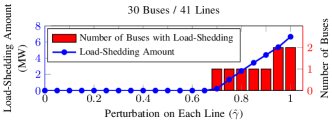
(a) Even distribution of relative impedance changes

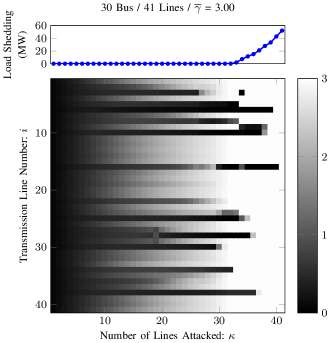
(b) “Safe” distribution of relative impedance changes, to minimize total power adjustment

Figure 1: Power adjustment as a result of changes to line impedances on the 30-Bus data set. It is often the case that load shedding is not required even when the disturbance to the system is quite substantial.

As mentioned above, the objective value of the bilevel formulation is zero for most feasible values of $\displaystyle\gamma$. It tends to be nonzero only on parts of the feasible region defined by (11b), (11c) that correspond to near-maximal attacks focused on small numbers of buses.

To illustrate this point, we perform experiments on the 30-Bus case (case30.m from MatPower, originally from [16]) in which we monitor the power-adjustment objective $\displaystyle{\cal F}_{L}(\gamma)$ in (7) as the impedances are increased. In Figure LABEL:sub@fig:30.perturb.evenly, we plot $\displaystyle{\cal F}_{L}(\gamma)$ in for the values $\displaystyle\gamma=\hat{\gamma}e$, where $\displaystyle\hat{\gamma}$ is a nonnegative scalar parameter that is increased progressively from $\displaystyle 0$ to $\displaystyle 1$. That is, impedances are increase evenly across all transmission lines. Note that $\displaystyle{\cal F}_{L}(\hat{\gamma}e)$ is zero for $\displaystyle\hat{\gamma}\in[0,0.65]$, while for $\displaystyle\hat{\gamma}>0.65$, load shedding occurs on one or two demand buses. This observation implies that any value $\displaystyle\gamma$ along the line $\displaystyle\hat{\gamma}e$ (for $\displaystyle\hat{\gamma}\in[0,.65]$) is a global minimizer of the bilevel problem (9). The gradient is zero at each of these points, so optimization methods that construct the search direction from gradients cannot make progress if started anywhere along this line (or indeed from anywhere in a large neighborhood of this line).

If we are allowed to distribute a “budget” of impedance increases unequally between lines, so as to minimize the total amount of power adjustment required, even greater disturbances can be tolerated. To describe this greater tolerance, we consider the following problem that is sliglty modified from (10):

$$\displaystyle{\cal H}_{S}(\kappa,\overline{\gamma}):=\min_{x,y,\gamma}\quad \displaystyle p^{T}y$$ (15a)

$$\displaystyle\operatorname*{subject\ to}.t.\quad \displaystyle F_{L}(x,y;\gamma)=0$$ (15b)

$$\displaystyle\underline{x}\leq x\leq\overline{x}$$ (15c)

$$\displaystyle 0\leq y\leq\overline{y}$$ (15d)

$$\displaystyle e^{T}\gamma=\kappa\overline{\gamma}$$ (15e)

$$\displaystyle 0\leq\gamma\leq\overline{\gamma}e.$$ (15f)

Note that (15) is different from (9) in two respects: (a) it is a single-level minimization problem whose variables are $\displaystyle x,y,$ and $\displaystyle\gamma$; and (b) the budget is enforced with the equality constraint (15e). Thus this problem finds a “safe” way to distribute the fixed budget ($\displaystyle\kappa\overline{\gamma}$) to transmission lines while the total load-shedding $\displaystyle p^{T}y$ is minimized. We solved this problem for an upper bound $\displaystyle\overline{\gamma}=3$ with $\displaystyle\kappa$, which is increased progressively from $\displaystyle 1$ to $\displaystyle 41$. The top chart in Figure LABEL:sub@fig:30.perturb.safely shows that it is possible to increase $\displaystyle\kappa$ to about $\displaystyle 33$ before any load shedding takes place at all. The lower chart depicts how the impedance changes are distributed around the 41 lines in the grid, at the solution of (15), for each value of $\displaystyle\kappa$. Darker bars on the graph show lines that can tolerate only a relatively small increase in impedance before causing load shedding somewhere in the grid. The lighter bars are those that can tolerate their impedance value $\displaystyle\gamma_{i}$ being set to a value at or near the upper bound $\displaystyle 3$ without affecting load shedding. As an example: When $\displaystyle\kappa=40$, we have $\displaystyle{\cal H}_{S}(40,3)\approx 55$, and the $\displaystyle\gamma$ that achieves this power-adjustment value has components of $\displaystyle 3$ on all lines except line $\displaystyle 16$, where it is zero.

The methodology used to derive Figure LABEL:sub@fig:30.perturb.safely can be used as a heuristic to identify a set of “safe” lines $\displaystyle{\cal S}$ (whose impedances can be increased without affecting grid performance) and a complementary set of “vulnerable” lines $\displaystyle{\cal W}$ (for which impedance increases are likely to lead to load shedding). In Appendix -B, we describe the ESL (“estimating safe lines”) procedure, Algorithm 3, for determining the sets $\displaystyle{\cal S}$ and $\displaystyle{\cal W}$. Once we have determined the vulnerable lines $\displaystyle{\cal W}$, we define an impedance perturbation vector $\displaystyle\gamma^{\prime}$ with the following components:

$$\gamma^{\prime}_{i}=\begin{cases}\overline{\gamma}&\;\;i\in{\cal W}\\ 0&\;\;i\notin{\cal W},\end{cases}$$ (16)

where $\displaystyle\overline{\gamma}$ is the given upper bound on impedance on a given line. We then evaluate $\displaystyle{\cal F}_{L}(\gamma^{\prime})$ from (7). If a node does not require any load shedding under this maximal-perturbation setting, it is unlikely that any attack on the vulnerable lines will lead to load shedding on this node. We gather the other nodes — those for which $\displaystyle\rho_{i}>0$ at the solution of (7h) with $\displaystyle\gamma=\gamma^{\prime}$ — into a set $\displaystyle{\cal T}$, the “target nodes.” Further explanation of the definition of $\displaystyle{\cal T}$ is given in Appendix -B2.

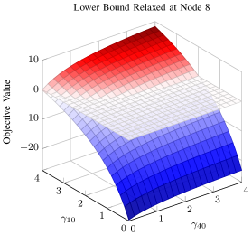
(a) Target node

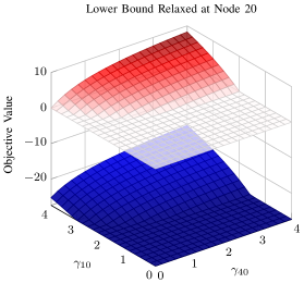
(b) Non-target node

Figure 2: Extending the range of $\displaystyle{\cal F}_{L}(\gamma)$ by allowing additional load on demand nodes. Adding load to target nodes (top figure) produces a useful extension of the range of the objective, so that its gradient yields a promising search direction for the maximization problem. Adding load to non-target nodes (bottom figure) simply shifts the objective down by a constant, so that the gradient in the flat region still does not yield a useful search direction for the maximization problem.

We use the target nodes to define a modification of the objective $\displaystyle{\cal F}_{L}$ that has the effect of shifting the range of the function, in a way that makes gradient information relevant even at values of $\displaystyle\gamma$ for which no power adjustments are required. The idea is illustrated in Figure 2, where we show the power-adjustment requirement on two different nodes (nodes 8 and 20) of the 30-Bus system as a function of the values of two impedance parameters — those corresponding to lines 10 and 40. In both graphs of Figure 2, the top surfaces (shaded white and red) represent the objective $\displaystyle{\cal F}_{L}$ as a function of various values of the pair $\displaystyle(\gamma_{10},\gamma_{40})$. Note that $\displaystyle{\cal F}_{L}$ takes the value zero over much of the domain, but becomes positive when both $\displaystyle\gamma_{10}$ and $\displaystyle\gamma_{40}$ are high. The lower surfaces in each graph show how $\displaystyle{\cal F}_{L}$ changes when we modify the subproblem in (7) by removing the zero lower lower bound on the load $\displaystyle\rho_{i}$ in (7h), where $\displaystyle i=8$ (a target node) in Figure LABEL:sub@fig:target.30.T and $\displaystyle i=20$ (a non-target node) in Figure LABEL:sub@fig:target.30.NT. Removal of the lower bound has the effect of allowing load to be added to the node in question. This is not an action that would be operationally desirable, but as we see from the blue surface in Figure LABEL:sub@fig:target.30.T, it changes the nature of $\displaystyle{\cal F}_{L}$ in useful ways. The effect of removing the lower bound on $\displaystyle\rho_{8}$ (Figure LABEL:sub@fig:target.30.T) is to extend the range of $\displaystyle{\cal F}_{L}$ so that its derivative at any point in the domain gives useful information about a good search direction. In a sense, the extended-range version appears to be a natural extension of the original objective $\displaystyle{\cal F}_{L}$. By contrast, removal of the lower bound on $\displaystyle\rho_{20}$ (Figure LABEL:sub@fig:target.30.NT) causes the function to simply be shifted downward by a roughly constant amount for all pairs of impedance perturbation values. This is because, being a non-target node, increased load on this node can be met, even after the grid is damaged by the impedance attack. We conclude that removing lower bounds on $\displaystyle\rho_{i}$ for target nodes $\displaystyle i\in{\cal T}$ provides a potentially useful extension of the range of the function $\displaystyle{\cal F}_{L}$, whereas the same cannot be said for non-target nodes.

Motivated by these observations, we modify Algorithm 1 as follows. We start by removing all lower bounds in (7h) on target nodes $\displaystyle i\in{\cal T}$. At each iteration of the algorithm, after taking a step, we check to see if any of the $\displaystyle\rho_{i}$ obtained by solving the subproblem (7) at the latest iteration are negative. If so, we reset the lower bound on the most negative value of $\displaystyle\rho_{i}$ to zero, before moving on to the next iteration. The algorithm does not terminate until all $\displaystyle\rho_{i}$ are nonnegative. The modified procedure is shown as Algorithm 2.

Algorithm 2 Vulnerability Analysis: Power-Adjustment Model

1:

2:$\displaystyle\overline{\gamma}$: Upper bound for impedance increases $\displaystyle\gamma_{i}$, $\displaystyle i\in{\cal L}$;

3:$\displaystyle\kappa$: Number of lines to attack;

4:$\displaystyle\gamma^{0}$: Feasible initial value of $\displaystyle\gamma$;

5:

6:$\displaystyle\gamma^{*}$: Impedance vector that optimizes the attack;

7:Find a set of vulnerable lines $\displaystyle{\cal W}$ and target nodes $\displaystyle{\cal T}$ using the ESL procedure (Algorithm 3);

8:Set lower bound of $\displaystyle\rho_{i}$ (for target nodes $\displaystyle i\in{\cal T}$) to $\displaystyle-\infty$;

9:$\displaystyle k\leftarrow 0$;

10:while $\displaystyle k\leq$MaxIter do

11:    Find gradient $\displaystyle g^{k}$ of $\displaystyle{\cal F}_{L}$ at $\displaystyle\gamma^{k}$.

12:    Find linearized optimum $\displaystyle w^{k}$ from (13);

13:    Use the backtracking to find step size $\displaystyle\alpha_{k}\in[0,1]$;

14:    $\displaystyle\gamma^{k+1}\leftarrow\gamma^{k}+\alpha_{k}(w^{k}-\gamma^{k})$;

15:    Identify $\displaystyle i$ such that $\displaystyle\rho_{i}=\arg\min_{j}\rho_{j}$, where $\displaystyle\rho_{j}$ are the

16:       power-adjustment variables from (7);

17:    if $\displaystyle\rho_{i}<0$ then

18:        reset lower bound on $\displaystyle\rho_{i}$ to zero;

19:    end if

20:    $\displaystyle k\leftarrow k+1$;

21:    Stop if terminating conditions (including $\displaystyle\rho_{j}\geq 0$ for all power-adjustment variables $\displaystyle\rho_{j}$) are satisfied;

22:end while

23:$\displaystyle\gamma^{*}\leftarrow\gamma^{k}$;

IV Experimental Results

We present the results obtained with our formulations and algorithms on the IEEE 118-Bus system and Polish 2383-Bus system. Our implementations use Matlab with Ipopt (Wächter and Biegler [17]) as the nonlinear solver for evaluating $\displaystyle{\cal F}_{L}$ (7) in the power-adjustment (bilevel) model. For the test case data and calculation of the electric circuit parameters, the codes from MatPower [18] are used extensively. The codes were executed on a Macbook Pro (2 GHz Intel Core i7 processor) with 8GB RAM.

TABLE I: Test Cases for Experiments

	Test Cases
	1	2	3	4
Filename (in MatPower)	case118.m		case2383wp.m
Number of Nodes	118		2383
Number of Lines	186		2896
Number of Lines to Attack $\displaystyle\kappa$	3	5	3	5
Perturbation Upper Bound $\displaystyle\overline{\gamma}$	3		2
Backtracking Parameters $\displaystyle(c_{0},c_{1},\alpha_{\min})$	(0.5, 0.01, 0.01)
Voltage limits $\displaystyle(\underline{V},\overline{V})$	$\displaystyle(0.93,1.07)$		$\displaystyle(0.89,1.12)$
Line Screening Threshold $\displaystyle\eta$	0.9

Information about the test case instances and algorithmic parameters are given in Table I. There are two instances for each of the two grids, corresponding to 3-line and 5-line attacks, respectively. The table shows voltage magnitude limits that are applied in the power-adjustment model, together with the value of $\displaystyle\eta$ that is used in the ESL procedure (Algorithm 3 from Appendix -B1).

In the power-adjustment model (7), the upper bounds $\displaystyle\overline{\sigma}_{i}^{+}$, $\displaystyle\overline{\sigma}_{i}^{-}$, and $\displaystyle\overline{\rho}_{i}$ on the power-adjustment variables are set to 1 for most buses, thus allowing full load shedding. If a bus violates our assumption on power injection — that is, if $\displaystyle P_{i}\leq 0$ for bus $\displaystyle i\in{\cal G}$ or $\displaystyle P_{i}\geq 0$ or $\displaystyle Q_{i}\geq 0$ for bus $\displaystyle i\in{\cal D}$ — the load-shedding upper bound for that bus is set to 0, disallowing power adjustment on that bus. The power-adjustment objective $\displaystyle{\cal F}_{L}$ is considered to be nonzero if it is at least $\displaystyle 10^{-3}$ megawatt (MW).

IV-A Voltage Disturbance Model

We discuss first results obtained with the voltage disturbance model (4)-(5) applied to the four test cases of Table I.

118-Bus System

For a 3-line attack problem on IEEE 118-Bus system ($\displaystyle\kappa=3$), Algorithm 1 converges in 5 iterations and identifies exactly three lines to attack with maximal impedance increase: lines 71, 74, and 82 (as shown in Table II). As a result of this attack, voltage magnitudes at four buses decrease significantly, by up to 0.07 p.u., as shown in Figure 3. (In Figure LABEL:sub@fig:result.volt.118.k3.mag, the buses are reordered in increasing order of voltage magnitude on the undisturbed system. In Figure LABEL:sub@fig:result.volt.118.k3.change, the buses are indexed in their original order.) The attack is visualized in Figure 5, where we see that its effect is essentially to isolate buses 51, 52, 53, and 58; the attacked lines are colored in red.

TABLE II: Voltage Disturbance Model: 118-Bus System with $\displaystyle\kappa=3$

Line Buses Continuous No. From To Attack ($\displaystyle\gamma_{i}$) 71 49 51 3.00 74 53 54 3.00 82 56 58 3.00 Objective $\displaystyle 4.04\times 10^{-2}$

(a) Optimal Attack (as determined by our algorithm)

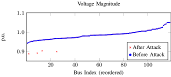
(a) Distribution of Voltage Magnitudes Before and After Attack.

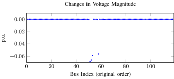
(b) Distribution of Voltage Magnitudes Changes After Attack.

Figure 3: Voltage Disturbance Model: 118-Bus System with $\displaystyle\kappa=3$

TABLE III: Voltage Disturbance Model: 118-Bus System with $\displaystyle\kappa=5$

Line Buses Continuous No. From To Attack ($\displaystyle\gamma_{i}$) 25 19 20 3.00 29 22 23 3.00 71 49 51 3.00 74 53 54 3.00 82 56 58 3.00 Objective $\displaystyle 5.03\times 10^{-2}$

(a) Optimal Attack (as determined by our Algorithm)

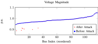
(a) Distribution of Voltage Magnitude Before and After Attack.

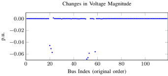
(b) Distribution of Voltage Magnitude Changes and After Attack.

Figure 4: Voltage Disturbance Model: 118-Bus System with $\displaystyle\kappa=5$

For the second test instance, on the IEEE 118-Bus system with $\displaystyle\kappa=5$, the algorithm identifies exactly five lines to attack at the maximal impedance increase — lines 25, 29, 71, 74, and 82 (see Table III) — which includes the three lines identified in the first attack. With this stronger attack, there is significant voltage drop on seven buses. Algorithm 1 takes 8 iterations to converge to the solution. As Figure 5 shows, attacking the additional two lines (colored in green) has the effect of creating another “island,” consisting of buses 20, 21 and 22. The additional voltage drops seen Figure LABEL:sub@fig:result.volt.118.k5.change are from these buses.

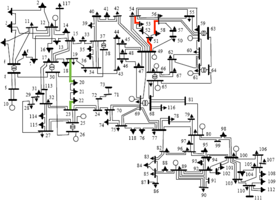
Figure 5: Voltage Disturbance Model: Attacks on the 118-Bus System. The transmission lines in red are are the optimal attack for $\displaystyle\kappa=3$. The lines in green are added to the optimal 3-line attack when $\displaystyle\kappa$ is increased to 5.

2383-Bus System

TABLE IV: Voltage Disturbance Model: 2383-Bus System with $\displaystyle\kappa=3$

Line	Buses		Continuous	Top-3	Best-3
No.	From	To	Attack ($\displaystyle\gamma_{i}$)	Attack	Attack
5	10	3	1.04	2.00	2.00
404	434	188	0.25
405	437	188	2.00	2.00	2.00
467	340	218	2.00	2.00	2.00
501	340	240	0.71
Objective			0.514	0.501	0.501

(a) Optimal Attack (as determined by our Algorithm)

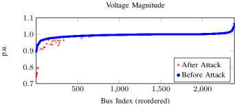
(a) Distribution of Voltage Magnitude Before and After Attack. (Best-3)

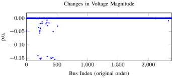
(b) Distribution of Voltage Magnitude Changes After Attack. (Best-3)

Figure 6: Voltage Disturbance Model: 2383-Bus System with $\displaystyle\kappa=3$

Results for our third test instance in Table I, which considers the 2383-Bus model with attack limit defined by $\displaystyle\kappa=3$, are shown in Table IV. The continuous impedance attack is distributed into 5 lines, identified after ten iterations of Algorithm 1. (The lines involved in the attack are revealed at iteration five, while the remaining five iterations make minor adjustments to the impedance values.)

This 5-line solution can be used to identify the most disruptive set of three lines using two heuristics: (a) choose the three lines $\displaystyle i$ such that $\displaystyle\gamma_{i}$ are one of the largest three entries in $\displaystyle\gamma$ (called the Top-3 attack); and (b) try all possible 3-line combinations of the five lines with highest impedance (the Best-3 attack). For this specific case, the Top-3 attack and Best-3 attack are the same, consisting of lines 5, 405, and 467. These 3-line attacks, with impedance set to their maximum values on all three lines, gives a slightly smaller objective value than the continuous attack.

Figure LABEL:sub@fig:result.volt.2383.k3.change shows how the voltage magnitude changes when the Best-3 and Top-3 attacks are executed. Similarly to 118-Bus cases, there is a relatively small number of buses in which the voltage drops significantly from its original value, but large voltage changes are seen on some buses, with some voltage magnitudes below 0.8 p.u.

For our fourth test instance in Table I, for which $\displaystyle\kappa=5$ on the 2383-Bus system, two iterations of Algorithm 1 suffice to identify an attack (on lines 404, 405, 467, 479, and 501) that makes the power flow problem infeasible, that is, there is no $\displaystyle(V,\theta)$ that satisfies $\displaystyle F(V,\theta;\gamma)=0$ under this attack. Hence, unless the grid operator takes action (to change loads or generator outputs, for example), an attack on these five lines renders the grid inoperable.

Comparison with Continuous Optimization Model

In Section II-B, we mentioned that the voltage disturbance model can be written as a continuous optimization model (6), except that the latter model does not handle infeasibility appropriately. We verify the properties of this alternative formulation by solving it with the nonlinear interior-point solver Ipopt. We find that in the first three instances of Table I, the solutions obtained from (5) match those we described above. In the fourth test case — the 2383-Bus model with $\displaystyle\kappa=5$ — the model (6) identifies a solution that maximizes disruption subject to the power flow equations (3) remaining feasible. Our model (5), which detects infeasibility of the grid under an attack of this strength, yields the more informative outcome.

IV-B Power-Adjustment Model

We now present results for the power-adjustment model (7), (9), for the four test instances of Table I.

118-Bus System

The ESL procedure (Algorithm 3), which is described in Section III-C and Appendix -B1, is applied to the 118-Bus system to identify vulnerable lines $\displaystyle{\cal W}=\{29,71,74,96,184\}$ and target nodes $\displaystyle{\cal T}=\{52,53,117\}$. We use these settings of $\displaystyle{\cal W}$ and $\displaystyle{\cal T}$ in Algorithm 2 to solve the first two instances in Table I.

For the first test case ($\displaystyle\kappa=3$), Algorithm 2 terminates after eight iterations, at the attack shown in Table V. Four lines are involved in this attack; we reduce to three-line attacks “Top-3” and “Best-3” as in Subsection IV-A. The Top-3 and Best-3 attacks coincide (and are the same as those obtained for the voltage disturbance model in Subsection IV-A) and have a slightly smaller objective value than the continuous attack. We note that in these 3-line attacks, the voltage magnitudes of buses 52 and 53 are at their lower bound $\displaystyle\underline{V}=.93$, and load shedding is required for buses 51 and 53, the total amount of load shedding being 22.13 MW.

TABLE V: Power-Adjustment Model: 118-Bus System with $\displaystyle\kappa=3$

Line	Buses		Continuous	Top-3	Best-3
No.	From	To	Attack ($\displaystyle\gamma_{i}$)	Attack	Attack
71	49	51	3.00	3.00	3.00
72	51	52	0.26
74	53	54	3.00	3.00	3.00
82	56	58	2.74	3.00	3.00
Objective (MW)			22.39	22.13	22.13
Buses with Load Shedding			51, 52, 53	51, 53	51, 53
Buses at Voltage Boundary			52	52, 53	52, 53

TABLE VI: Five Most Effective Attacks from Exhaustive Enumeration: 118-Bus System with $\displaystyle\kappa=3$

Lines Selected			Power Adjustment (MW)
71	74	82	22.13
71	72	74	19.07
71	74	83	17.21
71	74	184	15.61
71	74	97	13.27

In Table VI, we show the top five three-line attacks obtained by enumerating all $\displaystyle 266,916$ possible three-line attacks on this grid. The most disruptive attack is indeed the one found by our algorithm.

TABLE VII: Power-Adjustment Model: 118-Bus System with $\displaystyle\kappa=5$

Line	Buses		Continuous	Top-5	Best-5
No.	From	To	Attack ($\displaystyle\gamma_{i}$)	Attack	Attack
71	49	51	3.00	3.00	3.00
72	51	52	0.36		3.00
74	53	54	3.00	3.00	3.00
75	49	54	0.74
76	49	54	0.81	3.00
81	50	57	0.29
82	56	58	3.00	3.00	3.00
97	64	65	0.80
184	12	117	3.00	3.00	3.00
Objective (MW)			27.16	25.79	26.87
Buses with Power Adjustment			51, 52, 53, 117	51, 53, 117	52, 53, 117
Buses at Voltage Boundary			52, 117	52, 53, 117	52, 117

For the second test instance (with $\displaystyle\kappa=5$), Algorithm 1 requires twelve iterations to converge, and distributes the impedance increases around nine lines, with the maximum perturbation ($\displaystyle\gamma_{i}=3$) on four of them; see Table VII. The Top-5 and Best-5 attacks each involve the four lines with maximum impedance increases, but differ in their choice of additional line. Three buses require load shedding in the Best-5 attack, compared to two in the Best-3 attack.

Unlike the previous results for $\displaystyle\kappa=3$, which target the same lines as the voltage disturbance model, the Best-5 attack identified in the power-adjustment model is slightly different from the Best-5 attack for the voltage-disturbance model. The power-adjustment attack targets the region around buses 51, 52, and 53, as before, but also “islands” bus 117 (see Figure 5), rather than the buses 20, 21, and 22 that are attacked by the voltage-disturbance model.

2383-Bus System

For the Polish 2383-Bus system, the ESL procedure (Algorithm 3) identified a set $\displaystyle{\cal W}$ of 20 vulnerable lines and, for upper bound $\displaystyle\overline{\gamma}=2$ on the impedance increase, a set $\displaystyle{\cal T}$ of 55 target nodes. (Algorithm 3 required about 270 seconds of run time on this instance.)

TABLE VIII: Power-Adjustment Model: 2383-Bus System with $\displaystyle\kappa=3$

Line	Buses		From Bilevel Formulation			From $\displaystyle N-1$
No.	From	To	Cont. ($\displaystyle\gamma_{i}$)	Top-3	Best-3	Top-3	Best-3
5	10	3				2.00
264	140	117	0.02
268	126	118	2.00	2.00	2.00	2.00	2.00
289	135	125	1.98	2.00	2.00		2.00
296	145	128	2.00	2.00	2.00	2.00	2.00
Objective (MW)			577.80	577.75	577.75	303.07	577.75
# of Buses with Power Adjustment			49			27	49
Buses at Voltage Boundary			145, 146, 1905			145, 146, 230, 1905	145, 146, 1905

Results for the power-adjustment model on or our third test case from Table I, for the 2383-Bus system with $\displaystyle\kappa=3$, are shown in Table VIII. Algorithm 2 returns a four-line attack. Since the attack on one of these four lines (line 264) is negligible, we find that the Top-3 and Best-3 solutions both attack lines 268, 289 and 296, with an active-power load shedding 577.75 MW, which is negligibly smaller than the optimal four-line attack. There are 49 buses which need load shedding for the three-line attack, and three buses have voltage magnitudes at their lower limits of $\displaystyle\underline{V}=.89$ — another sign of stress on the grid. The solution obtained for this test case is quite different from the one from the voltage disturbance model. The lines 5, 404, 405, 467, and 501 which are identified by the voltage disturbance model (cf. Table IV) also cause some load shedding when they are attacked, but the effect is not as serious as the attack on lines 268, 289, and 296.

Since it is computationally intractable to look at all possible three-line combinations in a 2383-Bus grid, we apply an “$\displaystyle N-1$ enumeration” heuristic to explore the most promising part of the space of three-line attacks. In this heuristic, each line $\displaystyle i$ is individually perturbed by setting $\displaystyle\gamma_{i}=\overline{\gamma}$, and we note which of these perturbations require load shedding. On this data set, sixteen lines were identified as causing load shedding. We define a “Top-3$\displaystyle(N-1)$” attack to comprise the three lines that individually cause the most load shedding, and the “Best-3$\displaystyle(N-1)$” attack to be the most disruptive three-line combination drawn from these sixteen lines. The resulting attacks are displayed in Table VIII, alongside the Top-3 attack and Best-3 attack. We see that the Best-3$\displaystyle(N-1)$ attack is identical to the Top-3 and Best-3 attacks, while the Top-3$\displaystyle(N-1)$ attack is inferior.

The optimal attacks for the power-adjustment model in this third test instance are quite different from those obtained from the voltage disturbance model, as we see by comparing Tables IV and VIII. We found, however, that if the lower bound on voltage magnitude is changed from $\displaystyle\underline{V}=.89$ to $\displaystyle\underline{V}=.87$, the optimal attack for the power-adjustment model is almost identical to the voltage disturbance model. In the relaxed problem, the buses 145, 146, and 1905 no longer have their voltage magnitude at the lower bound, while buses 401 and 414 move to the relaxed lower bound. The latter two buses are among those that suffer significant voltage drop in the optimal voltage-disturbance attack of Table IV.

TABLE IX: Power-Adjustment Model: 2383-Bus System with $\displaystyle\kappa=5$

Line	Buses		From Bilevel Formulation			From $\displaystyle N-1$
No.	From	To	Cont. ($\displaystyle\gamma_{i}$)	Top-5	Best-5	Top-5	Best-5
5	10	3				2.00
268	126	118	2.00	2.00	2.00	2.00	2.00
269	142	118	2.00	2.00	2.00
289	135	125	2.00	2.00	2.00	2.00	2.00
296	145	128	2.00	2.00		2.00	2.00
317	142	135	1.54	2.00	2.00
405	437	188				2.00	2.00
467	340	218					2.00
2142	1693	1658	0.46		2.00
Objective (MW)			1109.72	1086.67	1460.25	594.09	597.71
# of Buses with Power Adjustment			77	78	71	53	53
Buses at Voltage Boundary			145, 146, 1905		1905	145, 146, 230, 414, 434, 1905	145, 146, 401, 414, 1905

Table IX shows results for our fourth test instance from Table I, an optimal attack on the 2383-Bus system for $\displaystyle\kappa=5$. The attack determined by our procedure is distributed around 6 lines. The Top-5, Best-5, Top-5$\displaystyle(N-1)$, and Best-5$\displaystyle(N-1)$ attacks are calculated as described above. The Best-5 attack is significantly more disruptive than the optimal continuous attack identified by Algorithm 2, probably because of nonconcavity in the objective $\displaystyle{\cal F}_{L}$. We note however that our algorithm is much more useful in screening for the most disruptive collection of lines than is the standard “$\displaystyle N-1$” screening methodology: The Top-5 and Best-5 attacks are much more damaging than the Top-5$\displaystyle(N-1)$ and Best-5$\displaystyle(N-1)$ attacks.

V Conclusions

We have proposed an attack model for assessing the vulnerability of power grids. The attack consists in increasing the impedance of transmission lines, with the resulting disruption to the grid measured in two ways. The first technique is to observe changes in voltage magnitudes at the buses; greater changes from the nominal values indicate greater disruption. The second technique is to measure the weighted sum of adjustments to load and generation that are needed to restore stable operation of the grid, with the voltage magnitudes confined to certain prespecified ranges. The two criteria give rise to optimization problems with different properties. Both are solved with a combination of known algorithms (such as Frank-Wolfe) and heuristics that determine promising regions of the solution space.

In our computational results, we also use our algorithm as a screening procedure for determining which collections of lines are likely to cause the most disruptive attacks. By enumerating combinations of lines from among those identified by our algorithms, we identify more disruptive attacks than those produced by alternative screening methods, such as the well known “$\displaystyle N-1$” criterion.

-A Computing Gradients

We describe here calculation of gradients for the functions $\displaystyle{\cal F}(\gamma)$ defined in Section II, which quantify the grid disruption arising from an attack modeled by the impedance vector $\displaystyle\gamma$. Both model functions considered here — (4) and (7) — have the following form:

$$\displaystyle{\cal F}(\gamma):=\min_{z}\quad \displaystyle f(z)$$ (17a)

$$\displaystyle\operatorname*{subject\ to}.t.\quad \displaystyle c_{i}(z,\gamma)=0,\quad i=1,2,\dotsc,m,$$ (17b)

$$\displaystyle h_{j}(z)\geq 0,\quad j=1,2,\dotsc,r,$$ (17c)

where the functions $\displaystyle f$, $\displaystyle c_{i}$, $\displaystyle i=1,2,\dotsc,m$, and $\displaystyle h_{j}$, $\displaystyle j=1,2,\dotsc,r$ are all smooth. (Note that in our models, the dependence on the upper-level variables $\displaystyle\gamma$ arises only through the equality constraints, but our discussion can be extended without conceptual difficulty to the case in which the objective and the inequality constraints also depend on $\displaystyle\gamma$.)

We outline a technique for calculating the gradient $\displaystyle\nabla{\cal F}(\gamma)$. We assume that the minimizing $\displaystyle z$ for the (generally nonconvex) problem (17) has been identified and that it is denoted by $\displaystyle z(\gamma)$. Moreover, we assume that $\displaystyle z(\gamma)$ is a nondegenerate solution of the minimization problem in (17). By this we mean that the linear independence constraint qualification holds at the minimizer, that a strict complementarity condition holds, and that second-order sufficient conditions are satisfied at $\displaystyle z(\gamma)$. We show that under these conditions, we can use the implicit function theorem to define the gradient $\displaystyle\nabla{\cal F}(\gamma)$ uniquely. While strong, these conditions are not impractical; they appear to hold for all values of $\displaystyle z(\gamma)$ encountered by our algorithm, and it seems plausible that they would hold for “almost all” values of $\displaystyle\gamma$. The question of existence of $\displaystyle\nabla{\cal F}(\gamma)$ becomes much more complicated when these conditions are not satisfied. When strict complementarity does not hold, for example, the set of active inequality constraints is on the verge of changing, an event usually associated with a point of nonsmoothness of $\displaystyle{\cal F}(\gamma)$.

The Karush-Kuhn-Tucker (KKT) conditions for optimality of $\displaystyle z$ in the problem (17) for a given $\displaystyle\gamma$ are that there exist scalars $\displaystyle\lambda_{i}$, $\displaystyle i=1,2,\dotsc,m$ and $\displaystyle\mu_{j}$, $\displaystyle j=1,2,\dotsc,r$ such that

$$\displaystyle\nabla f(z)-\sum_{i=1}^{m}\lambda_{i}\nabla_{z}c_{i}(z,\gamma)-\sum_{j=1}^{r}\mu_{j}\nabla h_{j}(z)=0,$$ (18a)

$$\displaystyle c_{i}(z,\gamma)=0,\;\;i=1,2,\dotsc,m,$$ (18b)

$$\displaystyle\mu_{j}\geq 0,\;\;j\in{\cal A}(z),$$ (18c)

$$\displaystyle h_{j}(z)=0,\;\;j\in{\cal A}(z),$$ (18d)

$$\displaystyle\mu_{j}=0,\;\;j\in\{1,2,\dotsc,r\}\setminus{\cal A}(z),$$ (18e)

$$\displaystyle h_{j}(z)\geq 0,\;\;j\in\{1,2,\dotsc,r\}\setminus{\cal A}(z),$$ (18f)

where the active set $\displaystyle{\cal A}(z)$ is defined as follows:

$${\cal A}(z):=\{j=1,2,\dotsc,r\,:\,h_{j}(z)=0\}.$$ (19)

We use the following vector notation:

$$c(z,\gamma) =[c_{i}(z,\gamma)]_{i=1}^{m}, \quad\lambda =[\lambda_{i}]_{i=1}^{m},$$

$$\mu_{\cal A} =[\mu_{j}]_{j\in{\cal A}}, \quad h_{\cal A}(z) =[h_{j}(z)]_{j\in{\cal A}}.$$

The linear independence constraint qualification (LICQ) is:

$$\{\nabla_{z}c_{i}(z,\gamma),\;i=1,2,\dotsc,m\}\cup\{\nabla h_{j}(z),\;j\in{\cal A}(z)\}$$    is a linearly independent set. (20)

The strict complementarity condition is that

$$\mu_{j}>0,\;\;\mbox{for all $\displaystyle j\in{\cal A}(z)$}.$$ (21)

Finally, the second-order sufficient conditions are

$$d^{T}W(z,\lambda,\mu,\gamma)d>0\;\;\mbox{for all $\displaystyle d\in N(z)$ with $\displaystyle d\neq 0$},$$ (22)

where the subspace $\displaystyle N(z)$ is defined as follows:

$$N(z):=\left\{d\,:\parbox{247.16656pt}{\centering$\displaystyle\nabla_{z}c_{i}(z,\gamma)^{T}d=0,\;i=1,2,\dotsc,m$ \\ and \\ $\displaystyle\nabla h_{j}(z)^{T}d=0,\;\forall j\in{\cal A}(z)$\@add@centering}\right\},$$ (23)

and the matrix $\displaystyle W(z,\lambda,\mu,\gamma)$ is the Hessian of the Lagrangian function for the problem (17), that is,

$$W( z,\lambda,\mu,\gamma)\,:=$$ (24)

$$\nabla^{2}f(z)-\sum_{i=1}^{m}\lambda_{i}\nabla^{2}_{zz}c_{i}(z,\gamma)-\sum_{j\in{\cal A}(z)}\mu_{j}\nabla^{2}h_{j}(z).$$

In the neighborhood of a value of $\displaystyle\gamma$ at which all the conditions above are satisfied, we find that $\displaystyle(z,\lambda,\mu_{\cal A})$ is an implicit function of $\displaystyle\gamma$. We find expressions for the derivatives of $\displaystyle(z,\lambda,\mu_{\cal A})$ with respect to $\displaystyle\gamma$ by applying the implicit function theorem (see for example [19, Theorem A.2]) to the equality conditions in (18), which we can formulate as follows:

$$\displaystyle\nabla f(z)-\sum_{i=1}^{m}\lambda_{i}\nabla_{z}c_{i}(z,\gamma) \displaystyle-\sum_{j\in{\cal A}(z)}\mu_{j}\nabla h_{j}(z)=0,$$ (25a)

$$\displaystyle c_{i}(z,\gamma) \displaystyle=0,\;\;i=1,2,\dotsc,m,$$ (25b)

$$\displaystyle h_{j}(z) \displaystyle=0,\;\;j\in{\cal A}(z).$$ (25c)

Note that this system of equations is square, with $\displaystyle n+m+|{\cal A}|$ equations and unknowns. Moreover, standard analysis of optimality conditions shows that its square Jacobian matrix is nonsingular, under the LICQ (20) and second-order sufficient (22) conditions. The implicit function theorem now yields the following:

$$\left[\begin{matrix}\nabla z(\gamma)\\ \nabla\lambda(\gamma)\\ \nabla\mu_{{\cal A}}(\gamma)\end{matrix}\right]=H(z,\lambda,\mu,\gamma)^{-1}\left[\begin{matrix}\sum_{i=1}^{m}\lambda_{i}\nabla_{z\gamma}c_{i}(z,\gamma)\\ -\nabla_{\gamma}c(z,\gamma)^{T}\\ 0\end{matrix}\right],$$ (26)

where

$$H(z,\lambda,\mu,\gamma)=\left[\begin{matrix}W(z,\lambda,\mu,\gamma)&-\nabla_{z}c(z,\gamma)&-\nabla h_{{\cal A}}(z)\\ \nabla_{z}c(z,\gamma)^{T}&0&0\\ \nabla h_{{\cal A}}(z)^{T}&0&0\end{matrix}\right].$$

We can derive $\displaystyle\nabla{\cal F}(z)$ from $\displaystyle\nabla z(\gamma)$ through the definition (17), as follows:

$$\nabla{\cal F}(\gamma)=\nabla z(\gamma)^{T}\nabla f(z(\gamma)).$$ (27)

-B Heuristics for Initializing the Power Adjustment Model

-B1 Determining Safe and Vulnerable Lines

We have noted that a typical grid contains many “safe” lines, for which large changes to the impedance do not affect the ability of the grid to serve demands. We discuss here a filtering approach to identify the complementary set of “vulnerable” lines, for which impedance change causes significant disruption of the grid. (We assume that the number of vulnerable lines is relatively small; otherwise, the grid has a systemic vulnerability and would be hard to defend.)

A naive approach for identifying safe and vulnerable lines is enumeration. For each line $\displaystyle i$, we set $\displaystyle\gamma=\overline{\gamma}e_{i}$ (where $\displaystyle e_{i}$ is a vector of all zeros except for $\displaystyle 1$ in the $\displaystyle i$th entry) and evaluate $\displaystyle{\cal F}_{L}(\gamma)$ defined by (8). Vulnerable lines are taken to be those for which $\displaystyle{\cal F}_{L}(\gamma)>0$. This enumeration approach is not very effective, in part because of its cost (it requires solution of $\displaystyle|{\cal L}|$ different power flow problems) and because it cannot identify combinations of lines that are individually “safe” but which together create a vulnerability in the network. We therefore propose an alternative heuristic called ESL (for “eliminating safe lines”).

The motivation of the ESL heuristic is as follow. If a system operator, instead of an attacker, is asked to increase impedance on exactly $\displaystyle\kappa$ lines, then he will choose those $\displaystyle\kappa$ lines so as to minimize the disruption to the system. These lines will not be an attractive choice on the attacker’s side, especially when increase of impedances on these lines does not lead to any load shedding, so in general we declare these lines to be “safe.” On the other hand, the lines not selected by the operator correspond to those that may cause disruption and hence are an attractive target for attack. We declare such lines to be “vulnerable.”

In ESL, following the experiment graphed in Figure LABEL:sub@fig:30.perturb.safely, we seek the value of $\displaystyle\kappa$ in (9b) such that a total perturbation of size $\displaystyle\kappa\overline{\gamma}$ can be distributed to lines with little load shedding. Lines $\displaystyle i$ for which $\displaystyle\gamma_{i}\approx\overline{\gamma}$ are declared to be safe. This process is repeated until relatively few vulnerable lines remain. The appropriate value of $\displaystyle\kappa$ can be found by binary search, by solving the following modification of the problem in (15), which depends on a working set $\displaystyle{\cal W}\subset{\cal L}$ of lines not yet classified as safe:

$$\displaystyle{\cal H}_{\cal W}(\kappa,\overline{\gamma})=\min_{x,y,\gamma}\quad \displaystyle p^{T}y$$ (28a)

$$\displaystyle\operatorname*{subject\ to}.t.\quad \displaystyle F_{L}(x,y;\gamma)=0$$ (28b)

$$\displaystyle e^{T}\gamma=\kappa\overline{\gamma}$$ (28c)

$$\displaystyle\underline{x}\leq x\leq\overline{x}$$ (28d)

$$\displaystyle 0\leq y\leq\overline{y}$$ (28e)

$$\displaystyle 0\leq\gamma_{i}\leq\overline{\gamma} \displaystyle~{}~{}~{}i\in{\cal W}$$ (28f)

$$\displaystyle\gamma_{i}=0 \displaystyle~{}~{}~{}i\notin{\cal W}.$$ (28g)

Algorithm 3 Eliminating Safe Lines (ESL)

1:

2:$\displaystyle{\cal L}:$ Set of all lines;

3:$\displaystyle\eta\in(0,1)$: Threshold for screening;

4:

5:$\displaystyle{\cal W}$: a set of vulnerable lines;

6:$\displaystyle{\cal S}$: a set of safe lines;

7:$\displaystyle{\cal S}\leftarrow\emptyset$;

8:repeat

9:    $\displaystyle{\cal W}\leftarrow{\cal L}\backslash{\cal S}$;

10:    Define $\displaystyle\kappa^{*}$ to be the largest value of $\displaystyle\kappa$ for which $\displaystyle{\cal H}_{\cal W}(\kappa,\overline{\gamma})<\epsilon$;

11:    $\displaystyle{\cal S}^{\prime}\leftarrow\left\{i\,:\,{\gamma_{i}}/{\overline{\gamma}}\geq\eta,~{}i\in{\cal W}\right\}$; $\displaystyle\blacktriangleright$ newly determined “safe” lines

12:    $\displaystyle{\cal S}\leftarrow{\cal S}\cup{\cal S}^{\prime}$;

13:until $\displaystyle{\cal S}^{\prime}=\emptyset$

The complete procedure is shown in Algorithm 3. We start by putting all lines $\displaystyle{\cal L}$ into the working set $\displaystyle{\cal W}$, then successively eliminating from $\displaystyle{\cal W}$ those lines $\displaystyle i$ for which the solution of (28) yields $\displaystyle\gamma_{i}$ within a factor $\displaystyle\eta$ of the upper bound $\displaystyle\overline{\gamma}$. (We used $\displaystyle\eta=.9$.) The process is repeated until no new “safe” lines are identified. The lines remaining in $\displaystyle{\cal W}$ are then classified as “vulnerable.”

-B2 Target Node Selection

Our approach for selecting “target” nodes $\displaystyle{\cal T}$ in Algorithm 2 is based on maximum loadability. The maximum loadability problem is similar to feasibility restoration in that it seeks the boundary of the feasible region. However, rather than starting from an infeasible point (where the nominal loads cannot be served), it begins from a feasible grid and increases the loads until demands can no longer be met. The difference is illustrated in Figure 7, which shows the $\displaystyle PV$-curve for a particular demand node. When the grid is feasible with demand $\displaystyle P_{D}$, (right curve), the demand can be increased to $\displaystyle P_{D}^{\prime\prime}$ while retaining feasibility. The difference $\displaystyle P_{D}^{\prime\prime}-P_{D}$ can be regarded as the maximum loadability at this node. If the grid is infeasible (left curve) the demand must be reduced to $\displaystyle P_{D}^{\prime}$ before feasibility is recovered.

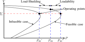
Figure 7: Loadability and Load Shedding in $\displaystyle PV$-curve

The formulation for maximum loadability problem can be obtained by replacing (7f), (7g), and (7h) by the following constraints:

$$\displaystyle\sigma_{i}^{+} \displaystyle=~{}0 \displaystyle~{}~{}~{}i\in{\cal G}$$ (29a)

$$\displaystyle\sigma_{i}^{-} \displaystyle=~{}0 \displaystyle~{}~{}~{}i\in{\cal G}$$ (29b)

$$\displaystyle\rho_{i} \displaystyle\leq~{}0 \displaystyle~{}~{}~{}i\in{\cal D}.$$ (29c)

The first two constraints fix the power generations at their nominal values, while (29c) allows increase (rather than decrease) of demand at the demand buses. When the nominal loads and generations are feasible, we expect the objective to be negative at the solution.

To identify the target nodes, we simply set $\displaystyle\gamma_{i}=\overline{\gamma}$ for all vulnerable lines $\displaystyle i\in{\cal W}$ that are identified by the ESL procedure, Algorithm 3, and solve (7) for this value of $\displaystyle\gamma$. If a node does not require any load shedding under this maximal-perturbation setting, it is unlikely that any attack on the vulnerable lines will lead to load shedding on this node. The target nodes are defined to be those for which load shedding is required, that is, $\displaystyle\rho_{i}>0$ at the solution of (7). We denote the set of these nodes by $\displaystyle{\cal T}$.

Figure 8 shows target and non-target nodes, and shows how maximum loadability motivates their classification into these categories. The top figure shows a non-target node, for which is it possible to meet the original demand $\displaystyle P_{D}$ even after the maximum-perturbation attack, though the loadability is decreased. The bottom figure shows that the demand must be reduced to $\displaystyle P_{D}^{\prime}$ in order for the network to remain feasible. On this node, there is a chance that an attack on the vulnerable lines will lead to load shedding. The target nodes are the nodes affected by the type of attack we are considering, so that even for a choice of $\displaystyle\gamma$ that allows the nominal demand on these loads to be served, the change in maximum loadability may give us some information on the sensitivity of demand that can be served to the value of $\displaystyle\gamma$. Since the objective in (7) is of weighted $\displaystyle\ell_{1}$ type, we expect the number of target nodes to be small.

The target nodes $\displaystyle{\cal T}$ are incorporated into Algorithm 2 by replacing the lower bound (7h) in the formulation (7) by a negative quantity for the nodes in $\displaystyle{\cal T}$, and increasing these bounds toward zero progressively during the course of Algorithm 2. Additional details are given in Subsection III-C.

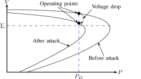
(a) Non-Target Node (No Load Shedding Required)

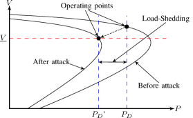
(b) Target Node (Load Shedding Required)

Figure 8: Possible Changes of $\displaystyle PV$-curve on a Node After Attack.

Taedong Kim received the B.S. degree in Computer Science and Engineering from Seoul National University, Seoul, South Korea in 2007, and M.S. degree in Computer Sciences from the University of Wisconsin-Madison (UW-Madison) in 2010. He is currently pursuing the Ph.D degree in Computer Sciences at UW-Madison. His research interests lie on applications of numerical optimization techniques to problems in sciences and engineering.

Stephen J. Wright received the B.Sc. (Hons.) and Ph.D. degrees from the University of Queensland, Australia, in 1981 and 1984, respectively. After holding positions at North Carolina State University, Argonne National Laboratory, and the University of Chicago, he joined the Computer Sciences Department at the University of Wisconsin-Madison as a Professor in 2001. His research interests include theory, algorithms, and applications of computational optimization. Dr. Wright was Chair of the Mathematical Programming Society from 2007-2010 and served from 2005-2014 on the Board of Trustees of the Society for Industrial and Applied Mathematics (SIAM). He has served on the editorial boards of Mathematical Programming (Series A), SIAM Review, and the SIAM Journal on Scientific Computing. He has been editor-in-chief of Mathematical Programming (Series B) and is current editor-in-chief of the SIAM Journal on Optimization.

Daniel Bienstock is a professor at the Departments of Industrial Engineering and Operations Research and Department of Applied Physics and Applied Mathematics, Columbia University, where he has been since 1989. His research focuses on optimization and computing, with special interest in power grid modeling and analysis.

Sean Harnett is a PhD student at the Department of Applied Physics and Applied Mathematics, Columbia University.

References

- [1] J. Salmeron, K. Wood, and R. Baldick, “Analysis of electric grid security under terrorist threat,” IEEE Transactions on Power Systems, vol. 19, no. 2, pp. 905–912, May 2004.
- [2] A. L. Motto, J. M. Arroyo, and F. D. Galiana, “A Mixed-Integer LP procedure for the analysis of electric grid security under disruptive threat,” IEEE Transactions on Power Systems, vol. 20, no. 3, pp. 1357–1365, Aug. 2005.
- [3] J. M. Arroyo and F. D. Galiana, “On the solution of the bilevel programming formulation of the terrorist threat problem,” IEEE Transactions on Power Systems, vol. 20, no. 2, pp. 789–797, May 2005.
- [4] J. Salmeron, K. Wood, and R. Baldick, “Worst-case interdiction analysis of large-scale electric power grids,” IEEE Transactions on Power Systems, vol. 24, no. 1, pp. 96–104, Feb. 2009.
- [5] V. Donde, V. López, and B. C. Lesieutre, “Severe multiple contingency screening in electric power systems,” IEEE Transactions on Power Systems, vol. 23, no. 2, pp. 406–417, May 2008.
- [6] A. Pinar, J. Meza, V. Donde, and B. C. Lesieutre, “Optimization strategies for the vulnerability analysis of the electric power grid,” SIAM Journal on Optimization, vol. 20, no. 4, pp. 1786–1810, 2010.
- [7] J. Arroyo, “Bilevel programming applied to power system vulnerability analysis under multiple contingencies,” IET Generation, Transmission & Distribution, vol. 4, no. 2, pp. 178–190, Sep. 2010.
- [8] A. Delgadillo, J. M. Arroyo, and N. Alguacil, “Analysis of electric grid interdiction with line switching,” IEEE Transactions on Power Systems, vol. 25, no. 2, pp. 633–641, May 2010.
- [9] J. M. Arroyo and F. J. Fernández, “Application of a genetic algorithm to power system security assessment,” International Journal of Electrical Power & Energy Systems, vol. 49, pp. 114–121, Jul. 2013.
- [10] D. Bienstock and A. Verma, “The problem in power grids: new models, formulations, and numerical experiments,” SIAM Journal on Optimization, vol. 20, no. 5, pp. 2352–2380, 2010.
- [11] U.S.-Canada Power System Outage Task Force, “Report on the august 14, 2003 blackout in the united states and canada: Causes and recommendations,” 2004. [Online]. Available: https://reports.energy.gov
- [12] A. R. Bergen and V. Vittal, Power systems analysis, 2nd ed. Prentice Hall, Aug. 1999.
- [13] K. Iba, S. Iwamoto, and Y. Tamura, “A method of finding multiple load-flow solutions for actual power systems,” Electrical Engineering in Japan, vol. 100, no. 3, pp. 257–264, May 1980.
- [14] M. Frank and P. Wolfe, “An algorithm for quadratic programming,” Naval research logistics quarterly, vol. 3, no. 1-2, pp. 95–110, Mar. 1956.
- [15] J. C. Dunn, “Convergence rates for conditional gradient sequences generated by implicit step length rules,” SIAM Journal on Control and Optimization, vol. 18, no. 5, pp. 473–487, 1980.
- [16] O. Alsac and B. Stott, “Optimal load flow with steady-state security,” IEEE Transactions on Power Apparatus and Systems, vol. PAS-93, no. 3, pp. 745–751, May 1974.
- [17] A. Wächter and L. Biegler, “On the implementation of an interior-point filter line-search algorithm for large-scale nonlinear programming,” Mathematical Programming, vol. 106, no. 1, pp. 25–57, Mar. 2006.
- [18] R. D. Zimmerman, C. E. Murillo-Sánchez, and R. J. Thomas, “MATPOWER: Steady-state operations, planning, and analysis tools for power systems research and education,” IEEE Transactions on Power Systems, vol. 26, no. 1, pp. 12–19, Feb. 2011.
- [19] J. Nocedal and S. J. Wright, Numerical Optimization, 2nd ed. New York: Springer, 2006.