Robust Anomaly Detection in Dynamic Networks 1

Abstract

We propose two robust methods for anomaly detection in dynamic networks in which the properties of normal traffic are time-varying. We formulate the robust anomaly detection problem as a binary composite hypothesis testing problem and propose two methods: a model-free and a model-based one, leveraging techniques from the theory of large deviations. Both methods require a family of Probability Laws (PLs) that represent normal properties of traffic. We devise a two-step procedure to estimate this family of PLs. We compare the performance of our robust methods and their vanilla counterparts, which assume that normal traffic is stationary, on a network with a diurnal normal pattern and a common anomaly related to data exfiltration. Simulation results show that our robust methods perform better than their vanilla counterparts in dynamic networks.

I Introduction

A network anomaly is any potentially malicious traffic sequence that has implications for the security of the network. Although automated online traffic anomaly detection has received a lot of attention, this field is far from mature.

Network anomaly detection belongs to a broader field of system anomaly detection whose approaches can be roughly grouped into two classes: signature-based anomaly detection, where known patterns of past anomalies are used to identify ongoing anomalies [1, 2], and change-based anomaly detection that identifies patterns that substantially deviate from normal patterns of operations [3, 4, 5]. [6] showed that the detection rates of systems based on pattern matching are below 70%. Furthermore, such systems cannot detect zero-day attacks, i.e., attacks not previously seen, and need constant (and expensive) updating to keep up with new attack signatures. In contrast, change-based anomaly detection methods are considered to be more economic and promising since they can identify novel attacks. In this work we focus on change-based anomaly detection methods, in particular on statistical anomaly detection that leverages statistical methods.

Standard statistical anomaly detection consists of two steps. The first step is to learn the “normal behavior” by analyzing past system behavior; usually a segment of records corresponding to normal system activity. The second step is to identify time instances where system behavior does not appear to be normal by monitoring the system continuously.

For anomaly detection in networks, [5] presents two methods to characterize normal behavior and to assess deviations from it based on the Large Deviations Theory (LDT) [7]. Both methods consider the traffic, which is a sequence of flows, as a sample path of an underlying stochastic process and compare current network traffic to some reference network traffic using LDT. One method, which is referred to as the model-free method, employs the method of types [7] to characterize the type (i.e., empirical measure) of an independent and identically distributed (i.i.d.) sequence of network flows. The other method, which is referred to as the model-based method, models traffic as a Markov Modulated Process. Both methods rely on a stationarity assumption postulating that the properties of normal traffic in networks do not change over time.

However, the stationarity assumption is rarely satisfied in contemporary networks [8]. For example, Internet traffic is subject to weekly and diurnal variations [9, 10]. Internet traffic is also influenced by macroscopic factors such as important holidays and events [11]. Similar phenomena arise in local area networks as well. We will call a network dynamic if its traffic exhibits time-varying behavior.

The challenges for anomaly detection of dynamic networks are two-fold. First, the methods used for learning the “normal behavior” are usually quite sensitive to the presence of non-stationarity. Second, the modeling and prediction of multi-dimensional and time-dependent behavior is hard.

To address these challenges, we generalize the vanilla model-free and model-based methods from [5] and develop what we call the robust model-free and the robust model-based methods. The novelties of our new methods are as follows. First, our methods are robust and optimal in the generalized Neyman-Pearson sense. Second, we propose a two-stage method to estimate Probability Laws (PLs) that characterize normal system behaviors. Our two-stage method transforms a hard problem (i.e., estimating PLs for multi-dimensional data) into two well-studied problems: $(i)$ estimating one-dimensional data parameters and $(ii)$ the set cover problem. Being concise and interpretable, our estimated PLs are helpful not only in anomaly detection but also in understanding normal system behavior.

The structure of the paper is as follows. Sec. II formulates system anomaly detection as a binary composite hypothesis testing problem and proposes two robust methods. Sec. III applies the methods presented in Sec. II. Sec. IV explains the simulation setup and presents results from our robust methods as well as their vanilla counterparts. Finally, Sec. V provides concluding remarks.

II Binary composite hypothesis testing

We model the network environment as a stochastic process and estimate its parameters through some reference traffic (viewed as sample paths). Then the problem of network anomaly detection is equivalent to testing whether a sequence of observations $\mathcal{G}=\{g^{1},\ldots,g^{n}\}$ is a sample path of a discrete-time stochastic process $\mathscr{G}=\{G^{1},\ldots,G^{n}\}$ (hypothesis $\mathcal{H}_{0}$). All random variables $G^{i}$ are discrete and their sample space is a finite alphabet $\Sigma=\{\sigma_{1},\sigma_{2},\dots,\sigma_{|\Sigma|}\}$, where $|\Sigma|$ denotes the cardinality of $\Sigma$. All observed symbols $g^{i}$ belong to $\Sigma$, too. This problem is a binary composite hypothesis testing problem. Because the joint distribution of all random variables $G^{i}$ in $\mathscr{G}$ becomes complex when $n$ is large, we propose two types of simplification.

II-A A model-free method

We propose a model-free method that assumes the random variables $G^{i}$ are i.i.d. Each $G^{i}$ takes the value $\sigma_{j}$ with probability $p_{\theta}^{F}(G^{i}=\sigma_{j})$, $j=1,\ldots,|\Sigma|$, which is parameterized by $\theta\in\Omega$. We refer to the vector $\mathbf{p}_{\theta}^{F}=(p_{\theta}^{F}(G^{i}=\sigma_{1}),\ldots,p_{\theta}^{F}(G^{i}=\sigma_{|\Sigma|}))$ as the model-free Probability Law (PL) associated with $\theta$. Then the family of model-free PLs $\mathscr{P}^{F}=\left\{\mathbf{p}_{\theta}^{F}:\theta\in\Omega\right\}$ characterizes the stochastic process $\mathscr{G}$.

To characterize the observation $\mathcal{G}$, let

$$\mathscr{E}_{F}^{\mathcal{G}}(\sigma_{j})=\frac{1}{n}\sum_{i=1}^{n}\mathbf{1}(g^{i}=\sigma_{j}),\qquad j=1,\ldots,|\Sigma|,$$ (1)

where $\mathbf{1}(\cdot)$ is an indicator function. Then, an estimate for the underlying model-free PL based on the observation $\mathcal{G}$ is $\boldsymbol{\mathcal{E}}_{F}^{\mathcal{G}}=\left\{\mathscr{E}_{F}^{\mathcal{G}}(\sigma_{j}):\ j=1,\dots,|\Sigma|\right\}$, which is called the model-free empirical measure of $\mathcal{G}$.

Suppose $\boldsymbol{\mu}=(\mu(\sigma_{1}),\ldots,\mu(\sigma_{|\Sigma|}))$ is a model-free PL and $\boldsymbol{\nu}=(\nu(\sigma_{1}),\ldots,\nu(\sigma_{|\Sigma|}))$ is a model-free empirical measure. To quantify the difference between $\boldsymbol{\mu}$ and $\boldsymbol{\nu}$, we define the model-free divergence between $\boldsymbol{\mu}$ and $\boldsymbol{\nu}$ as

$$D_{F}(\boldsymbol{\nu}\|\boldsymbol{\mu})\triangleq\sum_{j=1}^{|\Sigma|}\hat{\nu}(\sigma_{j})\log\frac{\hat{\nu}(\sigma_{j})}{\hat{\mu}(\sigma_{j})},$$ (2)

where $\hat{\nu}(\sigma_{j})=\max(\nu(\sigma_{j}),\varepsilon)$ and $\hat{\mu}(\sigma_{j})=\max(\nu(\sigma_{j}),\varepsilon),\forall j$ and $\varepsilon$ is a small positive constant introduced to avoid underflow and division by zero.

Definition 1

(Model-Free Generalized Hoeffding Test). The model-free generalized Hoeffding test [12] is to reject $\mathcal{H}_{0}$ if $\mathcal{G}$ is in

$$S_{F}^{*}=\{\mathcal{G}\mid\inf_{\theta\in\Omega}\,D_{F}(\boldsymbol{\mathcal{E}}_{F}^{\mathcal{G}}\|\mathbf{p}_{\theta}^{F})\geq\lambda\},$$

where $\lambda$ is a detection threshold and $\inf_{\theta\in\Omega}\,D_{F}(\boldsymbol{\mathcal{E}}_{F}^{\mathcal{G}}\|\mathbf{p}_{\theta}^{F})$ is referred to as the generalized model-free divergence between $\boldsymbol{\mathcal{E}}_{F}^{\mathcal{G}}$ and $\mathscr{P}^{F}=\left\{\mathbf{p}_{\theta}^{F}:\theta\in\Omega\right\}$.

A similar definition has been proposed for robust localization in sensor networks [13]. One can show that this generalized Hoeffding test is asymptotically (as $n\rightarrow\infty$) optimal in a generalized Neyman-Pearson sense; we omit the technical details in the interest of space.

II-B A model-based method

We now turn to the model-based method where the random process $\mathscr{G}=\{G^{1},\ldots,G^{n}\}$ is assumed to be a Markov chain. Under this assumption, the joint distribution of $\mathscr{G}$ becomes $p_{\theta}\left(\mathscr{G}=\mathcal{G}\right)=p_{\theta}^{B}\left(g^{1}\right)\prod_{i=1}^{n-1}p_{\theta}^{B}\left(g^{i+1}\mid g^{i}\right)$, where $p_{\theta}^{B}(\cdot)$ is the initial distribution and $p_{\theta}^{B}\left(\cdot\mid\cdot\right)$ is the transition probability; all parametrized by $\theta\in\Omega$.

Let $p_{\theta}^{B}\left(\sigma_{i},\sigma_{j}\right)$ be the probability of seeing two consecutive states $(\sigma_{i},\sigma_{j})$. We refer to the matrix $\mathbf{P}_{\theta}^{B}=\{p_{\theta}^{B}(\sigma_{i},\sigma_{j})\}_{i,j=1}^{|\Sigma|}$ as the model-based PL associated with $\theta\in\Omega$. Then, the family of model-based PLs $\mathscr{P}^{B}=\left\{\mathbf{P}_{\theta}^{B}:\theta\in\Omega\right\}$ characterizes the stochastic process $\mathscr{G}$.

To characterize the observation $\mathcal{G}$, let

$$\mathscr{E}_{B}^{\mathcal{G}}(\sigma_{i},\sigma_{j})=\frac{1}{n}\sum_{l=2}^{n}\mathbf{1}(g^{l-1}=\sigma_{i},g^{l}=\sigma_{j}),i,j=1,\ldots,|\Sigma|.$$ (3)

We define the model-based empirical measure of $\mathcal{G}$ as the matrix $\boldsymbol{\mathcal{E}}_{B}^{\mathcal{G}}=\{\mathscr{E}_{B}^{\mathcal{G}}(\sigma_{i},\sigma_{j})\}_{i,j=1}^{|\Sigma|}$. The transition probability from $\sigma_{i}$ to $\sigma_{j}$ is simply $\mathscr{E}_{B}^{\mathcal{G}}(\sigma_{j}|\sigma_{i})=\frac{\mathscr{E}_{B}^{\mathcal{G}}(\sigma_{i},\sigma_{j})}{\sum_{j=1}^{|\Sigma|}\mathscr{E}_{B}^{\mathcal{G}}(\sigma_{i},\sigma_{j})}$.

Suppose $\boldsymbol{\Pi}=\{\pi(\sigma_{i},\sigma_{j})\}_{i,j=1}^{|\Sigma|}$ is a model-based PL and $\mathbf{Q}=\{q(\sigma_{i},\sigma_{j})\}_{i,j=1}^{|\Sigma|}$ is a model-based empirical measure. Let $\hat{\pi}(\sigma_{j}|\sigma_{i})$ and $\hat{q}(\sigma_{j}|\sigma_{i})$ be the corresponding transition probabilities from $\sigma_{i}$ to $\sigma_{j}$. Then, the model-based divergence between ${\boldsymbol{\Pi}}$ and $\mathbf{Q}$ is

$$D_{B}(\mathbf{Q}\parallel\boldsymbol{\Pi})=\sum_{i=1}^{|\Sigma|}\sum_{j=1}^{|\Sigma|}\hat{q}(\sigma_{i},\sigma_{j})\log\frac{\hat{q}(\sigma_{j}|\sigma_{i})}{\hat{\pi}(\sigma_{j}|\sigma_{i})},$$ (4)

where $\hat{q}(\sigma_{i},\sigma_{j})=\max(q(\sigma_{i},\sigma_{j}),\varepsilon)$, $\hat{\pi}(\sigma_{i},\sigma_{j})=\max(\pi(\sigma_{i},\sigma_{j}),\varepsilon)$ for some small positive constant $\varepsilon$ introduced to avoid underflow and division by zero. Similar to the model-free case, we present the following definition:

Definition 2

(Model-Based Generalized Hoeffding Test). The model-based generalized Hoeffding test is to reject $\mathcal{H}_{0}$ when $\mathcal{G}$ is in

$$S_{B}^{*}=\{\mathcal{G}\mid\inf_{\theta\in\Omega}\,D_{B}(\boldsymbol{\mathcal{E}}_{B}^{\mathcal{G}}\|\mathbf{P}_{\theta}^{B})\geq\lambda\},$$

where $\lambda$ is a detection threshold and $\inf_{\theta\in\Omega}\,D_{B}(\boldsymbol{\mathcal{E}}_{B}^{\mathcal{G}}\|\mathbf{P}_{\theta}^{B})$ is referred to as the generalized model-based divergence between $\boldsymbol{\mathcal{E}}_{F}^{\mathcal{G}}$ and $\mathscr{P}^{B}=\left\{\mathbf{P}_{\theta}^{B}:\theta\in\Omega\right\}$.

In this case as well, asymptotic (generalized) Neyman-Pearson optimality can be established.

III Network anomaly detection

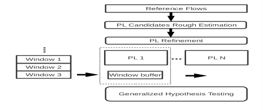
Fig. 1 outlines the structure of our robust anomaly detection methods. We first propose our feature set (Sec. III-A). We assume that the normal traffic is governed by an underlying stochastic process $\mathscr{G}$. We assume the size of model-free and model-based PL families to be finite and propose a two-step procedure to estimate PLs from some reference data. We first inspect each feature separately to generate a family of candidate PLs (Sec.III-C), which is then reduced to a smaller family of PLs (Sec. III-D). For each window, the algorithm applies the model-free and model-based generalized Hoeffding test discussed above.

Figure 1: Structure of the algorithms.

III-A Data representation

In this paper, we focus on host-based anomaly detection, a specific application in which we monitor the incoming and outgoing packets of a server. We assume that the server provides only one service (e.g., HTTP server) and other ports are either closed or outside our interests. As a result, we only monitor traffic on certain port (e.g., port 80 for HTTP service). For servers with multiple ports in need of monitoring, we can simply run our methods on each port.

The features we propose for this particular application relate to a flow representation slightly different from that of commercial vendors like Cisco NetFlow [14]. Hereafter, we will use “flows”, “traffic”, and “data” interchangeably. Let $\mathcal{S}=\{\mathbf{s}^{1},\dots,\mathbf{s}^{|\mathcal{S}|}\}$ denote the collection of all packets collected on certain port of the host which is monitored. In host-based anomaly detection, the server IP is always fixed, thus ignored. Denote the user IP address in packet ${\mathbf{s}}^{i}$ as ${\mathbf{x}}^{i}$, whose format will be discussed later. The size of ${\mathbf{s}}^{i}$ is $b^{i}\in[0,\infty)$ in bytes and the start time of transmission is $t^{i}\in[0,\infty)$ in seconds. Using this convention, packet ${\mathbf{s}}^{i}$ can be represented as $({\mathbf{x}}^{i},b^{i},t_{s}^{i})$ for all $i=1,\dots,|\mathcal{S}|$.

We compile a sequence of packets ${\mathbf{s}}^{1},\dots,{\mathbf{s}}^{m}$ with $t_{s}^{1}<\dots<t_{s}^{m}$ into a flow $\mathbf{f}=({\mathbf{x}},b,d_{t},t)$ if ${\mathbf{x}}={\mathbf{x}}^{1}=\dots={\mathbf{x}}^{m}$ and $t_{s}^{i}-t_{s}^{i-1}<\delta_{F}$ for $i=2,\dots,m$ and some prescribed $\delta_{F}\in(0,\infty)$. Here, the flow size $b$ is the sum of the sizes of the packets that comprise the flow. The flow duration is $d_{t}=t_{s}^{m}-t_{s}^{1}$. The flow transmission time $t$ equals the start time of the first packet of the flow $t_{s}^{1}$. In this way, we can translate the large collection of packets $\mathcal{S}$ into a relatively small collection of flows $\mathcal{F}$.

Suppose ${\mathcal{X}}$ is the set of unique IP addresses in ${\mathcal{F}}$. Viewing each IP as a tuple of integers, we apply typical $K$-means clustering on ${\mathcal{X}}$. For each ${\mathbf{x}}\in{\mathcal{X}}$, we thus obtain a cluster label $k({\mathbf{x}})$. Suppose the cluster center for cluster $k$ is $\bar{{\mathbf{x}}}^{k}$; then the distance of ${\mathbf{x}}$ to the corresponding cluster center is $d_{a}({\mathbf{x}})=d({\mathbf{x}},\bar{{\mathbf{x}}}^{k({\mathbf{x}})})$, for some appropriate distance metric. The cluster label $k(\mathbf{x})$ and distance to cluster center $d_{a}(\mathbf{x})$ are used to identify a user IP address $\mathbf{x}$, leading to our final representation of a flow as:

$$\mathbf{f}=(k({\mathbf{x}}),d_{a}({\mathbf{x}}),b,d_{t},t).$$ (5)

For each $\mathbf{f}$, we quantize $d_{a}(\mathbf{x})$, $b$, and $d_{t}$ to discrete values. Each tuple of $\left(k({\mathbf{x}}),d_{a}({\mathbf{x}}),b,d_{t}\right)$ corresponds to a symbol in $\Sigma=\{1,\dots,K\}\times\Sigma_{d_{a}}\times\Sigma_{b}\times\Sigma_{d_{t}}$, where $\Sigma_{d_{a}}$, $\Sigma_{b}$ and $\Sigma_{d_{t}}$ are the quantization alphabets for distance to cluster center, flow size, and flow duration, respectively. Denoting by $\mathbf{g}$ the corresponding quantized symbol of $\mathbf{f}$ and by $\mathcal{G}$ the counterpart of $\mathcal{F}$, we number the symbols in $\mathbf{g}$ corresponding to $k({\mathbf{x}})$, $d_{a}({\mathbf{x}})$, $b$, and $d_{t}$ as features 1, 2, 3, 4.

In our methods, flows in $\mathcal{F}$ are further aggregated into windows based on their flow transmission times. A window is a detection unit that consists of flows in a continuous time range, i.e., the flows in a same window are evaluated together. Let $h$ be the interval between the start points of two consecutive time windows and $w_{s}$ be the window size.

III-B Anomaly detection for dynamic networks

For each window $j$, an empirical measure of $\mathcal{G}_{j}$ is calculated. We then leverage the model-free and the model-based generalized Hoeffding test (Def. 1,2), which require a set of PLs $\{\mathbf{p}_{\theta}^{F}:\theta\in\Omega\}$ and $\{\mathbf{P}_{\boldsymbol{\theta}}^{B}:\theta\in\Omega\}$. We assume $|\Omega|$ to be finite, and divide our reference traffic $\mathcal{G}_{ref}$ into segments; the traffic of each segment is governed by the same PL. The empirical measure of each segment is then a PL.

Two flows are likely to be governed by a same PL if they have close flow transmission times. In addition, if the properties of the normal traffic change periodically, two flows are also likely be governed by a same PL when the difference of their flow transmission times is close to the period. Let $t_{p}$ be the period and let $t_{d}$ be a window size characterizing the speed of change for the normal pattern. We could divide each period into $\lfloor t_{p}/t_{d}\rfloor$ segments with length $t_{d}$, and combine corresponding segments of different periods together, resulting in $\lfloor t_{p}/t_{d}\rfloor$ PLs.

In practical networks, the period may vary with time, which makes it hard to estimate $t_{p}$ and $t_{d}$ accurately. To increase the robustness of the set of estimated PLs to these non-stationarities, we first propose a large collection of candidates (Sec. III-C) and then refine it (Sec. III-D).

III-C Estimation of $t_{d}$ and $t_{p}$

This section presents a procedure to estimate $t_{d}$ and $t_{p}$ by inspecting each feature separately. Recall that each quantized flow consists of quantized values of a cluster label, a distance to cluster center, a flow size and a flow duration, which are called features $1,\dots,4$, respectively. We say a quantized flow $\mathbf{g}$ belongs to channel $a\text{--}b$ if feature $a$ of $\mathbf{g}$ equals symbol $b$ in quantization alphabet of feature $a$. We first analyze each channel separately to get a rough estimate of $t_{d}$ and $t_{p}$. Then, channels corresponding to the same feature are averaged to generate a combined estimate.

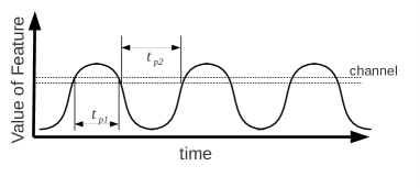
For all flows in channel $a\text{--}b$, we calculate the intervals between two consecutive flows. Most of the intervals will be very small. If we divide the interval length to several bins and calculate the histogram, i.e., the number of observed intervals in each bin. The histogram is heavily skewed to small interval length. $t_{d}$ could be chosen to be the interval length of the first bin (corresponding to the smallest interval length) whose frequency in the histogram is less than a threshold. In addition, there may be some large intervals if the feature is periodic. Fig. 2 shows an example of a feature that exhibits periodicity. There will be two peaks around $t_{p1}$ and $t_{p2}$ in the histogram of intervals for flows whose values are between the two dashed lines. We can select $t_{p}$ such that $\left(t_{p1}+t_{p2}\right)/2\thickapprox t_{p}/2$. There can be a single or more than two peaks due to noise in the network; in either case, we choose the average of all peaks as an estimate of $t_{p}/2$.

Figure 2: Illustration of the peaks in periodic networks.

If no channel of a feature $a$ reports $t_{p}$, the network is non-periodic according to the feature $a$. Otherwise, the estimate of $t_{p}$ for a feature $a$ (denoted by $t_{p}^{a}$) a is simply the average of all estimates for channels of the feature $a$. Although the estimate of only one channel is usually very inaccurate, the averaging procedure helps improve the accuracy. Similarly, the estimate for $t_{d}$ for a feature $a$ (denoted by $t_{d}^{a}$) is the average of the estimates for all channels of the feature $a$.

For each feature $a$, we generate some PLs using the estimate $t_{d}^{a}$ and $t_{p}^{a}$. In case that some prior knowledge of $t_{d}$ and $t_{p}$ is available, the family of candidate PLs can include the PLs calculated based on this prior knowledge.

III-D PL refinement with integer programming

The larger the family of PLs we use in generalized hypothesis testing, the more likely we will overfit $\mathcal{G}_{ref}$, leading to poor results. Furthermore, a smaller family of PLs reduces the computational cost. This section introduces a method to refine the family of candidate PLs.

For simplicity, we only describe the procedure for the model-free method. The procedure for the model-based method is similar. Hereafter, the divergence between a collection of flows and a PL is equivalent to the divergence between the empirical measure of these flows and the PL.

Suppose the family (namely the set) of candidate PLs is the set $\mathcal{P}=\{\mathbf{p}_{1}^{F},\dots,\mathbf{p}_{N}^{F}\}$ of cardinality $N$. Because no alarm should be reported for $\mathcal{G}_{ref}$, or any segment of $\mathcal{G}_{ref}$, our primary objective is to choose the smallest set $\mathscr{P}^{F}\subseteq\mathcal{P}$ such that there is no alarm for $\mathcal{G}_{ref}$. We aggregate $\mathcal{G}_{ref}$ into $M$ windows using the techniques of Sec. III-A and denote the data in window $i$ as $\mathcal{G}_{ref}^{i}$. Let $D_{ij}=D_{F}(\boldsymbol{\mathcal{E}}^{\mathcal{G}_{ref}^{i}}\parallel\mathbf{p}_{j}^{F})$ be the divergence between flows in window $i$ and PL $j$ for $i=1,\ldots,M$ and $j=1,\ldots,N$. We say window $i$ is covered (namely, reported as normal) by PL $j$ if $D_{ij}\leq\lambda$. With this definition, the primary objective becomes to select the minimum number of PLs to cover all the windows.

There may be more than one subsets of $\mathcal{P}$ having the same cardinality and covering all windows. We propose a secondary objective characterizing the variation of a set of PLs. Denote by $\mathscr{D}_{j}$ the set of intervals between consecutive window covered by PL $j$. The coefficient of variation for PL $j$ is defined as $c_{v}^{j}=\textsc{Std}(\mathscr{D}_{j})/\textsc{Mean}(\mathscr{D}_{j})$, where $\textsc{Std}(\mathscr{D}_{j})$ and $\textsc{Mean}(\mathscr{D}_{j})$ are the sample standard deviation and mean of set $\mathscr{D}{}_{j}$, respectively. A smaller coefficient of variation means that the PL is more “regular.”

We formulate PL refinement as a weighted set cover problem in which the weight of PL $j$ is $1+\gamma c_{v}^{j}$, where $\gamma$ is a small weight for the secondary objective. Let $x_{i}$ be the $0\text{--}1$ variable indicating whether PL $i$ is selected or not; let $\mathbf{x}=(x_{1},\ldots,x_{N})$. Let $\mathbf{A}=\{a_{ij}\}$ be an $M\times N$ matrix whose $(i,j)$th element $a_{ij}$ is set to $1$ if $D_{ij}\leq\lambda$ and to $0$ otherwise. Here, $\lambda$ is the same threshold we used in Def. 1. Let $\mathbf{c}_{v}=(c_{v}^{1},\ldots,c_{v}^{N})$. The selection of PLs can be formulated as the following integer programming problem:

$$\begin{array}[]{rl}\min&\mathbf{1}^{{}^{\prime}}\mathbf{x}+\gamma\mathbf{c}_{v}^{{}^{\prime}}\mathbf{x}\\ \text{s.t.}&\mathbf{A}\mathbf{x}\geq\mathbf{1},\\ &x_{j}\in\{0,1\},\ j=1,\dots,N,\end{array}$$ (6)

where $\mathbf{1}$ is a vector of ones. The cost function equals a weighted sum of the primary cost $\mathbf{1}^{{}^{\prime}}\mathbf{x}$ and the secondary cost $\mathbf{c}_{v}^{{}^{\prime}}\mathbf{x}$. The first constraint enforces there is no alarm for $\mathcal{G}_{ref}^{i}$ for $\forall i$.

function HeuristicRefinePl($\mathbf{A}$, $\mathbf{c}_{v}$, r, $\gamma_{th}$)

     Init: bestCost := $\infty$, $\gamma:=1$, $\mathbf{x}^{*}:=0$

     while $\gamma\geq\gamma_{th}$  do

         $\mathbf{x}$ := GreedySolve($\mathbf{A}$, $\gamma$, $\mathbf{c}_{v}$), $\gamma:=r\gamma$

         if $\mathbf{1}^{{}^{\prime}}\mathbf{x}+\gamma_{th}\mathbf{c}_{v}^{{}^{\prime}}\mathbf{x}<$ bestCost then

              bestCost := $\mathbf{1}^{{}^{\prime}}\mathbf{x}+\gamma_{th}\mathbf{c}_{v}^{{}^{\prime}}\mathbf{x}$

              $\mathbf{x}^{*}:=\mathbf{x}$

         end if

     end while

     return $\mathbf{x}^{*}$

end function

function GreedySetCover($\mathbf{A}$, $\gamma$, $\mathbf{c}_{v}$)

     Init: $\mathbf{x}^{0}:=\mathbf{0}$, $C:=\varnothing$

     while $|C|<M$ do

         $j^{+}:=\arg\max_{j:\mathbf{x}[j]=0}\frac{\sum_{i\notin C}a_{ij}}{1+\gamma\mathbf{c}_{v}[j]}$

         $\mathbf{x}[j^{+}]:=1$, $C:=C\cup\{i:a_{ij^{+}}=1\}$

     end while

     return $\mathbf{x}$

end function

Algorithm 1 Greedy algorithm for PL refinement.

Because (6) is NP-hard, we propose a heuristic algorithm to solve it (Algorithm 1). HeuristicRefinePl is the main procedure whose parameters are $\mathbf{A}$, $\mathbf{c}_{v}$, a discount ratio $r<1$, and a termination threshold $\gamma_{th}$. In each iteration, the algorithm decreases $\gamma$ by a ratio $r$ and calls the GreedySetCover procedure to solve (6). The algorithm terminates when $\gamma<\gamma_{th}$. In the initial iterations, the weight $\gamma$ for the secondary cost is large so that the algorithm explores solutions which select PLs with less variation. Later, the weight $\gamma$ decreases to ensure that the primary objective plays the main role. Parameters $\gamma_{th}$ and $r$ determine the algorithm’s degree of exploration, which helps avoid local minimum. In practice, you can choose small $\gamma_{th}$ and large $r$ if you have enough computation power.

GreedySetCover uses the ratio of the number of uncovered windows a PL can cover and the cost $1+\gamma c_{v}$ as heuristics, where $c_{v}$ is the corresponding coefficient of variation. GreedySetCover will add the PL with the maximum heuristic value to $\mathscr{P}^{F}$ until all windows are covered by the PLs in $\mathscr{P}^{F}$. Suppose the return value of HeuristicRefinePl is $\mathbf{x}^{*}$. Then, the refined family of PLs is $\mathscr{P}^{F}=\left\{\mathbf{p}_{j}^{F}:x_{j}^{*}>0,j=1,\dots,N\right\}$.

IV Simulation results

Lacking data with annotated anomalies is a common problem for validation of network anomaly methods. We developed an open source software package SADIT [15] to provide flow-level datasets with annotated anomalies. Based on the fs-simulator [16], SADIT simulates the normal and abnormal flows in networks efficiently.

Our simulated network consists of an internal network and several Internet nodes. The internal network consists of 8 normal nodes CT1-CT8 and 1 server SRV containing some sensitive information. There are also three Internet nodes INT1-INT3 that access the internal network through a gateway (GATEWAY). For all links, the link capacity is $10$ Mb/s and the delay is 0.01 s. All internal and Internet nodes communicate with the SRV and there is no communication between other nodes. The normal flows from all nodes to SRV have the same characteristics. The size of the normal flows follows a Gaussian distribution $N(m(t),\sigma^{2})$. The arrival process of flows is a Poisson process with arrival rate $\lambda(t)$. Both $m(t)$ and $\lambda(t)$ change with time $t$.

Figure 3: Results of PL refinement for the model-free method in a network with diurnal pattern. All figures share the $x$-axis. (A) and (B) plot the divergence of traffic in each window with all candidate PLs and with selected PLs, respectively. (C) shows the active PL for each window. (D) plots the generalized divergence of traffic in each window with all candidate PLs and selected PLs.

Figure 4: Results of PL refinement for the model-based method in a network with diurnal pattern. All figures share the $x$-axis. (A) and (B) plot the divergence of traffic in each window with all candidate PLs and with selected PLs, respectively. (C) shows the active PL for each window. (D) plots the generalized divergence of traffic in each window with all candidate PLs and selected PLs.

We assume the flow arrival rate and the mean flow size have the same diurnal pattern. Let $p(t)$ be the normalized average traffic to American social websites [17], which varies diurnally, and assume $\lambda(t)=\Lambda p(t)$ and $m(t)=M_{p}p(t)$, where $\Lambda$ and $M_{p}$ are the peak arrival rate and the peak mean flow size. In our simulation, we set $M_{p}=4$ Mb, $\sigma^{2}=0.01$, and $\Lambda=0.1$ fps (flow per second) for all users. Using this diurnal pattern, we generate reference traffic $\mathcal{G}_{ref}$ for one week (168 hours) whose start time is 5 pm. For window aggregation, both the window size $w_{s}$ and the interval $h$ between two consecutive windows is $2,000$ s. The number of user clusters is $K=2$. The number of quantization levels for feature 2, 3, 4 are $2$, $2$, and $8$. An estimation procedure is applied to estimate $t_{d}$ and $t_{p}$. The estimate of the period based on flow size is $t_{p}^{3}=24.56$ h with only $2.3\%$ error.

IV-A PL refinement

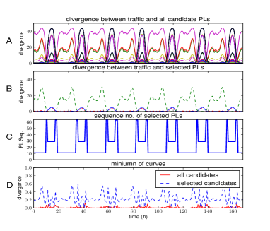
For the model-free method, there are $64$ candidate model-free PLs. The model-free divergence between each window and each candidate PL is a periodic function of time, too. Some PLs have smaller divergence during the day and some others have smaller divergence during the night (cf. Fig. 3A). However, no PL has small divergence for all windows. $3$ PLs out of the 64 candidates are selected when the detection threshold is $\lambda=0.6$ (cf. Fig. 3B). The 3 selected PLs are active during day, night, and the transitional time, respectively (cf. Fig. 3C for the active PLs of all windows). For all windows, the model-free generalized divergence between $\mathcal{G}_{ref}$ and all candidate PLs is very close to the divergence between $\mathcal{G}_{ref}$ and only the selected PLs (Fig. 3D). The difference is relatively larger during the transitional time between day and night. This is because the network is more dynamic during this transitional time, thus, more PLs are required to represent the network accurately.

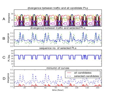
For the model-based method, there are 64 candidate model-based PLs, too. Similar to the model-free method, the model-based divergence between all candidate PLs and flows in each window in $\mathcal{G}_{ref}$ is periodic (Fig. 4A) and there is no PL that can represent all the reference data $\mathcal{G}_{ref}$. 2 PLs are selected when $\lambda=0.4$ (Fig. 4B). One PL is active during the transitional time and the other is active during the stationary time, which consists of both day and night (Fig. 4C). As before, the divergence between each $\mathcal{G}_{ref}^{i}$ and all candidate PLs is similar to the divergence between $\mathcal{G}_{ref}^{i}$ and just the selected PLs (Fig. 4D).

The results show that the PL refinement procedure is effective and the refined family of PLs is meaningful. Each PL in the refined family of the model-free method corresponds to a “pattern of normal behavior,” whereas, each PL in the refined family of the model-based method describes the transition among the “patterns”. This information is useful not only for anomaly detection but also for understanding the normal traffic in dynamic networks.

IV-B Comparison with vanilla stochastic methods

Figure 5: Comparison of vanilla and robust methods. (A), (B) show detection results of vanilla and robust model-free methods and (C), (D) show detection results of vanilla and robust model-based methods. The horizontal lines indicate the detection threshold.

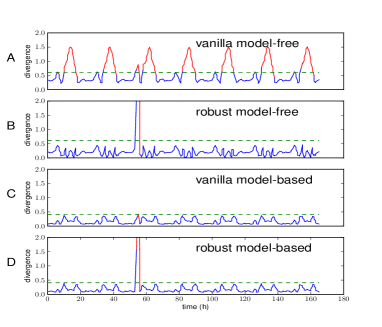
We compared the performance of our robust model-free and model-based method with their vanilla counterparts ([5, 18]) in detecting anomalies. In the vanilla methods, all reference traffic $\mathcal{G}_{ref}$ is used to estimate a single PL. We used all methods to monitor the server SRV for one week (168 hours).

We considered an anomaly in which node $CT2$ increases the mean flow size by $30\%$ at 59h and the increase lasts for 80 minutes before the mean returns to its normal value. This type of anomaly could be associated with a situation when attackers try to exfiltrate sensitive information (e.g., user accounts and passwords) through SQL injection [19].

For all methods, the window size is $w_{s}=2000s$ and the interval $h=2000s$. The quantization parameters are equal to those in the procedure for analyzing the reference traffic $\mathcal{G}_{ref}$. The simulation results show that the robust model-free and model-based methods perform better than their vanilla counterparts for both types of normal traffic patterns (Fig. 5).

The diurnal pattern has large influence on the results of the vanilla methods. For both the vanilla and the robust model-free methods, the detection threshold $\lambda$ equals 0.6. The vanilla model-free method reports all night traffic (between 3 am to 11 am) as anomalies (Fig. 5A). The reason is that the night traffic is lighter than the day traffic, so the PL calculated using all of $\mathcal{G}_{ref}$ is dominated by the day pattern, whereas the night pattern is underrepresented. In contrast, because both the day and the night pattern is represented in the refined family of PLs (Fig. 3B), the robust model-free method is not influenced by the fluctuation of normal traffic and successfully detects the anomaly (Fig. 5B).

The diurnal pattern has similar effects on the model-based methods. When the detection threshold $\lambda$ equals 0.4, the anomaly is barely detectable using the vanilla model-based method (Fig. 5C). Similar to the vanilla model-free method, the divergence is higher during the transitional time because the transition pattern is underrepresented in the PL calculated using all of $\mathcal{G}_{ref}$. Again, the robust model-based method is superior because both the transition pattern and the stationary pattern are well represented in the refined family of PLs (Fig. 5D).

V Conclusions

The statistical properties of normal traffic are time-varying for many networks. We propose a robust model-free and a robust model-based method to perform host-based anomaly detection in those networks. Our methods can generate a more complete representation of the normal traffic and are robust to the non-stationarity in networks.

References

- [1] M. Roesch et al., “Snort-lightweight intrusion detection for networks,” in Proceedings of the 13th USENIX conference on System administration. Seattle, Washington, 1999, pp. 229–238.
- [2] V. Paxson, “Bro: a system for detecting network intruders in real-time,” Computer networks, vol. 31, no. 23, pp. 2435–2463, 1999.
- [3] P. Barford, J. Kline, D. Plonka, and A. Ron, “A signal analysis of network traffic anomalies,” in Proceedings of the 2nd ACM SIGCOMM Workshop on Internet measurment. ACM, 2002, pp. 71–82.
- [4] W. Lu and A. a. Ghorbani, “Network Anomaly Detection Based on Wavelet Analysis,” EURASIP Journal on Advances in Signal Processing, vol. 2009, no. 1, p. 837601, 2009.
- [5] I. C. Paschalidis and G. Smaragdakis, “Spatio-temporal network anomaly detection by assessing deviations of empirical measures,” Networking, IEEE/ACM Transactions on, vol. 17, no. 3, pp. 685–697, 2009.
- [6] R. P. Lippmann, D. J. Fried, I. Graf, J. W. Haines, K. R. Kendall, D. McClung, D. Weber, S. E. Webster, D. Wyschogrod, R. K. Cunningham et al., “Evaluating intrusion detection systems: The 1998 darpa off-line intrusion detection evaluation,” in DARPA Information Survivability Conference and Exposition, 2000. DISCEX’00. Proceedings, vol. 2. IEEE, 2000, pp. 12–26.
- [7] A. Dembo and O. Zeitouni, Large Deviations Techniques and Applications, 2nd ed. NY:Spring-Verlag, 1998.
- [8] N. Leavitt, “Network-usage changes push internet traffic to the edge,” Computer, pp. 13–15, 2010.
- [9] K. Thompson, G. J. Miller, and R. Wilder, “Wide-area Internet traffic patterns and characteristics,” Network, IEEE, vol. 11, no. 6, pp. 10–23, 1997.
- [10] A. King, B. Huffaker, A. Dainotti, and K. C. Claffy, “A coordinated view of the temporal evolution of large-scale Internet events,” Computing, pp. 53–65, Jan. 2013.
- [11] Sandvine, “Global internet phenomena report,” https://www.sandvine.com/downloads/general/global-internet-phenomena/2013/sandvine-global-internet-phenomena-report-1h-2013.pdf, 2013.
- [12] W. Hoeffding, “Asymptotically optimal tests for multinomial distributions,” Ann. Math. Statist., vol. 36, pp. 369–401, 1965.
- [13] I. C. Paschalidis and D. Guo, “Robust and distributed stochastic localization in sensor networks: Theory and experimental results,” ACM Transactions on Sensor Networks, vol. 5, no. 4, 2009.
- [14] Cisco System, “Cisco netflow,” http://en.wikipedia.org/wiki/NetFlow, 2012.
- [15] J. Wang, “SADIT: Systematic Anomaly Detection of Internet Traffic,” http://people.bu.edu/wangjing/open-source/sadit/html/index.html, 2012.
- [16] J. Sommers, R. Bowden, B. Eriksson, P. Barford, M. Roughan, and N. Duffield, “Efficient network-wide flow record generation,” pp. 2363–2371, 2011.
- [17] A. Technologies, “The Net Usage Index by Industry,” http://www.akamai.com/html/technology/nui/industry/index.html, 2013.
- [18] R. Locke, J. Wang, and I. Paschalidis, “Anomaly detection techniques for data exfiltration attempts,” Center for Information & Systems Engineering, Boston University, 8 Saint Mary’s Street, Brookline, MA, Tech. Rep. 2012-JA-0001, June 2012.
- [19] M. Stampar, “Data Retrieval over DNS in SQL Injection Attacks,” arXiv preprint arXiv:1303.3047, 2013. [Online]. Available: http://arxiv.org/abs/1303.3047