Abstract

We present a Scan Method analysis of the allowed region of the $\overline{\rho}$ - $\overline{\eta}$ plane using the latest input measurements of CKM matrix elements, $\sin 2\beta$, $B^{0}_{d,s}$ mixing, $\epsilon_{K}$, $\alpha$ and $\gamma$. In this approach, we make no assumptions as to the distribution of theory uncertainties; rather, we scan over the range of plausible theoretical uncertainties and determine confidence level contours in the $\overline{\rho}$ -$\overline{\eta}$ plane. We determine $\alpha$ from branching fraction and $C\!P$  asymmetry measurements of $B$ decays to all light pseudoscalar-pseudoscalar, pseudoscalar-vector, vector-vector, and $a_{1}$-pseudoscalar mesons and determine $\gamma$ from $D^{(*)}K^{(*)},~{}D^{(*)}\pi$ and $D\rho$ modes, thereby including correlations between the angles of the unitarity triangle. We parameterize the individual decay amplitudes in terms of color-allowed tree, color-suppressed tree, gluing penguin, singlet penguin, electroweak penguin, as well as $W$-exchange and $W$-annihilation amplitudes. Our procedure accounts for all correlations among the fitted CKM parameters $(\overline{\rho},\overline{\eta},A$ and $\lambda$). The data are consistent with the Standard Model with no need for new physics contributions. We also examine example wall plots , i.e., projections of sensitive parameters showing correlations among them and regions of preferred theoretical parameters.

1 Introduction

The phase of the CKM matrix is responsible for $C\!P$ violation in the Standard Model (SM) [1]. Unitarity relations of the CKM matrix provide an excellent laboratory to test this prediction. The relation $V^{*}_{ub}V_{ud}+V^{*}_{cb}V_{cd}+V^{*}_{tb}V_{td}=0$ is particularly useful since, in the Wolfenstein parametrization [2], it represents a triangle in the $\overline{\rho}-\overline{\eta}$ plane. For this test, many measurements in the $B$ and $K$ systems can be combined. We perform the test with the SCAN Method [3], a frequentist technique in which we make no assumptions as to the distribution of theory uncertainties of lattice parameters and $|V_{ub}|$ and $|V_{cb}|$; rather, we scan over them using grid or MC methods. We determine confidence level (CL) contours in the $\overline{\rho}-\overline{\eta}$ plane and test the hypothesis that the SM is correct using a $\chi^{2}$ test compared to the alternative that the SM is incorrect.

2 Fit Methodology

We perform baseline fits in which we combine measurements of CKM matrix elements, $B\overline{B}$ mixing, $C\!P$ violation in the kaon system and angles of the unitarity triangle in the $\chi^{2}$.

$$\chi^{2}(\overline{\rho},\overline{\eta},p_{i},t_{j})= \Bigl{(}\frac{\langle\Delta m_{B}{{}_{d,s}}\rangle-\Delta m_{B_{d,s}}(\overline{\rho},\overline{\eta},p_{i},t_{j})}{\sigma_{\Delta m_{B_{d,s}}}}\Bigr{)}^{2}+\Bigl{(}\frac{\langle|V_{cb,ub,ud,us}|\rangle-|V_{cb,ub,ud,us}|(\overline{\rho},\overline{\eta},p_{i},t_{j})}{\sigma_{|V_{cb,ub,ud,us}|}}\Bigr{)}^{2}$$

$$+ \Bigl{(}\frac{\langle|\epsilon_{K}|\rangle-\epsilon_{K}(\overline{\rho},\overline{\eta},p_{i},t_{j})}{\sigma_{\epsilon_{K}}}\Bigr{)}^{2}+\Bigl{(}\frac{\langle S_{\psi K^{0}}\rangle-\sin 2\beta(\overline{\rho},\overline{\eta},p_{i})}{\sigma_{S_{\psi K^{0}}}}\Bigr{)}^{2}+\Bigl{(}\frac{\langle\alpha\rangle-\alpha(\overline{\rho},\overline{\eta},p_{i})}{\sigma_{\alpha}}\Bigr{)}^{2}$$

$$+ \Bigl{(}\frac{\langle\gamma\rangle-\gamma(\overline{\rho},\overline{\eta},p_{i})}{\sigma_{\gamma}}\Bigr{)}^{2}+\sum_{k}\Bigl{(}\frac{\langle{\cal M}_{k}\rangle-{\cal M}_{k}(p_{i})}{\sigma_{{\cal M}_{k}}}\Bigr{)}^{2}+\sum_{n}\Bigl{(}\frac{\langle{\cal T}_{n}\rangle-{\cal T}_{n}(p_{i},t_{j})}{\sigma_{{\cal T}_{n}}}\Bigr{)}^{2}.$$ (1)

Here, ${\cal M}_{k}$ terms represent other measurements such as charm and top quark masses and ${\cal T}_{n}$ terms represent lattice parameters that have theory uncertainties. We also perform “full fits” in which we use as inputs the measurements that determine $\alpha$ and $\gamma$ rather than the derived values of these angles. Confidence regions are determined by comparing $\chi^{2}$ values with a critical value instead of looking for a change in $\chi^{2}$. The algorithm for a $(1-\alpha_{c})$ confidence region in $d$ dimensions of a $p$ dimensional parameter space with $n$ measurements is as follows: We first determine the acceptance region, at the $\alpha_{c}$ significance level, by determining the critical value $\chi_{c}^{2}$ such that $P(\chi^{2}\geq\chi_{c}^{2};n-p+d|H_{0})\geq\alpha_{c}$, where $H_{0}$ is the hypothesis of the SM, and $n-p+d$ is the number of degrees of freedom. The confidence region is then given by all those points in the $d$ dimensional parameter subspace for which $\chi^{2}\leq\chi^{2}_{c}$, under $H_{0}$.

3 Fit Results in the $\overline{\rho}-\overline{\eta}$ Plane

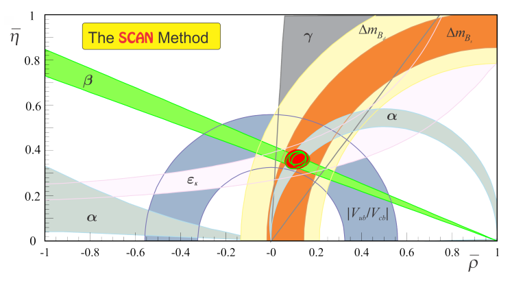
In the baseline fits, we fit 23 measurements ($|V_{ud}|,|V_{us}|,|V_{cb}|$, $|V_{ub}|,|V_{cs}|,|V_{cd}|,|V_{tb}|$, $\epsilon_{K},\Delta m_{d}$, $\Delta m_{s},\sin 2\beta$, $\alpha$, $\gamma$, ${\cal B}(B\ \rightarrow\tau\nu),f_{B_{s}},f_{B_{s}}/f_{B_{d}},B_{B_{s}},B_{B_{s}}/B_{B_{d}},B_{K},m_{t},m_{c},\tau_{B_{d}},\tau_{B_{s}})$ listed in Tables 1 and 2 to 13 parameters $(\overline{\rho},\overline{\eta}$, $A,\lambda,f_{B_{s}},f_{B_{s}}/f_{B_{d}},B_{B_{s}},B_{B_{s}}/B_{B_{d}},B_{K},m_{t},m_{c},\tau_{B_{d}},\tau_{B_{s}})$. The PDG [4] uses scaling factors of 2.6 and 2.0 for averaging $|V_{ub}|$ and $|V_{cb}|$ results from inclusive and exclusive modes, respectively. This procedure increases all errors. Figure 1 (left) shows the overlay of $1-\alpha_{c}$ confidence level (CL) contours of all accepted fits.

Table 1: Measurement inputs.

Input	Value	Ref	Input	Value	Ref
$|V_{cb}|$	$(4.09\pm 0.069\pm 0.09)\times 10^{-2}$	[4]	$m_{t}$	$(173.07\pm 0.88)\rm GeV/c^{2}$	[4]
$|V_{ub}|$	$(4.15\pm 0.31\pm 0.39)\times 10^{-3}$	[4]	$m_{c}$	$(1.275\pm 0.025)\rm GeV/c^{2}$	[4]
$|V_{us}|$	$0.2252\pm 0.0009$	[5]	$\Delta m_{d}$	$(0.510\pm 0.003)\rm ps^{-1}$	[4]
$|V_{ud}|$	$0.97425\pm 0.00022$	[5]	$\Delta m_{s}$	$(17.761\pm 0.022)\rm ps^{-1}$	[4]
$|V_{cd}|$	$0.23\pm 0.11$	[4]	$\epsilon_{K}$	$(2.228\pm 0.0011)\times 10^{-3}$	[4]
$|V_{cd}|$	$1.006\pm 0.023$	[4]	$\sin 2\beta$	$0.682\pm 0.019$	[4]
$|V_{tb}|$	$0.97\pm 0.08$	[4]	$\alpha$	$85.1^{+2.2^{\circ}}_{-2.0}$	†
${\cal B}(B\rightarrow\tau\nu)$	$(1.15\pm 0.23)\times 10^{-4}$	[6]	$\gamma$	$78.9^{+6.6}_{-10.3}$	‡

Table 2: Lattice parameters and QCD parameters.

Lattice	Value	Ref	QCD	Value	Ref
parameter			parameter
$f_{B_{s}}$	$(228.66\pm 2.0\pm 5.5)\rm MeV$	[7]	$\eta_{cc}$	$1.39\pm 0.35$	[8, 9]
$f_{B_{s}}/f_{B_{d}}$	$1.205\pm 0.0086\pm 0.0188$	[7]	$\eta_{tc}$	$0.47\pm 0.04$	[8, 10]
$B_{B_{s}}$	$1.311\pm 0.046\pm 0.076$	[7]	$\eta_{tt}$	$0.5765\pm 0.0065$	[8, 11]
$B_{B_{s}}/B_{B_{d}}$	$1.053\pm 0.040\pm 0.064$	[7]	$\eta_{b}$	$0.551\pm 0.007$	[11]
$B_{K}$	$0.7584\pm 0.0020\pm 0.019$	[7]

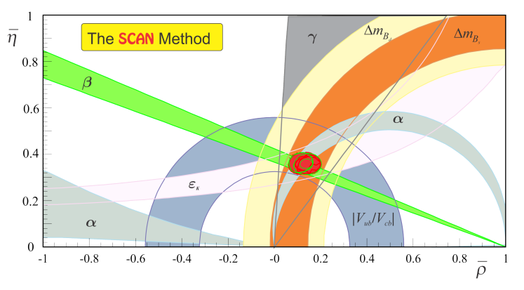
We also perform “full fits” in which we use 256 branching fraction and $C\!P$ asymmetry measurements instead of the $\alpha$ and $\gamma$ direct inputs. These fits, with 114 parameters, uniquely among the procedures in common use [12, 13] account for possible correlations among $\alpha,\beta$ and $\gamma$. We currently include all branching fraction and $C\!P$ asymmetry measurements of $B$ to pseudoscalar-pseudoscalar ($PP$), pseudoscalar-vector ($PV$), vector-vector ($VV$) and $a_{1}$-pseudoscalar ($a_{1}P$) modes to determine $\alpha$. We include tree, color-suppressed tree, penguin, singlet penguin, $W$-exchange, $W$-annihilation, and EW penguin amplitudes (up to $\lambda^{3}$ beyond leading order), as well as $SU(3)$ corrections in defining the amplitudes. We parametrize the observables using the Gronau-Rosner approach [14, 15, 16, 17, 18, 19]. The amplitude ratios and $C\!P$ asymmetry measurements of $B^{\pm}\rightarrow DK^{\pm},~{}B^{\pm}\rightarrow D^{*}K^{\pm}$ and $B\rightarrow DK^{*\pm}$ modes determine $\gamma$, while those of $B^{\pm}\rightarrow D\pi^{\pm},~{}B^{\pm}\rightarrow D^{*}\pi^{\pm}$ and $B\rightarrow D\rho^{\pm}$ modes determine $\sin(2\beta+\gamma)$. Figure 1 (right) shows an overlay of $1-\alpha_{c}$  CL contours of all successful full fits in $\overline{\rho}-\overline{\eta}$ plane.

Figure 1: Contours at $1-\alpha_{c}$ CL in the $\overline{\rho}-\overline{\eta}$ plane for baseline fits (top) and full fits (bottom).

Table 3: $1-\alpha_{c}$  CL ranges for Unitarity Triangle parameters from baseline fits and full fits.

Parameter	Baseline Fit	Baseline Fit	Full Fit
	without $B\rightarrow\tau\nu$	with $B\rightarrow\tau\nu$	without $B\rightarrow\tau\nu$
$\overline{\rho}$	$0.069-0.144$	$0.073-0.145$	$0.081-0.126$
$\overline{\eta}$	$0.320-0.395$	$0.324-0.396$	$0.331-0.375$
$\beta~{}[^{\circ}]$	$19.4-24.2$	$19.7-24.3$	$20.1-22.8$
$\alpha~{}[^{\circ}]$	$79.8-90.2$	$80.0-90.1$	$81.8-88.2$
$\gamma~{}[^{\circ}]$	$68.0-78.7$	$68.0-78.2$	$70.3-77.0$

4 Extraction of $\alpha$ and $\gamma$

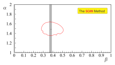
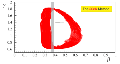
We use 181 branching fraction and $C\!P$ asymmetry measurements of $B\rightarrow PP$, $B\rightarrow PV$, $B\rightarrow VV$, and $B\rightarrow a_{1}P$ modes  [6]to fit 94 parameters and determine the $\alpha-\beta$ contour $@(1-\alpha_{c})$ CL shown in Fig. 2 (left). The central value of $\beta$ is consistent with the measured world average of $\beta=(21.5^{+0.8}_{-0.7})^{\circ}$ extracted from $\sin 2\beta$ measured in $b\rightarrow c\overline{c}s$ modes. Further, we use 56 branching fraction and $C\!P$ asymmetry measurements of $B^{\pm}\rightarrow D^{(*)}K^{\pm},DK^{*\pm},D^{(*)}\pi$, and $D^{-}\rho^{+}$ modes  [6] analyzed with the GLW [20, 21], ADS [22, 23] and GGSZ [24] methods to fit 19 parameters and plot $\gamma-\beta$ contours  $@(1-\alpha_{c})$  CL, which are shown in Fig. 2 (right). Since the contours depend on $|V_{ub}/V_{cb}|$, we explicitly scan over the ratio. The central values for $\beta$ again agree with the world average measured in $b\rightarrow c\overline{c}s$ decay modes.

Figure 2: The $1-\alpha_{c}$  CL contour in the $\alpha-\beta$ plane from fits to branching fractions and $C\!P$ asymmetries of $B\rightarrow PP,~{}PV,~{}VV,~{}a_{1}P$ modes (left) and $1-\alpha_{c}$  CL contours in the $\gamma-\beta$ plane from fits to $B^{\pm}\rightarrow D^{(*)}K^{\pm},DK^{*\pm},D^{(*)}\pi$, and $D^{-}\rho^{+}$ modes (right). The individual $\gamma-\beta$ contours result from a scan over $|V_{ub}/V_{cb}|$. The grey-shaded band shows the world average of $\beta$ measured in $b\rightarrow c\overline{c}s$ modes.

Table 4: Determination of the angle $\alpha$ from fits to branching fractions and $C\!P$ asymmetries of $B\rightarrow PP,~{}PV,~{}VV$, and $a_{1}P$ modes and determination of $\gamma$ from rate and $C\!P$ asymmetry measurements of $B^{\pm}\rightarrow D^{(*)}K^{\pm}$, $B^{\pm}\rightarrow DK^{*\pm}$, $B\rightarrow D^{(*)}\pi$, and $B^{0}\rightarrow D^{-}\rho^{+}$ modes.

Mode	$\alpha[^{\circ}]$	$\beta[^{\circ}]$	$\gamma[^{\circ}]$
$B\rightarrow PP+PV+VV+a_{1}P$	$85.1^{+2.2}_{-2.1}$	$21.8^{+1.6}_{-2.1}$
$B\rightarrow D^{(*)}h$		$22.8^{+7.7}_{-2.0}$	$78.9^{+6.6}_{-10.3}$

5 Wall Plots

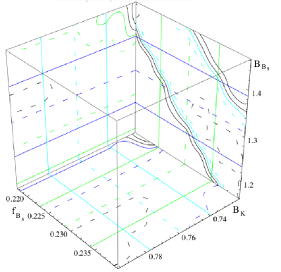
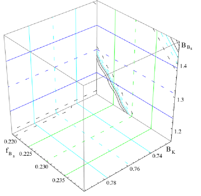
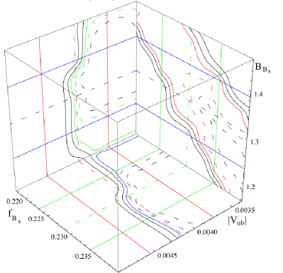
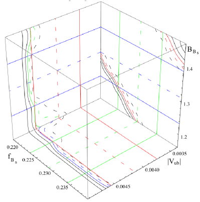
We construct wall plots to display the correlations among sets of three out of the seven parameters with large theory uncertainties. To study the impact of the remaining parameters on two parameters displayed, we impose different constraints on the other displayed and undisplayed parameters. These studies clearly show that certain regions of the theory parameters are favored by the data while others are not. As an example, Figure 3 shows correlations for $B_{B_{s}}$ versus $B_{K}$ versus $f_{B_{s}}$ (top) and $B_{B_{s}}$ versus $|V_{ub}|$ versus $f_{B_{s}}$ (bottom) for $68\%$ CL (left) and $1-\alpha_{c}$ CL (right). Orthogonal solid lines in each plane show the $\pm 1\delta$ theory error range. Outer black contours result from a probability requirement of $>\!32\%$ or $>\!5\%$. Inner black contours result from a $\pm 1\delta$ requirement on all undisplayed parameters while colored solid contours result from a $\pm 1\delta$ requirement on the out-of-plane variable. Constraining the out-of-plane variable to its central value yields the colored dashed contours while the black dashed contours result from constraining undisplayed variables to their central values. The plots show that larger values of $B_{K}$ and $f_{B_{s}}$ and smaller values of $|V_{ub}|$ are favored.

Figure 3: Wall plots for $B_{B_{s}}$ versus $B_{K}$ versus $f_{B_{s}}$ (top) and $B_{B_{s}}$ versus $|V_{ub}|$ versus $f_{B_{s}}$ (bottom) for $68\%$ contours (left) and $1-\alpha_{c}$ contours (right).

6 Conclusion

Baseline fits and full fits performed with the SCAN method yield results that are in good agreement with the SM without making any assumptions about the distribution of theory uncertainties as is done for $\rm UT_{fit}$ [12] and CKMfitter [13] analyses. The full fits how a slightly larger allowed region in the $\overline{\rho}-\overline{\eta}$ plane. They account for correlations among the observables $\alpha$, $\beta$ and $\gamma$. These correlations, however, are ignored in $\rm UT_{fit}$ and CKMfitter analyses. Wall plots allow the determination of whether any potential SM discrepancy originates from the values of theory parameters or from experimental measurements. The measurements prefer larger values of $B_{K}$ and $f_{B_{s}}$ and smaller values of $|V_{ub}|$.

7 Acknowledgments

This work is supported in part by the U. S. Department of Energy under Grant DE-FG02-92-ER40701 and by the NFR (Norway).

References

- [1] M. Kobayashi and T. Maskawa, Prog. Theor. Phys. 49, 652 (1973).
- [2] L. Wolfenstein, Phys. Rev. Lett. 51, 1945 (1983).
- [3] G. Eigen , Phys. Rev. D 89, 033004 (2014) [hep-ex/1301.5867].
- [4] J. Beringer et al. [Particle Data Group Collaboration], Phys. Rev. D 86, 010001 (2012).
- [5] G. Colangelo , Eur. Phys. J. C 71, 1695 (2011) [arXiv:1011.4408 [hep-lat]].
- [6] Y. Amhis et al. [Heavy Flavor Averaging Group Collaboration], arXiv:1207.1158 [hep-ex].
- [7] J. Laiho, E. Lunghi and R. S. Van de Water, Phys. Rev. D 81, 034503 (2010) [hep-ph/0910.2928]; http://mypage.iu.edu/elunghi/webpage/LatAves.
- [8] F. J. Gilman and M. B. Wise, Phys. Rev. D 27, 1128 (1983).
- [9] S. Herrlich and U. Nierste, Nucl. Phys. B 419, 292 (1994) [hep-ph/9310311].
- [10] S. Herrlich and U. Nierste, Nucl. Phys. B 476, 27 (1996) [hep-ph/9604330].
- [11] A. J. Buras, M. Jamin and P. H. Weisz, Nucl. Phys. B 347, 491 (1990).
- [12] M. Bona et al. [UTfit Collaboration], JHEP 0803, 049 (2008), arXiv:0707.0636 [hep-ph]; updates at http://ckmfitter.in2p3.fr/.
- [13] J. Charles et al. [CKMfitter Group Collaboration], Eur. Phys. J. C 41, 1 (2005), [hep-ph/0406184].
- [14] M. Gronau , Phys. Rev. D 50, 4529 (1994) [hep-ph/9404283].
- [15] M. Gronau, D. Pirjol and T. M. Yan, Phys. Rev. D 60, 034021 (1999) [Erratum-ibid. D 69, 119901 (2004)] [hep-ph/9810482].
- [16] A. S. Dighe , Phys. Rev. D 57, 1783 (1998) [hep-ph/9709223].
- [17] M. Gronau and J. L. Rosner, Phys. Rev. D 61, 073008 (2000) [hep-ph/9909478].
- [18] M. Gronau, Phys. Rev. D 62, 014031 (2000) [hep-ph/9911429].
- [19] M. Beneke , Phys. Lett. B 638, 68 (2006) [hep-ph/0604005].
- [20] M. Gronau and D. London, Phys. Lett. B 253, 483 (1991).
- [21] M. Gronau and D. Wyler, Phys. Lett. B 265, 172 (1991).
- [22] D. Atwood, I. Dunietz and A. Soni, Phys. Rev. Lett. 78, 3257 (1997) [hep-ph/9612433].
- [23] D. Atwood, I. Dunietz and A. Soni, Phys. Rev. D 63, 036005 (2001) [hep-ph/0008090].
- [24] A. Giri , Phys. Rev. D 68, 054018 (2003) [hep-ph/0303187].