label.switching: An R Package for Dealing with the Label Switching Problem in MCMC Outputs

Panagiotis Papastamoulis label.switching: An R Package for dealing with the Label Switching problem in MCMC outputs label.switching: Relabelling MCMC outputs Label switching is a well-known and fundamental problem in Bayesian estimation of mixture or hidden Markov models. In case that the prior distribution of the model parameters is the same for all states, then both the likelihood and posterior distribution are invariant to permutations of the parameters. This property makes Markov chain Monte Carlo (MCMC) samples simulated from the posterior distribution non-identifiable. In this paper, the label.switching package is introduced. It contains one probabilistic and seven deterministic relabelling algorithms in order to post-process a given MCMC sample, provided by the user. Each method returns a set of permutations that can be used to reorder the MCMC output. Then, any parametric function of interest can be inferred using the reordered MCMC sample. A set of user-defined permutations is also accepted, allowing the researcher to benchmark new relabelling methods against the available ones. Label switching, mixture models, hidden Markov, MCMC, R Label switching, mixture models, hidden Markov, MCMC, R Panagiotis Papastamoulis
Department of Statistics and Insurance Science
University of Piraeus
Greece
E-mail:

1 Introduction

Mixture and hidden Markov models are a powerful tool for modelling a wide range of phenomena and they have been extremely useful in many fields (McLachlan:00; Fruhwirth:06). Such applications include the presence of unobserved heterogeneity in the studied population or the approximation of unknown distributions, after deciding the proper number of latent states (or components). The complex nature of such models can be simplified by decomposing the model into simpler structures using latent (unobserved) variables. Data augmentation (tanner) is a standard technique exploited both by the EM algorithm (Dempster:77) as well as the Gibbs sampler (gelfand).

Under a Bayesian perspective, MCMC estimation of the posterior distribution of such models is quite straightforward. Gibbs sampling enables the simulation of a Markov chain from the joint posterior distribution of model parameters and latent variables. Nevertheless, the likelihood of such models is invariant to permutations of the components’ labels and this property gives rise to the label switching phenomenon (Redner; jasra). It is well known that the presence of the label switching phenomenon in an MCMC sample serves as a necessary condition for the convergence of the chain to the target distribution. On the other hand, the presence of the phenomenon complicates the posterior inference.

Early attempts to solve the label switching were focused on the use of suitable identifiability constraints (diebolt; Richardson:97; Fruhwirth:01). However, it is not always possible to find such constraints and in most cases a single identifiability constraint will not respect the geometry of the posterior distribution. For these reasons, a variety of different relabelling algorithms has been proposed.

The purpose of this study is to introduce the label.switching package, available from the Comprehensive R Archive Network at http://CRAN.R-project.org/package=label.switching, which can be used in order to deal with the label switching problem using various algorithms that have been proposed to the related literature. More specifically, the label.switching package consists of eight relabelling methods: ordering constraints, the Kullback-Leibler based algorithm (stephens), the pivotal reordering algorithm (Marin:05; Marin:07), the default and iterative versions of ECR algorithm (Papastamoulis:10; Rodriguez; Papastamoulis:13; Papastamoulis:14), the probabilistic relabelling algorithm (sperrin) and the data-based algorithm (Rodriguez).

In many instances, it is required to draw meaningful comparisons between different relabelling algorithms or to benchmark novel methods against the existing ones. Both issues are addressed to the label.switching package. At first, the output of each relabelling method is reported in a way that the resulting single best clusterings are comparable among them. Moreover, the user can provide alternative sets of permutations arising from any (consistent) relabelling procedure and directly compare them to the available methods.

The rest of the paper is organised as follows. A short introduction to mixture models is given at Section 2. Section 2.1 discusses the label switching phenomenon and some helpful notation is introduced. The relabelling algorithms contained at the label.switching package are briefly reviewed at Section 3. Section 4 gives an overview of the package and the most important functions are described in detail. The practical implementation of the package is illustrated at Section 5 using two real datasets from classic mixture and hidden Markov models, as well as two simulated datasets from mixtures of bivariate normal distributions. The paper concludes at Section LABEL:sec:discussion.

2 Mixture models

Let $\boldsymbol{x}=(x_{1},\ldots,x_{n})$ denote a sample of $n$ (possibly multivariate) observations. Assume that $\boldsymbol{z}=(z_{1},\ldots,z_{n})$ is an unobserved (latent) sequence of state variables, with $z_{i}\in\{1,\ldots,K\}$, where $K>1$ denotes a known integer. Let $f$ denotes a member of a parametric family of distributions $f\in\mathcal{F}_{\Theta}:=\{f(\cdot|\theta):\theta\in\Theta\}$, with $\Theta\subseteq\mathbb{R}^{d}$, for some $d\geqslant 1$. Conditionally to $z_{i}$ and a vector of parameters $\boldsymbol{\theta}=(\theta_{1},\ldots,\theta_{K})$ the observations are distributed according to

$$x_{i}|(z_{i}=k,\theta_{k})\sim f(\cdot|\theta_{k}),\quad k=1,\ldots,K$$ (1)

for $i=1,\ldots,n$.

Assume that $z_{i}$, $i=1,\ldots,n$, are independent random variables following the multinomial distribution with weights $\boldsymbol{w}:=(w_{1},\ldots,w_{K})$, that is,

$$P(z_{i}=k|w_{k})=w_{k},\quad k=1,\ldots,K$$ (2)

independently for $i=1,\ldots,n$ and $\boldsymbol{w}\in\boldsymbol{W}:=\{w_{k}>0,k=1,\ldots,K-1:\sum_{k=1}^{K-1}w_{k}<1;w_{K}:=1-\sum_{k=1}^{K-1}w_{k}\}$. The marginal distribution of $x_{i}$ is a finite mixture of $K$ distributions:

$$x_{i}|\boldsymbol{\theta},\boldsymbol{w}\sim\sum_{k=1}^{K}w_{k}f(x_{i}|\theta_{k}).$$ (3)

The conditional probability for observation $i$ to belong to component $k$ can be expressed as

$$p_{ik}=\frac{w_{k}f(x_{i}|\theta_{k})}{w_{1}f(x_{i}|\theta_{1})+\ldots+w_{K}f(x_{i}|\theta_{K})},\quad i=1,\ldots,n;\quad k=1\ldots,K.$$ (4)

We will refer to Equation 4 with the term classification probabilities. The observed likelihood of the mixture is defined as:

$$L(\boldsymbol{\theta},\boldsymbol{w};\boldsymbol{x})=\prod_{i=1}^{n}\sum_{k=1}^{K}w_{k}f(x_{i}|\theta_{k}).$$ (5)

The complete likelihood of the model is written as:

$$L_{c}(\boldsymbol{\theta},\boldsymbol{w};\boldsymbol{x},\boldsymbol{z})=\prod_{i=1}^{n}w_{z_{i}}f(x_{i}|\theta_{z_{i}}).$$ (6)

2.1 Label switching phenomenon

Let $\mathcal{T}_{K}$ denote the set of permutations of $\{1,\ldots,K\}$. For any $\boldsymbol{\tau}=(\tau_{1},\ldots,\tau_{K})\in\mathcal{T}_{K}$ define the corresponding permutation of the component specific parameters, weights and allocations as: $\boldsymbol{\tau}\boldsymbol{\theta}:=(\theta_{\tau_{1}},\ldots,\theta_{\tau_{K}})$, $\boldsymbol{\tau}\boldsymbol{w}:=(w_{\tau_{1}},\ldots,w_{\tau_{K}})$ and $\boldsymbol{\tau}\boldsymbol{z}:=(\tau_{z_{1}},\ldots,\tau_{z_{n}})$, respectively.

Notice now that the likelihood of the mixture model is invariant for any permutation of the parameters, that is,

$$L(\tau\boldsymbol{\theta},\tau\boldsymbol{w};\boldsymbol{x})=L(\boldsymbol{\theta},\boldsymbol{w};\boldsymbol{x}),$$ (7)

for all $\tau\in\mathcal{T}_{K}$, $\boldsymbol{\theta}\in\Theta$, $\boldsymbol{w}\in\boldsymbol{W}$. Let $p(\boldsymbol{\theta},\boldsymbol{w})$ denote the prior distribution of component specific parameters and weights of the model. It will be assumed that this prior is permutation invariant as well, that is,

$$p(\tau\boldsymbol{\theta},\tau\boldsymbol{w})=p(\boldsymbol{\theta},\boldsymbol{w}),$$ (8)

for all $\tau\in\mathcal{T}_{K}$, $\boldsymbol{\theta}\in\Theta$, $\boldsymbol{w}\in\boldsymbol{W}$. A typical choice (Richardson:97; Fruhwirth:01; Marin:05) for the prior of the component parameters is to assume that $\boldsymbol{\theta}\sim\prod_{k=1}^{K}p(\theta_{k})$, independently for $k=1,\ldots,K$, for a specific family of distributions $p(\cdot)$ which is common to all states. A common prior assumption on the mixture weights is a non-informative Dirichlet distribution.

Let $p(\boldsymbol{\theta},\boldsymbol{w}|\boldsymbol{x})\propto L(\boldsymbol{\theta},\boldsymbol{w};\boldsymbol{x})p(\boldsymbol{\theta},\boldsymbol{w})$ denotes the posterior distribution of the mixture model parameters. From Equations 7 and 8 it follows that the same invariance property holds for the posterior distribution, that is, $p(\tau\boldsymbol{\theta},\tau\boldsymbol{w}|\boldsymbol{x})=p(\boldsymbol{\theta},\boldsymbol{w}|\boldsymbol{x})$, for all $\tau\in\mathcal{T}_{K}$, $\boldsymbol{\theta}\in\Theta$, $\boldsymbol{w}\in\boldsymbol{W}$. This implies that all marginal densities of component specific parameters and weights are coinciding. Now, if a simulated output from any MCMC sampler has converged to the symmetric posterior distribution, the generated values will be switching between the symmetric high posterior density areas.

This behaviour is known as the label switching phenomenon and makes the generated MCMC sample non-identifiable. Hence, it is not straightforward to draw inference for any parametric function that depends on the labels of the components. In order to derive meaningful estimates, all simulated parameters should be switched to one among the $K!$ symmetric areas of the posterior distribution. This is done by applying suitable permutations of the labels $\{1,\ldots,K\}$ to each MCMC draw.

3 Algorithms

In this section we will describe the relabelling algorithms that are available to label.switching package. It consists of seven deterministic and one probabilistic relabelling method, as shown at Table 1. The third column describes the necessary input of the algorithms, while the input notation is described in detail at Table 2, where $m$ denotes the number of retained MCMC iterations.

For practical purposes it will be convenient to arrange all component specific parameters ($\boldsymbol{\theta}$) and weights/transition probabilities ($\boldsymbol{w}$) at a $K\times J$ matrix $\boldsymbol{\xi}$. The number of columns ($J$) of the global parameter vector $\boldsymbol{\xi}:=(\boldsymbol{\theta},\boldsymbol{w})$ is equal to the number of different types of parameters of the model. For example, if Equation 3 corresponds to a univariate normal mixture model, then there are $J=3$ different types: $\xi_{kj}$ denotes the mean ($j=1$), variance ($j=2$) and weight ($j=3$), respectively, for component $k=1,\ldots,K$. In case of a bivariate normal mixture, there are $J=6$ parameter types for each component: two parameters for the mean vector, two variances, one covariance and one weight.

In the sequel, we will assume that an augmented sample $(\boldsymbol{\xi}^{(t)},\boldsymbol{z}^{(t)})$, $t=1,\ldots,m$, has been generated by an MCMC algorithm. Moreover, let $p_{ik}^{(t)}$, $t=1,\ldots,m$, $k=1,\ldots,K$, $i=1,\ldots,n$ denote the corresponding classification probabilities across the MCMC run.

Function	Method	Input
aic	Ordering constraints	mcmc, constraint
dataBased	Data-based	z, x, K
ecr	ECR (default)	z, zpivot, K
ecr.iterative.1	ECR (iterative vs. 1)	z, K
ecr.iterative.2	ECR (iterative vs. 2)	z, K, p
pra	PRA	mcmc, pivot
stephens	Stephens	p
sjw	Probabilistic	mcmc, z, x, complete

Table 1: The available relabelling algorithms at label.switching package.

Object	Type	Dimension	Details
z	Array (integer)	$m\times n$	simulated allocation vectors
x	Array	$n\times d$	observed data
zpivot	Numeric (integer)	$n$	pivot allocation vector
p	Array (real)	$m\times n\times K$	classification probabilities
mcmc	Array (real)	$m\times K\times J$	simulated parameters
pivot	Array (real)	$K\times J$	pivot parameter
complete	Function	–	complete log-likelihood function

Table 2: Input notation for the relabelling algorithms.

3.1 Ordering constraints

Imposing an artificial identifiability constraint to the MCMC sample is the simplest approach to the label switching problem. In such a case, the simulated MCMC output is permuted according to the ordering of a specific parameter. However, this approach works well only in cases that the selected constraint is able to separate the symmetric posterior modes, which is rarely true.

Algorithm 1 (Ordering constraints).

1. Choose a specific parameter type $\xi_{s}$, $s=1,\ldots,J$.

2. For $t=1,\ldots,m$ find the permutation $\tau^{(t)}\in\mathcal{T}_{K}$ that $\xi_{\tau_{1}j}^{(t)}<\ldots<\xi_{\tau_{K}j}^{(t)}$.

3.2 Stephens’ method

One of the first principled solutions to the label switching problem was proposed by stephens. The idea behind Stephens’ algorithm is to make the permuted MCMC draws agree on the $n\times K$ matrix of classification probabilities. For this purpose, the Kullback-Leibler divergence between an averaged matrix of classification probabilities across the MCMC run and the classification matrix at each MCMC iteration is minimized at an iterative fashion. In general, Stephens’ algorithm is very efficient in terms of finding the correct relabelling, but its drawback is the need to store the $m\times n\times K$ matrix p of classification probabilities.

Algorithm 2 (Kullback-Leibler relabelling).

1. Choose $m$ initial permutations $\tau^{(t)}$ $t=1,\ldots,m$ (usually set to identity).

2. For $t=1,\ldots,m$, $k=1,\ldots,K$ calculate $q_{ik}:=\frac{1}{m}\sum_{t=1}^{m}p_{i\tau_{k}}^{(t)}$.

3. For $t=1,\ldots,m$ find a permutation $\tau^{(t)}\in\mathcal{T}_{K}$ that minimizes $\sum_{i=1}^{n}\sum_{k=1}^{K}p_{i\tau_{k}}^{(t)}\log\left(\frac{p_{i\tau_{k}}^{(t)}}{q_{ik}}\right)$.

4. If an improvement is made to $\sum_{t=1}^{m}\sum_{i=1}^{n}\sum_{k=1}^{K}p_{i\tau_{k}}^{(t)}\log\left(\frac{p_{i\tau_{k}}^{(t)}}{q_{ik}}\right)$ go to step 2, finish otherwise.

3.3 Pivotal reordering algorithm

The Pivotal Reordering Algorithm (PRA), proposed by Marin:05; Marin:07, is a very simple geometrically-based solution to the label switching. The idea is to permute all simulated MCMC samples of parameters so that they are maximizing their similarity to a pivot parameter vector, as the complete MAP estimate. This is done by selecting the permutation that minimizes the Euclidean distance between the pivot and the set of permuted parameter vectors at each MCMC iteration. In principle, this method is a data-driven way to apply an artificial identifiability constraint on the parameter space.

Algorithm 3 (Pivotal Reordering).

1. Define a pivot parameter vector: $\boldsymbol{\xi}^{*}=(\xi^{*}_{kj})$, $k=1,\ldots,K$, $j=1,\ldots,J$.

2. For $t=1,\ldots,m$ find a permutation $\tau^{(t)}\in\mathcal{T}_{K}$ that maximizes $\sum_{j=1}^{J}\sum_{k=1}^{K}\xi^{(t)}_{\tau_{k}j}\xi_{kj}^{*}$.

Note here that maximizing the dot product $\tau\boldsymbol{\xi}^{(t)}\cdot\boldsymbol{\xi}^{*}$ in step 2 is equivalent to minimizing the Euclidean distance between $\tau\boldsymbol{\xi}^{(t)}$ and $\boldsymbol{\xi}^{*}$.

3.4 ECR algorithms

ECR algorithm was originally proposed by Papastamoulis:10 and it is based on the idea that equivalent allocation vectors are mutually exclusive from the label switching solution. Two allocation vectors are called equivalent if the first one arises from the second by simply permuting its labels. ECR algorithm partitions the set of allocation vectors into equivalence classes and selects a representative from each class. Then, the permutation needed to be applied at a given MCMC iteration is determined by the one that reorders the corresponding allocations in order to become identical to the representative of its class.

In the default version of ECR algorithm (ecr), equivalence classes are determined using a pivot allocation vector zpivot. The pivot is selected by choosing a high-posterior density point, such as the complete or non-complete Maximum A Posteriori (MAP) estimate. Rodriguez tried to relax the dependence of ECR algorithm to a pivot and proposed two iterative versions (ecr.iterative.1 and ecr.iterative.2). The first algorithm is using as input only the simulated allocation variables and is initialized by a pivot selected at random. Then, the standard version of ECR is repeated until a fixed pivot has been found. Nevertheless, it is not guaranteed that this procedure will lead to a “good” pivot. The second iterative ECR algorithm requires the knowledge of classification probabilities across the MCMC run and it could be described as an allocation vectors version of Stephens’ algorithm. Of course the problem of storing the matrix p applies to this method as well. However, as it will be demonstrated in the applications, ecr.iterative.2 is significantly faster than stephens.

Algorithm 4 (ECR: default version).

1. Define a pivot allocation: $\boldsymbol{z}^{*}=(z^{*}_{1},\ldots,z^{*}_{n})$.

2. For $t=1,\ldots,m$ find a permutation $\tau^{(t)}\in\mathcal{T}_{K}$ that maximizes $\sum_{i=1}^{n}I(\tau z_{i}^{(t)}=z^{*}_{i})$.

Algorithm 5 (ECR: iterative version 1).

1. Choose $m$ initial permutations $\tau^{(t)}$, $t=1,\ldots,m$ (usually set to identity).

2. Update the pivot: $z^{*}_{i}=\mbox{mode}\{\tau z_{i}^{(t)};t=1,\ldots,m\}$, $i=1,\ldots,n$.

3. For $t=1,\ldots,m$ find a permutation $\tau^{(t)}\in\mathcal{T}_{K}$ that maximizes $\sum_{i=1}^{n}I(\tau z_{i}^{(t)}=z^{*}_{i})$.

4. If an improvement is made to $\sum_{t=1}^{m}\sum_{i=1}^{n}I(\tau z_{i}^{(t)}=z^{*}_{i})$ go to step 2, finish otherwise.

Algorithm 6 (ECR algorithm: iterative version 2).

1. Choose $m$ initial permutations $\tau^{(t)}$, $t=1,\ldots,m$ (usually set to identity).

2. Update the pivot: $z^{*}_{i}=\mbox{argmax}\{p_{i\tau_{k}}^{(t)};t=1,\ldots,m\}$, $i=1,\ldots,n$.

3. For $t=1,\ldots,m$ find a permutation $\tau^{(t)}\in\mathcal{T}_{K}$ that maximizes $\sum_{i=1}^{n}I(\tau z_{i}^{(t)}=z^{*}_{i})$.

4. If an improvement is made to $\sum_{t=1}^{m}\sum_{i=1}^{n}I(\tau z_{i}^{(t)}=z^{*}_{i})$ go to step 2, finish otherwise.

3.5 Probabilistic relabelling algorithm

Another method provided by the package is the probabilistic relabelling algorithm sjw of sperrin. Under this concept, the permutation for each MCMC draw is treated as missing data with associated uncertainty. Then, an EM-type algorithm computes the expected values of $K!$ permutation probabilities per MCMC iteration, given an estimate of the parameter values. In the maximization step, this estimate is updated using a weighted average of all permuted parameters. This method requires a large amount of user input: the generated MCMC sample of parameters and latent allocation variables, the observed data and a function that computes the complete log-likelihood. The algorithm is not efficient when the number of components grows large due to the computational overload.

Algorithm 7 (Probabilistic relabelling).

1. Initialize an estimate of the parameters $\widehat{\boldsymbol{\xi}}=(\widehat{\boldsymbol{w}},\widehat{\boldsymbol{\theta}})$ and repeat steps 2 and 3 until a fixed point is reached.

2. E-Step: For $t=1,\ldots,m$, compute permutation probabilities $g_{\tau}^{(t)}\propto L_{c}(\tau\widehat{\boldsymbol{\xi}}|\boldsymbol{z^{(t)}})$, $\tau\in\mathcal{T}_{K}$.

3. M-Step: Update parameter estimate $\widehat{\boldsymbol{\xi}}=\frac{1}{m}\sum_{t=1}^{m}\sum_{\tau\in\mathcal{T}_{K}}g_{\tau}^{(t)}\tau\boldsymbol{\xi}^{(t)}$.

3.6 Data-based relabelling

The data-based method of (Rodriguez) is a deterministic relabelling algorithm. At first, a set of cluster centers $m_{kr}$ and dispersion parameters $s_{kr}$ is estimated for $k=1,\ldots,K$, $r=1,\ldots,d$. Next, the optimal permutations are defined as the ones minimizing a $k$-means type loss-function between the cluster pivots and the observed data, based on the simulated allocations at each MCMC iteration.

Algorithm 8 (Data-based relabelling).

1. Find estimates $m_{kr}$ and $s_{kr}$, $k=1,\ldots,K$, $r=1,\ldots,d$.

2. For $t=1,\ldots,m$, find a permutation $\tau\in\mathcal{T}_{K}$ that minimizes

   $$\sum_{k=1}^{K}\sum_{\ell=1}^{K}I(z_{i}^{(t)}=\tau_{\ell})\sum_{\{i:\tau z_{i}^{(t)}=\ell\}}\sum_{r=1}^{d}\left(\frac{x_{ir}-m_{kr}}{s_{kr}}\right)^{2}.$$

The estimates at step 1 are solely based on the observed data $\boldsymbol{x}$ and the simulated allocation variables $\{\boldsymbol{z}^{(t)}$, $t=1,\ldots,m\}$. For more details, the reader is referred to algorithm 5 of Rodriguez.

Finally, it is mentioned that algorithms stephens, ecr, ecr.iterative.1, ecr.iterative.2 and dataBased are optimized using the library lpSolve (lpSolve) for the solution of the assignment problem (burkard). This is a key-property for any computationally-efficient label switching solving algorithm, because in any other case the computational overload explodes as the number of components increases due to the computation of $K!$ quantities. By transporting the original problem into equivalent integer programming ones, the computational overload is avoided. The reader is referred to Rodriguez. On the other hand, for each MCMC iteration, the pra and sjw algorithms require the computation of $K!$ dot products and permutation probabilities, respectively, so they are not suggested for large values of $K$.

4 Implementation in R

All previously described relabelling algorithms are available as stand-alone functions at the label.switching package, as shown at Table 1. The input of each function is described at Table 2. Each one of them returns a list of permutations. The user can conveniently call any combination of these methods using the function label.switching, which serves as the main call function of the package. Moreover, a set of user-defined permutations can be also supplied which is useful for comparison purposes. In this section we will describe the general call of label.switching and explain the input arguments and output values in detail.

4.1 Structure of main function

The general usage is R> label.switching(method, zpivot, z, K, prapivot, p, complete, mcmc, + sjwinit, data, constraint, groundTruth, thrECR, thrSTE, thrSJW, + maxECR, maxSTE, maxSJW, userPerm) and the details of the implementation are described in the sequel.

• the desired combination of the available methods. It can be any non-empty subset of:
  c("ECR", "ECR-ITERATIVE-1", "ECR-ITERATIVE-2", "PRA",
  "STEPHENS", "SJW", "AIC", "DATA-BASED")
  Also available is the option "USER-PERM" which corresponds to a user-defined set of permutations userPerm.

• Obligatory only when "ECR" has been selected. It is a user-specified set of $d\geqslant 1$ pivots and it should be defined as an $d\times n\times K$ array. Each pivot should correspond to a high posterior-density area. Then, method "ECR" will be applied $d$ times.

• $m\times n$-dimensional array corresponding to the set of simulated allocation vectors $\boldsymbol{z}^{(t)}$, $t=1,\ldots,m$, with $z_{i}^{(t)}\in\{1,\ldots,K\}$, for all $t=1,\ldots,K$. It is required by: "ECR", "ECR-ITERATIVE-1", "ECR-ITERATIVE-2", "SJW" and "DATA-BASED".

• Positive integer (at least equal to 2) indicating the number of mixture components. It is required by: "ECR", "ECR-ITERATIVE-1" and "DATA-BASED". If missing, then it is set to $\max\{z_{i}^{(t)}:t=1,\ldots,m;i=1,\ldots,n\}$.

• Obligatory only when "PRA" has been selected. It is a user-specified $K\times J$ array corresponding to a high posterior-density area for the parameters of the mixture.

• $m\times n\times K$ matrix of classification probabilities as defined in Equation 4. Required by methods "STEPHENS" and "ECR-ITERATIVE-2".

• Complete log-likelihood function of the model. Required by method SJW. The input should be a $K\times J$ vector of parameters as well as an $n$-dimensional vector of allocations. The function should return a single value which corresponds to the complete log-likelihood as defined in Equation 6.

• $m\times K\times J$ array of simulated parameters across the MCMC run. Required by methods "PRA", "SJW" and "AIC".

• An index on the set $\{1,\ldots,m\}$ pointing at the MCMC iteration whose parameters will initialize the sjw algorithm (optional).

• the observed data $\boldsymbol{x}=(x_{1},\ldots,x_{n})$. Required by "SJW" and "DATA-BASED" methods.

• An (optional) integer between 1 and $J$ corresponding to the parameter that will be used to apply the Ordering Constraint. If constraint = "ALL", all $J$ ordering constraints are applied. Default value: 1.

• Optional integer vector of $n$ allocations, which are considered as the “true” allocations of the observations. The output of all methods will be relabelled in a way that the resulting single best clusterings maximize their similarity with the ground truth.

• An (optional) positive threshold controlling the convergence criterion for ecr.iterative.1 and ecr.iterative.2. Default value: $10^{-6}$.

• An (optional) positive threshold controlling the convergence criterion for stephens. Default value: $10^{-6}$.

• An (optional) positive threshold controlling the convergence criterion for sjw. Default value: $10^{-6}$.

• An (optional) integer controlling the maximum number of iterations for ecr.iterative.1 and ecr.iterative.2. Default value: 100.

• An (optional) integer controlling the maximum number of iterations for stephens. Default value: 100.

• An (optional) integer controlling the maximum number of iterations for sjw. Default value: 100.

• An (optional) list with $S$ user-defined permutations ($S\geqslant 1$). It is required only if "USER-PERM" has been chosen in method. In this case, userPerm[[i]] is an $m\times K$ array of permutations, $i=1,\ldots,S$.

Let $f$ denotes the number of selected relabelling algorithms. The following values are returned.

• A list of $f$ permutation arrays: permutations[[i]][t,] corresponds to the permutation that must be applied to the parameters generated at the $t$-th MCMC iteration, according to method $i$, $i=1,\ldots,f$; $t=1,\ldots,m$.

• $n$-dimensional vector of best clustering of the observations for each method.

• the CPU time for the reordering part of each method, that is, the time to find the optimal permutations without taking into account the time spent by the user in order to compute the necessary input.

• $f^{\prime}\times f^{\prime}$ similarity matrix between the label switching solving methods in terms of their matching best-clustering allocations, where $f^{\prime}=f$ if groundTruth is not supplied and $f^{\prime}=f+1$ in the opposite case.

The output of the label.switching function is reported in a way that all relabelling methods maximize the similarity of the estimated single best clusterings with respect to a reference allocation vector. For this purpose, the number of matching allocations between two vectors is used. This makes easier the comparison between the different methods. By default, the reference allocation vector corresponds to the estimated single best clustering according to the first algorithm provided in method. In case that groundTruth is supplied by the user, the reference allocation is set to the true one which is quite helpful in simulation studies.

It is evident that each algorithm requires different types of input. Methods aic, dataBased and ecr-iterative-1 require only quantities that are directly available from the raw MCMC output and/or the observed data. The algorithms ecr, ecr-iterative-2, pra and stephens demand a few extra lines of coding that mainly handle quantities that are already in use while the MCMC sampler is running. Finally, sjw is more demanding as the user has to provide a function along with the MCMC output.

The supplementary function permute.mcmc reorders the MCMC sample (as stored in mcmc) according to the permutations returned by label.switching.

Usage: R> permute.mcmc(mcmc, permutations) Arguments:

• $m\times K\times J$ array containing an MCMC sample.

• $m\times K$ array of permutations.

Value:

• reordered mcmc according to permutations.

5 Examples

5.1 Mixture of normal distributions: fishery data

The fishery data is taken from fish and it consists of $n=256$ snapper length measurements. The histogram of the data is shown in Figure 1 (left) and it is obvious that the length of a randomly sampled fish exhibits strong heterogeneity. This is due to the fact that the age of each fish has not been recorded. The data has been previously analysed as a mixture of $K$ normal distributions, that is,

$$x_{i}\sim\sum_{k=1}^{K}w_{k}\mathcal{N}(\mu_{k},\sigma^{2}_{k}),$$

independent for $i=1,\ldots,n$. According to Fruhwirth:06, the number of components ranges from 3 to 5 and there are clearly four separated clusters in the MCMC draws. Here, we will consider a more challenging scenario with $K=5$ components. The MCMC sampler described in package bayesmix (bayesmix) is applied in order to simulate an MCMC sample of $m=10000$ iterations from the posterior distribution of $\{\boldsymbol{z},\boldsymbol{\mu},\boldsymbol{\sigma^{2}},\boldsymbol{w}\}$, following a burn-in period of $1000$. This is done with the following commands.

Figure 1: Histogram of the fishery data and time series of the fetal lamb movements.

R> library("bayesmix") R> data("fish", package = "bayesmix") R> x <- fish[ , 1] R> n <- length(x) R> K <- 5 R> m <- 11000 R> burn <- 1000 R> model <- BMMmodel(fish, k = K, initialValues = list(S0 = 2), + priors = list(kind = "independence", parameter = "priorsFish", + hierarchical = "tau")) R> control <- JAGScontrol(variables = c("mu", "tau", "eta", "S"), + burn.in = burn, n.iter = m, seed = 10) R> mcmc <- JAGSrun(fish, model = model, control = control)

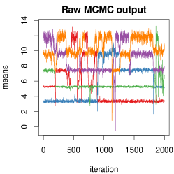
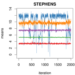
(a)	(b)	(c)
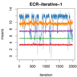
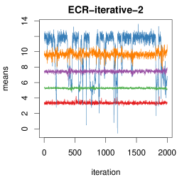
(d)	(e)	(f)
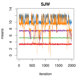
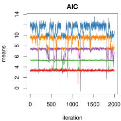
(g)	(h)	(i)

Figure 2: Fishery data. (a): Raw MCMC sample for $\mu_{k}$. (b), (c), (d), (e), (f), (g), (h), (i): Reordered MCMC sample by applying the permutations returned by label.switching function, according to methods: Stephens, PRA, ECR, ECR-iterative-1, ECR-iterative-2, SJW, AIC and Data-based, respectively.

The raw MCMC output for $\mu_{k}$, $k=1,\ldots,5$ is shown at Figure 2.(a) (every 5th iteration displayed). It is obvious that the label switching phenomenon has occurred. Note that a simple ordering constraint to the means is not able to successfully isolate one of the symmetric high posterior-density areas. Next, we will apply the function label.switching considering all the presented relabelling algorithms. In order to do this, we have to compute all the related information that is required as input for each method. At first, the MCMC output is converted into an $m\times K\times J$ array (mcmc.pars), where $J=3$ denotes the number of different parameter types for the normal mixture model: means (mcmc.pars[ , ,1]), variances (mcmc.pars[ , , 2]) and weights (mcmc.pars[ , ,3]). Finally, the generated allocation variables are stored to $m\times n$ array z: R> J <- 3 R> mcmc.pars <- array(data = NA, dim = c(m, K, J)) R> mcmc.pars[ , , 1] <- mcmc$results[-(1:burn),(n+K+1):(n+2*K)]R>mcmc.pars[,,2]<-mcmc$results[-(1:burn), (n+2*K+1):(n+3*K)] R> mcmc.pars[ , , 3] <- mcmc$results[-(1:burn),(n+1):(n+K)]R>z<-mcmc$results[-(1:burn), 1:n]

Stephens’ method as well as the second iterative version of ECR algorithm need the $m\times n\times K$ array of component membership probabilities $p_{ik}$, as defined in Equation 4, for each MCMC iteration. These probabilities are stored to array p as follows.

R> p <- array(data = NA, dim = c(m, n, K)) R> for (iter in 1:m) + for(i in 1:n) + kdist <- mcmc.pars[iter, , 3]*dnorm(x[i], mcmc.pars[iter, , 1], + sqrt(mcmc.pars[iter, , 2])) + skdist <- sum(kdist) + for(j in 1:K) + p[iter, i, j] = kdist[j]/skdist

Method sjw demands to provide as input a function that computes the complete log-likelihood of the classic mixture model, as defined by taking the logarithm of Equation 6. The next code accepts as input a dataset of univariate observations (x), an $n$-dimensional integer vector of allocations (z) and a $K\times J$ array of mixture parameters (means, variances, weights).

R> complete.normal.loglikelihood <- function(x, z, pars) + g <- dim(pars)[1] + n <- length(x) + logl <- rep(0, n) + logpi <- log(pars[ , 3]) + mean <- pars[ , 1] + sigma <- sqrt(pars[ , 2]) + logl <- logpi[z] + dnorm(x, mean = mean[z], sd = sigma[z], log = T) + return(sum(logl))

The function complete.normal.loglikelihood will be also used for the determination of an MCMC iteration that corresponds to a high density area. Next, the allocation and parameters of this iteration will be used as pivot by the functions ecr and pra, respectively. After evaluating the complete log-likelihood function for the 10000 MCMC iterations, we obtained that the maximum value corresponds to iteration mapindex = 4839.

We will also use an ordering constraint to the simulated means. Since this parameter type corresponds to mcmc.pars[ , , j] for j = 1, we should use constraint = 1. Now, we can apply the available algorithms using the following command. R> library("label.switching") R> set <- c("STEPHENS", "PRA", "ECR", "ECR-ITERATIVE-1", "ECR-ITERATIVE-2", + "SJW", "AIC", "DATA-BASED") R> ls <- label.switching(method = set, zpivot = z[mapindex, ], z = z, K = K, + prapivot = mcmc.pars[mapindex, , ], p = p, constraint = 1, + sjwinit = mapindex, complete = complete.normal.loglikelihood, + mcmc = mcmc.pars, data = x) R> ls$timings\text{Table 3Table 33Table 3DataKnmstephpraecrecr-1ecr-2sjwaicd-basedFish52561000056.93.53.417.813.4613.70.111.4Lamb42401000061.00.82.711.411.0598.50.18.5Multivariate 141001000025.70.82.510.76.0695.90.111.0Multivariate 2928015000431.3NA9.158.150.2NA0.161.13CPUtimesinsecondsperrelabellingmethod.Table 3CPUtimesinsecondsperrelabe}$