Long-run growth rate in a random multiplicative model

Abstract

We consider the long-run growth rate of the average value of a random multiplicative process $x_{i+1}=a_{i}x_{i}$ where the multipliers $a_{i}=1+\rho\exp(\sigma W_{i}-\frac{1}{2}\sigma^{2}t_{i})$ have Markovian dependence given by the exponential of a standard Brownian motion $W_{i}$. The average value $\langle x_{n}\rangle$ is given by the grand partition function of a one-dimensional lattice gas with two-body linear attractive interactions placed in a uniform field. We study the Lyapunov exponent $\lambda(\rho,\beta)=\lim_{n\to\infty}\frac{1}{n}\log\langle x_{n}\rangle$ at fixed $\beta=\frac{1}{2}\sigma^{2}t_{n}n$, and show that it is given by the equation of state of the lattice gas in thermodynamical equilibrium. The Lyapunov exponent has discontinuous first derivatives along a curve in the $(\rho,\beta)$ plane ending at a critical point $(\rho_{C},\beta_{C})$, which is related to a phase transition in the equivalent lattice gas. Using the equivalence of the lattice gas with a bosonic system, we obtain the exact solution for the equation of state in the thermodynamical limit $n\to\infty$.

I Introduction

Stochastic recursions of the form $x_{i+1}=a_{i}x_{i}+b_{i}$ with $x_{i}$ real-valued or matrix-valued quantities and $a_{i},b_{i}$ random variables have been widely considered as models of dynamics for various processes in physics, ecology, computer science, and economics Kadanoff ; Kesten ; LC ; Mitzenmacher ; Sornette . The most studied case corresponds to i.i.d. random coefficients $a_{i},b_{i}$ Kesten , but the case with state dependence (for example of Markovian type) has been also considered Cohen . Such processes can produce a wide variety of distributional properties for $x_{n}$ and under certain conditions on the coefficients $a_{i},b_{i}$ they can generate heavy-tailed distributions Kesten ; Goldie ; Mitzenmacher ; MSS ; Sornette . Alternative mechanisms for generating heavy tailed distributions with specific application to financial time series are discussed in MS ; Rachev .

We consider in this paper the discrete time random multiplicative process defined by

$$x_{i+1}=a_{i}x_{i}\,,\quad a_{i}=1+\rho e^{\sigma W_{i}-\frac{1}{2}\sigma^{2}t_{i}}$$ (1)

with $W_{i}=W(t_{i})$ the values of a standard Brownian motion starting at $W(0)=0$ and sampled at uniformly spaced times $t_{i}=i\tau$. The parameter $\rho$ is positive and bounded as $0\leq\rho<1$. This is a random multiplicative process with non-stationary multipliers $a_{i}$, which have Markovian dependence introduced through the dependence on the Brownian motion $W(t)$.

The model (1) can be used to describe the discrete time dynamics of a quantity which changes in each period by an amount which is proportional to its value at the beginning of the period. The random multiplier is positive and follows a geometric Brownian motion in discrete time. The simplest such variable is a bank account which accrues interest by simple compounding over each period $(t_{i},t_{i+1})$, assuming that the interest rate $L_{i,i+1}=L_{0}\exp(\sigma W_{i}-\frac{1}{2}\sigma^{2}t_{i})$ follows a geometric Brownian motion in discrete time. This corresponds to the Black, Derman, Toy model of stochastic interest rates in mathematical finance BDT . More generally, the model (1) could be used to describe multiplicative processes with Markovian dependence, such as for example of the type considered in Cohen in the context of population dynamics.

The random multipliers $a_{i}$ in Eq. (1) have the same average value $\langle a_{i}\rangle=1+\rho$. If the multipliers $a_{i}$ were independent random variables, one would expect the average of the process (1) to have a simple geometric growth as $\langle x_{n}\rangle=x_{0}(1+\rho)^{n}$. However, the successive multipliers $a_{i}$ are correlated through their dependence on the common Brownian motion $W_{i}$. Their covariance is

$$\mbox{cov}(a_{i},a_{j}) = \langle a_{i}a_{j}\rangle-\langle a_{i}\rangle\langle a_{j}\rangle$$

$$= \rho^{2}(e^{\sigma^{2}\mbox{min}(t_{i},t_{j})}-1)\,.$$

The average value $\langle x_{n}\rangle$ of the process (1) can be computed exactly, and displays a surprising explosive behavior for sufficiently large volatility $\sigma$ or sufficiently large time step $n$ RMP . This is very different from the naive expectation of a geometric growth obtained by assuming statistically independent multipliers, and is an effect due to the correlation between successive multipliers $a_{i}$. The same explosive behavior is noted also for the higher positive integer moments $\langle(x_{n})^{p}\rangle$. This implies that the probability distribution of the variable $x_{n}$ develops heavy tails under certain conditions.

The process (1) is somewhat similar to the Kesten process Kesten , which is defined by the stochastic recursion $x_{i+1}=a_{i}x_{i}+b_{i}$ with $a_{i},b_{i}$ i.i.d. random variables. For this case it has been shown Kesten ; Goldie that under certain conditions on the distributions of $a_{i},b_{i}$, the distribution of $x_{n}$ approaches a stationary form and has heavy tails (of regular variation). This class of models has been extended to accomodate also Markovian dependence for the $a_{i},b_{i}$ factors, see e.g. Cohen ; Roithershtein .

In this paper we consider the long-run asymptotics of the average value $\langle x_{n}\rangle$ of the process (1) in the limit $n\to\infty$ while keeping $\beta=\frac{1}{2}\sigma^{2}t_{n}n$ constant. This is described in terms of a Lyapunov exponent $\lambda(\rho,\beta)$, defined below in Eq. (3). We study the properties of the Lyapunov exponent and derive an exact solution for $\lambda(\rho,\beta)$ in terms of the equation of state of an equivalent one-dimensional lattice gas. The Lyapunov exponent is a continuous function of its arguments and has a discontinuous derivative along a curve in the $(\rho,\beta)$ plane ending at a critical point. The qualitative features of the exact solution are well reproduced in terms of an approximative mean-field theory with van der Waals equation of state.

II Lyapunov exponent and scaling

We study in this paper the long-run growth rate of the average value $\langle x_{n}\rangle$ of the process (1) as the number of time steps becomes very large $n\to\infty$. This can be described in terms of a Lyapunov exponent $\lambda$, defined as

$$\lambda=\lim_{n\to\infty}\frac{1}{n}\log\langle x_{n}\rangle\,.$$ (3)

A similar quantity and its properties were studied in the context of random multiplicative process with i.i.d. matrix-valued multipliers $a_{i}$ in Ruelle ; CN ; GG and for processes with Markovian dependence in Cohen .

For the study of the $n\to\infty$ limit it will prove helpful to make use of the equivalence between the process (1) and a lattice gas noted in RMP . We recall briefly the main points of this analogy. Consider a one-dimensional lattice gas with $n-1$ sites, and denote the occupation number of the site $i$ as $n_{i}=\{0,1\}$. The lattice gas particles interact by the Hamiltonian $H=\sum_{i<j}n_{i}n_{j}\varepsilon_{ij}$ where the interaction energy of two particles at sites $i,j$ is

$$\varepsilon_{ij}=\left\{\begin{array}[]{cc}-\frac{2}{n^{2}}\mbox{min}(i,j)&\,,i\neq j\\ +\infty&\,,i=j\end{array}\right.$$ (6)

Writing $-\min(i,j)=\frac{1}{2}|i-j|-\frac{1}{2}(i+j)$ the Hamiltonian can be put into the form

$$H=\sum_{i<j}n_{i}n_{j}\varphi_{ij}+\sum_{i}n_{i}\varphi_{i}$$ (7)

with translation invariant 2-body interaction $\varphi_{ij}=\frac{1}{n^{2}}|i-j|$ and single-site energies $\varphi_{i}=-\frac{1}{n^{2}}i$. The lattice gas particles attract each other with linear two-body interactions and are placed in a uniform strength field which drives them towards the right side of the lattice.

The precise relation of the random multiplicative process (1) to the one dimensional lattice gas with interaction (6) is given by the equality

$$\langle x_{n}\rangle=x_{0}{\cal Z}(\beta,\rho)\,,$$ (8)

between the average $\langle x_{n}\rangle$ and the grand partition function ${\cal Z}(\beta,\rho)$ of the lattice gas with fugacity $\rho$ and temperature $T=1/\beta$ with

$$\beta=\frac{1}{2}\sigma^{2}t_{n}n\,.$$ (9)

The grand partition function of the lattice gas is

$${\cal Z}(\beta,\rho)=\sum_{N=0}^{n-1}\rho^{N}Z_{N}(\beta)\,,$$ (10)

with $Z_{N}(\beta)$ the canonical partition function, given by a sum over all configurations with $N$ occupied sites

$$Z_{N}(\beta)=\sum_{\{n_{i}\},\sum_{i}n_{i}=N}e^{-\beta H}\,.$$ (11)

The relation (8) can be used to prove the following result: The Lyapunov exponent, defined as the limit

$$\lambda(\rho,T)\equiv\lim_{n\to\infty}\frac{1}{n}\log\langle x_{n}\rangle=\frac{1}{T}p(\rho,T)$$ (12)

exists and depends only on $\rho$ and $T=1/\beta$ with $\beta$ given by (9). Furthermore, $\lambda(\rho,T)$ is expressed as shown in terms of the pressure of the lattice gas $p(\rho,T)$.

This result follows from the existence of the thermodynamical limit for the lattice gas with interaction (6). A sufficient condition for the existence of this limit for a lattice gas with translation invariant 2-body interaction $\varphi_{ij}$ is the finiteness of the sum GMS

$$\sum_{j\neq i}|\varphi_{ij}|<\infty\,,$$ (13)

for any site $i$. One can easily check that this condition is indeed satisfied by the interaction (6). The factor $1/n^{2}$ was introduced in Eq. (6) motivated by this condition. Under this condition, the limit

$$\lim_{n\to\infty}\frac{1}{n}\log{\cal Z}(\beta,\rho)=\beta p(\rho,T)$$ (14)

exists and is a finite function of temperature $T$ and fugacity $\rho$ GMS . This function is related to the pressure of the lattice gas $p(\rho,T)$, which is given in terms of the thermodynamical potential as

$$\Omega=-T\log{\cal Z}=-np(\rho,T)\,.$$ (15)

The existence of the limit in (14) together with (8) implies the result (12). It is clear also from this derivation that the limit in (12) does not depend on the initial value $x_{0}$ of the random multiplicative process.

The result (12) shows that there is a close relationship between the long run asymptotics of the random multiplicative process (1) and the equilibrium thermodynamical properties of the lattice gas with interaction (6) in the thermodynamical limit $n\to\infty$. It also implies that the Lyapunov exponent $\lambda$ has a scaling property in the large $n$ limit, as it depends on $\sigma,\tau,n$ only through the combination $\beta=1/T$ defined in (9).

Numerical simulations show that the average $\langle x_{n}\rangle$ has an explosive behavior for sufficiently large $\sigma$ or $n$ RMP . We will show here that this phenomenon can be related to non-analyticity of the Lyapunov exponent $\lambda(\rho,T)$ in its arguments. In the next section we summarize the results of the numerical simulations, and in Sec. IV we present an analytical approximation based on a lower bound for the partition function of the lattice gas which corresponds to a van der Waals system, which reproduces the qualitative features of the numerical simulation. In Sec. V we present the exact solution for the Lyapunov exponent $\lambda(\rho,T)$ following from the equation of state of the lattice gas with interaction (6) in the thermodynamical limit.

III Numerical results

The integer positive moments $\langle(x_{n})^{p}\rangle$ of the random variable $x_{n}$ defined by the process (1) can be computed exactly, but numerically, using a recursion relation described in Appendix A of RMP . We use this method to compute the average value $\langle x_{n}\rangle$ and the finite $n$ approximation to the Lyapunov exponent $\lambda_{n}=\frac{1}{n}\log\langle x_{n}\rangle$.

We show in Figure 1 (upper panel) typical numerical results for $\lambda_{n}$ as function of temperature $T=1/\beta$ defined as in (9) for several values of $\rho$ between 0.005 and 0.125. The simulation has $n=200$ time steps of size $\tau=1$ and initial value $x_{0}=1$. The results of the simulation show that $\lambda_{n}$ is always positive and is a decreasing function of $T$, approaching a small but finite value as $T\to\infty$. The functional dependence is qualitatively different, depending on whether $\rho$ is below or above some critical value $\rho_{C}$. This suggests the following picture:

i) $\rho>\rho_{C}$. The Lyapunov exponent $\lambda(\rho,T)$ is a smooth decreasing function of temperature.

ii) $\rho<\rho_{C}$. The $T$ dependence of $\lambda(\rho,T)$ has a kink at a certain transition temperature $T_{\rm tr}(\rho)$, and its derivative with respect to $T$ is discontinuous at this point. As $T$ decreases below this value, $\lambda(\rho,T)$ increases very rapidly and explodes to infinity as $T\to 0$.

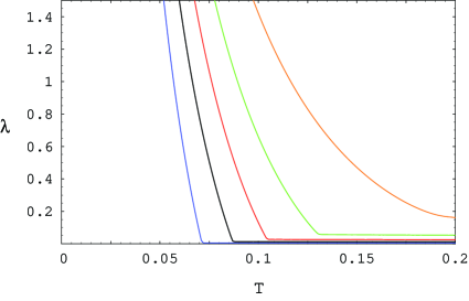
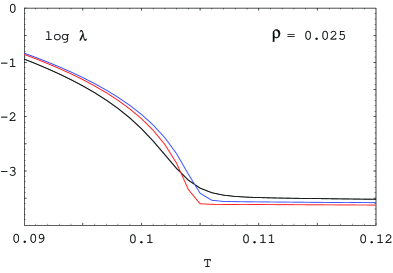
Figure 1: Above: The Lyapunov coefficient $\lambda_{n}=\frac{1}{n}\log\langle x_{n}\rangle$ as function of temperature $T$ for several values of the $\rho$ parameter $\rho=0.005,0.0125,0.025,0.05,0.125$ (from left to right). The simulation has $n=200$ time steps with $\tau=1$ and $x_{0}=1$. Below: the approach to the thermodynamical limit. Plots of $\log\lambda_{n}$ vs $T$ at $\rho=0.025$ for $n=40$ (black), $n=100$ (blue), $n=200$ (red).

The approach to the thermodynamical limit $n\to\infty$ is illustrated in Fig. 1 (lower panel) which shows $\log\lambda_{n}$ vs the temperature $T$ for $\rho=0.025$ as $n$ is increased: 40 (black), 100 (blue), 200 (red). These plots confirm the scaling property of the Lyapunov exponent, more precisely that $\lambda_{n}\to\lambda(\rho,T)$ approaches a function which depends only on $(\rho,T)$ in the $n\to\infty$ limit. The numerical results show that with $n=200$ the scaling property holds very well.

This picture can be used to understand the behavior of the expectation value $\langle x_{n}\rangle$ observed in numerical simulations as functions of the volatility $\sigma$, maturity $t_{n}$ and time step $\tau$ RMP . As the product $\frac{1}{2}\sigma^{2}t_{n}n$ (corresponding to the scaling variable $\beta$ defined in Eq. (9) which has the meaning of the inverse temperature) increases, the temperature of the equivalent lattice gas decreases. As long as the temperature $T$ is above the transition temperature $T_{\rm tr}(\rho)$, the lattice gas is in the gaseous phase and the pressure increases but remains small. The equivalent statement for the process (1) is that the average value $\langle x_{n}\rangle$ increases slowly. As soon as the temperature drops below the transition temperature, the lattice gas condenses into the liquid phase and the pressure increases very fast with the temperature, which translates into an explosive growth of the expectation $\langle x_{n}\rangle$. The approach to the $n\to\infty$ limit of the random multiplicative process (1) is discussed in more detail below in Sec. VI.

IV Van der Waals approximation

We present in this Section analytical approximations for the thermodynamical properties of the lattice gas with long-range interactions (6). These approximations are based on lower and upper bounds on the partition function of the lattice gas with the interaction (6)

$$\overline{\cal Z}(\beta,\rho)\geq{\cal Z}(\beta,\rho)\geq\underline{\cal Z}(\beta,\rho)\,.$$ (16)

These bounds are partition functions for lattice gases with uniform infinite range interactions. The lower bound has interaction RMP

$$\underline{\varepsilon}_{ij}=\left\{\begin{array}[]{cc}-\frac{2}{3n}&\,,i\neq j\\ +\infty&\,,i=j\end{array}\right.$$ (19)

The lower bound on the energy of a state with $N$ particles $E_{N}\geq E_{N}^{(0)}=\frac{1}{3n^{2}}N(N-1)(2N+2-3n)>-\frac{1}{n}$ gives an upper bound on the canonical partition function $Z_{N}(\beta)$ in terms of the partition function of a lattice gas with uniform interactions

$$\overline{\varepsilon}_{ij}=\left\{\begin{array}[]{cc}-\frac{2}{3n^{2}}(3n-2N-2)&\,,i\neq j\\ +\infty&\,,i=j\end{array}\right.$$ (22)

A weaker upper bound which has the advantage that it does not depend on the number of particles (similar to the lower bound (19)) is $\overline{\varepsilon}_{ij}=-\frac{2}{n},i\neq j$.

Each of these simpler systems is equivalent to a mean-field theory, as each particle feels the effect of the other particles as a constant interaction energy. Their thermodynamical properties are given by the van der Waals theory Kadanoff ; LP . The lower bound is saturated in the very large temperature limit $T\to\infty$ RMP , and is numerically more accurate for all temperatures. For this reason we will restrict ourselves to the predictions following from the lower bound.

The thermodynamical quantities of the approximative van der Waals system can be computed in closed form. The free energy corresponding to the lower bound (19) is $F(n,N,T)=nf(d,T)$ with $f(d,T)$ the free energy density, given by RMP ; LP

$$f(d,T)=CE[T(d\log d+(1-d)\log(1-d))-\frac{1}{3}d^{2}]$$ (23)

with $d=N/n$ the lattice gas density and $CE[f(d,T)]$ denotes the convex envelope of $f(d,T)$ with respect to $d$. The equation of state has van der Waals form

$$p=-T\log(1-d)-\frac{1}{3}d^{2}\,,$$ (24)

supplemented with the Maxwell construction, which replaces (24) with a constant pressure $p_{0}(T)$ in the region $d_{g}\leq d\leq d_{\ell}$ with

$$d_{g}(T)=\frac{1}{2}(1-\Delta)\,,\qquad d_{\ell}(T)=\frac{1}{2}(1+\Delta)$$ (25)

where $\Delta$ is the positive solution of the equation $\Delta=\tanh\Big{(}\frac{\Delta}{6T}\Big{)}$.

The fugacity $\rho$ is

$$\rho=\frac{d}{1-d}e^{-\frac{2d}{3T}}\,.$$ (26)

The inversion of this relation in order to find $d$ for given $(\rho,T)$ requires some care. For $T\geq T_{C}=1/6$ this equation has a unique solution for $d$. For $T<1/6$ it has three solutions. Denoting the smallest and largest solutions with $d_{1}(\rho,T)$ and $d_{2}(\rho,T)$, respectively, the lattice gas density is given by

$$d(\rho,T)=\left\{\begin{array}[]{cc}d_{2}(\rho,T)&\,,\rho>e^{-\frac{1}{3T}}\\ d_{1}(\rho,T)&\,,\rho<e^{-\frac{1}{3T}}\\ \end{array}\right.$$ (29)

At $\rho=e^{-\frac{1}{3T}}$ the gas and liquid phases can co-exist, and their densities are

$$d_{2}(e^{-\frac{1}{3T}},T)=d_{\ell}(T)\,,\qquad d_{1}(e^{-\frac{1}{3T}},T)=d_{g}(T)\,.$$ (30)

These results can be used to understand the qualitative behavior of the curves for the Lyapunov exponent $\lambda(\rho,T)$ in Fig. 1. In the van der Waals approximation this is given by

$$\lambda_{\rm vdW}=\left\{\begin{array}[]{cc}-\log(1-d)-\frac{d^{2}}{3T}\,,&d\not\in(d_{g}(T),d_{\ell}(T))\\ \frac{1}{T}p_{0}(T)\,,&d\in(d_{g}(T),d_{\ell}(T))\\ \end{array}\right.$$ (33)

with $d=d(\rho,T)$ given by Eq. (29), and $p_{0}(T)$ corresponds to the flat portion of the isothermal curves and is determined such that $\lambda_{\rm vdW}$ is a continuous function of $d$. The shape of the curves $\lambda_{\rm vdW}$ vs $d$ is shown in Fig. 2 (lower plot) and are essentially the well-known van der Waals isothermal curves.

The function $\lambda_{\rm vdW}(\rho,T)$ at fixed $\rho$ has a discontinuous derivative with respect to $T$ at the transition temperature

$$T_{\rm tr}^{\rm(vdW)}(\rho)=-\frac{1}{3\log\rho}\,,$$ (34)

provided that the fugacity is below the critical value $\rho<\rho_{C}=e^{-2}$. Alternatively, at fixed $T$ the transition occurs at the point $\rho=\exp(-\frac{1}{3T})$ where the solution for $d$ in (29) changes branches and switches between $d_{1}$ and $d_{2}$. At this point the pressure is a continuous function of $T$ but its derivative has a jump. The maximal value of $\rho$ for which the transition occurs corresponds to the critical point of the van der Waals system which has parameters

$$T_{C}=\frac{1}{6}\,,\quad d_{C}=\frac{1}{2}\,,\quad\rho_{C}=e^{-2}\,.$$ (35)

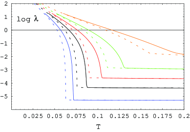
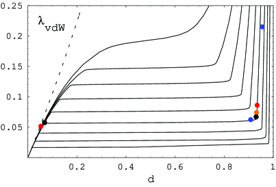
Figure 2: Above: Plots of $\log\lambda$ vs the temperature $T$ at fixed fugacity $\rho$. Solid curves: numerical solution for the lattice gas with interaction (6) with $n=200$ sites, dashed curves: the van der Waals approximation $\lambda_{\rm vdW}$ corresponding to the system (19). The colors correspond to the same values of the fugacity $\rho$ as in Fig. 1. Below: The Lyapunov exponent $\lambda_{\rm vdW}$ vs the lattice gas density $d$ at fixed temperature. The curves shown correspond to $T=0.08-0.15$ in steps of 0.01 and $T_{C}=1/6$ (from bottom to top). The colored dots are on the $\rho=0.05$ curve, see explanation in text. The dashed line shows the ideal gas approximation $\lambda=-\log(1-d)$.

These results are illustrated in Fig. 2. The upper plot shows $\log\lambda(\rho,T)$ as function of the temperature $T$ at fixed fugacity $\rho$. The solid lines correspond to the numerical simulation for the exact lattice gas with interaction (6) while the dashed curves correspond to the van der Waals approximation (33). Both these curves show a sharp transition at an intermediate transition temperature $T_{\rm tr}(\rho)$ which depends on the fugacity $\rho$.

In order to understand better the discontinuous behavior of the pressure $p(\rho,T)$ with respect to $T$ at fixed fugacity $\rho$ we show in the lower panel of Fig. 2 plots of $\lambda_{\rm vdW}$ vs the density of the lattice gas $d$ for several values of the temperature $T=0.08-0.15$ in steps of $0.01$ (from bottom to top). The top-most curve corresponds to $T=T_{C}=1/6$. The colored dots are on the curve of constant fugacity $\rho=0.05$ and correspond to increasing temperature. The points to the right of the horizontal portion correspond to $T=0.105,0.11,0.1105,0.1108,0.111$ and the points to the left correspond to $T=0.12,0.3$ (from top to bottom). The transition temperature for this fugacity is $T_{\rm tr}^{(vdW)}(0.05)=-1/(3\log 0.05)=0.1113$. As $T$ increases above the transition temperature, the density drops suddenly from the right side (liquid phase) to the left side of the flat portion of the isothermal curve (gas phase), and the lattice gas evaporates. As explained above, this jump is responsible for the discontinuity in the slope of the curve $p(\rho,T)$ vs $T$ at fixed $\rho$, occuring at the transition temperature $T_{\rm tr}(\rho)$.

Using the van der Waals picture we can obtain analytical expressions for the Lyapunov exponent $\lambda_{\rm vdW}(T,\rho)$ in the small- and large-temperature limits, which describe the right and left tails of the curves in Fig. 2 (upper plot).

In the large-temperature limit $T\to\infty$ the lattice gas is in the gas phase. From Eq. (33) the Lyapunov exponent becomes approximatively equal to $\lambda_{\rm vdW}\simeq-\log(1-d)$ in this limit. Inversion of Eq. (26) gives that the density approaches a constant value $d(\rho,T)=\frac{\rho}{1+\rho}+O(T^{-1})$. Substituting into (33) gives the large temperature limit of the the van der Waals approximation of the Lyapunov exponent

$$\lim_{T\to+\infty}\lambda_{\rm vdW}(\rho,T)=\log(1+\rho)\,.$$ (36)

The independence on temperature of this limiting value is due to the fact that $p/T$ approaches a universal function in the small density limit, which is just ideal gas behavior. This is seen as the overlap of all the isothermal curves in the low density region $d\ll 1$ in the lower panel of Fig. 2. All these curves approach the ideal gas equation of state $p/T=d$ which is shown as the dashed line.

The result (36) agrees with the $\sigma=0$ limiting behavior of the random multiplicative process (1) which is solved trivially as $x_{n}=x_{0}(1+\rho)^{n}$. This gives $\lambda|_{\sigma\to 0}=\log(1+\rho)$.

In the small-temperature limit $T\to 0$ the lattice gas is in the liquid phase. The density $d$ is close to 1, and is given by the approximative solution of (26)

$$\lim_{T\to 0}d(\rho,T)=1-\frac{1}{1+\rho e^{\frac{2}{3}\beta}}\,.$$ (37)

Susbtituting into the expression (33) we obtain the small-temperature asymptotics of the Lyapunov exponent

$$\lim_{T\to 0}\lambda_{\rm vdW}(\rho,T)=\log(1+\rho e^{\frac{2}{3}\beta})-\frac{1}{3}\beta\simeq\log\rho+\frac{1}{3T}\,.$$ (38)

This gives an explosive behavior of $\lambda_{\rm vdW}(\rho,T)$ as $T\to 0$ which reproduces the results of the numerical simulation shown in Fig. 2 (upper plot).

The relations (36) and (38) give the small- and large-temperature asymptotic behavior of the van der Waals approximation for the Lyapunov exponent of the random multiplicative process. As seen from Fig. 2 (upper plot), they reproduce reasonably well the main qualitative features of the curves obtained from the exact numerical simulation of the model.

V Exact solution in the thermodynamical limit

The thermodynamical properties of the lattice gas with interaction (6) can be found exactly in the thermodynamical limit $n,N\to\infty$ at fixed particle density $d=N/n$. We start by stating the solution.

Proposition 1.

The free energy density of the lattice gas with interaction (6) is given by the convex envelope with respect to $d$ of the function

$$f(d,T) = \frac{1}{3}d^{2}(2d-3)+\pi(d-1)$$

$$+ Td\int_{0}^{1}dy\log(1-e^{-\beta[d^{2}y(2-y)+\pi]})\,,$$

where the intensive quantity $\pi(d,T)$ is defined by the solution of the equation

$$\frac{1}{d}-1=\int_{0}^{1}\frac{dy}{e^{\beta[d^{2}y(2-y)+\pi]}-1}\,,$$ (40)

with $d=N/n$ the density of the lattice gas.

The thermodynamical pressure is

$$p(d,T) = -f(d,T)+d\partial_{d}f(d,T)$$

$$=\frac{1}{3}d^{2}(4d-3)+\pi+2d^{3}\int_{0}^{1}dy\frac{y(2-y)}{e^{\beta[d^{2}y(2-y)+\pi]}-1)}\,.$$

The Gibbs free energy density $g(d,T)$ defined as $G=E-TS+\pi n=ng(d,T)=n(f(d,T)+\pi)$, is given by

$$g(d,T) = \frac{1}{3}d^{2}(2d-3)+\pi d$$

$$+ Td\int_{0}^{1}dy\log(1-e^{-\beta[d^{2}y(2-y)+\pi]})\,.$$

The chemical potential $\mu=\partial_{d}f(d,T)$ is given by the change of the free energy density at fixed volume $n$ and temperature $T$ when adding one particle. The lattice gas fugacity is

$$\rho(d,T)=e^{\beta\mu}=\exp\Big{(}\frac{1}{T}\partial_{d}f(d,T)\Big{)}\,.$$ (43)

We will derive these results using the isobaric-isothermal ensemble. A good introduction to the isobaric-isothermal ensemble and its applications to lattice gases can be found in Appendix 4 of Hill Hill . The proof is based on the equivalence of the lattice gas with $n-1$ sites and $N$ particles with a boson system of $n-N-1$ bosons which can be placed onto $N+1$ known energy levels $\omega_{k},k=0,1,\cdots,N$. The isobaric-isothermal ensemble for the lattice gas will be shown to be equivalent with the grand canonical ensemble for the equivalent bosonic system.

We start by recalling the energy spectrum of the lattice gas with interaction (6). The energy of the lattice gas with interaction (6) and $N$ particles is given by (see Proposition 1 of RMP )

$$E_{N}=E_{N}^{(0)}+\sum_{k=0}^{N}y_{k}\omega_{k}$$ (44)

where $y_{k}=0,1,2,\cdots$ are the occupation numbers of the energy levels $\omega_{k}$ which are given by

$$\omega_{k}=\frac{2}{n^{2}}k(N-\frac{1}{2}(k+1))\,,\qquad k=0,1,\cdots,N\,.$$ (45)

The ground state energy is

$$E_{N}^{(0)}=\frac{1}{3n^{2}}N(N-1)(2N+2-3n)\,.$$ (46)

The occupation number $y_{k}$ of the $k-$th energy level has a geometrical interpretation as the number of the empty sites between the $(k-1)-$th and $k-$th particles on the lattice (ordered in increasing order $i_{1}<i_{2}<\cdots<i_{N}$). (For $k=0$ the variable $y_{0}$ has the meaning of the number of empty lattice sites to the left of the leftmost particle.) They satisfy the sum rule $\sum_{k=0}^{N}y_{k}=n-N-1$ which has a simple geometrical interpretation as the total number of the empty sites of the lattice gas. It is clear that the states and the energy of this system are exactly equivalent to those of a system of $n-N-1$ bosons which can be placed onto the $N+1$ energy levels $\omega_{k}$.

In the isothermal-isobaric ensemble one fixes the number of particles $N$ and the temperature $T$, while the lattice size $n$ (volume) is allowed to be variable, subject only to the constraint $n\geq N$. Furthermore, an intensive quantity $\pi$ is introduced, which is fixed and is usually identified with the pressure of the system. One defines the isothermal-isobaric partition function as

$$\Xi(\pi,T)=\sum_{m=N}^{\infty}Z_{N}(m)e^{-\beta\pi m}\,.$$ (47)

Here $Z_{N}(n)$ is the usual canonical partition function of the lattice gas with $n$ sites and $N$ particles. The Gibbs free energy $G$ and the free energy $F$ are determined as

$$G=F+\pi(d,T)n=-T\log\Xi(\pi,T)$$ (48)

where the intensive quantity $\pi(d,T)$ is determined from the equation for the average lattice size

$$n=-\partial_{\pi}\Xi(\pi,T)\,.$$ (49)

In order to be able to perform the sum over $m$ in (47) in closed form we replace $m\to n$ in the denominator of (6), where $n$ is a fixed value which will be set equal to the actual lattice size $n$. As a result the same replacement is made in the denominators of (45) and (46). We will identify in the intermediate steps $N/n=d$ with the density of the lattice gas. The replacement of the summation index $m$ with the average value of the lattice size $n$ is justified in the thermodynamical limit, when the fluctuations of the volume $m$ around its mean become vanishingly small. However, this replacement has the effect that the intensive quantity $\pi$ is not exactly equal to the pressure of the lattice gas.

Using the representation (44) we write the canonical partition function as

$$Z_{N}(m) = e^{-\beta E_{N}^{(0)}}\bar{Z}_{N}(m)$$

$$= \exp\Big{(}-\frac{\beta}{3n^{2}}N(N-1)(2N+2-3m)\Big{)}\bar{Z}_{N}(m)\,,$$

where we introduced $\bar{Z}_{N}(m)$ the partition function of a system with energy $\bar{E}_{N}=\sum_{k=0}^{N}y_{k}\omega_{k}$ and $\sum_{k=0}^{N}y_{k}=m-N-1$.

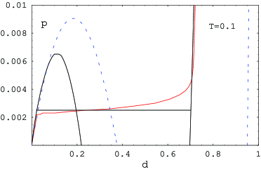
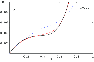
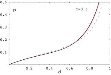
Figure 3: The exact isothermal curves $p(d,T)$ (black) of the lattice gas (6) obtained from Eq. (1). The horizontal black line in the upper plot was obtained by the Maxwell construction as described in Sec. V.2. The numerical solution on a lattice gas with $n=200$ sites is shown as the red curve. The van der Waals approximation of the isothermal curves $p_{\rm vdW}(d,T)$ given in Eq. (24) is shown as the dashed blue curves. The three plots correspond to $T=0.1,0.2,0.3$.

The sum over $m$ in (47) can be evaluated in closed form using the combinatorial identity

$$\sum_{m=N}^{\infty}\bar{Z}_{N}(m)e^{-\beta m\pi}=\frac{e^{-\beta N\pi}}{\Pi_{k=0}^{N}(1-e^{-\beta(\omega_{k}+\pi)})}\,.$$ (51)

This has a clear resemblance to the grand partition function of a system of non-interacting bosons which can be placed onto $N+1$ energy levels $\omega_{k}$, see e.g. bosongas . The intensive quantity $\pi$ is the analog of the (minus) chemical potential for the boson system.

The isothermal-isobaric partition function of the lattice gas is

$$\Xi(\pi,T)=e^{-\frac{2}{3}\beta d^{2}(N+1)}\frac{e^{-\beta N(\pi-d^{2})}}{\Pi_{k=0}^{N}(1-e^{-\beta(\omega_{k}+\pi-d^{2})})}$$ (52)

The Gibbs free energy is obtained as

$$G(\pi,T) = -T\log\Xi(\pi,T)$$

$$=\frac{2}{3}d^{2}(N+1)+N(\pi-d^{2})$$

$$+T\sum_{k=0}^{N}\log(1-e^{-\beta(\omega_{k}+\pi-d^{2})})\,.$$

In the $N\to\infty$ limit the sum can be replaced with an integral as

$$\sum_{k=0}^{N}\log(1-e^{-\beta(\omega_{k}+\pi-d^{2})})\simeq$$ (54)

$$N\int_{0}^{1}dy\log\Big{(}1-e^{-\beta(d^{2}y(2-y)+\pi-d^{2})}\Big{)}\,.$$

Collecting together all the terms we find the result for the free energy density

$$f(d,T) = \frac{G}{n}-\pi=\frac{2}{3}d^{3}+\pi(d-1)$$

$$+ Td\int_{0}^{1}dy\log\Big{(}1-e^{-\beta(d^{2}y(2-y)+\pi-d^{2})}\Big{)}\,.$$

The convex envelope of this function with respect to $d$ is understood. This reproduces the relation Eq. (1) upon replacing $\pi-d^{2}\to\pi$. Since $\pi$ is not an observable quantity we can redefine it by a shift $\pi-d^{2}\to\pi$, in order to simplify the form of the result. Alternatively, the result Eq. (1) can be directly obtained by replacing $m\to n$ also in the numerator of $E_{N}^{(0)}$ in Eq. (V).

The pressure is obtained as

$$p(d,T)=-f(d,T)+d\partial_{d}f(d,T)\,.$$ (56)

Substituting here $f(d,T)$ from Eq. (V) and replacing again $\pi-d^{2}\to\pi$ gives the result (1).

The intensive quantity $\pi$ is determined from the condition that the average lattice size is equal to its actual value $\langle m\rangle=n$. This is expressed as

$$n=-T\partial_{\pi}\log\Xi(\pi,T)=N+\sum_{k=0}^{N}\frac{1}{e^{\beta(\omega_{k}+\pi-d^{2})}-1}\,.$$ (57)

This has again a clear resemblance to the Bose-Einstein distribution, as it expresses the total number of bosons $n-N$ as a sum over the Bose-Einstein distribution for all energy levels $\omega_{k}$

$$n-N=\sum_{k=0}^{N}\frac{1}{e^{\beta(\omega_{k}+\pi-d^{2})}-1}\,.$$ (58)

Replacing the sum with an integral in the $N\to\infty$ limit gives

$$n-N=N\int_{0}^{1}dy\frac{1}{e^{\beta(d^{2}y(2-y)+\pi-d^{2})}-1}$$ (59)

which reproduces the equation (1) with the substitution $\pi-d^{2}\to\pi$. This completes the proof of Proposition 1

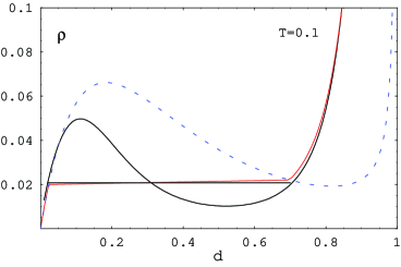
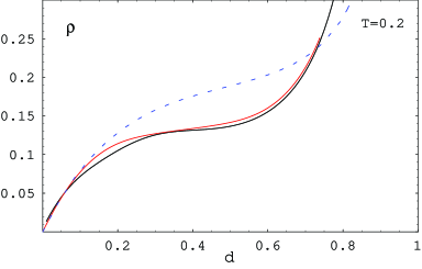
Figure 4: The exact fugacity $\rho(d,T)$ of the lattice gas (black curve) from Eq. (43). The horizontal black line in the upper plot was obtained by the Maxwell construction described in text. The numerical solution for $\rho(d,T)$ for a lattice gas with $n=200$ sites is shown as the red curve. The van der Waals approximation $\rho(d,T)$ given in Eq. (26) is shown as the dashed blue curves. The plots correspond to $T=0.1,0.2$.

V.1 Properties of the exact solution

We prove here a few properties of the exact solution presented in Proposition 1.

The equation

$$\frac{1}{d}-1=\int_{0}^{1}\frac{dy}{e^{\beta[d^{2}y(2-y)+\pi]}-1}\,.$$ (60)

has a unique solution $\pi(d,T)>0$ for any $0<d\leq 1$ and $T>0$. This implies that there is no analog of the Bose-Einstein condensation in the equivalent bosonic system. Furthermore, the solution $\pi(d,T)$ is bounded from below as

$$\pi(d,T)\geq\tilde{\pi}(d,T)=-T\log(1-d)-\frac{2}{3}d^{2}\,.$$ (61)

To prove this result, consider the integral

$$I(\pi)=\int_{0}^{1}\frac{dy}{e^{\beta[d^{2}y(2-y)+\pi]}-1}\,.$$ (62)

This is a monotonously decreasing function of $\pi$ for $\pi>0$, which approaches zero as $\pi\to\infty$ and diverges to $+\infty$ as $\pi\to 0$. This implies that the equation $1/d-1=I(\pi)$ has a unique positive solution for $\pi$ for any value of $d\in(0,1)$.

The function $I(\pi)$ is bounded from below as

$$I(\pi)\geq\tilde{I}(\pi)=\frac{1}{e^{\beta[\frac{2}{3}d^{2}+\pi]}-1}$$ (63)

This follows from the Jensen inequality, as $(e^{\beta[d^{2}y(2-y)+\pi]}-1)^{-1}$ is a convex function of $y$. As a result we have

$$\int_{0}^{1}\frac{dy}{e^{\beta[d^{2}y(2-y)+\pi]}-1}\geq\frac{1}{e^{\beta[\frac{2}{3}d^{2}+\pi]}-1}\,.$$ (64)

Using this into (1) gives the inequality (61).

Numerical simulation shows that the inequality (61) approaches saturation in the large temperature $T\to\infty$ limit.

Define the integral

$$J(x)\equiv\int_{0}^{1}dy\log\Big{(}1-e^{-\beta d^{2}y(2-y)+x}\Big{)}\,.$$ (65)

Numerical simulation shows that in the large temperature limit the integral (65) approaches the limiting value

$$\lim_{T\to\infty}J(\beta\pi)=\log d\,.$$ (66)

Substituting $\pi\to\tilde{\pi}$ and $J\to\log d$, the free energy density becomes

$$\lim_{T\to\infty}f(d,T)=TA(d)-\frac{1}{3}d^{2}$$ (67)

with $A(d)=d\log d+(1-d)\log(1-d)$. This coincides with the van der Waals result corresponding to the lower bound on the canonical partition function (19). This bound implies that the free energy density is bounded from above as

$$f(d,t)\leq TA(d)-\frac{1}{3}d^{2}\,.$$ (68)

The bound is saturated in the large temperature limit and gives the van der Waals equation of state of the lattice gas (6)

$$p_{\rm vdW}(d,T)=-T\log(1-d)-\frac{1}{3}d^{2}\,.$$ (69)

It is possible that the inequality (68) can be proved also analytically starting from the definition of $\pi(d,T)$ given by (1) but the author was unable to do so. However, the numerical solution confirms that this inequality is indeed satisfied in all cases considered.

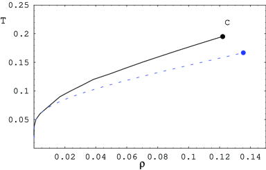
Figure 5: The phase co-existence curve $T_{\rm tr}(\rho)$ following from the exact solution of the model (black curve). This ends at the critical point $C$ with coordinates given in (71). The blue dashed curve shows the van der Waals approximation $T_{\rm tr}^{\rm(vdW)}(\rho)=-1/(3\log\rho)$.

V.2 Numerical results for the exact solution

We present in this section the numerical results for the thermodynamical quantities of the lattice gas following from the exact solution in the thermodynamical limit.

Fig. 3 shows numerical results for the isothermal curves $p=p(d,T)$ for several values of the temperature $T$ obtained by solving the equation (1). The curves $p(d,T)$ have a qualitative resemblance to the van der Waals isothermal curves. For sufficiently small temperature, below a critical temperature $T<T_{C}$, the pressure has two extremal points as function of $d$ (van der Waals loops), while for $T>T_{C}$ the pressure is a monotonously increasing function of $d$. The critical isothermal curve $T=T_{C}$ has an inflexion point where the second derivative vanishes $\partial_{d}^{2}p(d,T_{C})=0$.

The isothermal curves for $T<T_{C}$ must be supplemented by the Maxwell construction. This determines the flat portion of the pressure curve $p_{0}(T)$ and the gas, liquid densities $d_{g}(T),d_{\ell}(T)$ from the equal-area condition

$$\int_{d_{g}(T)}^{d_{\ell}(T)}\frac{dx}{x^{2}}(p(x,T)-p_{0}(T))=0\,.$$ (70)

The results for $d_{g}(T),d_{\ell}(T)$ can be used to find the fugacity $\rho_{0}(T)$ at which the two phases are in equilibrium at temperature $T$. The result is shown in Fig. 4, where we compare the exact result for $\rho(d,T)$ (black curves) against a numerical solution for a lattice gas with $n=200$ curves (red curves) and the van der Waals approximation (dashed blue curves).

The curve $\rho_{0}(T)$ defines the phase co-existence curve. This is shown in Fig. 5 as the black solid curve, together with its van der Waals approximation $T_{\rm tr}^{\rm(vdW)}(T)=-\frac{1}{3\log\rho}$ (blue dashed curve). It starts at origin and ends at the critical point $(\rho_{C},T_{C})$. The exact solution of the lattice gas given by the Proposition 1 gives the following approximative values for the critical parameters

$$T_{C}=0.195\,,d_{C}=0.36\,,\rho_{C}=0.122\,.$$ (71)

These are close to the critical parameters of the van der Waals approximative system $T_{C}=\frac{1}{6},d_{C}=\frac{1}{2},\rho_{C}=e^{-2}$.

VI Long-run and continuous time limits

We consider in this section the implications of the results for the Lyapunov exponent on the asymptotics of the average value $\langle x_{n}\rangle$ of the random multiplicative process (1) in the long-run and continuous time limits. The long-run asymptotics of the average has the general form

$$\lim_{n\to\infty}\langle x_{n}\rangle=ce^{\lambda(\rho,T)n}$$ (72)

with $c$ a constant independent of $n$ and $\lambda(\rho,T)$ depends on the two parameters of the equivalent lattice gas system: $\rho$ and $T=1/\beta$ with $\beta$ defined in (9).

VI.1 Long-run limit $n\to\infty$ at fixed time step $\tau$

Consider the behavior of $\langle x_{n}\rangle$ at fixed model parameters $\sigma,\rho,\tau$ as $n\to\infty$. This corresponds to the scaling

$$\rho=\mbox{fixed}$$ (73)

$$T=\frac{2}{\sigma^{2}\tau n^{2}}=\frac{c}{n^{2}}$$ (74)

As $n$ is increased, the temperature of the equivalent lattice gas decreases. The state of the system is described by a point which describes a linear trajectory in the $(\rho,T)$ plane, given by a vertical line ending at $T=0$, see Fig. 6.

We distinguish two possibilities for the behavior of the average $\langle x_{n}\rangle$ as $n\to\infty$. If $\rho<\rho_{C}$ (the orange line marked (I)), the trajectory intersects the phase co-existence curve, and the Lyapunov exponent $\lambda$ will have a discontinuous first derivative at the transition temperature $T_{\rm tr}(\rho)$ as shown in Fig. 1. At this point the average $\langle x_{n}\rangle$ has a fast explosive growth with $n$. If $\rho>\rho_{C}$ then the Lyapunov exponent has a smooth dependence on $T$, and the average $\langle x_{n}\rangle$ increases smoothly with $n$.

VI.2 Fixed maturity $t$ and volatility $\sigma$

We consider here the asymptotic behavior of $\langle x_{n}\rangle$ at fixed maturity $t_{n}=t$ and volatility $\sigma$ as the number of time steps is increased $n\to\infty$. The size of the time step decreases and approaches zero as $\tau=t/n\to 0$. We distinguish two possible cases:

i) fixed $\rho$. The equivalent lattice temperature scales with $n$ as

$$T=\frac{2}{\sigma^{2}tn}=\frac{c_{1}}{n}$$ (75)

and thus the system cools down as the number of time steps $n$ increases. The state of the system is described by a point which describes a linear trajectory in the $(\rho,T)$ plane, given by a vertical line ending at $T=0$, see Fig. 6. The behavior of the system is very similar to the case discussed above in Sec. VI.1.

If $\rho<\rho_{C}$ (the orange line marked (I)) then the Lyapunov exponent has a kink at the transition temperature $T_{\rm tr}(\rho)$ as shown in Fig. 1. If $\rho>\rho_{C}$ then the Lyapunov exponent has a smooth increase with $n$, without any discontinuous behavior.

ii) scaling $\rho=r\tau$ with fixed $r>0$. This corresponds to scaling both the temperature and fugacity to zero in a correlated manner such that their ratio stays constant

$$\beta=C_{1}n\,,\qquad\rho=C_{2}\frac{1}{n}\,,\mbox{ with }\beta\rho=\frac{1}{2}\sigma^{2}t^{2}r\,.$$ (76)

The state of the system is described by a trajectory in the $(\rho,T)$ plane which is a straight line joining the origin with the point $(rt,2/(\sigma^{2}t))$. The origin corresponds to the continuous time limit $n\to\infty$.

The qualitative behavior of the Lyapunov exponent as $n$ is taken to be very large is different depending on whether this line intersects the phase co-existence curve or not. These two cases are illustrated in Fig. 6 by the two dashed curves marked as (II) and (III). For the case (II) the Lyapunov exponent has a discontinuous derivative at the value of $n$ which corresponds to the intersection with the phase co-existence curve, while in case (III) the Lyapunov exponent has a smooth dependence and $\langle x_{n}\rangle$ increases smoothly as $n$ is increased.

VI.3 Continuous time limit

The $n\to\infty$ limiting form of the probability distribution function of $x_{n}$ for case ii) of Sec. VI.2 can be found in closed form. With the scaling $\rho=r\tau$, the random multiplicative process (1) approaches in the continuous time limit $\tau\to 0$ the diffusion defined by the stochastic differential equation

$$dx(t)=re^{\sigma W(t)-\frac{1}{2}\sigma^{2}t}x(t)dt\,.$$ (77)

Conversely, the random multiplicative process (1) can be regarded as an Euler discretization in time of the continuous time process (77).

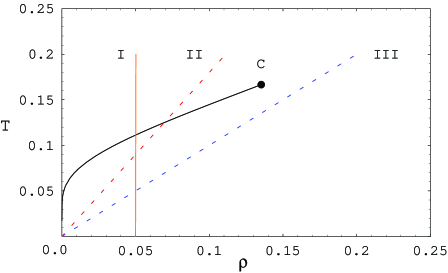
Figure 6: Paths in the plane $(\rho,T)$ corresponding to the different approaches to the $n\to\infty$ limit discussed in Sec V. The black solid curve shows the phase co-existence curve of Fig. 5, and ends at the critical point $C$. i) orange curve (I): fixed time step $\tau$, increasing time. ii) dashed blue and red curves (II), (III): fixed maturity $t_{n}$ and volatility, decreasing time step with scaling $\rho=r\tau$.

The solution of (77) is given by the exponential of the time integral of the geometric Brownian motion

$$x(t)=x(0)\exp\Big{(}r\int_{0}^{t}dse^{\sigma W(s)-\frac{1}{2}\sigma^{2}s}\Big{)}\,.$$ (78)

The distributional properties of this quantity are well studied in mathematical finance, see Dufresne0 ; Dufresne ; Yor ; Yor1 and references cited. We summarize here the main results.

Denote $\Phi(z,t)=\mathbb{P}(A(t)\in(z,z+dz))$ the probability distribution function of the time integral of the geometric Brownian motion

$$A(t)=\int_{0}^{t}dse^{\sigma W(s)-\frac{1}{2}\sigma^{2}s}\,.$$ (79)

This distribution approaches simple limits in the very small/large time limits respectively Dufresne2004 ; Dufresne . In the small time limit it approaches a normal distribution with mean $t$ and variance $\frac{1}{3}\sigma^{2}t$ Dufresne2004 , while in the infinite time limit it approaches a stationary distribution given by the inverse Gamma distribution Dufresne0 ; Dufresne

$$\lim_{t\to\infty}\Phi(z,t)=\frac{2}{\sigma^{2}z^{2}}e^{-\frac{2}{\sigma^{2}z}}\,.$$ (80)

This is derived as the stationary solution of the Fokker-Planck equation for the process $dX(t)=\sigma X(t)dW(t)+dt$ with $X(0)=0$. It was shown Dufresne0 that for any $t>0$, $X(t)$ has the same probability distribution as $A(t)$. For intermediate values of $t$, analytical expressions are also available, although they are rather involved, see Yor ; Yor1 and the references in these papers. The process leading to the distribution (80) is a particular case of a class of Markov processes which admit stationary solutions and were studied in Wong and Biro ; Bormetti .

The probability distribution $\Psi(y,t)$ of $y=x(t)/x(0)$ of the continuous time process has support $y:(1,\infty)$. In the very large time limit it approaches the stationary distribution

$$\lim_{t\to\infty}\Psi(y,t)=\frac{2r}{\sigma^{2}y\log^{2}y}e^{-\frac{2r}{\sigma^{2}\log y}}\,.$$ (81)

This gives the asymptotic $t\to\infty$ probability distribution of the random multiplicative process (1) in the continuous time limit under the scaling $\rho=r\tau$. This distribution has a power-like tail $\sim O(1/y)$, up to the slower varying logarithmic and exponential factors.

The expectation $\langle x(t)\rangle$ of the solution of the continuous time diffusion (78) is infinite under both $t\to 0$ and $t\to\infty$ limiting distributions. By the small time normal approximation for $A(t)$ Dufresne2004 , the variable $x(t)$ is approximatively log-normal in this limit

$$x(t)\simeq x(0)\exp(rte^{\sigma\sqrt{t/3}X-\frac{1}{6}\sigma^{2}t})\,,\quad t\to 0$$ (82)

where $X$ is a Gaussian random variable with mean zero and variance 1. The expectation of this random variable diverges, for arbitrarily small time. A similar divergence occurs for the $t\to+\infty$ limiting distribution (81). By the same argument, all positive integer moments of $x(t)$ are infinite.

VII Summary and discussion

We considered in this paper the long-run growth rate of the average value $\langle x_{n}\rangle$ of a discrete time random multiplicative process (1) driven by the exponential of a Brownian motion. The study of the $n\to\infty$ limit is considerably aided by the equivalence of this average value with the partition function of a one-dimensional lattice gas with $n$ sites and attractive interaction RMP . The $n\to\infty$ limit corresponds to the thermodynamical limit of the lattice gas, and can be studied using classical statistical mechanics methods.

The main results of the study can be summarized by the following properties of the Lyapunov exponent $\lambda$:

i) the Lyapunov exponent has a scaling property in the $n\to\infty$ limit. In this limit it approaches a function $\lambda(\rho,T)$, with $T=1/\beta$ where $\beta=\frac{1}{2}\sigma^{2}t_{n}n$ is a combination of the parameters of the process (1), which plays the role of the inverse temperature in the equivalent lattice gas. The Lyapunov exponent is related to the lattice gas pressure $p$ as $\lambda=1/Tp$.

ii) the functional dependence of $\lambda(\rho,T)$ for $\rho<\rho_{C}$ displays non-analyticity typical of a first-order phase transition. The Lyapunov exponent $\lambda(\rho,T)$ is a continuous function of $T$ at fixed $\rho$, but its derivative $\partial_{T}\lambda(\rho,T)$ is discontinuous at a transition point $T_{\rm tr}(\rho)$ provided that $\rho<\rho_{C}$. This behavior is related to a phase transition in the equivalent lattice gas. The qualitative features of this transition are reproduced to a good approximation in terms of a mean-field theory and van der Waals equation of state Kadanoff .

The results of this paper can be extended to the Lyapunov exponents associated with the higher positive moments of the state variable $\langle(x_{n})^{p}\rangle$ with $p\geq 2$. The numerical study in RMP showed that these moments have explosive behavior at certain values of the model parameters, similar to that observed for the average value. The analogy with the lattice gas can be extended also to these moments, which leads to the same scaling property as noted for the first moment in the $n\to\infty$ limit.

The model (1) can be generalized by replacing the standard Brownian motion $W_{i}$ with an arbitrary Gaussian stochastic process $Z_{i}$ sampled on a set of equidistant times $t_{i}$. The equivalence relation with a one-dimensional lattice gas (8) can be extended to such models by replacing the two-body interaction energy in Eq. (6) with $\varepsilon_{ij}=-\frac{1}{n^{2}}\mbox{cov}(Z_{i},Z_{j})$. The condition for the existence of the Lyapunov exponent is the same as the condition for the existence of the thermodynamical limit in the equivalent lattice gas. This requires that the covariance $\mbox{cov}(Z_{i},Z_{j})$ falls off sufficiently fast with $|i-j|$ such that the sum in (13) converges for any $i$ GMS . However, in order for a phase transition to be present, the covariance function $\mbox{cov}(Z_{i},Z_{j})$ cannot fall off too fast, and the interactions of the equivalent lattice gas must be sufficiently long-ranged Dyson . Sufficient conditions for the presence of a phase transition in a one-dimensional lattice gas are given in Dyson .

Assuming translation invariant interactions, the convergence of the sum $\sum_{j}|i-j|\varepsilon_{ij}$ has been shown to imply the absence of a phase transition RuelleLG ; GMR . In particular, this implies that taking $X(t)$ to be a stationary Ornstein-Uhlenbeck process for which the covariance decreases exponentially $\mbox{cov}(X(t)X(s))=\frac{\sigma^{2}}{2\gamma}e^{-\gamma|s-t|}$ does not produce a phase transition unless the mean-reversion parameter $\gamma$ is scaled in an appropriate way to zero, by taking the Kac limit KUH . Numerical simulations of such a model in RMP showed that the average $\langle x_{n}\rangle$ has a very rapid explosion with $\sigma$ at a certain point. According to the above argument this effect is expected to be smoothed out in the $n\to\infty$ limit such that the growth rate of $\langle x_{n}\rangle$ is an analytical function of the model parameters, and no phase transition is present in the analog lattice gas.

VIII Note added.

After the publication of this paper, an alternative exact result for the Lyapunov exponent $\lambda(\rho,\beta)$ has been obtained using large deviations theory in LDP . The treatment in LDP corresponds to working in the grand canonical ensemble. Although the numerical results obtained from the two solutions agree, their equivalence is not immediately apparent. We show here the equivalence of the two results.

VIII.1 Isobaric-isothermal ensemble

We summarize here the solution for the Lyapunov exponent obtained in the present paper, in a form appropriate for relating it to the grand canonical ensemble, at given fugacity $\rho$ and temperature $T$.

The Lyapunov exponent is

$$\lambda(\rho,\beta)=\beta p(d,T)$$ (83)

where $p(d,T)$ is given by equation (31) of the present paper which we repeat here for convenience

$$p(d,T)=\frac{1}{3}d^{2}(4d-3)+\pi+2d^{3}\int_{0}^{1}\frac{y(2-y)dy}{e^{\beta[d^{2}y(2-y)+\pi]}-1}\,.$$ (84)

In this equation $\pi(d,T)$ is given by the solution of the equation (29):

$$\frac{1}{d}-1=\int_{0}^{1}\frac{dy}{e^{\beta[d^{2}y(2-y)+\pi]}-1}\,.$$ (85)

The parameter $d$ is obtained from $(\rho,T)$ as the solution of equation (33)

$$\rho=e^{\beta\partial_{d}f(d,T)}$$ (86)

VIII.2 Grand canonical ensemble

In the grand canonical ensemble the Lyapunov exponent is given by LDP

$$\lambda(\rho,\beta)=\mbox{sup}_{d\in(0,1)}\Lambda(d)$$ (87)

where $\Lambda(d)$ is the function (see equation (90) of LDP )

$$\Lambda(d)=\beta d^{2}+\log(1+\rho)$$ (88)

$$-2\beta(1+\rho)d^{3}\int_{0}^{1}\frac{y^{2}dy}{1+\rho-e^{\beta d^{2}(y^{2}-1)}}\,.$$

The optimizer $d$ is given by the solution of the equation

$$\frac{1}{d}=(1+\rho)\int_{0}^{1}\frac{dy}{1+\rho-e^{\beta d^{2}(y^{2}-1)}}\,.$$ (89)

This can be put into an equivalent form by subtracting 1 from both sides

$$\frac{1}{d}-1=\int_{0}^{1}\frac{dy}{(1+\rho)e^{\beta d^{2}(1-y^{2})}-1}\,.$$ (90)

VIII.3 Relating the isothermal-isobaric and grand canonical ensembles

Proposition 2.

The intensive parameter $\pi$ in the isothermal-isobaric ensemble is related to the fugacity $\rho$ as

$$e^{\beta\pi}=1+\rho\,,\quad\mbox{ or equivalently, }\pi=T\log(1+\rho)\,.$$ (91)

Proof.

Make the change of integration variable $x=1-y$ in equation (85). This becomes

$$\frac{1}{d}-1=\int_{0}^{1}\frac{dx}{e^{\beta\pi}e^{\beta d^{2}(1-x^{2})}-1}$$ (92)

which is identical with (90) provided one identifies $e^{\beta\pi}=1+\rho$. ∎

Next we show that the thermodynamical pressure in the isobaric-isothermal ensemble (84) coincides with the grand canonical ensemble result (88).

Substitute the result (91) for $\pi$ into (84). Changing the integration variable as $y=1-x$ gives

$$p = \frac{1}{3}d^{2}(4d-3)+\pi+2d^{3}\int_{0}^{1}\frac{y(2-y)dy}{e^{\beta[d^{2}y(2-y)+\pi]}-1}$$

$$= \frac{1}{3}d^{2}(4d-3)+T\log(1+\rho)$$

$$+2d^{3}\int_{0}^{1}\frac{(1-x^{2})dx}{(1+\rho)e^{\beta d^{2}(1-x^{2})}-1}$$

The integral can be expressed using (90) as

$$\int_{0}^{1}\frac{(1-x^{2})dx}{(1+\rho)e^{\beta d^{2}(1-x^{2})}-1}=$$ (94)

$$\quad\frac{1}{d}-1-\int_{0}^{1}\frac{x^{2}dx}{(1+\rho)e^{\beta d^{2}(1-x^{2})}-1}\,.$$

This integral can be written further as

$$\int_{0}^{1}\frac{x^{2}dx}{(1+\rho)e^{\beta d^{2}(1-x^{2})}-1}=$$ (95)

$$\quad\int_{0}^{1}dxx^{2}\Big{(}\frac{1+\rho}{1+\rho-e^{\beta d^{2}(x^{2}-1)}}-1\Big{)}$$

$$\quad=(1+\rho)\int_{0}^{1}\frac{x^{2}dx}{1+\rho-e^{\beta d^{2}(x^{2}-1)}}-\frac{1}{3}$$

Substituting into (VIII.3) we get

$$p = d^{2}+T\log(1+\rho)$$

$$-2d^{3}(1+\rho)\int_{0}^{1}\frac{x^{2}dx}{1+\rho-e^{\beta d^{2}(x^{2}-1)}}$$

We see that $\beta p$ reproduces precisely the Lyapunov exponent obtained in the grand canonical ensemble, see Eqs. (87) and (88) above.

- (1) L. P. Kadanoff, Statistical physics: Statics, dynamics and renormalization, World Scientific, World Scientific Publishing, 2000.
- (2) H. Kesten, Random difference equations and renewal theory for products of random matrices, Acta Math. 131, 207 (1973).
- (3) R. C. Lewontin and D. Cohen, On population growth in a randomly varying environment, PNAS 62 (4), 1056 (1969).
- (4) D. Sornette, Critical phenomena in natural sciences: Chaos, fractals, self-organization and disorder: Concepts and Tools, Springer Series in Synergetics, 2006.
- (5) M. Mitzenmacher, A brief history of generative models for power law and log-normal distributions, Internet Mathematics 1, 226-251 (2004).
- (6) Y. Malevergne, A. Saichev and D. Sornette, Theory of Zipf’s law and beyond, Lecture Notes in Economics and Mathematical Systems, v. 632, Springer, 2009, [arXiv:q-fin/0808.1828.
- (7) C. M. Goldie, Implicit renewal theory and tails of solutions of random equations, Ann. Appl. Prob. 1, 126 (1991).
- (8) R. N. Mantegna and H. E. Stanley, Introduction to econophysics: Correlations and complexity in finance, Cambridge University Press, 1999.
- (9) S. T. Rachev (Ed.), Handbook of heavy tailed distributions in finance, v.1: Handbooks in finance, North Holland, New York, 2003.
- (10) D. Ruelle, Analyticity properties of the characteristic exponents of random matrix products, Adv. Math. 32 68-80 (1979).
- (11) J. E. Cohen, Long-run growth rates of discrete multiplicative processes in Markovian environments, J. Math. Analysis and Applications, 69, 243 (1979).
- (12) A. Roithershtein, One-dimensional linear recursions with Markov-dependent coefficients, Ann. Appl. Prob. 17, 572 (2007).
- (13) J. E. Cohen and C. M. Newman, The stability of large random matrices and their products, The Annals of probability 12, 283-310 (1984).
- (14) G. Gallavotti, Random matrices and Lyapunov coefficients regularity, arXiv:1311.5129 [nlin.CD]
- (15) D. Pirjol, Emergence of heavy-tailed distributions in a random multiplicative model driven by a stochastic Gaussian process, J. Stat. Phys. 154, 781-806 (2014).
- (16) D. Pirjol and L. Zhu, On the growth rate of a linear random recursion with Markovian dependence, Journal of Statistical Physics 160(5), 1354-1388 (2015)
- (17) F. Black, E. Derman and W. Toy, A one-factor model of interest rates and its application to treasury bond options, Fin. Anal. Journal 24-32 (1990).
- (18) G. Gallavotti and S. Miracle-Sole, Statistical mechanics of lattice systems, Comm. Math. Phys. 5, 317 (1967).
- (19) D. Ruelle, Statistical mechanics of a one-dimensional lattice gas, Comm. Math. Phys. 9, 267-346 (1968).
- (20) J. L. Lebowitz and O. Penrose, Rigorous treatment of the van der Waals-Maxwell theory of the liquid-vapor transition, J. Math. Phys. 7, 98 (1966).
- (21) T. L. Hill, Statistical mechanics. Principles and Selected Applications, Dover, 1987.
- (22) E. H. Lieb, R. Seiringer, J. P. Solovej and J. Yngvason, The quantum-mechanical many body problem: the Bose gas, arXiv:math-ph/0405004.
- (23) D. Dufresne, Weak convergence of random growth processes with applications to insurance, Insurance: Mathematics and Economics 8, 187-201 (1989).
- (24) D. Dufresne, The distribution of a perpetuity, with application to risk theory and pension funding, Scand. Actuarial J. 39-79 (1990).
- (25) D. Dufresne, The log-normal approximation in financial and other computations. Advances in Applied Probability 36(3), 747-773 (2004)
- (26) E. Wong, The construction of a class of stationary Markoff processes, in R. Bellman Ed. Stochastic Processes in Mathematical Physics and Engineering, 1964, 264-276.
- (27) C. Donati-Martin, R. Ghomrasni and M. Yor, On certain Markov processes attached to exponential functionals of Brownian motion: Applications to Asian options, Rev. Mat.Iberoamericana 17(1), 179-193 (2001).
- (28) A. Comtet, C. Monthus and M. Yor, Exponential functionals of Brownian motion and disordered systems, J. Appl. Prob. 35(2), 255-271 (1998).
- (29) T. S. Biro and A. Jakovác, Power-law tails from multiplicative noise, Phys. Rev. Lett. 94, 132302 (2005), [hep-ph/0405202].
- (30) G. Bormetti and D. Delpini, Exact moment scaling from multiplicative noise, Phys. Rev. E 81, 032102 (2010), arXiv:cond-mat/0911.5662.
- (31) F. Dyson, Existence of a phase transition in a one-dimensional Ising ferromagnet, Comm. Math. Phys. 12, 91 (1969).
- (32) G. Gallavotti, S. Miracle-Sole and D. Ruelle, Absence of phase transitions in one-dimensional systems with hard cores, Phys. Lett. 26A, 350-351 (1968).
- (33) M. Kac, G. E. Uhlenbeck and P. C. Hemmer, On the van der Waals theory of the vapor-liquid equilibrium: I. Discussion of a one-dimensional model, J. Math. Phys. 4, 216(1963).