The waveguide eigenvalue problem and the tensor infinite Arnoldi method

Abstract

We present a new computational approach for a class of large-scale nonlinear eigenvalue problems (NEPs) that are nonlinear in the eigenvalue. The contribution of this paper is two-fold. We derive a new iterative algorithm for NEPs, the tensor infinite Arnoldi method (TIAR), which is applicable to a general class of NEPs, and we show how to specialize the algorithm to a specific NEP: the waveguide eigenvalue problem. The waveguide eigenvalue problem arises from a finite-element discretization of a partial differential equation (PDE) used in the study waves propagating in a periodic medium. The algorithm is successfully applied to accurately solve benchmark problems as well as complicated waveguides. We study the complexity of the specialized algorithm with respect to the number of iterations $m$ and the size of the problem $n$, both from a theoretical perspective and in practice. For the waveguide eigenvalue problem, we establish that the computationally dominating part of the algorithm has complexity $\mathcal{O}(nm^{2}+\sqrt{n}m^{3})$. Hence, the asymptotic complexity of TIAR applied to the waveguide eigenvalue problem, for $n\rightarrow\infty$, is the same as for Arnoldi’s method for standard eigenvalue problems.

1 Introduction

Consider the propagation of waves in a periodic medium, which are governed by the Helmholtz equation

(1) $$\Delta v(x,z)+\omega^{2}\eta(x,z)^{2}v(x,z)=0,\qquad(x,z)\in\mathbb{R}^{2},$$

where $\eta\in L^{\infty}(\mathbb{R}^{2})$ is called the index of refraction and $\omega$ the temporal frequency. When (1) models an electromagnetic wave, the solution $v$ typically represents the $y$-component of the electric or the magnetic field. The (spatially dependent) wavenumber is $\kappa(x,z):=\omega\eta(x,z)$ and we assume that the material is periodic in the $z$-direction and without loss of generality the period is assumed to be 1, i.e., $\eta(x,z+1)=\eta(x,z)$. The index of refraction is assumed to be constant for sufficiently large $|x|$, such that $\kappa(x,z)=\kappa_{-}$ when $x<x_{-}$, $\kappa(x,z)=\kappa_{+}$ when $x>x_{+}$. In this paper we assume the wavenumber to be piecewise constant. Figure 1 shows an example of the setup.

Bloch solutions to (1) are those solutions that can be factorized as a product of a $z$-periodic function and $e^{\gamma z}$, i.e.,

(2) $$v(x,z)=\hat{v}(x,z)e^{\gamma z},\qquad\hat{v}(x,z+1)=\hat{v}(x,z).$$

The constant $\gamma\in\mathbb{C}$ is called the Floquet multiplier and without loss of generality, it is assumed that $\operatorname{Im}\gamma\in(-2\pi,0]$. We interpret (1) in a weak sense. We are only interested in Bloch solutions that decay in magnitude as $|x|\rightarrow\infty$ and we require that $\hat{v}$, restricted to $S:=\mathbb{R}\times(0,1)$, belongs to the Sobolev space $H^{1}(S)$. Moreover, we assume that any Bloch solution has a representative in $C^{1}(S)$. These solutions are in general not in $C^{2}(S)$ since $\kappa$ is discontinuous.

Figure 1: Illustration of a waveguide defined on $\mathbb{R}^{2}$. The wavenumber $\kappa(x,z)$ is constant in the three regions separated by the thick lines.

In this contex, Bloch solutions are also called guided modes of (1). If $\gamma$ is purely imaginary, the mode is called propagating; if $|\operatorname{Re}\gamma|$ is small it is called leaky. Both mode types are of great interest in various settings [14, 26, 30, 28, 2]. We present a procedure to compute leaky modes, with $\operatorname{Re}\gamma<0$ and $\operatorname{Im}\gamma\in(-2\pi,0)$. This specific setup has been studied, e.g., in [31].

To compute the guided modes one can either fix $\omega$ and find $\gamma$, or, conversely, fix $\gamma$ and find $\omega$. Both formulations lead to a PDE eigenvalue problem set on the unbounded domain $S$. When $\gamma$ is held fix, the eigenvalue problem is linear and if $\omega$ is held fix, it is nonlinear (quadratic) in $\gamma$. In this paper we fix $\omega$, and the substitution of (2) into (1) leads to the following problem. Find $(\gamma,\hat{v})\in\mathbb{C}\times H^{1}(S)$ such that

(3a) $$\;\;\;\;\;\;\;\;\Delta\hat{v}(x,z) + 2\gamma\hat{v}_{z}(x,z)+(\gamma^{2}+\kappa(x,z)^{2})\hat{v}(x,z)=0,\;\;(x,z)\in S,$$

(3b) $$\hat{v}(x,0) = \hat{v}(x,1),\;\;\textrm{}x\in\mathbb{R},$$

(3c) $$\hat{v}_{z}(x,0) = \hat{v}_{z}(x,1),\;\textrm{}x\in\mathbb{R}.$$

The problem (3), which in this paper is referred to as the waveguide eigenvalue problem, is defined on an unbounded domain. We use a well-known technique to reduce the problem on a unbounded domain to a problem on a bounded domain. We impose artificial (absorbing) boundary conditions, in particular so-called Dirichlet-to-Neumann (DtN) maps. See [16, 6] for literature on artificial boundary conditions.

The DtN-reformulation and a finite-element discretization, with rectangular elements generated by a uniform grid with $n_{x}$ and $n_{z}$ grid points in $x$ and $z$-direction correspondingly, is presented in section 2. A similar DtN-discretization has been applied to the waveguide eigenvalue problem in the literature [31]. In relation to [31], we need further equivalence results for the DtN-operator and use a different type of discretization, which allows easier integration with our new iterative method. Due to the fact that the DtN-maps depend on $\gamma$, the discretization leads to a nonlinear eigenvalue problem (NEP) of the following type. Find $(\gamma,w)\in\mathbb{C}\times\mathbb{C}^{n}\backslash\{0\}$ such that

(4) $$M(\gamma)w=0,$$

where

(5) $$M(\gamma):=\begin{bmatrix}Q(\gamma)&C_{1}(\gamma)\\ C_{2}^{T}&P(\gamma)\end{bmatrix}\in\mathbb{C}^{n\times n},$$

and $n=n_{x}n_{z}+2n_{z}$. The matrices $Q(\gamma)\in\mathbb{C}^{n_{x}n_{z}\times n_{x}n_{z}}$ and $C_{1}(\gamma)\in\mathbb{C}^{n_{x}n_{z}\times 2n_{z}}$ are a quadratic polynomials respect $\gamma$, $Q(\gamma)=A_{0}+A_{1}\gamma+A_{2}\gamma^{2}$, $C_{1}(\gamma)=C_{1,0}+C_{1,1}\gamma+C_{1,2}\gamma^{2}$, where $A_{i},C_{1,i}$ and $C_{2}^{T}$ are large and sparse. The matrix $P(\gamma)$ has the structure

(6) $$P(\gamma)=\begin{bmatrix}R\Lambda_{-}(\gamma)R^{-1}&0\\ 0&R\Lambda_{+}(\gamma)R^{-1}\end{bmatrix}\in\mathbb{C}^{2n_{z}\times 2n_{z}}$$

and $\Lambda_{\pm}(\gamma)\in\mathbb{C}^{n_{z}\times n_{z}}$ are diagonal matrices containing nonlinear functions of $\gamma$ involving square roots of polynomials. The matrix-vector product corresponding to $R$ and $R^{-1}$ can be computed with the Fast Fourier Transform (FFT).

We have two main contributions in this paper:

• a new algorithm, tensor infinite Arnoldi method (TIAR), for a general class of NEPs (4), which is based on a tensor representation of the basis of the infinite Arnoldi method (IAR) [20];

• an adaption of TIAR to the structure arising from a particular type of discretization of the waveguide eigenvalue problem.

The general NEP (4) has received considerable attention in the literature in various generality settings. We list those algorithm that are related to our method. See the review papers [25, 32] and the problem collection [7], for further literature.

Our algorithm TIAR is based on [20], but uses a compact representation of Krylov subspace generated by a particular structure in the basis matrix. Different compact representations for iterative methods for polynomial eigenvalue problems and other NEPs have been developed in other works. In particular, the basis matrices stemming from Arnoldi’s method applied to a companion linearizations of polynomial eigenvalue problems can be exploited by using reasoning with the Arnoldi factorization. This has been done for Arnoldi methods in [23, 34, 1] and rational Krylov methods [5]. The approach [23] is designed for polynomial eigenvalue problems expressed in a Chebyshev basis. makes it particularly suitable to use in a two stage-approach, which is done in [10], where the eigenvalues of interest lie in a predefined interval and (a non-polynomial) $M$ can first be approximated with interpolation on a Chebyshev grid and subsequently the polynomial eigenvalue problem can be solved with [23]. The algorithm in [34] is mainly developed for moment-matching in model reduction of time-delay systems, where the main goal is to compute a subspace (of $\mathbb{C}^{n}$) with appropriate approximation properties. We stress that the algorithm in the preprint [5], which has been developed in parallell independent of our work, is similar to TIAR in the sense that it can be interpreted as a rational Krylov method for general NEPs involving a compact representation. The derivation is very different (involving reasoning with a compact Krylov factorization as in [34, 23]), and leads to a general class of methods with different algorithmic properties.

Some recent approaches for (4) exploit low-rank properties, e.g., $M^{(i)}(0)=V_{i}Q^{T}$, where $V_{i},Q\in\mathbb{C}^{n\times r}$ for sufficiently large $i$, and $r$ is small relative to $n$. See, e.g., [29, 33, 3]. This property is present here if we select $r=n_{z}=\mathcal{O}(\sqrt{n})$, which is not very small with respect to the size of the problem, making the low-rank methods to not appear favorable for this NEP.

The (non-polynomial) nonlinearities in our approach stem from absorbing boundary conditions. Other absorbing boundary conditions also lead to NEPs. This has been illustrated in specific applications, e.g., in the simulation of optical fibers [21], cavity in accelerator design [24], double-periodic photonic crystals [11, 12] and microelectromechanical systems [8]. There is to our knowledge no approach that integrates the structure of the discretization of the PDE and the $\gamma$-dependent boundary conditions with an Arnoldi method. The adaption of the algorithm to our specific PDE is presented in section 4.

The notation is mostly standard. A matrix consisting of elements $a_{i,j}$ is denoted

$$[a_{i,j}]_{i,j=1}^{m}=\begin{bmatrix}a_{1,1}&\cdots&a_{1,m}\\ \vdots&&\vdots\\ a_{m,1}&\cdots&a_{m,m}\end{bmatrix}.$$

The notation is analogous for vectors and tensors. We use $\underline{Q}$ to denote an extension of $Q$ with one block row of zeros. The size of the block will be clear by the context.

2 Derivation of the NEP

2.1 DtN reformulation

As a first step in deriving a computational approach to (3), we rephrase the problem on a bounded domain $S_{0}:=[x_{-},x_{+}]\times[0,1]\subset S$ by introducing artificial boundary conditions at $x=x_{\pm}$. We use a construction with so-called Dirichlet-to-Neumann (DtN) maps which relate the (normal) derivative of the solution at the boundary with the function value at the boundary. The main concepts of DtN maps are presented in various generality settings in, e.g., [31, 22, 17, 14, 15]. We use the same DtN maps as in [31], but we use a different discretization and we need to derive some results necessary for our setting.

The DtN formulation of the eigenvalue problem (3) is given as follows. Find $\gamma$ and $u\in H^{1}(S_{0})$ such that

(7a) $$\Delta u(x,z)+2\gamma u_{z}(x,z)+(\gamma^{2}+\kappa(x,z)^{2})u(x,z) =0, (x,z) \in S_{0},$$

(7b) $$u(x,0) =u(x,1), x \in(x_{-},x_{+}),$$

(7c) $$u_{z}(x,0) =u_{z}(x,1), x \in(x_{-},x_{+}),$$

(7d) $$\mathcal{T}_{-,\gamma}[u(x_{-},\cdot)] =-u_{x}(x_{-},\cdot),{\hskip-28.45274pt}$$

(7e) $$\mathcal{T}_{+,\gamma}[u(x_{+},\cdot)] =u_{x}(x_{+},\cdot),{\hskip-28.45274pt}$$

where $\mathcal{T}_{\pm,\gamma}:H^{1}([0,1])\mapsto L^{2}([0,1])$ are the DtN maps, defined by

(8) $$\mathcal{T}_{\pm,\gamma}[g](z):=\sum_{k\in{\mathbb{Z}}}s_{\pm,k}(\gamma)g_{k}e^{2\pi ikz},$$

where $[g_{k}]_{k\in\mathbb{Z}}$ is the Fourier expansion of $g$, i.e., $g(z):=\sum_{k\in{\mathbb{Z}}}g_{k}e^{2\pi ikz}$ and

(9) $$\beta_{\pm,k}(\gamma) := (\gamma+2i\pi k)^{2}+\kappa^{2}_{\pm}=((\gamma+2i\pi k)+i\kappa_{\pm})((\gamma+2i\pi k)-i\kappa_{\pm}),$$

(10) $$s_{\pm,k}(\gamma) := {\operatorname{sign}}(\operatorname{Im}\left(\beta_{\pm,k}(\gamma)\right))i\sqrt{\beta_{\pm,k}(\gamma)}.$$

In this section we show that, under the assumption that neither the real nor the imaginary part of $\gamma$ vanish, the DtN maps are well-defined and the problems (3) and (7) are equivalent. In order to characterize the DtN maps, we consider the exterior problems, i.e., the problems corresponding to the domains $S_{+}=(x_{+},\infty)\times(0,1)$ and $S_{-}=(-\infty,x_{-})\times(0,1)$. The exterior problems are defined as the two problems corresponding to finding $w\in H^{1}(S_{\pm})$ such that, for a given $g$,

(11a) $$\Delta w+2\gamma w_{z}+(\gamma^{2}+\kappa_{\pm}^{2})w =0, (x,z)\in S_{\pm},$$

(11b) $$w(x,0) =w(x,1),$$

(11c) $$w_{z}(x,0) =w_{z}(x,1),$$

(11d) $$w(x_{\pm},z) =g(z).$$

Remark 1 (Regularity).

Note that if we multiply a solution to (3), (7) or (11) with $e^{\gamma z}$, we have a solution to the Helmholtz equation, i.e., it satisfies (1) in their respective domains, i.e. $S$, $S_{0}$ and $S_{\pm}$. By assumption, solutions to (3), (7) and (11) are $C^{1}$ and the traces taken on $x=x_{\pm}$ and its first derivatives are always well-defined and continuous. Moreover, for $x<x_{-}$ and $x>x_{+}$, since $\kappa(x,z)$ is constant, the problem can be interpreted in a strong sense and the solutions are in $C^{\infty}$.

Our assumption that the solution has regularity $C^{1}$ can be relaxed as follows. If we select $x_{-}$ and $x_{+}$ such that $\kappa$ is constant over $x_{-}$ and $x_{+}$, we have by elliptic regularity [13, Section 6.3.1, Theorem 1], that weak $H^{1}$ solutions of (3), (7) and (11) are in $H^{2}_{\rm loc}$. This means that traces taken on $x=x_{\pm}$ of a solution and its derivatives are always well-defined and smooth, without explicitly assume that the solution is in $C^{1}$.

The following result illustrates that the application of the DtN maps in (8) is in a sense equivalent to solving the exterior problems and evaluating the solutions in the normal direction at the boundary $x=x_{\pm}$. More precisely, the following lemma shows that if $\operatorname{Re}\gamma\neq 0$ and $\operatorname{Im}\gamma\in(-2\pi,0)$ the problems are well-posed in $H^{1}(S_{\pm})$ and the boundary relations (7d) and (7e) are satisfied. The proof is available in Appendix A.

Lemma 2 (Characterization of DtN maps).

Suppose $\operatorname{Re}\gamma\neq 0$, and $\operatorname{Im}\gamma\not\in 2\pi\mathbb{Z}$ and $g\in H^{1/2}([0,1])$. Then, each of the exterior problems (11) have a unique solution $w\in H^{1}(S_{\pm})$. Moreover, there is a constant $C$ independent of $g$ such that

(12) $$||w||_{H^{1}(S_{\pm})}\leq C||g||_{H^{1/2}([0,1])}.$$

If it is further assumed that $g\in H^{1}([0,1])$, then the DtN maps in (8) are well-defined and satisfy

(13) $${\mathcal{T}}_{+,\gamma}[w(x_{+},\cdot)](z)=w_{x}(x_{+},z),\qquad{\mathcal{T}}_{-,\gamma}[w(x_{-},\cdot)](z)=-w_{x}(x_{-},z).$$

This lemma immediately implies the equivalence between (3) and (7) under the same conditions on $\gamma$.

Theorem 1 (Equivalence of (3) and (7)).

Suppose $\operatorname{Re}\gamma\neq 0$ and $\operatorname{Im}\gamma\not\in 2\pi\mathbb{Z}$. Then $u\in H^{1}(S_{0})$ is a solution to (7) if and only if there exists a solution $\hat{v}\in H^{1}(S)$ to (3) such that $u$ is the restriction of $\hat{v}$ to $S_{0}$.

Proof 2.3.

Suppose $\hat{v}$ is a solution of (3) and $u$ is its restriction to $S_{0}$. Then $u$ clearly satisfies (7a-c). By Remark 1 the functions $\hat{v}(x_{\pm},z)=u(x_{\pm},z)$ are in $C^{1}([0,1])\subset H^{1}([0,1])$. Lemma 2 shows that $\hat{v}$, restricted to $S_{\pm}$, are the unique solutions to the exterior problems (11). Hence, $\hat{v}$ is identical to the union of $u$ and the solutions to the exterior problems (11). Since $\hat{v}\in C^{1}(S)$, we have that $\hat{v}_{x}(x_{\pm},z)$ is continuous and $w_{x}(x_{\pm},z)=u_{x}(x_{\pm},z)=\hat{v}_{x}(x_{\pm},z)$. Moreover, due to (13), the boundary conditions (7d-e) are satisfied.

On the other hand, suppose $u\in H^{1}(S_{0})$ is a weak solution to (7). Remark 1 again implies that $u\in C^{1}(S_{0})$ and in particular $u(x_{\pm},z)\in C^{1}([0,1])\subset H^{1}([0,1])$. We have from Lemma 2 that the exterior problems (11) have unique solutions $w$ that satisfy (13). Let $\hat{v}$ be defined as the union of the $u$ and $w$. The union $\hat{v}$ has a continuous derivative on the boundary $x=x_{\pm}$ due to (7)d-e and (13) and since $u\in H^{1}(S_{0})$ and $w\in H^{1}(S_{\pm})$, then $\hat{v}\in H^{1}(S)$ and satisfies (3) by construction.

Remark 2.4 (Conditions on $\gamma$).

Modes with $\operatorname{Re}\gamma=0$ are propagating. For those modes, the well-posedness of the DtN-maps depends on the wave number. See [14] for precise results about well-posedness in the situation $\operatorname{Re}\gamma=0$. In our setting we only consider leaky modes and $\operatorname{Re}\gamma<0$. The situation $\operatorname{Re}\gamma>0$ can be treated analogously.

2.2 Discretization

We discretize the finite-domain PDE (7) with a finite-element approach. The domain $[x_{-},x_{+}]\times[0,1]$ is partitioned using rectangular elements obtained with a uniform distribution of nodes in the $x$ and $z$ directions. We use $n_{x}$ grid points in the $x$-direction and $n_{z}$ grid points in the $z$-direction and define $x_{i}=x_{-}+ih_{x}$ and $z_{j}=jh_{z}$ where $i=1,\ldots,n_{x}$, $j=1,\ldots,n_{z}$, $h_{x}=\frac{x_{+}-x_{-}}{n_{x}+1}$ and $h_{z}=\frac{1}{n_{z}}$. The basis functions are chosen as piecewise bilinear functions that are periodic in the $z$ direction with period $1$. In particular, the basis functions that we consider are periodic modification of the standard basis functions. We denote them as $\left\{\phi_{i,j}(x,z)\right\}_{i=1,j=1}^{n_{x},n_{z}},\left\{\phi_{\pm,j}(x,z)\right\}_{j=1}^{n_{z}}$ where $\phi_{i,j}(x_{t},z_{s})=\delta_{i,s}\delta_{j,t}$, $\phi_{-,j}(x_{-},z_{s})=\delta_{j,s}$ and $\phi_{+,j}(x_{+},z_{s})=\delta_{j,s}$. The finite-domain PDE (7) can be rewritten in weak form

(14) $$a(u,\phi)+\gamma b(u,\phi)+\gamma^{2}c(u,\phi)=0\hskip 14.22636pt\forall\phi\in H^{1}(S_{0})$$

where $a,b$ and $c$ are bilinear operators. The approximation of a solution of (14) can be expressed as

(15) $$\tilde{u}(x,z)=\sum_{i=1}^{n_{x}}\sum_{j=1}^{n_{z}}u_{i,j}\phi_{i,j}(x,z)+\sum_{j=1}^{n_{z}}u_{-,j}\phi_{-,j}(x,z)+\sum_{j=1}^{n_{z}}u_{+,j}\phi_{+,j}(x,z).$$

We represent the coefficients that defines $\tilde{u}(x,z)$ in a compact way

$$\hat{u}=\operatorname{vec}\begin{bmatrix}u_{1,1}&\cdots&u_{n_{x},1}\\ \vdots&&\vdots\\ u_{1,{n_{z}}}&\cdots&u_{n_{x},n_{z}}\\ \end{bmatrix},\;\hat{u}_{-}=\begin{bmatrix}u_{-,1}\\ \vdots\\ u_{-,n_{z}}\\ \end{bmatrix},\;\hat{u}_{+}=\begin{bmatrix}u_{+,1}\\ \vdots\\ u_{+,n_{z}}\\ \end{bmatrix}.$$

such that the Ritz–Galerkin discretization of (14) leads to the following relation

(16) $$Q(\gamma)\hat{u}+C_{1}(\gamma)\begin{bmatrix}\hat{u}_{-}\\ \hat{u}_{+}\end{bmatrix}=0,$$

where

$$Q(\gamma) :=A_{0}+\gamma A_{1}+\gamma^{2}A_{2},$$

$$C_{1}(\gamma) :=C_{1,0}+\gamma C_{1,1}+\gamma^{2}C_{1,2}.$$

The matrices $(A_{i})_{i=0}^{2}$ and $(C_{1,i})_{i=0}^{2}$ can be computed in an efficient and explicit way with the procedure outlined in Appendix B.

Two approximations must be done in order to incorporate the boundary conditions. We construct approximations of the right-hand side of (7)d-e using the one-sided second-order finite-difference approximation,

(17) $$\begin{bmatrix}-u_{x}(x_{-},z_{1})\\ \vdots\\ -u_{x}(x_{-},z_{n_{z}})\end{bmatrix}\approx-C_{2,-}^{T}\hat{u}-d_{0}\hat{u}_{-}\textrm{ and }\begin{bmatrix}u_{x}(x_{+},z_{1})\\ \vdots\\ u_{x}(x_{+},z_{n_{z}})\end{bmatrix}\approx-C_{2,+}^{T}\hat{u}-d_{0}\hat{u}_{+}$$

where $C_{2,-}^{T}=(d_{1},d_{2},0,\ldots,0)\otimes I_{n_{z}}\in\mathbb{C}^{n_{z}\times n_{z}n_{x}}$ and $C_{2,+}^{T}=((0,\ldots,0,d_{2},d_{1})\otimes I_{n_{z}})\in\mathbb{C}^{n_{z}\times n_{z}n_{x}}$ with $d_{0}=-\frac{3}{2h_{x}}$, $d_{1}=\frac{2}{h_{x}}$ and $d_{2}=-\frac{1}{2h_{x}}$. The DtN maps in the left-hand side of (7d-e) act on the function values on the boundary only, i.e., the function approximated by $\hat{u}_{\pm}$. We compute the first $p$ Fourier coefficients of the approximated function, apply the definition of $\mathcal{T}_{\pm,\gamma}$ on the Fourier coefficients, and convert the Fourier expansion back to the uniform grid. More precisely, the approximation of the left-hand side of (7)d-e is given by

(18) $$\left[\left.\mathcal{T}_{\pm,\gamma}(u(x_{\pm},z))\right|_{z=z_{i}}\right]_{i=1}^{n_{z}}\approx RL_{\pm}(\gamma)R^{-1}\hat{u}_{\pm}\in\mathbb{C}^{n_{z}}$$

where $L_{\pm}(\gamma)=\mathop{\operator@font diag}\nolimits([s_{j,\pm}(\gamma)]_{j=-p}^{p})$, and $R=[\exp(2i\pi jz_{k})]_{k=1,j=-p}^{n_{z},p}$ with $n_{z}=2p+1$. In the algorithm we exploit that the action of $R$ and $R^{-1}$ can be computed with FFT. We match (18) and (17) and get a discretization of the boundary condition (7)d-e. That is, we reach the NEP (4), with $M$ given by (5) if we define $C_{2}:=\begin{bmatrix}C_{2,-}&C_{2,+}\end{bmatrix}$, $\Lambda_{\pm}(\gamma):=L_{\pm}+d_{0}I$ and $w^{T}:=\begin{bmatrix}\hat{u}^{T}&\hat{u}_{-}^{T}&\hat{u}_{+}^{T}\end{bmatrix}$ and combine (16) with (18) and (17).

3 Derivation and adaption of TIAR

3.1 Basis matrix structure of the infinite Arnoldi method (IAR)

There exists several variations of IAR, [18, 20]. We use the variant of IAR in [20] called the Taylor variant, as it is based on the Taylor coefficients (derivatives) of $M$. We briefly summarize the algorithm and characterize a structure in the basis matrix. Similar to the standard Arnoldi method, IAR is an algorithm with an algorithmic state consisting of a basis matrix $Q_{k}$ and a Hessenberg matrix $H_{k}$. The basis matrix and the Hessenberg matrix are expanded in every loop. Unlike the standard Arnoldi method, in IAR, the basis matrix is expanded by a block row as well as a column, leading to a basis matrix with block triangular structure, where the leading (top left) submatrix of the basis matrix is the basis matrix of the previous loop. More precisely, there exist vectors $q_{i,j}\in\mathbb{C}^{n}$, $i,j=1,\ldots,k$ such that

(19) $$Q_{k}=\begin{bmatrix}q_{1,1}&q_{1,2}&\cdots&q_{1,k}\\ 0&q_{2,2}&&\\ \vdots&\ddots&\ddots&\vdots\\ 0&\cdots&0&q_{k,k}\end{bmatrix}.$$

In every loop in IAR we must compute a new vector to be used in the expansion of $Q_{k}$ and $H_{k}$. In practice, in iteration $k$, this reduces to computing $y_{1}\in\mathbb{C}^{n}$ given $y_{2},\ldots,y_{k+1}$ such that

(20) $$y_{1}=-M(0)^{-1}\left(\sum_{i=1}^{k}M^{(i)}(0)y_{i+1}\right).$$

Clearly, since $M(0)$ does not change throughout the iteration, and we can compute an LU-factorization before starting the algorithm, such that the linear system can be solved efficiently in every iteration. IAR (Taylor version) is for completeness given by algorithm 1.

input : $x_{1}\in\mathbb{C}^{n}$

1 Let $Q_{1}=x_{1}/\|x_{1}\|_{2}$, $H_{0}=$empty matrix

for $k=1,2,\ldots,m$  do

      2 Compute $y_{2},\ldots,y_{k+1}$ from the last column of $Q_{k}$ by setting

$$y_{j}=\frac{1}{j-1}q_{j-1,k}$$

for $j=2,\ldots,k+1$.

      3 Compute $y_{1}$ from $y_{2},\ldots,y_{k+1}$ using (20)

      4 Let $y:={\operatorname{vec}}(y_{1},\ldots,y_{k+1})$ and $\underline{Q}_{k}:=\begin{bmatrix}Q_{k}\\ 0\end{bmatrix}\in\mathbb{C}^{(n(k+1))\times k}$.

      5 Compute $h=\underline{Q}_{k}^{H}y$

      6 Compute $y_{\perp}=y-\underline{Q}_{k}h$

      7 Possibly repeat Steps 1-1 and get new $h$ and $y_{\perp}$

      8 Compute $\beta=\|y_{\perp}\|_{2}$

      9 Compute $q_{k+1}=y_{\perp}/\beta$

      10 Let $H_{k}=\left[\begin{array}[]{cc}H_{k-1}&h\\ 0&\beta\end{array}\right]\in\mathbb{C}^{(k+1)\times k}$

      11 Expand $Q_{k}$ into $Q_{k+1}=[\underline{Q}_{k},q_{k+1}]$

      

end for

12Compute the eigenvalues $\{\mu_{i}\}_{i=1}^{m}$ of the leading $m\times m$ submatrix of the Hessenberg matrix $H_{k}$

13 return approximations $\{1/\mu_{i}\}_{i=1}^{k}$

Algorithm 1 Infinite Arnoldi method - IAR (Taylor version) [20]

Figure 2: The computation tree representing Steps 3-9 for Algorithm 1 when $k=4$, i.e., after three iterations. Every node is vector of size $n$. The dashed lines correspond to computing linear combinations. Clearly, the only (potentially) new direction of the span of all vectors can be represented by $y_{1}$.

Steps 3-9 of Algorithm 1 are visualized in Figure 2 when $k=4$, i.e., after three iterations. We have marked those operations that are linear combinations as dashed lines. The fact that the many operations are linear combinations leads to a structure in $Q_{k}$ which can be exploited such that we can reduce the usage of computer resources (memory and computation time) and maintain an equivalence with Algorithm 1.

More precisely, the block elements of the basis matrix $Q_{k}$ have the following structure.

Lemma 2 (Structure of basis matrix).

Let $Q_{i}$, $i=1,\ldots,k$ be the sequence of basis matrices generated during the execution of $k-1$ iterations of Algorithm 1. Then, all block elements of the basis matrix $Q_{k}$ (when partitioned as (19)) are linear combinations of $q_{1,1},\ldots,q_{1,k}$.

Proof 3.5.

The proof is based on induction over the iteration count $k$. The result is trivial for $k=1$. Suppose the results holds for some $k$. Due to the fact that $Q_{k}$ is the leading submatrix of $Q_{k+1}$, as in (19), we only need to show that the blocks of the new column are a linear combinations $q_{i,j}$, $i,j=1,\ldots,k$. This follows directly from the fact that $q_{2,k+1},\ldots,q_{k+1,k+1}$ is (in step 3-9 in Algorithm 1) constructed as linear combination of $q_{1,k},\ldots,q_{k,k}$. See Figure 2

We note that the structure presented in Lemma 2 is very natural in view of similar structures in other settings [23, Section 3.1], [34, Page 1057] and [5, Theorem 4.4].

3.2 Derivation of TIAR

We now know from Lemma 2 that the basis matrix in IAR has a redundant structure. In this section we show that this structure can be exploited such that Algorithm 1 can be equivalently reformulated as an iteration involving a tensor factorization of the basis matrix without redundancy. We present a different formulation involving a factorization with a tensor which allows us to improve IAR both in terms of memory and computation time. This equivalent, but improved, version of Algorithm 1 appears to be competitive in general, and can be considerably specialized to the waveguide eigenvalue problem as we show in section 4.

More precisely, Lemma 2 implies that there exists $a_{i,j,\ell}$ for $i,j,\ell=1,\ldots,k$ such that

(21) $$q_{i,j}=\sum_{\ell=1}^{k}a_{i,j,\ell}z_{\ell},\textrm{ for }\,i,j=1,\ldots,k$$

where $z_{1},\ldots,z_{k}$ is a basis of the span of the $k$ first columns of the first block row, i.e., $\operatorname{span}(q_{1,1},\ldots,q_{1,k})=\operatorname{span}(z_{1},\ldots,z_{k})$. Due to (21), the quantities $[z_{1},\ldots,z_{k}]$, $a_{i,j,\ell}$ for $i,j,\ell=1,\ldots,k$ can be interpreted as a factorization of $Q_{k}$. For reasons of numerical stability we here work with an orthonormal basis $z_{1},\ldots,z_{k}$, i.e., $Z_{k}:=[z_{1},\ldots,z_{k}]\in\mathbb{C}^{n\times k}$ is an orthogonal matrix. This is not a restriction if the columns of the first block row of $Q_{k}$ are linearly independent. Note that the first block row of $Q_{k}$ can only be linearly independent if $k\leq n$. This is the case for large-scale nonlinear eigenvalue problems, as the one we consider in this paper.

Suppose for the moment that we have carried out $k-1$ iterations of Algorithm 1. From Lemma 2 we know that the basis matrix can be factorized according to (21). The following results show that one loop, i.e., steps 3-11, can be carried out without explicitly storing $Q_{k}$, but instead only storing the factorization (21) represented by the tensor $a_{i,j,\ell}$ for $i,j,\ell=1,\ldots,k$ and the matrix $Z_{k}\in\mathbb{C}^{n\times k}$. Instead of carrying out operations on $Q_{k}$ that lead to $Q_{k+1}$, we construct equivalent operations on the factorization of $Q_{k}$, i.e., $a_{i,j,\ell}$ for $i,j,\ell=1,\ldots,k$ and the matrix $Z_{k}\in\mathbb{C}^{n\times k}$, that directly lead to the factorization of $Q_{k+1}$, i.e., $a_{i,j,\ell}$ for $i,j,\ell=1,\ldots,k+1$ and the matrix $Z_{k+1}\in\mathbb{C}^{n\times(k+1)}$, without explicitly forming $Q_{k}$ or $Q_{k+1}$.

To this end, suppose we have $a_{i,j,\ell}$ for $i,j,\ell=1,\ldots,k$ and $z_{1},\ldots,z_{k}$ available after $k-1$ iterations such that (21) is satisfied, and consider the steps 3-11 one-by-one. In Step 3 we need to compute the vectors $y_{2},\ldots,y_{k+1}$. They can be computed from the factorization of $Q_{k}$, since

(22) $$y_{j}=\frac{1}{j-1}q_{j-1,k}=\frac{1}{j-1}\sum_{\ell=1}^{k}a_{j-1,k,\ell}z_{\ell},$$

for $j=2,\ldots,k+1$. The vector $y_{1}$ is (in Step 4) computed using (20) and $y_{2},\ldots,y_{k+1}$ and does not explicitly require the basis matrix. For reasons of efficiency (which we further discuss in Remark 3.6) we carry out (22) with an equivalent matrix-matrix multiplication,

(23) $$\begin{bmatrix}\tilde{y}_{2}&\cdots&\tilde{y}_{k+1}\end{bmatrix}=Z_{k}A_{k},$$

where $A_{k}^{T}=[a_{i,k,\ell}]_{i,j=1}^{k}$ and subsequently setting

(24) $$y_{j}=\frac{1}{j-1}\tilde{y}_{j}\textrm{ for }j=2,\ldots,k+1.$$

In order to efficiently carry out the Gram-Schmidt orthogonalization process in step 6-9, it turns out to be efficient to first form a new vector $z_{k+1}$, which can be used in the factorized representation of $Q_{k+1}$. We define a new vector $z_{k+1}$ via a Gram-Schmidt orthogonalization of $y_{1}$ against $z_{1},\ldots,z_{k}$. That is, we compute $z_{k+1}\in\mathbb{C}^{n}$ and $t_{1},\ldots,t_{k+1}\in\mathbb{C}$ such that

(25) $$y_{1}=t_{1}z_{1}+\cdots+t_{k+1}z_{k+1}$$

and expand $Z_{k+1}:=\begin{bmatrix}Z_{k}&z_{k+1}\end{bmatrix}$ such that $Z_{k+1}^{H}Z_{k+1}=I$.

The new vector $y$ (formed in Step 5) can now be expressed using the factorization, since

(26) $$y=\begin{bmatrix}y_{1}\\ \frac{1}{1}q_{1,k}\\ \frac{1}{2}q_{2,k}\\ \vdots\\ \frac{1}{k}q_{k,k}\\ \end{bmatrix}=e_{1}\otimes y_{1}+\sum_{\ell=1}^{k}\begin{bmatrix}0\\ \frac{1}{1}a_{1,k,\ell}\\ \frac{1}{2}a_{2,k,\ell}\\ \vdots\\ \frac{1}{k}a_{k,k,\ell}\end{bmatrix}\otimes z_{\ell}=\sum_{\ell=1}^{k+1}\begin{bmatrix}g_{1,\ell}\\ \vdots\\ g_{k+1,\ell}\\ \end{bmatrix}\otimes z_{\ell}$$

where we have defined $g_{i,\ell}$ as

(27a) $$g_{1,\ell} := t_{\ell}\textrm{ for }\ell=1,\ldots,k+1$$

(27b) $$g_{i,\ell} := \frac{1}{i-1}a_{i-1,k,\ell}\textrm{ for }i=2,\ldots,k+1,\;\;\ell=1,\ldots,k,$$

(27c) $$g_{i,k+1} := 0\textrm{ for }i=2,\ldots,k+1.$$

Instead of explicitly working with $y$, we store the matrix $[g_{i,\ell}]_{i,\ell=1}^{k+1}\in\mathbb{C}^{(k+1)\times(k+1)}$, representing the blocks of $y$ as linear combinations of $Z_{k+1}$.

In order to derive a procedure to compute $h\in\mathbb{C}^{k}$ (in Step 6) without explicitly using $Q_{k}$, it is convenient to express the relation (21) using Kronecker products. We have

(28) $$Q_{k}=\sum_{\ell=1}^{k}\begin{bmatrix}a_{1,1,\ell}&\cdots&a_{1,k,\ell}\\ \vdots&&\vdots\\ a_{k,1,\ell}&\cdots&a_{k,k,\ell}\\ \end{bmatrix}\otimes z_{\ell}.$$

From the definition of $h$ and (28) combined with (26) and the orthogonality of $Z_{k+1}$, we can now see that $h$ can be expressed without explicitly using $Q_{k}$ as follows

(29) $$h =\underline{Q}_{k}^{H}y=\left(\sum_{\ell=1}^{k}\begin{bmatrix}a_{1,1,\ell}^{*}&\cdots&a_{k,1,\ell}^{*}&0\\ \vdots&&\vdots&\vdots\\ a_{1,k,\ell}^{*}&\cdots&a_{k,k,\ell}^{*}&0\end{bmatrix}\otimes z_{\ell}^{H}\right)\left(\sum_{\ell^{\prime}=1}^{k+1}\begin{bmatrix}g_{1,\ell^{\prime}}\\ \vdots\\ g_{k+1,\ell^{\prime}}\\ \end{bmatrix}\otimes z_{\ell^{\prime}}\right)$$

$$=\sum_{\ell=1}^{k}\begin{bmatrix}a_{1,1,\ell}^{*}&\cdots&a_{k,1,\ell}^{*}\\ \vdots&&\vdots\\ a_{1,k,\ell}^{*}&\cdots&a_{k,k,\ell}^{*}\end{bmatrix}\begin{bmatrix}g_{1,\ell}\\ \vdots\\ g_{k,\ell}\\ \end{bmatrix}.$$

In Step 7 we need to compute the orthogonal completement of $y$ with respect to $\underline{Q}_{k}$. This can be represented without explicit use of $Q_{k}$ as follows

(30) $$y_{\perp} =y-\underline{Q}_{k}h=\sum_{\ell=1}^{k+1}\begin{bmatrix}g_{1,\ell}\\ \vdots\\ g_{k+1,\ell}\\ \end{bmatrix}\otimes z_{\ell}-\sum_{\ell=1}^{k}\left(\begin{bmatrix}a_{1,1,\ell}&\cdots&a_{1,k,\ell}\\ \vdots&&\vdots\\ a_{k,1,\ell}&\cdots&a_{k,k,\ell}\\ 0&\cdots&0\end{bmatrix}h\right)\otimes z_{\ell}$$

$$=\sum_{\ell=1}^{k+1}\begin{bmatrix}f_{1,\ell}\\ \vdots\\ f_{k+1,\ell}\\ \end{bmatrix}\otimes z_{\ell},$$

where we have used the elements of the matrix $[f_{i,j}]_{i,\ell=1}^{k+1}$ with columns defined by

(31) $$\begin{bmatrix}f_{1,\ell}\\ \vdots\\ f_{k+1,\ell}\end{bmatrix}:=\begin{bmatrix}g_{1,\ell}\\ \vdots\\ g_{k+1,\ell}\end{bmatrix}-\begin{bmatrix}a_{1,1,\ell}&\cdots&a_{1,k,\ell}\\ \vdots&&\vdots\\ a_{k,1,\ell}&\cdots&a_{k,k,\ell}\\ 0&\cdots&0\end{bmatrix}h$$

for $\ell=1,\ldots,k$ and $f_{i,k+1}:=g_{i,k+1}$ for $i=1,\ldots,k+1$.

We need $\beta$ in Step 8, which is defined as the Euclidean norm of $y_{\perp}$. Due to the orthogonality of $Z_{k+1}$, we can also express $\beta$ without using vectors of length $n$. In fact, it turns out that $\beta$ is the Frobenius norm of the matrix $[f_{i,j}]_{i,j=1}^{k+1}$, since

$$\beta^{2} =\|y_{\perp}\|^{2}=\left(\sum_{\ell=1}^{k+1}\begin{bmatrix}f_{1,\ell}\\ \vdots\\ f_{k+1,\ell}\end{bmatrix}\otimes z_{\ell}\right)^{H}\left(\sum_{\ell^{\prime}=1}^{k+1}\begin{bmatrix}f_{1,\ell^{\prime}}\\ \vdots\\ f_{k+1,\ell^{\prime}}\end{bmatrix}\otimes z_{\ell^{\prime}},\right)$$

$$=\sum_{\ell=1}^{k+1}\begin{bmatrix}f_{1,\ell}\\ \vdots\\ f_{k+1,\ell}\end{bmatrix}^{H}\begin{bmatrix}f_{1,\ell}\\ \vdots\\ f_{k+1,\ell}\end{bmatrix}=\left\|[f_{i,j}]_{i,j=1}^{k+1}\right\|_{\rm frob}^{2}.$$

Finally (in Step 11), we expand $Q_{k}$ by one column corresponding $q_{k+1}$, which is the normalized orthogonal complement. By using the introduced matrix $[f_{i,j}]_{i,j=1}^{k+1}$ we have that

(32) $$q_{k+1}=\frac{1}{\beta}y_{\perp}=\frac{1}{\beta}\sum_{\ell=1}^{k+1}\begin{bmatrix}f_{1,\ell}\\ \vdots\\ f_{k+1,\ell}\\ \end{bmatrix}\otimes z_{\ell}.$$

Let us now define

(33a) $$a_{i,k+1,\ell} = \frac{1}{\beta}f_{i,\ell},\textrm{ for }i,\ell=1,\ldots,k+1,$$

(33b) $$a_{k+1,j,\ell} = 0\textrm{ for }\ell=1,\ldots,k+1,j=1,\ldots,k$$

(33c) $$a_{i,j,k+1} = 0\textrm{ for }i=1,\ldots,k+1,j=1,\ldots,k.$$

Hence, $a_{i,j,\ell}$ for $i,j,\ell=1,\ldots,k+1$ and $Z_{k+1}$ can be seen as a factorization of $Q_{k+1}$ in the sense of (21), since the column added in comparison to the factorization of $Q_{k}$ is precisely (32).

We summarize the above reasoning with a precise result showing how the dependence on $Q_{k}$ for every step in Algorithm 1 can be removed, including how a factorization of $Q_{k+1}$ can be constructed.

Theorem 3 (Equivalent steps of algorithm).

Let $Q_{k}$ be the basis matrix generated by $k-1$ iterations of Algorithm 1 and suppose $a_{i,j,\ell}$, for $i,j,\ell=1,\ldots,k$ and $Z_{k}$ are given such that they represent a factorization of $Q_{k}$ of the type (21). The quantities computed (by executing Steps 3-11) in iteration $k$ satisfy the following relations.

• The vectors $y_{2},\ldots,y_{k+1}$ computed in Step 3, satisfy (23).

• Suppose $y_{1}$ (computed in Step 3) satisfies $y_{1}\not\in\operatorname{span}(z_{1},\ldots,z_{k})$. Let $z_{k+1}\in\mathbb{C}^{n}$ and $t_{1},\ldots,t_{k+1}\in\mathbb{C}$ be the result of the Gram-Schmidt process satisfying (25). Moreover, let $[g_{i,\ell}]_{i,\ell=1}^{k+1}$ be defined by (27). Then, then $h$ computed in Step 6, satisfies (29).

• Let $[f_{i,\ell}]_{i,\ell=1}^{k+1}$ be defined by (31). Then, the vector $y_{\perp}$, computed in Step 8, satisfies (30).

• The scalar $\beta$, computed in Step 9, satisfies $\beta=\left\|[f_{i,\ell}]_{i,\ell=1}^{k+1}\right\|_{\rm fro}$

Moreover, if we expand $a_{i,j,\ell}$ as in (33), then, $a_{i,j,\ell}$, for $i,j,\ell=1,\ldots,k+1$ and $z_{1},\ldots,z_{k+1}$ represent a factorization of $Q_{k+1}$ in the sense that (21) is satisfied for $k+1$.

The above theorem directly gives us a practical algorithm. We state it explicitly in Algorithm 2. The details of the (possibly) repeated Gram-Schmidt process in Step 9 is straightforward and left out for brevity.

Input : $x_{1}\in\mathbb{C}^{n}$

1 Let $Q_{1}=x_{1}/\|x_{1}\|_{2}$, $H_{0}=$empty matrix

for $k=1,2,\ldots,m$ do

      2 Compute $y_{2},\ldots,y_{k+1}$ from $a_{i,k,\ell}$, $i,\ell=1,\ldots,k$ and $Z_{k}$ using (23)-(24)

      3 Compute $y_{1}$ from $y_{2},\ldots,y_{k+1}$ using (20)

      4 Compute $t_{1},\ldots,t_{k+1}$ and $z_{k+1}$ by orthogonalizing $y_{1}$ against $z_{1},\ldots,z_{k}$ using a (possibly repeated) Gram-Schmidt process such that (25) is satisfied.

      5 Compute the matrix $G=[g_{i,\ell}]_{i,\ell=1}^{k+1}$ using (27)

      6 Compute $h\in\mathbb{C}^{k}$ using (29)

      7 Compute the matrix $F=[f_{i,\ell}]_{i,\ell=1}^{k+1}$ using (31)

      8 Possibly repeat Steps 2-2 and obtain updated $h$ and $F$

      9 Compute $\beta=\left\|F\right\|_{\rm fro}$

      10 Expand $a_{i,j,\ell}$ using (33)

      11 Let $H_{k}=\left[\begin{array}[]{cc}H_{k-1}&h\\ 0&\beta\end{array}\right]\in\mathbb{C}^{(k+1)\times k}$

      

end for

12Compute the eigenvalues $\{\mu_{i}\}_{i=1}^{m}$ of the leading $m\times m$ submatrix of the Hessenberg matrix $H_{k}$

13 Return approximations $\{1/\mu_{i}\}_{i=1}^{m}$

Algorithm 2 Tensor infinite Arnoldi method - TIAR

Remark 3.6 (Computational performance of IAR and TIAR).

Under the condition that $q_{1,1},\ldots,q_{1,m}$ are linearly independent, Algorithm 1 (IAR) and Algorithm 2 (TIAR) are equivalent in exact arithmetic. The required computational resources of the two algorithms are however very different and TIAR appears to be preferable over IAR, in general.

The first advantage of TIAR concerns the memory requirements. More precisely, in TIAR, the basis matrix is stored using a tensor $[a_{i,j,\ell}]_{i,j,\ell=1}^{m}\in\mathbb{C}^{m\times m\times m}$ and a matrix $Z_{m}\in\mathbb{C}^{n\times m}$. Therefore, TIAR requires the storage of $\mathcal{O}(m^{3})+\mathcal{O}(mn)$ numbers. In contrast to this, in IAR we need to store $\mathcal{O}(m^{2}n)$ numbers since the basis matrix $Q_{m}$ is of size $mn\times m$. Therefore, assuming that $m\ll n$, TIAR requires much less memory than IAR.

The essential computational effort of carrying out $m$ steps of IAR consists of: $m$ linear solves, computing $\sum_{i=1}^{k}M^{(i)}(0)x_{i}$, for $k=1,\ldots,m$, and orthogonalizing a vector of length $kn$ against $k$ vectors of size $kn$ for $k=1,\ldots,m$. The orthogonalization has complexity

(34) $$t_{\rm IAR,orth}(m,n)=\mathcal{O}(m^{3}n),$$

which is the dominating cost when the linear solves are relatively cheap as in the waveguide eigenvalue problem.

On the other hand, the computationally dominating part of carrying out $m$ steps of TIAR is as follows. Identical to IAR, $m$ steps require $m$ linear solves, and the computation of $\sum_{i=1}^{k}M^{(i)}(0)x_{i}$, for $k=1,\ldots,m$. The orthogonalization process in TIAR (Step 2-2) is computationally cheaper than IAR. More precisely,

$$t_{\rm TIAR,orth}(m,n)=\mathcal{O}(m^{2}n).$$

Unlike IAR, TIAR requires a computational effort in order to access the vectors $y_{2},\ldots,y_{k}$ in Step 2 since they are implicitly given via $a_{i,j,k}$ and $Z_{k}$. In Step 2 we compute $y_{2},\ldots,y_{k}$ with (24) and (23) which correspond to multiplying a matrix of size $n\times k$ with a matrix of size $k\times k$ (and subsequently scaling the vectors). Hence, the operations corresponding to Step 2 for $m$ iterations of TIAR can be carried out in

(35) $$t_{\rm TIAR,Step\leavevmode\nobreak\ \ref{step:infarn2:y2yk}}(m,n)=\mathcal{O}(m^{3}n).$$

At first sight, nothing is gained since the complexity of the orthogonalization in IAR (34) and Step 2 of TIAR, are both $\mathcal{O}(m^{3}n)$. However, it turns out that TIAR is often considerably faster in practice. This can be explained as follows. In the orthogonalization process of IAR we must compute $h=\underline{Q}_{k}^{T}y$ where $\underline{Q}_{k}\in\mathbb{C}^{kn\times k}$, whereas in Step 2 in TIAR we must compute $Z_{k}A_{k}^{T}$ (in (23)) where $Z_{k}\in\mathbb{C}^{n\times k}$ and $A_{k}\in\mathbb{C}^{k\times k}$. Note that the operation $Z_{k}A_{k}^{T}$ involves $nk+k^{2}$ values, whereas $\underline{Q}_{k}^{T}y$ involves $nk^{2}$ values, i.e., Step 2 in TIAR involves less data. This implies that on modern computer architectures, where CPU caching makes operations on small data-sets more efficient, it is in practice considerably faster to compute $Z_{k}A_{k}^{T}$ than $\underline{Q}_{k}^{T}y$ although the operations have the same computational complexity. This difference is also verified in the simulations in section 5.

4 Adaption to the waveguide problem

4.1 Cayley transformation

One interpretation of IAR involves a derivation via the truncated Taylor series expansion. The truncated Taylor expansion is expected to converge slowly for points close to branch-point singularies, and in general not converge at all for points further away from the origin than the closest singularity. Note that $M$ defined in (4) has branch point singularities at the roots of $\beta_{\pm,k}(\gamma)$, $k=-p,\ldots,p$ where $\beta_{\pm,k}$ is defined in (9). In our situation, the eigenvalues of interest are close to the imaginary axis and, since the roots of $\beta_{\pm,k}$ are purely imaginary, the singularities are purely imaginary, which suggests poor performance of IAR (as well as TIAR) when applied to $M$.

In order to resolve this, we first carry out a Cayley transformation which moves the singularities to the unit circle and the eigenvalues of interest to points inside the unit disk, i.e., inside the convergence disk.

In our setting, the Cayley transformation for a shift $\gamma_{0}\in(-\infty,0)\times(-2\pi,0)$ is given by

(36) $$\lambda=\frac{\gamma-\gamma_{0}}{\gamma+\conj{\gamma}_{0}},$$

and its inverse is

(37) $$\gamma=\frac{\gamma_{0}+\lambda\conj{\gamma}_{0}}{1-\lambda}.$$

The shift should be chosen close the eigenvalues of interest, i.e., close to the imaginary axis. However, the shift should not be chosen too close to the imaginary axis, because this generates a transformed problem where the eigenvalues are close to the singularities.

Note that the transformed problem is still a nonlinear eigenvalue problem of the type (4), and we can easily remove the poles introduced by the denominator in (36). More precisely, we work with the transformed nonlinear eigenvalue problem

(38) $$\tilde{M}(\lambda) := \begin{bmatrix}(1-\lambda)^{2}I&\\ &(1-\lambda)I\end{bmatrix}M(\tfrac{\gamma_{0}+\lambda\conj{\gamma}_{0}}{1-\lambda})$$

$$= \begin{bmatrix}F_{A}(\lambda)&F_{C_{1}}(\lambda)\\ (1-\lambda)C_{2}^{T}&\tilde{P}(\lambda)\end{bmatrix},$$

where

$$F_{A}(\lambda) := (1-\lambda)^{2}A_{0}+(\gamma_{0}+\lambda$$

$$F_{C_{1}}(\lambda) := (1-\lambda)^{2}C_{1,0}+(\gamma_{0}+\lambda$$

(39) $$\tilde{P}(\lambda) := (1-\lambda)P(\frac{\gamma_{0}+\lambda\conj{\gamma}_{0}}{1-\lambda}).$$

4.2 Efficient computation of $y_{1}$

In order apply IAR or TIAR to the waveguide problem, we need to provide a procedure to compute $y_{1}$ in Step 2 of Algorithm 1 and Algorithm 2 using (20). The structure of $\tilde{M}$ in (38) can be explicitly exploited and merged with Step 2 as follows. We analyze (20) for $k\geq 3$. It is straightforward to compute the corresponding formulas for $k<3$. Due to the definition of $\tilde{M}$ in (38), formula (20) can be expressed as

(40) $$-\tilde{M}(0)y_{1}=z_{1}+z_{2},$$

with

$$z_{1} := \begin{bmatrix}F^{\prime}_{A}(0)y_{2,1}+F^{\prime}_{C_{1}}(0)y_{2,2}+F^{\prime\prime}_{A}(0)y_{3,1}+F^{\prime\prime}_{C_{1}}(0)y_{3,2}\\ -C_{2}^{T}y_{2,1}\end{bmatrix},$$

(41) $$z_{2} := \begin{bmatrix}0\\ \sum_{i=1}^{k}\tilde{P}^{(i)}(0)y_{i+1,2}.\end{bmatrix}$$

where we have decomposed $y_{i}^{T}=(y_{i,1}^{T},y_{i,2}^{T})$, $i=1,\ldots,k$ with $y_{i,1}\in\mathbb{C}^{n_{x}n_{z}}$ and $y_{i,2}\in\mathbb{C}^{2n_{z}}$. The linear system of equations (40) can be solved by precomputing the Schur complement and its LU-factorization, which is not a dominating component (in terms of execution time) in our situation. The vector $z_{1}$ can be computed directly by using the definition of $F_{A}$ and $F_{C_{1}}$. Using the definition of $\tilde{P}$ in (39), we can express the bottom block of $z_{2}$ as

(42) $$z_{2,2}=\begin{bmatrix}R&0\\ 0&R\end{bmatrix}\sum_{i=1}^{k}D_{i}\left(\begin{bmatrix}R^{-1}&0\\ 0&R^{-1}\end{bmatrix}y_{i+1,2}\right)\in\mathbb{C}^{2n_{z}},$$

where $D_{i}:=\mathop{\operator@font diag}\nolimits(\alpha_{-,-p,i},\ldots,\alpha_{-,p,i},\alpha_{+,-p,i},\ldots,\alpha_{+,p,i})$ with

(43) $$\alpha_{\pm,j,i}:=\left(\frac{d^{i}}{d\lambda^{i}}\left((1-\lambda)(s_{\pm,j}(\frac{\gamma_{0}+\lambda\conj{\gamma}_{0}}{1-\lambda})+d_{0})\right)\right)_{\lambda=0}.$$

In order to carry out $m$ steps of the algorithm, we need to evaluate (43) $2n_{z}m$ times. We propose to do this with the efficient recursion formula given Appendix C. We note that similar formulas are used in [31] for slightly different functions.

Although the above formulas can be used directly to compute $y_{1}$, further performance improvement can be achieved by considerations of Step 2. Note that the complexity of Step 2 in TIAR is $\mathcal{O}(m^{3}n)$, as given in equation (35). The computational complexity of this step can be decreased by using the fact that in order to compute $y_{1}$ in Step 3 and equation (40)-(41), we only need $y_{2},y_{3}$ and $y_{4,2},\ldots,y_{k+1,2}\in\mathbb{C}^{2n_{z}}$, i.e., not the full vectors. The structure can exploited in the operations in Step 2 as follows.

Let $B_{11}\in\mathbb{C}^{2\times 2},B_{12}\in\mathbb{C}^{2\times(k-2)},B_{21}\in\mathbb{C}^{(k-2)\times 2}$ and $B_{22}\in\mathbb{C}^{(k-2)\times(k-2)}$ be defined as blocks of $A_{k}$,

(44) $$A_{k}=\begin{bmatrix}B_{11}&B_{12}\\ B_{21}&B_{22}\end{bmatrix}.$$

From (23) and (24) we have

(45) $$\begin{bmatrix}\tilde{y}_{2}&\tilde{y}_{3}\end{bmatrix}=Z_{k}\begin{bmatrix}B_{11}\\ B_{21}\end{bmatrix},\;\;\begin{bmatrix}y_{2}&y_{3}\end{bmatrix}=\begin{bmatrix}\tilde{y}_{2}&\tilde{y}_{3}/2\end{bmatrix},$$

and

(46) $$\begin{bmatrix}\tilde{y}_{4,2}\;\ldots\;\tilde{y}_{k+1,2}\end{bmatrix}=Z_{k,2}B_{22},\;\;\begin{bmatrix}y_{4,2}&\ldots&y_{k+1,2}\end{bmatrix}=\begin{bmatrix}\tilde{y}_{4,2}/3&\ldots&\tilde{y}_{k+1,2}/k\end{bmatrix},$$

where $Z_{k,2}\in\mathbb{C}^{2n_{z}\times(k-2)}$ consists of the trailing block of $Z_{k}$.

By using formulas (45)-(46), we merge Step 2 and Step 3 in Algorithm 2 such that we can compute $y_{1}$ without computing the full vectors $y_{2},\ldots,y_{k}$. For future reference we call this adaption WTIAR.

As explained in Remark 3.6, Step 2 of TIAR is the dominating component in terms of asymptotic complexity. With the adaption explained in (44)-(46), the complexity of Step 2 in WTIAR is

(47) $$t_{\rm WTIAR,Step\leavevmode\nobreak\ 2}(m,n)=\mathcal{O}(nm^{2})+\mathcal{O}(n_{z}m^{3}).$$

If the problem is discretized with the same number of discretization points in $x$-direction and $z$-direction, we have $t_{\rm WTIAR,Step\leavevmode\nobreak\ 2}(m,n)=\mathcal{O}(nm^{2})+\mathcal{O}(\sqrt{n}m^{3})$, which is considerable better than the complexity (35), i.e., the complexity of Step 2 in the plain TIAR. Notice that when $n$ is sufficiently large the dominating term of the complexity of WTIAR is $\mathcal{O}(nm^{2})$ which is also the complexity of the Arnoldi algorithm for the standard eigenvalue problem. The complexity is verified in practice in section 5.

5 Numerical experiments

5.1 Benchmark example

In order to illustrate properties of our approach, we consider a waveguide previously analyzed in [31, 9]. We set the wavenumber as in Figure 3, where $K_{1}=\sqrt{2.3}\ \omega$, $K_{2}=\sqrt{3}\ \omega$, $K_{3}=\ \omega$ and $\omega=\pi$. Recall that the task is to compute the eigenvalues in the region $\Omega:=(-\infty,0)\times(-2\pi,0)\subset\mathbb{C}$, in particular those which are close to the imaginary axis.

Figure 3: Geometry of the waveguide in Section 5.1

We select $x_{-}$ and $x_{+}$ such that the interior domain is minimized, i.e., $x_{-}=0$ and $x_{+}=2/\pi+0.4$. The PDE is discretized with a FEM approach as explained in section 2.2. Recall that the waveguide eigenvalue problem has branch point singularities and that the algorithms we are considering are based on Taylor series expansion. As explained in section 4.1, the location of the shift $\gamma$ in the Cayley transformation influences the convergence of the Taylor series, and cannot be chosen too close to the target, i.e., the imaginary axis. We select $\gamma_{0}=-3+i\pi$, i.e., in the middle of $\Omega$ in the imaginary direction. The error is measured using the relative residual norm

(48) $$\small E(w,\gamma):=\frac{\|M(\gamma)w\|}{\sum_{i=0}^{2}|\gamma|^{i}\left(\|A_{i}\|+\|C_{1,i}\|\right)+\|C_{2}^{T}\|+2d_{0}+\sum_{j=-p}^{p}\left(|s_{j,+}(\gamma)|+|s_{j,-}(\gamma)|\right)},$$

for $\|w\|=1$.

We discretize the problem and we compute the eigenvalues of the nonlinear eigenvalue problem using WTIAR. They are reported, for different discretizations, in Table 1. The required CPU time is reported in Table 2. The solution of the problem with the finest discretization, i.e., the last row in 1, was computed in more than 10 hours. The bottleneck for the finest discretization is the memory requirements of the computation of the LU-factorization of the Schur complement corresponding to $\tilde{M}(0)$. An illustration of the execution of WTIAR, for this problem, is given in Figure 7, where the domain is discretized with $n_{x}=640$ and $n_{z}=641$ and $m=100$ iterations are performed. We observe in Figure 7 that two Ritz values converge within the region of interest and two additional approximations converge to values with positive real part and of no interest in this application.

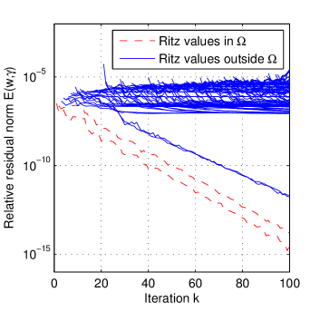
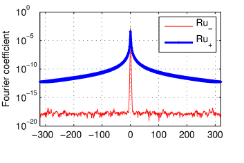
[] [] [] Figure 5: Absolute value of the eigenfunction [] Figure 6: Fourier coefficients decay of $u(x_{-},z)$ and $u(x_{+},z)$

Figure 4: Relative residual norm history

Figure 7: Execution of $m=100$ iterations of WTIAR. The parameters of the DtN maps are $x_{-}=0$ and $x_{+}=2/\pi+0.4$. The domain is discretized setting $n_{x}=640$ and $n_{z}=641$.

In Figure 7 we observe that the Fourier coefficients do not have exponential decay for $u(x_{+},z)$. Indeed, the decay is quadratic, which is consistent with the fact that the solutions are $C^{1}$-functions, but in general not $C^{2}$, as explained in Remark 1. In particular, the second derivative of the eigenfunction is not continuous in $x=x_{+}$. Hence, the eigenfunctions appear to have just weak regularity, which means that the waveguide eigenvalue problem does not have a strong solution. This supports the choice of the discretization method, based on the FEM, that we use in this paper. In these simulations we selected $x_{\pm}$ such that the enterior domain is minimized. We also carried out simulations for larger interior domains, without observing any qualitive difference in the computed solutions. By Remark 1, this suggests that the $C^{1}$-assumption is not a restriction in this case.

The plot of the absolute value of one eigenfunction is given in Figure 7. The convergence rate with respect to discretization, appears to be quadratic in the diameter of the elements. See Table 1.

Problem size	$n_{x}$	$n_{z}$	First eigenvalue	Second eigenvalue
132	10	11	-0.010297987 - 4.966269257i	-0.008202089 - 1.390972357i
462	20	21	-0.009556975 - 4.965939619i	-0.009012367 - 1.337899343i
1,722	40	41	-0.009401369 - 4.965933116i	-0.009258151 - 1.322687924i
6,642	80	81	-0.009368285 - 4.966067569i	-0.009332752 - 1.318511833i
26,082	160	161	-0.009359775 - 4.966072322i	-0.009350769 - 1.317465909i
103,362	320	321	-0.009357649 - 4.966071811i	-0.009355348 - 1.317202268i
411,522	640	641	-0.009357159 - 4.966073495i	-0.009356561 - 1.317134070i
1,642,242	1,280	1,281	-0.009357028 - 4.966073418i	-0.009356859 - 1.317117443i
6,561,282	2,560	2,561	-0.009356994 - 4.966073409i	-0.009356933 - 1.317113346i
9,009,002	3,000	3,001	-0.009356991 - 4.966073406i	-0.009356938 - 1.317112905i

Table 1: Eigenvalue approximations stemming from WTIAR with $m=100$.

As we mentioned in Remark 3.6, TIAR requires less memory and has the same complexity of IAR, although it is in practice considerable faster. According to section 4.2, WTIAR requires the same memory resources as TIAR, but WTIAR has lower complexity. These properties are illustrated in Figure 10 and Table 2.

[] []

Figure 8: CPU time needed to perform $m=100$ iterations of IAR, TIAR and WTIAR

[]

Figure 9: Difference between the matrices $H_{m}$ and Ritz values in $\Omega$ computed with IAR and WTIAR

Figure 10: Comparison between IAR, TIAR and the WTIAR in terms of CPU time and stability

			CPU time		storage of $Q_{m}$
$n$	$n_{x}$	$n_{z}$	IAR	WTIAR	IAR	TIAR
462	20	21	8.35 secs	2.58 secs	35.24 MB	7.98 MB
1,722	40	41	28.90 secs	2.83 secs	131.38 MB	8.94 MB
6,642	80	81	1 min and 59 secs	4.81 secs	506.74 MB	12.70 MB
26,082	160	161	8 mins and 13.37 secs	13.9 secs	1.94 GB	27.52 MB
103,362	320	321	out of memory	45.50 secs	out of memory	86.48 MB
411,522	640	641	out of memory	3 mins and 30.29 secs	out of memory	321.60 MB
1,642,242	1280	1281	out of memory	15 mins and 20.61 secs	out of memory	1.23 GB

Table 2: CPU time and estimated memory required to perform $m=100$ iterations of IAR and WTIAR. The memory requirements for the storage of the basis is the same TIAR and WTIAR.

As we showed in the theorem 3 TIAR and IAR are mathematically equivalent by construction. However, IAR and TIAR (as well as WTIAR) incorporate orthogonalization in different ways which may influence the impact of round-off errors. It turns out that the $H_{m}$ matrices computed with IAR and TIAR are numerically different, but the Ritz values in $\Omega$ have a small difference. See Figure 10. This suggests that there is an effect of the roundoff errors, but for the purpose of computing the Ritz values located in $\Omega$, such error is benign. Moreover, since TIAR requires less operations in the orthogonalization and implicitly imposes the structure, the roundoff errors might even be smaller for TIAR than IAR.

We mentioned in section 4.2, that when $n$ became sufficiently large, the dominating part of WTIAR is the orthogonalization process. This can be observed in Figure 13. Recall that the orthogonalization in WTIAR has complexity $\mathcal{O}(nm^{2})$, which is also the complexity of the standard Arnoldi algorithm.

[] [] []

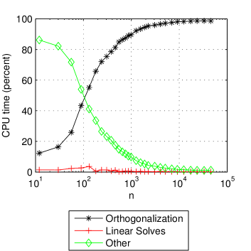
Figure 11: IAR

Figure 12: WTIAR

Figure 13: CPU time (percent) of the main parts of IAR and WTIAR with $m=100$ iterations.

Hence, solving the waveguide eigenvalue problem with WTIAR using a fine discretization, has in this sense the same complexity as solving a standard eigenvalue problem of the same size using the Arnoldi algorithm. According to remark 3.6 the dominating part of IAR is also the orthogonalization process, but this has higher complexity $\mathcal{O}(nm^{3})$. See Figure 13a.

5.2 Waveguide with complex shape

In order to show the generality of our algorithm, we carried out simulations on a waveguide with a more complex geometry and solutions. It is described in Figure 14 where $K_{1}=\sqrt{2.3}\omega$, $K_{2}=2\sqrt{3}\omega$, $K_{3}=4\sqrt{3}\omega$ and $K_{4}=\omega$ and $\omega=\pi$.

Figure 14: Geometry of the waveguide

We again select $x_{-}$ and $x_{+}$ such that the interior domain is minimized, i.e., $x_{-}=0$ and $x_{+}=2$. We discretize the problem and choose the same discretization parameters as in section 5.1 and choose as shift $\gamma_{0}=-2-i\pi$. An illustration of the execution of WTIAR, for this problem, is given in Figure 18, where the domain is discretized with $n_{x}=640$ and $n_{z}=641$ and $m=100$ iterations are performed. We observe that several Ritz values converge within the region of interest $\Omega$. See Figure 18 and Figure 18. One of the dominant eigenfunctions is illustrated in Figure 18.

[] [] []

Figure 15: Eigenvalues (converged Ritz values) and singularities

Figure 16: Relative residual norm history

[]

Figure 17: Absolute value of the eigenfunction

Figure 18: Execution of $m=100$ iterations of WTIAR. The parameters of the DtN maps are $x_{-}=0$ and $x_{+}=2$. The domain is discretized setting $n_{x}=640$ and $n_{z}=641$.

6 Concluding remarks and outlook

We have in this paper presented a new general approach for NEPs and shown how to specialize the method to a specific the waveguide eigenvalue problem stemming from analysis of wave propagation. Note that the non-polynomial nonlinearity stems from the absorbing boundary conditions. In our setting we were able establish an explicit characterization of the DtN maps, which allowed us to incorporate the structure at an algorithmic level. This approach does not appear to be restricted to the waveguide problem. Many PDEs can be constructed with absorbing boundary conditions expressed in a closed forms. By appropriate analysis, in particular differentiation with respect to the eigenvalue, the approach should carry over to other PDEs and other absorbing boundary conditions.

There exist several variants of IAR, e.g., the Chebyshev version [20] and restarting variations [19]. There are also related rational Krylov methods [4]. The results of this paper may also be extendable to these situations, although this would require further analysis. In particular, all of these methods require (in some way) a quantity corresponding to formula $y_{1}$ in (20), for which the problem-dependent structure must be incorporated. The computation of this quantity must be accurate and efficient and require considerable problem-specific attention.

Appendix A Proof of Lemma 2

We consider the exterior problem on $S_{+}$ in (11). The proof corresponding to $S_{-}$ is analogous. To simplify the notation we write $\beta_{k}=\beta_{+,k}(\gamma)$ and assume, without loss of generality, that $x_{+}=0$. By Remark 1 the solutions of (11) are in $C^{1}$ and every vertical trace can then be expanded in a Fourier series. Therefore we can express

$$w(x,z)=\sum_{k\in{\mathbb{Z}}}w_{k}(x)e^{2\pi ikz},\qquad g(z)=\sum_{k\in{\mathbb{Z}}}g_{k}e^{2\pi ikz}.$$

By again using Remark 1, we have that the solutions to the exterior problem are in $C^{\infty}$ if $x>0$ and satisfy (11a). Therefore, the coefficients $w_{k}$ satisfy

$$\sum_{k\in{\mathbb{Z}}}\left(w_{k}^{\prime\prime}-(2\pi k)^{2}w_{k}+4\pi\gamma iw_{k}+(\gamma^{2}+\kappa_{+}^{2})w_{k}\right)e^{2\pi ikz}=\sum_{k\in{\mathbb{Z}}}\left(w_{k}^{\prime\prime}+\beta_{k}w_{k}\right)e^{2\pi ikz}=0,$$

where $\beta_{k}$ is given in (9). Thus, in order for $w$ to satisfy (11a), we have

$$w_{k}^{\prime\prime}+\beta_{k}w_{k}=0,$$

for all $k$. We now claim that there are constants $C,C^{\prime}$ independent of $k$ such that

(49) $$|\beta_{k}|\leq C(1+(2\pi k)^{2}),\qquad|\operatorname{Im}\sqrt{\beta_{k}}|\geq C^{\prime}\sqrt{1+(2\pi k)^{2}}.$$

In particular, $\beta_{k}\neq 0$ and

$$w_{k}(x)=c_{k}e^{i{\operatorname{sign}}(\operatorname{Im}(\beta_{k}))\sqrt{\beta_{k}}x}+d_{k}e^{-i{\operatorname{sign}}(\operatorname{Im}(\beta_{k}))\sqrt{\beta_{k}}x}.$$

To determine $c_{k}$ and $d_{k}$ we have two boundary conditions. First, since $w\in H^{1}(S_{+})$, then $|w_{k}(x)|$ can not grow as $x\to\infty$. This means that $d_{k}=0$. Second, at $x=0$, we have $w(0,z)=g(z)$, so $c_{k}=g_{k}$. Hence, we have the explicit solution

$$w_{k}(x)=g_{k}e^{i{\operatorname{sign}}(\operatorname{Im}(\beta_{k}))\sqrt{\beta_{k}}x}.$$

Existence is thus proved, and the relationship (13) for the DtN maps follows directly for this solution by differentiating $w_{k}(x)$ and evaluating at $x=0$. We also have ${\mathcal{T}}_{+,\gamma}[g]\in L^{2}(0,1)$ since

$$||{\mathcal{T}}_{+,\gamma}[g]||^{2}_{L^{2}(0,1)}=\sum_{k\in{\mathbb{Z}}}|\beta_{k}|\,|g_{k}|^{2}\leq C\sum_{k\in{\mathbb{Z}}}(1+(2\pi k)^{2})\,|g_{k}|^{2}=C||g||_{H^{1}([0,1])}.$$

Finally, the estimate (12) is given by

$$||w||_{H^{1}(S_{+})}^{2} =||w||_{L^{2}(S_{+})}^{2}+||\nabla w||_{L^{2}(S_{+})}^{2}=\sum_{k\in{\mathbb{Z}}}\left[\left(1+(2\pi k)^{2}\right)||w_{k}||_{L^{2}(0,\infty)}^{2}+||w^{\prime}_{k}||_{L^{2}(0,\infty)}^{2}\right]$$

$$=\sum_{k\in{\mathbb{Z}}}|g_{k}|^{2}\left(1+(2\pi k)^{2}+|\beta_{k}|\right)\int_{0}^{\infty}e^{-2{\operatorname{sign}}(\operatorname{Im}(\beta_{k}))\operatorname{Im}\sqrt{\beta_{k}}x}dx$$

$$=\sum_{k\in{\mathbb{Z}}}\frac{|g_{k}|^{2}}{2|\operatorname{Im}\sqrt{\beta_{k}}|}\left(1+(2\pi k)^{2}+|\beta_{k}|\right)\leq\frac{C+1}{2C^{\prime}}\sum_{k\in{\mathbb{Z}}}|g_{k}|^{2}\sqrt{1+(2\pi k)^{2}}$$

$$=\frac{C+1}{2C^{\prime}}||g||_{H^{1/2}([0,1])}^{2}.$$

Uniqueness follows from this estimate. It remains to show the claim (49). The estimate for $|\beta_{k}|$ is straightforward. For the second estimate we note that $|\operatorname{Im}\beta_{k}|=2|\operatorname{Re}\gamma(2\pi k+\operatorname{Im}\gamma)|\neq 0$ for all $k$ from the assumptions $\operatorname{Im}\gamma\not\in 2\pi\mathbb{Z}$ and $\operatorname{Re}\gamma\neq 0$. It follows that also $\operatorname{Im}\sqrt{\beta}_{k}\neq 0$ for all $k$ and since

$$\lim_{|k|\to\infty}a_{k}:=\lim_{|k|\to\infty}\frac{\operatorname{Im}\sqrt{\beta_{k}}}{\sqrt{1+(2\pi k)^{2}}}=\operatorname{Im}\sqrt{\lim_{|k|\to\infty}\frac{\beta_{k}}{1+(2\pi k)^{2}}}=1,$$

the sequence $\{1/a_{k}\}$ is bounded. Hence, there is a $C^{\prime}$ such that (49) holds, which concludes the proof.

Appendix B Matrices of the FEM–discretization

The matrices $(A_{i})_{i=0}^{2}$ and $(C_{1,i})_{i=0}^{2}$ are stem from to the Ritz–Galerkin discretization of the bilinear forms $a,b$ and $c$. They can be decomposed and expressed as

$$A_{0} :=D_{xx}+D_{zz}+K, C_{1,0} :=\tilde{D}_{xx}+\tilde{D}_{zz}+\tilde{K},$$

$$A_{1} :=2D_{z}, C_{1,1} :=2\tilde{D}_{z},$$

$$A_{2} :=B, C_{1,2} :=\tilde{B}.$$

Now we need to define the following tridiagonal Toeplitz matrices. Let $E_{m}$ be the tridiagonal Toeplitz matrix with diagonals consisting of $e_{i+1,i}=-1$, $e_{i,i}=2$ and $e_{i,i+1}=-1$. Let $F_{m}$ be the tridiagonal Toeplitz matrix with diagonals consisting of $f_{i+1,i}=1$, $f_{i,i}=4$ and $f_{i,i+1}=1$. Let $G_{m}$ be the anti-symmetric tridiagonal Toeplitz matrix consisting of $g_{i+1,i}=1$, $g_{i,i}=0$ and $g_{i,i+1}=-1$.

Then, we have

$$D_{xx}=-\frac{h_{z}}{6h_{x}}E_{n_{x}}\otimes\left(B_{n_{z}}+e_{n_{z}}e_{1}^{T}+e_{1}e_{n_{z}}^{T}\right), \tilde{D}_{xx}=-\frac{h_{z}}{6h_{x}}-(e_{1},e_{n_{x}})\otimes\left(F_{n_{z}}+e_{n_{z}}e_{1}^{T}+e_{1}e_{n_{z}}^{T}\right),$$

$$D_{zz}=-\frac{h_{x}}{6h_{z}}F_{n_{x}}\otimes\left(E_{n_{z}}-e_{n_{z}}e_{1}^{T}-e_{1}e_{n_{z}}^{T}\right), \tilde{D}_{zz}=-\frac{h_{x}}{6h_{z}}(e_{1},e_{n_{x}})\otimes\left(E_{n_{z}}-e_{n_{z}}e_{1}^{T}-e_{1}e_{n_{z}}^{T}\right),$$

$$D_{z}=-\frac{h_{x}}{12}F_{n_{x}}\otimes\left(G_{n_{z}}+e_{n_{z}}e_{1}^{T}-e_{1}e_{n_{z}}^{T}\right), \tilde{D}_{z}=-\frac{h_{x}}{12}(e_{1},e_{n_{x}})\otimes\left(G_{n_{z}}+e_{n_{z}}e_{1}^{T}-e_{1}e_{n_{z}}^{T}\right),$$

$$B=\frac{h_{x}h_{z}}{36}G_{n_{x}}\otimes\left(G_{n_{z}}+e_{n_{z}}e_{1}^{T}-e_{1}e_{n_{z}}^{T}\right), \tilde{B}=\frac{h_{x}h_{z}}{36}(e_{1},-e_{n_{x}})\otimes\left(G_{n_{z}}+e_{n_{z}}e_{1}^{T}-e_{1}e_{n_{z}}^{T}\right).$$

The matrices $K$ and $\tilde{K}$ arise from the Ritz–Galerkin discretization of the bilinear form

$$f(u,v)=\int_{0}^{1}\int_{x_{-}}^{x_{+}}\kappa(x,z)^{2}u(x,z)v(x,z)\ dx\ dz.$$

The elements of such matrices are obtained integrating the product of two basis functions against the square of the wavenumber. We can split the integral over the elements. Recall that $\kappa(x,z)$ is piecewise constant, then the final task is to compute, for each element, the integral of a piecewise polynomial function. Such integral is given in an explicit form by quadrature formulas.

Appendix C Computation of the derivatives in DtN-map

In the computation of $y_{1}$ described in section 4.2, we need the coefficients $\alpha_{\pm,j,\ell}$. They can be computed with the following three-term recurrence.

Lemma 13 (Recursion for $\alpha_{\pm,j,\ell}$).

Suppose $\gamma_{0}\not\in i\mathbb{R}$. Then the coefficients in (43) are explicitly given by

(50) $$\begin{cases}\alpha_{\pm,j,0}=iw_{j}f_{\pm,j,0}+d_{0}&\\ \alpha_{\pm,j,1}=iw_{j}f_{\pm,j,1}-d_{0}&\\ \alpha_{\pm,j,\ell}=iw_{j}f_{\pm,j,\ell}\ell!&\ell\geq 2,\\ \end{cases}$$

where coefficients $f_{\pm,j,\ell}$ satisfy the following three-term recurrence

(51) $$\begin{cases}\displaystyle f_{\pm,j,\ell}=-\frac{2a_{\pm,j}(\ell-3)f_{\pm,j,\ell-2}+b_{\pm,j}(2\ell-3)f_{\pm,j,\ell-1}}{2\ell c_{\pm,j}}&\ell\geq 2,\\ \displaystyle f_{\pm,j,0}=\sqrt{c_{\pm,j}},\\ \displaystyle f_{\pm,j,1}=\frac{b_{\pm,j}}{2\sqrt{c_{\pm,j}}},\\ \end{cases}$$

with

$$\begin{cases}\displaystyle a_{\pm,j}=\conj{\gamma_{0}}^{2}-4\pi ij\conj{\gamma_{0}}-4\pi^{2}j^{2}+\kappa_{\pm}^{2},\\ b_{\pm,j}=2\gamma_{0}\conj{\gamma_{0}}+4\pi ij(\conj{\gamma_{0}}-\gamma_{0})+8\pi^{2}j^{2}-2\kappa_{\pm}^{2},\\ c_{\pm,j}=4\pi ij\gamma_{0}-4\pi^{2}j^{2}+\kappa_{\pm}^{2}+\gamma_{0}^{2},\\ w_{j}={\operatorname{sign}}\left(\operatorname{Re}(\gamma_{0})\left(\operatorname{Im}(\gamma_{0})+2\pi j\right)\right).\end{cases}$$

Proof C.7.

By definition (43)

$$\alpha_{\pm,j,\ell}=\left(\frac{d^{\ell}}{d\lambda^{\ell}}\left((1-\lambda)s_{\pm,j}\left(\frac{\gamma_{0}+\lambda\conj{\gamma}_{0}}{1-\lambda}\right)\right)\right)_{\lambda=0}+\left(\frac{d^{\ell}}{d\lambda^{\ell}}\left((1-\lambda)d_{0}\right)\right)_{\lambda=0}.$$

The computation of the second term is straightforward. The first term can be computed as follows. In order to compute the derivatives in zero, we now derive formulas for the Taylor expansion

$$(1-\lambda)s_{\pm,j}\left(\frac{\gamma_{0}+\lambda\conj{\gamma}_{0}}{1-\lambda}\right)=\sum_{\ell=0}^{+\infty}f_{\pm,j,\ell}\lambda^{\ell}.$$

Since all functions are analytic in the origin, there exists a neighborhood of the origin $N$, such that when $\lambda\in N$,

$$(1-\lambda)s_{\pm,j}\left(\frac{\gamma_{0}+\lambda\conj{\gamma}_{0}}{1-\lambda}\right)=w_{j}\sqrt{a_{\pm,j}\lambda^{2}+b_{\pm,j}\lambda+c_{\pm,j}}.$$

Hence, we have reduced the problem to computing the power series expansion of $\sqrt{a_{\pm,j}\lambda^{2}+b_{\pm,j}\lambda+c_{\pm,j}}$. To this end we use the well known formula involving the Gegenbauer polynomials and their generating function. See e.g. [27]. We have that

$$\sqrt{a_{\pm,j}\lambda^{2}+b_{\pm,j}\lambda+c_{\pm,j}} =\sqrt{c_{\pm,j}}\left[\left(\sqrt{\frac{a_{\pm,j}}{c_{\pm,j}}}\lambda\right)^{2}+\frac{b_{\pm,j}}{\sqrt{a_{\pm,j}c_{\pm,j}}}\left(\sqrt{\frac{a_{\pm,j}}{c_{\pm,j}}}\lambda\right)+1\right]^{-\frac{1}{2}}$$

$$=\sum_{\ell=0}^{+\infty}\sqrt{\frac{a_{\pm,j}^{\ell}}{c_{\pm,j}^{\ell-1}}}C_{\ell}^{(-1/2)}\left(-\frac{b_{\pm,j}}{2\sqrt{a_{\pm,j}c_{\pm,j}}}\right)\lambda^{\ell},$$

where $C_{\ell}$ is the $\ell$-th Gegenbauer polynomial. Consequently, the coefficients in the power series expansion are

$$f_{\pm,j,\ell}=\sqrt{\frac{a_{\pm,j}^{\ell}}{c_{\pm,j}^{\ell-1}}}C_{\ell}^{(-1/2)}\left(-\frac{b_{\pm,j}}{2\sqrt{a_{\pm,j}c_{\pm,j}}}\right).$$

The recursion (51) follows from substitution of the recursion formula for Gegenbauer polynomials.

References

- [1] Z. Bai, Y. Su, SOAR: A second-order Arnoldi method for the solution of the quadratic eigenvalue problem, SIAM J. Matrix Anal. Appl. 26 (3) (2005) 640–659.
- [2] G. Bao, Finite element approximation of time harmonic waves in periodic structures, SIAM J. Numer. Anal. 32 (4) (1995) 1155–1169.
- [3] R. V. Beeumen, E. Jarlebring, W. Michiels, A rank-exploiting infinite Arnoldi algorithm for nonlinear eigenvalue problems, Tech. rep., Tech. Report, submitted for publication (2014).
- [4] R. V. Beeumen, K. Meerbergen, W. Michiels, A rational Krylov method based on Hermite interpolation for nonlinear eigenvalue problems, SIAM J. Sci. Comput. 35 (1) (2013) A327–A350.
- [5] R. V. Beeumen, K. Meerbergen, W. Michiels, Compact rational Krylov methods for nonlinear eigenvalue problems, Tech. Rep. 541, KU Leuven (2014).
- [6] J.-P. Berenger, A perfectly matched layer for the absorption of electromagnetic waves, J. Comput. Phys. 114 (2) (1994) 185–200.
- [7] T. Betcke, N. J. Higham, V. Mehrmann, C. Schröder, F. Tisseur, NLEVP: A collection of nonlinear eigenvalue problems, ACM Trans. Math. Softw. 39 (2) (2013) 1–28.
- [8] D. Bindel, S. Govindjee, Elastic PMLs for resonator anchor loss simulation, Int. J. Numer. Methods Eng. 64 (6) (2005) 789–818.
- [9] J. Butler, W. Ferguson, G. A. Evans, P. J. Stabile, A. Rosen, A boundary element technique applied to the analysis of waveguides with periodic surface corrugations, IEEE J. of quantum electronics 28 (7) (1992) 1701–1709.
- [10] C. Effenberger, D. Kressner, Chebyshev interpolation for nonlinear eigenvalue problems, BIT 52 (4) (2012) 933–951.
- [11] C. Effenberger, D. Kressner, C. Engström, Linearization techniques for band structure calculations in absorbing photonic crystals, Int. J. Numer. Methods Eng. 89 (2) (2012) 180–191.
- [12] C. Engström, Spectral approximation of quadratic operator polynomials arising in photonic band structure calculations, Numer. Math. 126 (3) (2014) 413–440.
- [13] L. C. Evans, Partial differential equations. 2nd ed, American mathematical society, 2010.
- [14] S. Fliss, A Dirichlet-to-Neumann approach for the exact computation of guided modes in photonic crystal waveguides, SIAM J. Sci. Comput. 35 (2) (2013) B438–B461.
- [15] D. Givoli, I. Patlashenko, Dirichlet-to-Neumann boundary condition for time-dependent dispersive waves in three-dimensional guides, J. Comput. Phys. 199 (1) (2004) 339–354.
- [16] T. Hagstrom, New results on absorbing layers and radiation boundary conditions, Ainsworth, Mark (ed.) et al., Topics in computational wave propagation. Direct and inverse problems. Berlin: Springer. Lect. Notes Comput. Sci. Eng.
- [17] I. Harari, I. Patlashenko, D. Givoli, Dirichlet-to-Neumann maps for unbounded wave guides, J. Comput. Phys. 143 (1) (1998) 200–223.
- [18] E. Jarlebring, K. Meerbergen, W. Michiels, A Krylov method for the delay eigenvalue problem, SIAM J. Sci. Comput. 32 (6) (2010) 3278–3300.
- [19] E. Jarlebring, K. Meerbergen, W. Michiels, Computing a partial Schur factorization of nonlinear eigenvalue problems using the infinite Arnoldi method, SIAM J. Matrix Anal. Appl. 35 (2) (2014) 411–436.
- [20] E. Jarlebring, W. Michiels, K. Meerbergen, A linear eigenvalue algorithm for the nonlinear eigenvalue problem, Numer. Math. 122 (1) (2012) 169–195.
- [21] L. Kaufman, Eigenvalue problems in fiber optic design, SIAM J. Matrix Anal. Appl. 28 (1) (2006) 105–117.
- [22] J. B. Keller, D. Givoli, Exact non-reflecting boundary conditions, J. Comput. Phys. 82 (1) (1989) 172–192.
- [23] D. Kressner, J. Roman, Memory-efficient Arnoldi algorithms for linearizations of matrix polynomials in Chebyshev basis, Numer. Linear Algebra Appl. 21 (4) (2014) 569–588.
- [24] B.-S. Liao, Z. Bai, L.-Q. Lee, K. Ko, Nonlinear Rayleigh-Ritz iterative method for solving large scale nonlinear eigenvalue problems, Taiwanese Journal of Mathematics 14 (3) (2010) 869–883.
- [25] V. Mehrmann, H. Voss, Nonlinear eigenvalue problems: A challenge for modern eigenvalue methods, GAMM-Mitt. 27 (2004) 121–152.
- [26] S. T. Peng, T. Tamir, H. L. Bertoni, Theory of periodic dielectric waveguides, IEEE Trans. Microwave Theory and Techniques 1 (1975) 123–133.
- [27] A. D. Polyanin, A. V. Manzhirov, Handbook of mathematics for engineers and scientists, CRC Press, 2006.
- [28] D. Stowell, J. Tausch, Variational formulation for guided and leaky modes in multilayer dielectric waveguides, Commun. Comput. Phys. 7 (3) (2010) 564–579.
- [29] Y. Su, Z. Bai, Solving rational eigenvalue problems via linearization, SIAM J. Matrix Anal. Appl. 32 (1) (2011) 201–216.
- [30] J. Tausch, Computing Floquet-Bloch modes in biperiodic slabs with boundary elements, J. Comput. Appl. Math. 254 (2013) 192–203.
- [31] J. Tausch, J. Butler, Floquet multipliers of periodic waveguides via Dirichlet-to-Neumann maps, J. Comput. Phys. 159 (1) (2000) 90–102.
- [32] H. Voss, Nonlinear eigenvalue problems, in: L. Hogben (ed.), Handbook of Linear Algebra, Second Edition, No. 164 in Discrete Mathematics and Its Applications, Chapman and Hall/CRC, 2013.
- [33] H. Voss, K. Yildiztekin, X. Huang, Nonlinear low rank modification of a symmetric eigenvalue problem, SIAM J. Matrix Anal. Appl. 32 (2) (2011) 515–535.
- [34] Y. Zhang, Y. Su, A memory-efficient model order reduction for time-delay systems, BIT 53 (2013) 1047–1073.