Quantum–mechanical picture of peripheral chiral dynamics

Abstract

The nucleon’s peripheral transverse charge and magnetization densities are computed in chiral effective field theory. The densities are represented in first–quantized form, as overlap integrals of chiral light–front wave functions describing the transition of the nucleon to soft pion–nucleon intermediate states. The orbital motion of the pion causes a large left–right asymmetry in a transversely polarized nucleon. The effect attests to the relativistic nature of chiral dynamics [pion momenta $k=O(M_{\pi})$] and could be observed in form factor measurements at low momentum transfer.

The long–distance behavior of strong interactions is governed by the spontaneous breaking of chiral symmetry in the microscopic theory of Quantum Chromodynamics. The associated Goldstone bosons — the pions — are almost massless on the hadronic scale, couple weakly to other hadrons (proportional to their momentum), and mediate long–distance interactions. The resulting “chiral dynamics” can be studied systematically using methods of effective field theory (EFT) Gasser:1983yg ; Weinberg:1990rz and explains numerous phenomena in low–energy pion–pion and pion–nucleon scattering, the nucleon–nucleon interaction at large distances, and electroweak interactions of hadrons.

Chiral dynamics represents an essentially relativistic dynamical system, as the pion 4–momenta in typical processes are of the order of the pion mass, $k=O(M_{\pi})$ Gasser:1983yg , and the number of particles changes due to quantum fluctuations. Chiral EFT is therefore usually formulated and solved as a second–quantized field theory. While this allows one to calculate most observables of interest, for many purposes it would be desirable to have a first–quantized, particle–based formulation of the dynamics. It would make it possible to follow the space–time evolution of chiral processes and gain a more intuitive understanding of their effects. It would introduce the concept of a wave function and its densities and help quantify the spatial structure of hadrons, the orbital motion of pions, and polarization effects.

The light–front (LF) formulation of relativistic dynamics Dirac:1949cp ; Leutwyler:1977vy ; Brodsky:1997de makes it possible to construct a consistent first–quantized description of essentially relativistic systems. In this framework one follows the evolution of the system in LF time $x^{+}=x^{0}+x^{3}\equiv t+z$. The wave functions at fixed $x^{+}$ are invariant under Lorentz boosts in the longitudinal ($z-$) direction, so that their particle content and densities are frame–independent and have objective meaning — in contrast to the equal–time wave function, where they are frame–dependent. Transverse boosts (in the $x,y$–plane) are kinematical and preserve the particle number. Orbital motion and spin are naturally expressed and lead to a description in close correspondence to non-relativistic quantum mechanics Brodsky:1997de .

In this work we use chiral EFT in the LF formulation to compute the long–distance contributions to the nucleon’s electromagnetic current matrix element and explain their properties. The form factors are expressed in terms of the transverse densities of charge and magnetization at fixed LF time Soper:1976jc ; Burkardt:2000za ; Burkardt:2002hr ; Miller:2007uy . We calculate the isovector densities at peripheral transverse distances $b=O(M_{\pi}^{-1})$ using chiral EFT in the leading–order (LO) approximation. We represent the densities in first–quantized form, as overlap integrals of chiral LF wave functions describing the transition of the nucleon to soft pion–nucleon intermediate states. The new representation leads to a simple quantum–mechanical picture, according to which the orbital motion of the soft pion causes a left-right asymmetry of the “plus” current density in a transversely polarized nucleon Burkardt:2002hr . The effect is sizable and attests to the essentially relativistic nature of chiral dynamics. Details will be presented elsewhere long .

The transition matrix element of the electromagnetic current between nucleon states with 4–momenta $p_{1}$ and $p_{2}$ is parametrized by the Dirac and Pauli form factors, $F_{1}(t)$ and $F_{2}(t)$, which are functions of the invariant momentum transfer $t\equiv\Delta^{2}=(p_{2}-p_{1})^{2}$ (we follow the notation of Ref. Granados:2013moa ). In a frame where the momentum transfer is transverse, $\bm{\Delta}_{T}\equiv(\Delta^{x},\Delta^{y})\neq 0,\,\Delta^{0}=\Delta^{z}=0$, the form factors are represented as a Fourier integral over a transverse coordinate $\bm{b}\equiv(b^{x},b^{y})$ Burkardt:2000za ; Miller:2007uy

$$F_{1,2}(t=-\bm{\Delta}_{T}^{2})\;\;=\;\;\int d^{2}b\;e^{i\bm{\Delta}_{T}\cdot\bm{b}}\;\rho_{1,2}(b).$$ (1)

The functions $\rho_{1,2}(b\equiv|\bm{b}|)$ describe the transverse spatial distribution of charge and magnetization in the nucleon at fixed LF time. Specifically, in a state where the nucleon is localized in transverse space at the origin, and spin–polarized in the $y$–direction, the expectation value of the current $J^{+}\equiv J^{0}+J^{3}$ at LF time $x^{+}=0$ and transverse position $\bm{x}_{T}=\bm{b}$ is

$$\langle J^{+}(\bm{b})\rangle_{\text{\scriptsize loc}} = (...)[\rho_{1}(b)\;+\;(2S^{y})\,\cos\phi\,\widetilde{\rho}_{2}(b)],$$ (2)

$$\widetilde{\rho}_{2}(b) \equiv \frac{\partial}{\partial b}\left[\frac{\rho_{2}(b)}{2M_{N}}\right],$$ (3)

where $(...)$ hides a trivial factor arising from the normalization of states, $\cos\phi\equiv b^{x}/b$, and $S^{y}=\pm 1/2$ is the $y$–spin projection in the nucleon rest frame (see Fig. 1) Burkardt:2000za ; Granados:2013moa . Thus $\rho_{1}(b)$ describes the spin–independent (left–right symmetric) and $\cos\phi\,\widetilde{\rho}_{2}(b)$ the spin–dependent (left–right antisymmetric) plus current in the $y$–polarized nucleon. Choosing $S^{y}=+1/2$ and looking at two opposite points on the $x$–axis, $\bm{b}=\mp b\bm{e}_{x}$, one has

$$\langle J^{+}(\mp b\bm{e}_{x})\rangle_{\text{\scriptsize loc}} = (...)\;[\rho_{1}(b)\,\mp\,\widetilde{\rho}_{2}(b)]$$ (4)

$$\equiv (...)\;\rho_{\rm left/right}(b),$$

which shows that $\rho_{1}(b)$ and $\widetilde{\rho}_{2}(b)$ can be determined directly as the left–right symmetric and antisymmetric parts of the plus current on the $x$–axis.

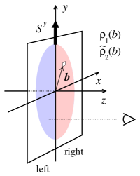
Figure 1: Interpretation of the transverse densities in a nucleon state polarized in the $y$–direction, Eq. (2).

At peripheral distances $b=O(M_{\pi}^{-1})$ the transverse densities are governed by chiral dynamics and can be computed from first principles using chiral EFT Granados:2013moa ; Strikman:2010pu . The densities can be obtained from the relativistic chiral EFT results for the form factors Gasser:1987rb ; Bernard:1992qa ; Kubis:2000zd . Peripheral contributions arise from the chiral processes in which the current couples to the nucleon through two–pion exchange, i.e., contributions to the two–pion cut of the isovector form factors at $t>4M_{\pi}^{2}$. At LO these are given by the Feynman diagrams of Fig. 2a, where the vertices are those of the relativistic chiral Lagrangian Becher:1999he . The first diagram contains a term in which the pole of the intermediate nucleon propagator is canceled by the numerator; this term is of the same form as the contact term from the second diagram and can be combined with it. Effectively this amounts to replacing the $\pi NN$ vertices in the first diagram by the pseudoscalar vertex $M_{N}g_{A}\gamma_{5}/F_{\pi}$, and changing the $\pi\pi NN$ contact coupling in the second as $1/F_{\pi}^{2}\rightarrow(1-g_{A}^{2})/F_{\pi}^{2}$ Strikman:2010pu ; Granados:2013moa .

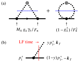
Figure 2: (a) Feynman diagrams of LO chiral EFT processes contributing to the peripheral transverse densities (two–pion cut of the form factors). Indicated below are the effective vertices obtained after isolating the nucleon pole term of the first diagram. (b) Chiral LF wave function of the nucleon.

With this rearrangement the first Feynman diagram is given entirely by the nucleon pole contribution. It can therefore be represented as a LF time–ordered process in which the initial nucleon makes a transition to a soft pion–nucleon intermediate state and back long . The transition is described by the chiral LF wave function (Fig. 2b)

$$\Psi(y,\bm{k}_{T};\,\textrm{pol}) \equiv \frac{\Gamma(y,\bm{k}_{T};\,\textrm{pol})}{\Delta\mathcal{M}^{2}(y,\bm{k}_{T})},$$ (5)

where $y=k^{+}/p_{1}^{+}$ is the LF plus momentum fraction of the pion, $\bm{k}_{T}$ its transverse momentum relative to the initial nucleon with $\bm{p}_{1T}=0$, and “pol” denotes generic spin quantum numbers characterizing the initial and intermediate nucleon. In the numerator $\Gamma$ is the on-shell pseudoscalar $\pi NN$ vertex between the initial nucleon and the intermediate one with LF momentum $(1-y)p_{1}^{+}$ and $-\bm{k}_{T}$. In the denominator $\Delta\mathcal{M}^{2}$ denotes the invariant mass difference between the initial and intermediate state,

$$\Delta\mathcal{M}^{2}(y,\bm{k}_{T}) \equiv [\bm{k}_{T}^{2}+M_{T}^{2}(y)]/[y(1-y)],$$ (6)

$$M_{T}^{2}(y) \equiv (1-y)M_{\pi}^{2}+y^{2}M_{N}^{2},$$ (7)

which is proportional to the LF energy denominator of the transition Brodsky:1997de . The wave function for a state moving with overall transverse momentum $\bm{p}_{1T}\neq 0$ is obtained by a transverse boost, and analogous formulas describe the transition back to the final state with $\bm{p}_{2T}$. The chiral wave functions refer to the parametric regime $|\bm{k}_{T}|=O(M_{\pi})$ and $y=O(M_{\pi}/M_{N})$, where the pion is soft and couples weakly to the nucleon, and are used in this context only. The coordinate–space wave function is

$$\Phi(y,\bm{r}_{T},\,\textrm{pol}) \equiv \int\frac{d^{2}k_{T}}{(2\pi)^{2}}\;e^{i\bm{k}_{T}\cdot\bm{r}_{T}}\;\Psi(y,\bm{k}_{T};\,\textrm{pol}),$$ (8)

where $\bm{r}_{T}$ is the transverse separation of the pion–nucleon system in the intermediate state and $|\bm{r}_{T}|=O(M_{\pi}^{-1})$.

The peripheral transverse densities can be expressed as overlap integrals of the chiral LF wave functions of the initial and final nucleon and an effective contact term long . A particularly simple form is obtained when the nucleon spin states in the wave function are quantized in the transverse $y$–direction. Transversely polarized LF spinors are constructed by preparing a transverse spinor in the nucleon rest frame and performing a longitudinal and a transverse boost to get to the desired LF momentum Brodsky:1997de . We denote the LF wave function Eq. (8) definied with such transversely polarized nucleon spin states by

$$\Phi_{\rm tr}(y,\bm{r}_{T};\tau,\tau_{1}),$$ (9)

where $\tau_{1}$ and $\tau$ are the $y$–spin quantum numbers of the initial and the intermediate nucleon states; the complex conjugate function $\Phi^{\ast}_{\rm tr}(y,\bm{r}_{T};\tau,\tau_{2})$ describes the transition back to the final state with $y$–spin $\tau_{2}$. At the special points $\bm{b}=\mp b\bm{e}_{x}$ [cf. Eq. (4)] only the transverse spin–flip wave function ($\tau_{1}=\tau_{2}=+1/2,\tau=-1/2$) contributes to the current matrix element; the spin–nonflip wave function ($\tau=+1/2$) vanishes on the transverse $x$–axis. We obtain the isovector densities as [$\rho^{V}\equiv(\rho^{p}-\rho^{n})/2$]

$$\left.\begin{array}[]{l}\rho_{\rm left}^{V}(b)\\[2.15277pt] \rho_{\rm right}^{V}(b)\end{array}\right\} = \int_{0}^{1}\!dy\,\frac{|\Phi_{\rm tr}(y,\mp r_{T}\bm{e}_{x};-\frac{1}{2},\frac{1}{2})|^{2}}{2\pi y(1-y)^{3}}$$ (13)

$$[r_{T}=b/(1-y)].$$

The explicit expressions for the spin–flip wave function at large separations $r_{T}\gg M_{T}^{-1}$ are [cf. Eq. (7)]

$$\Phi_{\rm tr}(y,\mp r_{T}\bm{e}_{x};-{\textstyle\frac{1}{2}},{\textstyle\frac{1}{2}})$$ (14)

$$= \frac{g_{A}M_{N}\,y\sqrt{1-y}}{2\sqrt{2\pi}F_{\pi}}\,\left[-yM_{N}\mp M_{T}(y)\right]\;\,\frac{e^{-M_{T}(y)r_{T}}}{\sqrt{M_{T}(y)r_{T}}};\hskip 20.00003pt$$

exact expression are given in Ref. long . The charge and magnetization densities are then obtained as

$$\left.\begin{array}[]{l}\rho^{V}_{1}(b)\\[2.15277pt] \widetilde{\rho}_{2}^{V}(b)\end{array}\right\}\;\;=\;\;\frac{1}{2}[\pm\rho_{\rm left}^{V}(b)+\rho_{\rm right}^{V}(b)].$$ (15)

The effective contact term in Fig. 2 describes the instantaneous contributions to the current in LF time (zero modes) and has to be added to Eq. (13). The coupling $\propto(1-g_{A}^{2})$ shows that this term reflects the nucleon’s internal structure due to non-chiral intermediate states long ; Granados:2013moa . Its contribution to the density is left–right symmetric and amounts to $<$10% of $\rho_{1}^{V}(b)$ at $b>1\,M_{\pi}^{-1}$. The peripheral densities are thus practically determined by the wave function overlap Eq. (13).

Figure 3: Left and right peripheral transverse densities in LO chiral EFT, as given by Eq. (13) and the contact term. The plot shows the densities after extraction of the exponential factor $\exp(-2M_{\pi}b)$. The transverse distance $b$ and the densities are given in units of the pion mass.

The LF representation Eq. (13) (including the contact term) is exactly equivalent to the result of the relativistically invariant EFT calculation Granados:2013moa and embodies the entire chiral structure of the peripheral densities at LO. It reveals several interesting properties: (a) The left and right densities are of the same parametric order in the heavy–baryon limit, $\rho^{V}_{\rm left}(b)/\rho^{V}_{\rm right}(b)=O(1)$ for $M_{\pi}/M_{N}\rightarrow 0$, because the integral in Eq. (13) is dominated by pion momentum fractions $y=O(M_{\pi}/M_{N})$. (b) The left and right densities in Eq. (13) are individually positive, $\rho_{\rm left/right}^{V}(b)>0$. The charge and magnetization densities Eq. (15) therefore obey an inequality,

$$|\widetilde{\rho}_{2}^{V}(b)|\;<\;\rho_{1}^{V}(b),$$ (16)

as was observed numerically in Ref. Granados:2013moa . (c) The left-right asymmetry of the densities produced by chiral dynamics is numerically large (see Fig. 3). The ratio $\rho^{V}_{\rm left}(b)/\rho^{V}_{\rm right}(b)$ is $\sim$10 at $b=1M_{\pi}^{-1}$ and decreases slowly at larger distances. As a result the charge and magnetization densities Eq. (15) are almost equal and opposite,

$$\widetilde{\rho}_{2}^{V}(b)\;\approx\;-\rho_{1}^{V}(b),$$ (17)

and the inequality Eq. (16) is almost saturated.

Our findings can be summarized in a simple quantum–mechanical picture of the peripheral transverse densities in chiral EFT (see Fig. 4), inspired by the general arguments of Ref. Burkardt:2002hr . Consider a physical proton with $y$–spin projection $+1/2$ in the rest frame. In the interaction picture we may think of this system as a bare nucleon that undergoes transitions to multiple pion–nucleon states through the chiral EFT interactions. In LO the peripheral left/right densities (at the points $\bm{b}=\mp b\bm{e}_{x}$) arise from the single $\pi^{+}n$ intermediate state, in which the neutron has $y$–spin $-1/2$ and the pion is in a state with orbital angular momentum $L=1$ and $y$–projection $L^{y}=+1$. Because of the orbital motion the pion on the left moves toward the observer and has net positive $z$–momentum $k^{z}>0$, while the pion on the right moves away and has $k^{z}<0$. The plus current carried by a free charged pion is $\langle\pi^{+}(k)|J^{+}|\pi^{+}(k)\rangle=2k^{+}=2(\sqrt{|\bm{k}|^{2}+M_{\pi}^{2}}+k^{z})$. The observer thus sees a larger plus current on the left than on the right, resulting in a left–right asymmetry. If the motion of the pion were non-relativistic, $|\bm{k}|\ll M_{\pi}$ the asymmetry would be small, $\rho_{\rm left}/\rho_{\rm right}=1+O(|\bm{k}|/M_{\pi})$. That the asymmetry obtained in chiral EFT is large therefore directly attests to relativistic motion of the pion, $|\bm{k}|=O(M_{\pi})$.

The intuitive arguments presented here assume rotational symmetry around the $y$–axis, which is not present in the LF formulation. The explicit expressions Eqs. (14) and (15) show, however, that all the described features are realized in the LF formulation as well, if the nucleon transverse spin states are defined as specified above.

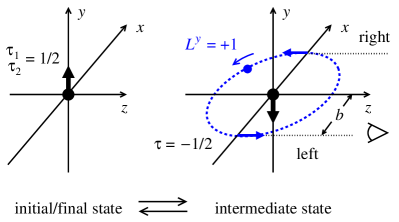
Figure 4: Quantum–mechanical picture of chiral dynamics in the peripheral transverse densities (explanation in text).

In sum, the LF formulation of chiral EFT provides a concise representation of the peripheral transverse densities, which reveals new properties (positivity, inequality) and permits a simple mechanical interpretation. The large left–right asymmetry is rooted in the spin structure of the pion–nucleon coupling and the essentially relativistic motion of pions and represents a striking chiral effect. It could be observed by extracting the peripheral transverse densities from precise measurements of the nucleon’s Dirac and Pauli form factors at low momentum transfer, using dispersion fits that respect the analytic properties Belushkin:2006qa ; see Ref. Miller:2011du for details. Similar chiral left–right asymmetries may be observed in high-energy proton–proton collisions, by selecting events in which the scattering takes place on a peripheral pion; such processes would permit much more direct tests of the effect described here.

The LF wave function representation of peripheral transverse densities can be extended to include intermediate $\Delta$ isobars and implement the proper scaling behavior in the large–$N_{c}$ limit of QCD Strikman:2010pu ; Granados:2013moa . It can also be used to compute the peripheral densities of matter and angular momentum (describing the form form factors of the energy–momentum tensor) and develop a mechanical representation of these structures. It can be applied further to the nucleon’s peripheral parton densities (generalized parton distributions) Strikman:2003gz . The LF representation has also been employed to study aspects of chiral nucleon structure (self–energies, electromagnetic couplings) without restriction to peripheral distances Ji:2009jc .

Notice: Authored by Jefferson Science Associates, LLC under U.S. DOE Contract No. DE-AC05-06OR23177. The U.S. Government retains a non–exclusive, paid–up, irrevocable, world–wide license to publish or reproduce this manuscript for U.S. Government purposes.

References

- (1) J. Gasser and H. Leutwyler, Annals Phys. 158, 142 (1984); Nucl. Phys. B 250, 465 (1985).
- (2) S. Weinberg, Phys. Lett. B 251, 288 (1990); Nucl. Phys. B 363, 3 (1991).
- (3) P. A. M. Dirac, Rev. Mod. Phys. 21, 392 (1949).
- (4) H. Leutwyler and J. Stern, Annals Phys. 112, 94 (1978).
- (5) S. J. Brodsky, H.–C. Pauli and S. S. Pinsky, Phys. Rept. 301, 299 (1998).
- (6) D. E. Soper, Phys. Rev. D 15, 1141 (1977).
- (7) M. Burkardt, Phys. Rev. D 62, 071503 (2000) [Erratum-ibid. D 66, 119903 (2002)].
- (8) M. Burkardt, Int. J. Mod. Phys. A 18, 173 (2003).
- (9) G. A. Miller, Phys. Rev. Lett. 99, 112001 (2007); Ann. Rev. Nucl. Part. Sci. 60, 1 (2010).
- (10) C. Granados and C. Weiss, in preparation (2015).
- (11) C. Granados and C. Weiss, JHEP 1401, 092 (2014).
- (12) M. Strikman and C. Weiss, Phys. Rev. C 82, 042201 (2010).
- (13) J. Gasser, M. E. Sainio and A. Svarc, Nucl. Phys. B 307, 779 (1988).
- (14) V. Bernard, N. Kaiser, J. Kambor and U.–G. Meissner, Nucl. Phys. B 388, 315 (1992).
- (15) B. Kubis and U.–G. Meissner, Nucl. Phys. A 679, 698 (2001).
- (16) T. Becher and H. Leutwyler, Eur. Phys. J. C 9, 643 (1999).
- (17) M. A. Belushkin, H.–W. Hammer and U.–G. Meissner, Phys. Rev. C 75, 035202 (2007). I. T. Lorenz, H.–W. Hammer and U.–G. Meissner, Eur. Phys. J. A 48, 151 (2012).
- (18) G. A. Miller, M. Strikman and C. Weiss, Phys. Rev. C 84, 045205 (2011).
- (19) M. Strikman and C. Weiss, Phys. Rev. D 69, 054012 (2004); Phys. Rev. D 80, 114029 (2009).
- (20) C.–R. Ji, W. Melnitchouk and A. W. Thomas, Phys. Rev. D 80, 054018 (2009); Phys. Rev. D 88, 076005 (2013). M. Burkardt, K. S. Hendricks, C.–R. Ji, W. Melnitchouk and A. W. Thomas, Phys. Rev. D 87, 056009 (2013).