Estimation after Parameter Selection: Performance Analysis and Estimation Methods

Abstract

In many practical parameter estimation problems, prescreening and parameter selection are performed prior to estimation. In this paper, we consider the problem of estimating a preselected unknown deterministic parameter chosen from a parameter set based on observations according to a predetermined selection rule, $\Psi$. The data-based parameter selection process may impact the subsequent estimation by introducing a selection bias and creating coupling between decoupled parameters. This paper introduces a post-selection mean squared error (PSMSE) criterion as a performance measure. A corresponding Cram$\acute{\text{e}}$r-Rao-type bound on the PSMSE of any $\Psi$-unbiased estimator is derived, where the $\Psi$-unbiasedness is in the Lehmann-unbiasedness sense. The post-selection maximum-likelihood (PSML) estimator is presented. It is proved that if there exists an $\Psi$-unbiased estimator that achieves the $\Psi$-Cram$\acute{\text{e}}$r-Rao bound (CRB), i.e., an $\Psi$-efficient estimator, then it is produced by the PSML estimator. In addition, iterative methods are developed for the practical implementation of the PSML estimator. Finally, the proposed $\Psi$-CRB and PSML estimator are examined in estimation after parameter selection with different distributions.

I Introduction

Statistical inference on multiple parameters often involves a preliminary data-driven parameter selection stage. In mathematical statistics literature, estimation after parameter selection refers to the problem in which estimation is performed only after a specific population, related to a specific parameter has been selected from a set of possible independent populations. The population selection is based on some predetermined data-based selection rule, $\Psi$, where $\Psi$ may not be optimal in any sense. In cognitive radio communications [1], for example, the parameters of a channel are estimated only after the channel has been identified in the white space, often thresholding on the empirical signal to noise ratio as a selection criterion. In medical diagnoses, a special test is administered only after other preliminary tests indicate that a patient may have contracted a certain disease. Other applications include multiple radar subset selection problems [2], medical experiments [3], genetic studies [4], and estimation in wireless sensor networks after sensor node selection [5].

Despite the importance of estimation after parameter selection, the impact of selection procedure on the fundamental limits of estimation performance for general parametric models is not well understood. It is known that the selection process affect the statistical properties of the subsequent estimation [6]. In particular, the bias and mean squared error (MSE) criterion are inappropriate (e.g. [7], [8]) and the conventional Cram$\acute{\text{e}}$r-Rao bound (CRB) is unsuited since it does not take the prescreening process into account. In addition, the selection may create coupling between originally decoupled parameters and it usually induces a bias, or “winner’s curse” [4], on any estimator of the selected unknown parameter. For example, for the exponential family of distributions, no unbiased estimator exists for classical estimation after selection with independent population and a single sampling stage and data-based selection rules [8, 9, 10].

I-A Summary of results

In this work, we are interested in the problem of estimation after parameter selection, i.e., estimating a subset of parameters after they are selected based on a data-based selection rule. This problem is a generalization of the classical estimation after selection problem [6], where each parameter is associated with a specific non-overlapped set of observations, named a population, and the populations are assumed to be independent. Another special case of the model considered here is the problem of estimation in the presence of nuisance parameters [11], [12]. In such a problem the parameter of interest is chosen in advance independent of data.

In order to characterize the estimation performance of the selected parameter, we introduce the post-selection MSE (PSMSE) criterion and the concept of $\Psi$-unbiasedness by using the non-Bayesian Lehmann-unbiasedness definition [13]. Then we develop the appropriate CRB-type bound on the PSMSE of any $\Psi$-unbiased estimator. In addition, we present the post-selection maximum-likelihood (PSML) estimator, which is the corresponding maximum-likelihood (ML) estimator for estimation after parameter selection problems. We show that if an $\Psi$-unbiased estimator exists that achieves the $\Psi$-CRB, it is produced by the PSML estimator. We further develop iterative methods for the practical implementation of the PSML estimator. Finally, the proposed $\Psi$-CRB and PSML estimator are examined on uniform, exponential, and Gaussian distributions with the sample mean selection (SMS) rule.

I-B Related works

The earliest works on classical estimation after selection with independent populations are by Sarkadi, Putter, and Rubinstein in [7] and [8]. These works, as well as studies that appear in mathematical statistics literature, assume random unknown parameters and show that no unbiased estimator exists for independent Gaussian populations. In mathematical statistics literature, estimation after selection with independent populations has received considerable attention over the years, where most of the work is restricted to specific parametric models, such as the Gaussian [3, 9, 14, 15], Gamma [16, 17], and uniform [18] models. Several estimation methods have been proposed to reduce the selection bias by employing various iterative methods for bias correction (e.g. [19], [20]). Shrinkage, minimax, and Bayesian techniques have also been studied [21], [22]. For cases in which an unbiased estimator exists, the U-V estimator by Robbins can be used [23]. The current paper provides a general non-Bayesian framework, i.e., where the parameters to be estimated after selection are deterministic and the underlying statistical models are general and admit general dependencies across parameters. In particular, we establish the basic theory of $\Psi$-efficiency post selection estimation that includes the fundamental limits of estimation, ways to achieve efficiency when efficient estimator exists, and practical approaches.

In the context of signal processing, the works in [24] and [25] investigate the Bayesian estimation after the detection of an unknown data region of interest. The problem of post-detection estimation, or estimation after data censoring, is considered by Chaumette, Larzabal, and Forster [26], [27], who derive a novel CRB on the conditional MSE, involving conditional Fisher information. It should be noted that in [26, 27, 24, 25], the selection rule selects the data to be used, while in our proposed model the parameter to be estimated is selected and all the data can be used for estimation. Selection and ranking are highly related approaches [6]. Detection and estimation after ranking and order statistics procedures are proposed in [28, 29] and are shown to have both practical and theoretical advantages in terms of computational complexity and performance. An empirical Bayes estimator for exponentially distributed populations is proposed in [30]. For the problem of estimation after model selection, a bootstrap method for computing standard errors and confidence intervals is considered in [31], a post-selection lasso method is developed in [32], and the CRB is derived in [33] for model order selection. However, it should be emphasized that in the case of estimation after parameter selection presented here, the measurement model is assumed to be known and there are no modeling errors. In contrast, in estimation after model selection [31], [33], the measurement model is unknown and is selected from a finite collection of competing models.

I-C Organization and notations

The remainder of the paper is organized as follows: Section II presents the mathematical model for the problem of estimation after parameter selection. The $\Psi$-unbiasedness in the Lehmann sense and the $\Psi$-CRB are derived in Section III and estimation methods are developed in Section IV, for estimation after parameter selection. Finally, the proposed $\Psi$-CRB and $\Psi$-unbiased estimators are evaluated via simulations for the linear Gaussian model in Section V. Our conclusions appear in Section VI.

In the rest of this paper, vectors are denoted by boldface lowercase letters and matrices by boldface uppercase letters. The operators $(\cdot)^{\mbox{\tiny$T$}}$ and $(\cdot)^{-1}$ denote the transpose and inverse, respectively. The vector ${\bf{e}}_{m}\in{\mathbb{R}}^{M}$ is a vector of all zeros except for a 1 at the $m$th position, $\forall m=1,\ldots,M$, and the $(m,k)$th element of the matrix ${\bf{A}}$ is denoted by $[{\bf{A}}]_{m,k}$. The notations $\delta_{m,k}$ and ${\mathbf{1}}_{A}$ denote the Kronecker delta function and the indicator function of an event $A$, respectively. The $m$th element of the gradient vector $\nabla_{\mbox{\boldmath{\scriptsize$\theta$}}}c$ is given by $\frac{\partial c}{\partial\theta_{m}}$, where ${\mbox{\boldmath$\theta$}}=[\theta_{1},\ldots,\theta_{M}]^{\mbox{\tiny$T$}}$, $c$ is an arbitrary scalar function of $\theta$, $\nabla_{\mbox{\boldmath{\scriptsize$\theta$}}}^{T}c\stackrel{{\scriptstyle\triangle}}{{=}}(\nabla_{\mbox{\boldmath{\scriptsize$\theta$}}}c)^{T}$, and $\nabla_{\mbox{\boldmath{\scriptsize$\theta$}}}^{2}c\stackrel{{\scriptstyle\triangle}}{{=}}\nabla_{\mbox{\boldmath{\scriptsize$\theta$}}}\nabla_{\mbox{\boldmath{\scriptsize$\theta$}}}^{T}c$. The notations ${\rm{E}}_{{\mbox{\boldmath{\scriptsize$\theta$}}}}[\cdot]$ and ${\rm{E}}_{{\mbox{\boldmath{\scriptsize$\theta$}}}}[\cdot|A]$ represent the expected and conditional-expected value of its argument, parameterized by a deterministic parameter $\theta$ and given event $A$.

II Problem formulation

Let $(\Omega_{\bf{x}},{\cal{F}},P_{\mbox{\boldmath{\scriptsize$\theta$}}})$ denote a probability space, where $\Omega_{\bf{x}}$ is the observation space, ${\cal{F}}$ is the $\sigma$-algebra on $\Omega_{\bf{x}}$, and $\left\{P_{\mbox{\boldmath{\scriptsize$\theta$}}}\right\}$ is a family of probability measures parametrized by the deterministic parameter vector ${\mbox{\boldmath$\theta$}}=[\theta_{1},\ldots,\theta_{M}]^{\mbox{\tiny$T$}}\in{\mathbb{R}}^{M}$. Let $\hat{{\mbox{\boldmath$\theta$}}}=[\hat{\theta}_{1},\ldots,\hat{\theta}_{M}]^{\mbox{\tiny$T$}}$ be an estimator of $\theta$, based on a random observation vector ${\bf{x}}\in\Omega_{\bf{x}}$, i.e., $\hat{{\mbox{\boldmath$\theta$}}}:\Omega_{\bf{x}}\rightarrow{\mathbb{R}}^{M}$. For each probability measure $P_{\mbox{\boldmath{\scriptsize$\theta$}}}$, the function $f({\bf{x}};{\mbox{\boldmath$\theta$}})$ denotes the corresponding probability density function (pdf) of ${\bf{x}}$. All the estimators in this paper are assumed to be in the Hilbert space of absolutely square integrable functions with respect to (w.r.t.) $P_{\mbox{\boldmath{\scriptsize$\theta$}}}$, ${\mathcal{L}}_{2}({\mbox{\boldmath$\theta$}})$.

The basic structure of the proposed model for estimation after parameter selection consists of two stages: first, a parameter $\theta_{m}$ is selected according to a predetermined data-driven selection rule, $\Psi$, and then, this parameter is estimated. In this work, we assume that the selection rule $\Psi$ is given and we focus on the estimation of the selected parameter. The proposed model is presented schematically in Fig. 1. The extension for a selection of a subset of unknown parameters, i.e., the multiparameter case, is discussed in Section III-D.

A data-based selection rule is a deterministic function $\Psi:\Omega_{\bf{x}}\rightarrow\{1,\ldots,M\}$ that selects a parameter based on the observation vector, ${\bf{x}}$. That is, if $\Psi({\bf{x}})=m$, then the estimation goal is to estimate the parameter $\theta_{m}$ based on the same observation vector ${\bf{x}}$. We assume that the deterministic sets ${\mathcal{A}}_{m}\stackrel{{\scriptstyle\triangle}}{{=}}\{{\bf{x}}:{\bf{x}}\in\Omega_{\bf{x}},\Psi({\bf{x}})=m\}$, $m=1,\ldots,M$, partition $\Omega_{\bf{x}}$. For the sake of simplicity of notation, in the following $\Psi({\bf{x}})$ is replaced by $\Psi$. By using Bayes’ rule it can be seen that the pdf of the observation conditioned on the event ${\bf{x}}\in{\mathcal{A}}_{m}$ is

$$f({\bf{x}}|\Psi=m;{\mbox{\boldmath$\theta$}})=\frac{f({\bf{x}};{\mbox{\boldmath$\theta$}})}{\Pr(\Psi=m;{\mbox{\boldmath$\theta$}})},~{}~{}~{}\forall{\bf{x}}\in{\mathcal{A}}_{m}$$ (1)

and is undefined otherwise, where $\Pr(\Psi=m;{\mbox{\boldmath$\theta$}})$ denotes the probability of this event for all $m=1,\ldots,M$.

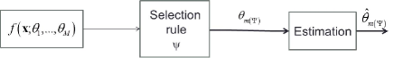
Figure 1: Schematic model of estimation after parameter selection.

A special case of the proposed model of estimation after parameter selection is estimation in the presence of additional undesired deterministic nuisance parameters [11], [12]. Here, the selection of the desired parameter is performed in advance, independently of the data, ${\bf{x}}$. Therefore, the statistical characteristics, such as CRB and bias, are not affected by the selection process and are equal to those of the multiparameter estimation, in which the nuisance parameters are estimated as well [11], [34].

A more challenging and relevant application of the proposed model is the classical estimation after selection with independent populations [7], [8], which is presented schematically in Fig. 2. In estimation after selection with independent populations, a given set of $M$ independent populations is assumed. These populations might represent, for example, a set of $M$ different communication channels. For any $m=1,\ldots,M$, it is supposed that $N_{m}\geq 1$ random observations are drawn from the $m$th population to generate the $m$th observation vector, ${\bf{y}}_{m}=[y_{m}[0],\ldots,y_{m}[N_{m}-1]]^{\mbox{\tiny$T$}}$, with the associated marginal pdf, $f_{m}({\bf{y}}_{m};\theta_{m})$, in which $\theta_{m}\in{\mathbb{R}}$ denotes the unknown parameter related to the $m$th population. In this case, the observation vector is given by ${\bf{x}}=[{\bf{y}}_{1}^{\mbox{\tiny$T$}},\ldots,{\bf{y}}_{M}^{\mbox{\tiny$T$}}]^{\mbox{\tiny$T$}}$, the joint pdf of the $M$ populations is $f({\bf{x}};{\mbox{\boldmath$\theta$}})=\prod_{m=1}^{M}f_{m}({\bf{y}}_{m};\theta_{m})$, and the selection of a parameter $\theta_{m}$ is equivalent to the selection of the $m$th population or channel.

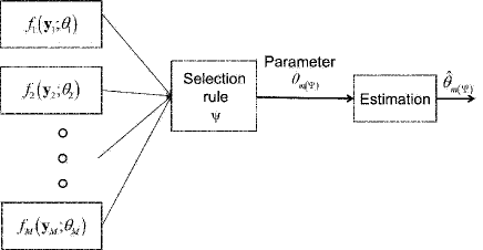
Figure 2: Schematic model of classical estimation after selection with independent populations.

In this work, we are interested in the parameter estimation of the unknown deterministic vector $\theta$, where only estimation errors of the selected parameter are taken into consideration and the selection rule is predetermined. Therefore, for a given selection rule, $\Psi$, we use the following post-selection squared-error (PSSE) cost [3, 6, 7, 35]:

$$C^{(\Psi)}(\hat{{\mbox{\boldmath$\theta$}}},{\mbox{\boldmath$\theta$}})\stackrel{{\scriptstyle\triangle}}{{=}}\sum_{m=1}^{M}(\hat{\theta}_{m}-\theta_{m})^{2}{\mathbf{1}}_{\{\Psi=m\}}.$$ (2)

The corresponding PSMSE is given by

$${\rm{E}}_{{\mbox{\boldmath{\scriptsize$\theta$}}}}\left[C^{(\Psi)}(\hat{{\mbox{\boldmath$\theta$}}},{\mbox{\boldmath$\theta$}})\right]={\rm{E}}_{{\mbox{\boldmath{\scriptsize$\theta$}}}}\left[\sum_{m=1}^{M}(\hat{\theta}_{m}-\theta_{m})^{2}{\mathbf{1}}_{\{\Psi=m\}}\right]$$

$$=\sum_{m=1}^{M}\Pr(\Psi=m;{\mbox{\boldmath$\theta$}}){\rm{E}}_{{\mbox{\boldmath{\scriptsize$\theta$}}}}\left[(\hat{\theta}_{m}-\theta_{m})^{2}|\Psi=m\right],$$ (3)

where (II) is calculated by using the densities $f({\bf{x}};{\mbox{\boldmath$\theta$}})$ and $f({\bf{x}}|\Psi=m;{\mbox{\boldmath$\theta$}})$ for the first and the second terms, respectively. The component-wise PSMSE of a specific parameter is defined as

$${\rm{E}}_{{\mbox{\boldmath{\scriptsize$\theta$}}}}\left[\left.(\hat{\theta}_{m}-\theta_{m})^{2}\right|\Psi=m\right],~{}~{}~{}m=1,\ldots,M.$$

The use of the indicator functions implies that the PSMSE may be equal for two estimators that have different values with a nonzero probability, i.e., outside the subset indicated by these indicators. In fact, $\hat{\theta}_{m}$ affects the PSMSE only for observations ${\bf{x}}\in{\mathcal{A}}_{m}$.

In the mathematical statistics literature, the unknown parameter for estimation after selection with independent populations is usually defined as $\sum_{m=1}^{M}\theta_{m}{\mathbf{1}}_{\{\Psi=m\}}$, which has both random and deterministic components. In this work, we are interested in the estimation of the deterministic parameter $\theta$. The notion of non-Bayesian estimation allows the derivation of the corresponding CRB-type lower bound and non-Bayesian estimation methods.

III The Cram$\acute{\text{e}}$r-Rao-type bound for estimation after parameter selection

The CRB (e.g. [11], [36]) provides a lower bound on the MSE of any mean-unbiased estimator and is used as a benchmark to study the optimality of practical parametric estimators. In this section, a CRB-type lower bound for estimation after parameter selection is derived. The proposed bound is a lower bound on the PSMSE of any Lehmann unbiased estimator, as described in the following.

III-A $\Psi$-unbiasedness

The mean-unbiasedness constraint is commonly used in non-Bayesian parameter estimation [11]. However, a mean-unbiased estimator is inappropriate for estimation after parameter selection problems, since we are interested only in errors of the selected parameter (See, e.g. [6], [10]). Lehmann [13] proposed a generalization of the unbiasedness concept, which is based on the considered cost function. In this section, the general Lehmann unbiasedness is used to define the unbiasedness for estimation after parameter selection problems.

Definition 1

The estimator $\hat{{\mbox{\boldmath$\theta$}}}$ is said to be an unbiased estimator of $\theta$ in the Lehmann sense [13] w.r.t. the scalar nonnegative cost function $C(\hat{{\mbox{\boldmath$\theta$}}},{\mbox{\boldmath$\theta$}})$ if

$${\rm{E}}_{{\mbox{\boldmath{\scriptsize$\theta$}}}}\left[C(\hat{{\mbox{\boldmath$\theta$}}},{\mbox{\boldmath$\eta$}})\right]\geq{\rm{E}}_{{\mbox{\boldmath{\scriptsize$\theta$}}}}\left[C(\hat{{\mbox{\boldmath$\theta$}}},{\mbox{\boldmath$\theta$}})\right],~{}~{}~{}\forall{\mbox{\boldmath$\eta$}},{\mbox{\boldmath$\theta$}}\in\Omega_{\mbox{\boldmath{\scriptsize$\theta$}}},$$ (4)

where $\Omega_{\mbox{\boldmath{\scriptsize$\theta$}}}$ is the parameter space.

The Lehmann unbiasedness definition implies that an estimator is unbiased if, on average, it is “closer” to the true parameter $\theta$ than to any other value in the parameter space. The measure of “closeness” between the estimator and the parameter is the mean of the cost function, $C(\hat{{\mbox{\boldmath$\theta$}}},{\mbox{\boldmath$\theta$}})$. For example, it is shown in [13] that under the squared-error cost function the Lehmann unbiasedness in (4) is reduced to the conventional mean-unbiasedness, ${\rm{E}}_{{\mbox{\boldmath{\scriptsize$\theta$}}}}[\hat{{\mbox{\boldmath$\theta$}}}]={\mbox{\boldmath$\theta$}}$, $\forall{\mbox{\boldmath$\theta$}}\in\Omega_{\mbox{\boldmath{\scriptsize$\theta$}}}$. Additional examples for Lehmann unbiasedness with different cost functions can be found, for example, in [13], [37], and [38]. The following proposition describes the Lehmann unbiasedness for the estimation after parameter selection, named $\Psi$-unbiasedness.

Proposition 1

An estimator $\hat{{\mbox{\boldmath$\theta$}}}:\Omega_{\bf{x}}\rightarrow{\mathbf{R}}^{M}$ is an unbiased estimator of ${\mbox{\boldmath$\theta$}}\in{\mathbf{R}}^{M}$ in the Lehmann sense w.r.t. the PSSE cost and the selection rule $\Psi$ iff

$${\rm{E}}_{{\mbox{\boldmath{\scriptsize$\theta$}}}}\left[(\hat{\theta}_{m}-\theta_{m}){\mathbf{1}}_{\{\Psi=m\}}\right]=0,~{}\forall m=1,\ldots,M,~{}\forall{\mbox{\boldmath$\theta$}}\in{\mathbb{R}}^{M},$$ (5)

or, equivalently,

$${\rm{E}}_{{\mbox{\boldmath{\scriptsize$\theta$}}}}\left[\hat{\theta}_{m}-\theta_{m}|\Psi=m\right]=0,~{}~{}~{}\forall{\mbox{\boldmath$\theta$}}\in{\mathbb{R}}^{M}$$ (6)

for all $m=1,\ldots,M$ such that $\Pr(\Psi=m;{\mbox{\boldmath$\theta$}})\neq 0$.

Proof: The proof appears in Appendix A.

It can be seen that the Lehmann unbiasedness definition in (5) and (6) is a function of the given selection rule. Therefore, in the following, an estimator $\hat{{\mbox{\boldmath$\theta$}}}$ is said to be an $\Psi$-unbiased estimate of $\theta$ for the selection rule $\Psi$, if (5) (or, equivalently, (6)) is satisfied. The concept of risk-unbiased in the Lehmann sense for the classical estimation after selection with independent populations has been discussed in the literature for the random parameter $\sum_{m=1}^{M}\theta_{m}{\mathbf{1}}_{\{\Psi=m\}}$ and various cost functions (e.g. [39] and [40]).

III-B The $\Psi$-CRB

Obtaining an estimator with the minimum PSMSE among all $\Psi$-unbiased estimators is usually not tractable and a uniform $\Psi$-unbiased minimum PSMSE estimator may not exist [7]. Thus, lower bounds on the performance of any $\Psi$-unbiased estimator are useful for performance analysis and system design. In the following, a new version of the CRB for estimation after parameter selection is derived. It should be noticed that, in general, the minimum PSMSE estimator is not unique since only the estimation errors of the selected parameter are taken into consideration.

Let us define the following post-selection Fisher information matrix (PSFIM) of the $m$th component:

$${\bf{J}}_{m}({\mbox{\boldmath$\theta$}},\Psi) \stackrel{{\scriptstyle\triangle}}{{=}} {\rm{E}}_{{\mbox{\boldmath{\scriptsize$\theta$}}}}\left[\nabla_{\mbox{\boldmath{\scriptsize$\theta$}}}\log f({\bf{x}}|\Psi=m;{\mbox{\boldmath$\theta$}})\right.$$ (7)

$$\left.\left.\times\nabla_{\mbox{\boldmath{\scriptsize$\theta$}}}^{T}\log f({\bf{x}}|\Psi=m;{\mbox{\boldmath$\theta$}})\right|\Psi=m\right],$$

for all $m=1,\ldots,M$. In addition, we define the following conditions that are a modified form of the well-known CRB regularity conditions (e.g. [36], pp. 440-441).

1. The post-selection likelihood gradient vector, $\nabla_{\mbox{\boldmath{\scriptsize$\theta$}}}\log f({\bf{x}}|\Psi=m;{\mbox{\boldmath$\theta$}})$, exists and is finite for any ${\mbox{\boldmath$\theta$}}\in{\mathbb{R}}^{M}$, ${\bf{x}}\in{\mathcal{A}}_{m}$, and $\forall m=1,\ldots,M$. That is, we assume that the $m$th PSFIM, ${\bf{J}}_{m}({\mbox{\boldmath$\theta$}},\Psi)$, is a well-defined, nonsingular, and nonzero matrix for any ${\mbox{\boldmath$\theta$}}\in{\mathbb{R}}^{M}$ and $\forall m=1,\ldots,M$.

2. The operations of integration w.r.t. ${\bf{x}}$ and differentiation w.r.t. $\theta$ can be interchanged as follows:

   $$\int_{{\mathcal{A}}_{m}}\nabla_{\mbox{\boldmath{\scriptsize$\theta$}}}\left(g({\bf{x}},{\mbox{\boldmath$\theta$}})f({\bf{x}}|\Psi=m;{\mbox{\boldmath$\theta$}})\right){\,\mathrm{d}}{\bf{x}}\hskip 56.9055pt$$

   $$=\nabla_{\mbox{\boldmath{\scriptsize$\theta$}}}{\rm{E}}_{{\mbox{\boldmath{\scriptsize$\theta$}}}}\left[g({\bf{x}},{\mbox{\boldmath$\theta$}})|\Psi=m\right],$$ (8)

   for any ${\mbox{\boldmath$\theta$}}\in{\mathbb{R}}^{M}$ and for any differentiable and measurable function $g({\bf{x}},{\mbox{\boldmath$\theta$}})$.

Theorem 1

($\Psi$-CRB) Let the regularity conditions C.1-C.2 be satisfied and $\hat{{\mbox{\boldmath$\theta$}}}$ be an $\Psi$-unbiased estimator of ${\mbox{\boldmath$\theta$}}\in{\mathbf{R}}^{M}$ for a given selection rule, $\Psi$, with a finite second moment. Then, the PSMSE is bounded by the following Cram$\acute{\text{e}}$r-Rao-type lower bound:

$${\rm{E}}_{{\mbox{\boldmath{\scriptsize$\theta$}}}}\left[C^{(\Psi)}(\hat{{\mbox{\boldmath$\theta$}}},{\mbox{\boldmath$\theta$}})\right]\geq B^{(\Psi)}({\mbox{\boldmath$\theta$}}),$$ (9)

where

$$B^{(\Psi)}({\mbox{\boldmath$\theta$}}) \stackrel{{\scriptstyle\triangle}}{{=}} \sum_{m=1}^{M}\Pr(\Psi=m;{\mbox{\boldmath$\theta$}})\left[{\bf{J}}_{m}^{-1}({\mbox{\boldmath$\theta$}},\Psi)\right]_{m,m},$$ (10)

and ${\bf{J}}_{m}({\mbox{\boldmath$\theta$}},\Psi)$ is the PSFIM defined in (7). Furthermore, the component-wise $\Psi$-CRB on the PSMSE of a specific parameter is given by

$${\rm{E}}_{{\mbox{\boldmath{\scriptsize$\theta$}}}}\left[(\hat{\theta}_{m}-\theta_{m})^{2}|\Psi=m\right]\geq\left[{\bf{J}}_{m}^{-1}({\mbox{\boldmath$\theta$}},\Psi)\right]_{m,m},$$ (11)

for all $m=1,\ldots,M$. The equality holds in (9) and (11) iff there exist functions $h_{m}({\mbox{\boldmath$\theta$}})$, $m=1,\ldots,M$, such that

$$\sum_{l=1}^{M}\frac{\partial\log f({\bf{x}}|\Psi=m;{\mbox{\boldmath$\theta$}})}{\partial\theta_{l}}\left[{\bf{J}}_{m}^{-1}({\mbox{\boldmath$\theta$}},\Psi)\right]_{l,m}=\hskip 28.45274pt$$

$$h_{m}({\mbox{\boldmath$\theta$}})(\hat{\theta}_{m}-\theta_{m}),~{}~{}~{}\forall m=1,\ldots,M$$ (12)

almost surely (a.s.) ${\bf{x}}\in{\mathcal{A}}_{m}$.

Proof:

According to the Cauchy-Schwarz inequality:

$${\rm{E}}_{{\mbox{\boldmath{\scriptsize$\theta$}}}}\left[\left.\eta^{2}({\bf{x}},{\mbox{\boldmath$\theta$}})\right|\Psi=m\right]\geq\frac{{\rm{E}}_{{\mbox{\boldmath{\scriptsize$\theta$}}}}^{2}\left[\left.\eta({\bf{x}},{\mbox{\boldmath$\theta$}})d({\bf{x}},{\mbox{\boldmath$\theta$}})\right|\Psi=m\right]}{{\rm{E}}_{{\mbox{\boldmath{\scriptsize$\theta$}}}}\left[\left.d^{2}({\bf{x}},{\mbox{\boldmath$\theta$}})\right|\Psi=m\right]},$$ (13)

for any measurable functions $\eta({\bf{x}},{\mbox{\boldmath$\theta$}})$ and $h({\bf{x}},{\mbox{\boldmath$\theta$}})$ with finite second moments. By substituting $\eta({\bf{x}},{\mbox{\boldmath$\theta$}})=\hat{\theta}_{m}-\theta_{m}$ and

$$d({\bf{x}},{\mbox{\boldmath$\theta$}})=\sum_{l=1}^{M}\frac{\partial\log f({\bf{x}}|\Psi=m;{\mbox{\boldmath$\theta$}})}{\partial\theta_{l}}\left[{\bf{J}}_{m}^{-1}({\mbox{\boldmath$\theta$}},\Psi)\right]_{l,m}$$

in (13) and under Condition C.1, one obtains

$${\rm{E}}_{{\mbox{\boldmath{\scriptsize$\theta$}}}}\left[\left.(\hat{\theta}_{m}-\theta_{m})^{2}\right|\Psi=m\right]\geq\hskip 106.69783pt$$

$$\frac{\left(\sum\limits_{l=1}^{M}a_{l,m}({\mbox{\boldmath$\theta$}})\left[{\bf{J}}_{m}^{-1}({\mbox{\boldmath$\theta$}},\Psi)\right]_{l,m}\right)^{2}}{\sum\limits_{l=1}^{M}\sum\limits_{k=1}^{M}\left[{\bf{J}}_{m}({\mbox{\boldmath$\theta$}},\Psi)\right]_{k,l}\left[{\bf{J}}_{m}^{-1}({\mbox{\boldmath$\theta$}},\Psi)\right]_{l,m}\left[{\bf{J}}_{m}^{-1}({\mbox{\boldmath$\theta$}},\Psi)\right]_{m,k}},$$ (14)

for any estimator with ${\rm{E}}_{{\mbox{\boldmath{\scriptsize$\theta$}}}}\left[\left.(\hat{\theta}_{m}-\theta_{m})^{2}\right|\Psi=m\right]<\infty$ and a nonsingular PSFIM, where

$$a_{l,m}({\mbox{\boldmath$\theta$}})\stackrel{{\scriptstyle\triangle}}{{=}}{\rm{E}}_{{\mbox{\boldmath{\scriptsize$\theta$}}}}\left[\left.\frac{\partial\log f({\bf{x}}|\Psi=m;{\mbox{\boldmath$\theta$}})}{\partial\theta_{l}}(\hat{\theta}_{m}-\theta_{m})\right|\Psi=m\right],$$

for all $m,l=1,\ldots,M$. According to the Cauchy-Schwarz conditions, the equality in (III-B) holds iff (1) is satisfied for $m\in\{1,\ldots,M\}$. By using integration by parts and assuming Condition C.2, it can be verified that

$$a_{l,m}({\mbox{\boldmath$\theta$}})=\frac{\partial}{\partial\theta_{l}}{\rm{E}}_{{\mbox{\boldmath{\scriptsize$\theta$}}}}\left[\left.(\hat{\theta}_{m}-\theta_{m})\right|\Psi=m\right]+\delta_{l,m}=\delta_{l,m},$$ (15)

for all $m,l=1,\ldots,M$, where the last equality is obtained by using the $\Psi$-unbiasedness conditions from (6). In addition, it can be verified that

$${\sum\limits_{l=1}^{M}\sum\limits_{k=1}^{M}\left[{\bf{J}}_{m}({\mbox{\boldmath$\theta$}},\Psi)\right]_{k,l}\left[{\bf{J}}_{m}^{-1}({\mbox{\boldmath$\theta$}},\Psi)\right]_{l,m}\left[{\bf{J}}_{m}^{-1}({\mbox{\boldmath$\theta$}},\Psi)\right]_{m,k}}$$

$$=\left[{\bf{J}}_{m}^{-1}({\mbox{\boldmath$\theta$}},\Psi)\right]_{m,m}.\hskip 85.35826pt$$ (16)

By substituting (15) and (III-B) in (III-B), we obtain the component-wise $\Psi$-CRBs on the PSMSE in (11). Then, by multiplying (11) by $\Pr(\Psi=m;{\mbox{\boldmath$\theta$}})$ and taking the sum of over $m=1,\ldots,M$, we obtain the $\Psi$-CRB in (9). Furthermore, the equality condition in (1) stems from the equality conditions of (III-B). ∎

The following Lemma presents two alternative formulations of the PSFIM that are based on the (unconditional) likelihood function and the probability of selection, instead of the conditional likelihood used in (7). These formulations can be more tractable for further estimation and sampling procedures.

Lemma 1

Assuming that Conditions C.1-C.2 are satisfied, the second derivative w.r.t. $\theta$ of $f({\bf{x}}|\Psi=m;{\mbox{\boldmath$\theta$}})$ exists and is bounded and continuous $\forall{\bf{x}}\in{\mathcal{A}}_{m}$, and the integral $\int_{{\mathcal{A}}_{m}}f({\bf{x}}|\Psi=m;{\mbox{\boldmath$\theta$}}){\,\mathrm{d}}{\bf{x}}$ is twice differentiable under the integral sign for all $m=1,\ldots,M$, ${\mbox{\boldmath$\theta$}}\in{\mathbb{R}}^{M}$. Then, the $m$th PSFIM in (7) satisfies

$${\bf{J}}_{m}({\mbox{\boldmath$\theta$}},\Psi)={\rm{E}}_{{\mbox{\boldmath{\scriptsize$\theta$}}}}\left[\left.\nabla_{\mbox{\boldmath{\scriptsize$\theta$}}}\log f({\bf{x}};{\mbox{\boldmath$\theta$}})\nabla_{\mbox{\boldmath{\scriptsize$\theta$}}}^{T}\log f({\bf{x}};{\mbox{\boldmath$\theta$}})\right|\Psi=m\right]$$

$$-\nabla_{\mbox{\boldmath{\scriptsize$\theta$}}}\log\Pr(\Psi=m;{\mbox{\boldmath$\theta$}})\nabla_{\mbox{\boldmath{\scriptsize$\theta$}}}^{T}\log\Pr(\Psi=m;{\mbox{\boldmath$\theta$}})$$ (17)

and

$${\bf{J}}_{m}({\mbox{\boldmath$\theta$}},\Psi)= - {\rm{E}}_{{\mbox{\boldmath{\scriptsize$\theta$}}}}\left[\left.\nabla_{\mbox{\boldmath{\scriptsize$\theta$}}}^{2}\log f({\bf{x}};{\mbox{\boldmath$\theta$}})\right|\Psi=m\right]$$ (18)

$$+ \nabla_{\mbox{\boldmath{\scriptsize$\theta$}}}^{2}\log\Pr(\Psi=m;{\mbox{\boldmath$\theta$}}),$$

for all $m=1,\ldots,M$, ${\mbox{\boldmath$\theta$}}\in{\mathbb{R}}^{M}$, and for any selection rule $\Psi$.

Proof: The proof appears in Appendix B.

Similar to the $\Psi$-CRB from Theorem 1, by using the Cauchy-Schwarz inequality and the $\Psi$-unbiasedness we can obtain various non-Bayesian bounds on the PSMSE These bounds are modifications of various non-Bayesian bounds, such as the biased CRB and Barankin-type bounds [41, 42, 43].

III-C Special cases

In this section, we demonstrate the proposed $\Psi$-CRB and $\Psi$-unbiasedness for different cases.

III-C1 Randomized selection rule

The randomized, coin-flipping selection rule satisfies $\Pr(\Psi_{\text{rand}}=m;{\mbox{\boldmath$\theta$}})=p_{m}$, for all $m=1,\ldots,M$, where $\{p_{m}\}\in[0,1]^{M}$ are independent of ${\bf{x}}$. Therefore, the $\Psi$-unbiasedness from (5) in this case is given by

$${\rm{E}}_{{\mbox{\boldmath{\scriptsize$\theta$}}}}\left[\hat{\theta}_{m}-\theta_{m}\right]=0,~{}~{}~{}\forall{\mbox{\boldmath$\theta$}}\in{\mathbb{R}}^{M},$$ (19)

for all $m=1,\ldots,M$ with $p_{m}\neq 0$. The $\Psi$-unbiasedness in (19) is the classical mean-unbiasedness definition. In this case, the $\Psi$-CRB from (10) is reduced to

$$B^{(\Psi_{\text{rand}})}({\mbox{\boldmath$\theta$}})=\sum_{m=1}^{M}p_{m}\left[{\bf{B}}({\mbox{\boldmath$\theta$}})\right]_{m,m},$$ (20)

where ${\bf{B}}({\mbox{\boldmath$\theta$}})={\bf{J}}^{-1}\left({\mbox{\boldmath$\theta$}}\right)$ is the conventional CRB. Thus, the proposed $\Psi$-CRB for the randomized selection rule, $\Psi_{\text{rand}}$, is equal to a weighted sum of the diagonal elements of the classical CRB, ${\bf{B}}({\mbox{\boldmath$\theta$}})$, for estimating $\theta$ without a selection stage. In particular, for $p_{m}=\delta_{m,m^{\prime}}$, where $\theta_{m^{\prime}}$ is the desired parameter, we obtained an estimation problem in the presence of nuisance parameters, i.e., where the selection of the “parameter of interest” $\theta_{m^{\prime}}$ is performed in advance. It is easy to verify that in this case the $\Psi$-CRB and $\Psi$-unbiasedness are reduced to their classical, marginal versions. This result coincide with the literature on non-Bayesian nuisance parameter estimation (e.g. [11] and [34]).

III-C2 Parameter coupling

For conventional parameter estimation with a diagonal FIM, where the FIM is defined as

$${\bf{J}}({\mbox{\boldmath$\theta$}})\stackrel{{\scriptstyle\triangle}}{{=}}{\rm{E}}_{{\mbox{\boldmath{\scriptsize$\theta$}}}}\left[\nabla_{\mbox{\boldmath{\scriptsize$\theta$}}}\log f({\bf{x}};{\mbox{\boldmath$\theta$}})\nabla_{\mbox{\boldmath{\scriptsize$\theta$}}}^{T}\log f({\bf{x}};{\mbox{\boldmath$\theta$}})\right],$$ (21)

the unknown parameters are decoupled from each other; that is, knowledge of one parameter does not affect the accuracy in the estimation of the others. This situation occurs, for example, for classical estimation after selection with independent populations, in which $f({\bf{x}};{\mbox{\boldmath$\theta$}})=\prod_{m=1}^{M}f_{m}({\bf{y}}_{m};\theta_{m})$. However, it should be noted that the PSFIMs are not necessarily diagonal for diagonal FIM cases, since the selection step may create dependency and coupling between the parameters over the different populations. For example, by using the form of the PSFIM in (18), it can be seen that the matrix $\nabla_{\mbox{\boldmath{\scriptsize$\theta$}}}^{2}\log\Pr(\Psi=m;{\mbox{\boldmath$\theta$}})$ may be a nondiagonal matrix for a data-dependent selection rule.

III-C3 Biased $\Psi$-CRB

Similar to the proof of Theorem 1, it can be shown that under regularity conditions C.1-C.2 the PSMSE is bounded by the following biased $\Psi$-CRB:

$${\rm{E}}_{{\mbox{\boldmath{\scriptsize$\theta$}}}}\left[C^{(\Psi)}(\hat{{\mbox{\boldmath$\theta$}}},{\mbox{\boldmath$\theta$}})\right]\geq\sum_{m=1}^{M}\Pr(\Psi=m;{\mbox{\boldmath$\theta$}})\hskip 71.13188pt$$

$$\times\left(\nabla_{\mbox{\boldmath{\scriptsize$\theta$}}}b_{m}({\mbox{\boldmath$\theta$}})+{\bf{e}}_{m}\right)^{T}\left[{\bf{J}}_{m}^{-1}({\mbox{\boldmath$\theta$}},\Psi)\right]\left(\nabla_{\mbox{\boldmath{\scriptsize$\theta$}}}b_{m}({\mbox{\boldmath$\theta$}})+{\bf{e}}_{m}\right),$$ (22)

for any $\Psi$-biased estimator, $\hat{{\mbox{\boldmath$\theta$}}}$, with the biases

$$b_{m}({\mbox{\boldmath$\theta$}})={\rm{E}}_{{\mbox{\boldmath{\scriptsize$\theta$}}}}\left[\hat{\theta}_{m}-\theta_{m}|\Psi=m\right],~{}m=1,\ldots,M,$$

and a finite second moment.

III-D Estimation after parameter subset selection

In many problems, we are interested in selecting a subset of parameters and then, estimating the parameters of the selected subset [44, 45]. This subset may be of random size, with/without overlapping between the subspaces. The selection rule is $\Psi:\Omega_{\bf{x}}\rightarrow\{\Psi_{1},\ldots,\Psi_{L}\}$, where $\{\Psi_{1},\ldots,\Psi_{L}\}$ is a finite covering of the set $\{1,\ldots,M\}$, i.e., it is a division of $\{1,\ldots,M\}$ as a union of possibly-overlapping non-empty $L$ subsets, such as the power set. In this case, the PSSE cost function from (2) is replaced by

$$C^{(\Psi)}(\hat{{\mbox{\boldmath$\theta$}}},{\mbox{\boldmath$\theta$}})\stackrel{{\scriptstyle\triangle}}{{=}}\sum_{m=1}^{M}(\hat{\theta}_{m}-\theta_{m})^{2}{\mathbf{1}}_{\{m\in\Psi\}}$$

and the corresponding PSMSE is:

$${\rm{E}}_{{\mbox{\boldmath{\scriptsize$\theta$}}}}\left[C^{(\Psi)}(\hat{{\mbox{\boldmath$\theta$}}},{\mbox{\boldmath$\theta$}})\right] = \sum_{l=1}^{L}\Pr(\Psi=\Psi_{l};{\mbox{\boldmath$\theta$}})$$

$$\times\sum_{m=1,m\in\Psi_{l}}^{M}{\rm{E}}_{{\mbox{\boldmath{\scriptsize$\theta$}}}}\left[(\hat{\theta}_{m}-\theta_{m})^{2}|\Psi=\Psi_{l}\right].$$

Similar to Proposition 1 and Theorem 1, the $\Psi$-unbiasedness and $\Psi$-CRB for subset selection are, respectively, given by

$${\rm{E}}_{{\mbox{\boldmath{\scriptsize$\theta$}}}}\left[\left.\hat{\theta}_{m}-\theta_{m}\right|\Psi=\Psi_{l}\right]=0,~{}\begin{array}[]{l}\forall m=1,\ldots,M,~{}m\in\Psi_{l}\\ \forall l=l=1,\ldots,L\end{array}$$ (25)

for any ${\mbox{\boldmath$\theta$}}\in{\mathbb{R}}^{M}$ and

$${\rm{E}}_{{\mbox{\boldmath{\scriptsize$\theta$}}}}\left[C^{(\Psi)}(\hat{{\mbox{\boldmath$\theta$}}},{\mbox{\boldmath$\theta$}})\right]\geq B^{(\Psi)}({\mbox{\boldmath$\theta$}}),$$

where

$$B^{(\Psi)}({\mbox{\boldmath$\theta$}})\stackrel{{\scriptstyle\triangle}}{{=}}\sum_{l=1}^{L}\Pr(\Psi=\Psi_{l};{\mbox{\boldmath$\theta$}})\sum_{m=1,m\in\Psi_{l}}^{M}\left[{\bf{J}}_{l}^{-1}({\mbox{\boldmath$\theta$}},\Psi)\right]_{m,m}$$ (26)

and

$${\bf{J}}_{l}({\mbox{\boldmath$\theta$}},\Psi) \stackrel{{\scriptstyle\triangle}}{{=}} {\rm{E}}_{{\mbox{\boldmath{\scriptsize$\theta$}}}}\left[\nabla_{\mbox{\boldmath{\scriptsize$\theta$}}}\log f({\bf{x}}|\Psi=\Psi_{l};{\mbox{\boldmath$\theta$}})\right.$$

$$\left.\left.\times\nabla_{\mbox{\boldmath{\scriptsize$\theta$}}}^{T}\log f({\bf{x}}|\Psi=\Psi_{l};{\mbox{\boldmath$\theta$}})\right|\Psi=\Psi_{l}\right].$$

for all $l=1,\ldots,L$ is the PSFIM for this case.

If the selection rule selects all the $M$ parameters, then, the PSMSE is equal to the MSE and we obtain the conventional parameter estimation problem, mean-unbiasedness, and the well known CRB. Another special case of estimation after parameter subset selection is the classical estimation after selection model with independent populations, where the pdf of each single population is a function of multiple unknown parameters. For this nonoverlapped case, we can also obtain a matrix-form of the $\Psi$-CRB from (26) by using the matrix form of the Cauchy-Schwarz inequality and the vector $\Psi$-unbiasedness from (25).

III-E Estimation after data censoring

A related problem is the estimation after data censoring, which is obtained from the aforementioned model by assuming a selection rule that restricts the set of observations available for parameter estimation. In this case, we use the observations only if $\Psi=1$, and we remove them otherwise. Similar to the derivation of the $\Psi$-CRB in Theorem 1, the following matrix-form $\Psi$-CRB is obtained for this case:

$${\rm{E}}_{{\mbox{\boldmath{\scriptsize$\theta$}}}}\left[(\hat{{\mbox{\boldmath$\theta$}}}-{\mbox{\boldmath$\theta$}})(\hat{{\mbox{\boldmath$\theta$}}}-{\mbox{\boldmath$\theta$}})^{T}|\Psi=1\right]\geq{\bf{J}}_{c}^{-1}({\mbox{\boldmath$\theta$}},\Psi),$$ (27)

where

$${\bf{J}}_{c}({\mbox{\boldmath$\theta$}},\Psi) \stackrel{{\scriptstyle\triangle}}{{=}} {\rm{E}}_{{\mbox{\boldmath{\scriptsize$\theta$}}}}\left[\left.\nabla_{\mbox{\boldmath{\scriptsize$\theta$}}}\log f({\bf{x}}|\Psi=1;{\mbox{\boldmath$\theta$}})\right.\right.$$ (28)

$$\left.\left.\times\nabla_{\mbox{\boldmath{\scriptsize$\theta$}}}^{T}\log f({\bf{x}}|\Psi=1;{\mbox{\boldmath$\theta$}})\right|\Psi=1\right].$$

The bound in (27) coincides with the conditional CRB derived in [26] for estimation after binary detection, i.e., when a binary detection step is performed before the estimation of the parameters. This observation remains valid for any non-Bayesian bound on the PSMSE, which can be derived by using the Cauchy-Schwarz inequality and the $\Psi$-unbiasedness, in a similar way to the derivations in [26], [43]. However, it should be noted that in estimation after data censoring, the selection rule selects the data, while in our model the parameter to be estimated has been selected.

IV Post-selection estimation

IV-A The PSML estimator

For general parameter estimation, the commonly used ML estimator is defined as

$$\hat{{\mbox{\boldmath$\theta$}}}^{({\mbox{\tiny ML}})}=\arg\max_{\mbox{\boldmath{\scriptsize$\theta$}}}\log f({\bf{x}};{\mbox{\boldmath$\theta$}}).$$ (29)

It is well known that the ML estimator is inappropriate for estimation after parameter selection since it does not take into account the prescreening process [7], [8]. Inspired by Theorem 1, we define the PSML estimator as:

$$\hat{{\mbox{\boldmath$\theta$}}}^{({\mbox{\tiny PSML}})} = \arg\max_{\mbox{\boldmath{\scriptsize$\theta$}}}\left\{\sum_{m=1}^{M}\log f({\bf{x}}|\Psi=m;{\mbox{\boldmath$\theta$}}){\mathbf{1}}_{\{{\bf{x}}\in{\mathcal{A}}_{m}\}}\right\}$$ (30)

$$= \arg\max_{\mbox{\boldmath{\scriptsize$\theta$}}}\left\{\log f({\bf{x}};{\mbox{\boldmath$\theta$}})\right.$$

$$-\left.\sum_{m=1}^{M}\log\Pr(\Psi=m;{\mbox{\boldmath$\theta$}}){\mathbf{1}}_{\{{\bf{x}}\in{\mathcal{A}}_{m}\}}\right\},$$

where the last equality is obtained by using (1). We propose using the PSML estimator instead of the ML estimator for estimation after parameter selection problems. The PSML estimator can be interpreted as the “penalized ML estimator” [36], where the penalty term in this case is $-\sum_{m=1}^{M}\log\Pr(\Psi=m;{\mbox{\boldmath$\theta$}}){\mathbf{1}}_{\{{\bf{x}}\in{\mathcal{A}}_{m}\}}$. However, since the penalty term is not a probability density w.r.t. $\theta$, (30) does not have a Bayesian interpretation. It can be seen that if the selection probability, $\Pr(\Psi=m;{\mbox{\boldmath$\theta$}})$, is not a function of $\theta$, then the PSML estimator coincides with the ML estimator. This situation occurs, for example, for a randomized selection rule and for estimation in the presence of nuisance parameters. Under suitable regularity conditions, such as differentiability, the PSML estimator is a solution to the following score equation

$$\sum_{m=1}^{M}\nabla_{\mbox{\boldmath{\scriptsize$\theta$}}}\log f({\bf{x}}|\Psi=m;{\mbox{\boldmath$\theta$}}){\mathbf{1}}_{\{{\bf{x}}\in{\mathcal{A}}_{m}\}}={\bf{0}}.$$ (31)

The $\Psi$-efficient estimator is defined as follows.

Definition 2

An estimator is said to be an $\Psi$-efficient estimator of $\theta$ if it is an $\Psi$-unbiased estimator that achieves the $\Psi$-CRB.

It should be noticed that the requirement for equality condition in (1), i.e., for the $\Psi$-CRB achievability, is relevant only in the subspace ${\mathcal{A}}_{m}$ and the estimation errors outside this region can have arbitrary values. Thus, the estimator which satisfies the equality condition in (1), if exists, is not unique, since by changing this estimator outside the subset ${\mathcal{A}}_{m}$ we obtain a new estimator that attained (1). In particular, the $\Psi$-efficient estimator is not unique. The following theorem describes the relations between the PSML and the $\Psi$-efficient estimators.

Theorem 2

Assume that the regularity conditions C.1-C.2 are satisfied and that $\hat{{\mbox{\boldmath$\theta$}}}^{(\Psi{\text{-eff}})}$ is an $\Psi$-efficient estimator, as defined in Definition 2. Then,

$$\hat{\theta}_{m}^{(\Psi{\text{-eff}})}=\hat{\theta}_{m}^{({\mbox{\tiny PSML}})},~{}~{}~{}\forall m=1,\ldots,M,~{}\forall{\bf{x}}\in{\mathcal{A}}_{m}~{}a.s..$$ (32)

Proof:

According to Definition 2, $\hat{{\mbox{\boldmath$\theta$}}}^{(\Psi{\text{-eff}})}$ is an $\Psi$-unbiased estimator that achieves the $\Psi$-CRB. According to (1), the estimator that achieves the $\Psi$-CRB satisfies

$$\hat{\theta}_{m}^{(\Psi{\text{-eff}})}=\hskip 184.9429pt$$

$$\theta_{m}+\frac{1}{h_{m}({\mbox{\boldmath$\theta$}})}\sum_{l=1}^{M}\frac{\partial\log f({\bf{x}}|\Psi=m;{\mbox{\boldmath$\theta$}})}{\partial\theta_{l}}\frac{\left[{\bf{J}}_{m}^{-1}({\mbox{\boldmath$\theta$}},\Psi)\right]_{l,m}}{h_{m}({\mbox{\boldmath$\theta$}})},$$ (33)

a.s. $\forall{\bf{x}}\in{\mathcal{A}}_{m}$, for all $m=1,\ldots,M$ and ${\mbox{\boldmath$\theta$}}\in\Omega_{\mbox{\boldmath{\scriptsize$\theta$}}}$. By using (31), it can be concluded that

$$\left.\frac{\partial\log f({\bf{x}}|\Psi=m;{\mbox{\boldmath$\theta$}})}{\partial\theta_{l}}\right|_{{\mbox{\boldmath{\scriptsize$\theta$}}}=\hat{{\mbox{\boldmath{\scriptsize$\theta$}}}}^{({\mbox{\tiny PSML}})}}=0,~{}\forall l=1,\ldots,M,$$ (34)

for ${\bf{x}}\in{\mathcal{A}}_{m}$. Therefore, by substituting ${\mbox{\boldmath$\theta$}}=\hat{{\mbox{\boldmath$\theta$}}}^{({\mbox{\tiny PSML}})}$ and (34) in (IV-A), one obtains

$$\hat{\theta}_{m}^{(\Psi{\text{-eff}})}=\hat{\theta}_{m}^{({\mbox{\tiny PSML}})},~{}~{}~{}\forall m=1,\ldots,M,~{}{\bf{x}}\in{\mathcal{A}}_{m}.$$

Thus, (32) is satisfied. ∎

It should be noted that (32) implies that for any observation vector ${\bf{x}}\in{\mathcal{A}}_{m}$, the $m$th elements of the $\Psi$-efficient estimator and the PSML estimator are identical, while the other elements may be different. However, these elements have no influence on the PSMSE.

IV-B Practical implementations of the PSML

In practice, an analytical expression for the PSML in (31) is usually unavailable due to the intractability of the probability of selection. In the following, we propose three iterative methods for the implementation of the PSML: 1) Newton-Raphson, 2) post-selection Fisher scoring, and 3) maximization by parts (MBP). These methods are based on the assumptions that the post-selection likelihood, $f({\bf{x}}|\Psi=m;{\mbox{\boldmath$\theta$}})$, is a twice continuously differentiable function w.r.t. $\theta$ for any $m=1,\ldots,M$, and that a unique solution to the score equation in (31) exists, which is the PSML estimator, $\hat{{\mbox{\boldmath$\theta$}}}^{({\mbox{\tiny PSML}})}$.

IV-B1 Newton-Raphson

The Newton-Raphson method for solving the post-selection likelihood equation in (31) is based on replacing the objective function on the r.h.s. of (30) by its first-order Taylor expansion (see, e.g. Chapter 7 of [11]). Therefore, the $i$th iteration of the Newton-Raphson method is given by:

$$\hat{{\mbox{\boldmath$\theta$}}}^{(i+1)}=\hat{{\mbox{\boldmath$\theta$}}}^{(i)}-\sum_{m=1}^{M}{\bf{H}}_{m}^{-1}\left(\hat{{\mbox{\boldmath$\theta$}}}^{(i)},\Psi\right)\times\hskip 68.28644pt$$

$$\left.\nabla_{\mbox{\boldmath{\scriptsize$\theta$}}}\log f({\bf{x}}|\Psi=m;{\mbox{\boldmath$\theta$}})\right|_{{\mbox{\boldmath{\scriptsize$\theta$}}}=\hat{{\mbox{\boldmath{\scriptsize$\theta$}}}}^{(i)}}{\mathbf{1}}_{\{{\bf{x}}\in{\mathcal{A}}_{m}\}},$$ (35)

$\forall i=1,2,\ldots$, where the Hessian matrix is given by

$${\bf{H}}_{m}({\mbox{\boldmath$\theta$}},\Psi)\stackrel{{\scriptstyle\triangle}}{{=}}\nabla_{\mbox{\boldmath{\scriptsize$\theta$}}}^{2}\log f({\bf{x}}|\Psi=m;{\mbox{\boldmath$\theta$}}),~{}~{}~{}\forall{\mbox{\boldmath$\theta$}}\in{\mathbb{R}}.$$ (36)

IV-B2 Post-selection Fisher scoring

Similar to the derivation of Fisher scoring for ML estimation [11], a variation on (IV-B1) is the Fisher scoring method in which the post-selection Hessian is replaced by its expected value, $-{\bf{J}}_{m}({\mbox{\boldmath$\theta$}},\Psi)$. Thus, the $i$th iteration of the resulting post-selection Fisher scoring procedure is given by:

$$\hat{{\mbox{\boldmath$\theta$}}}^{(i+1)}=\hat{{\mbox{\boldmath$\theta$}}}^{(i)}+\sum_{m=1}^{M}{\bf{J}}_{m}^{-1}\left(\hat{{\mbox{\boldmath$\theta$}}}^{(i)},\Psi\right)\times\hskip 68.28644pt$$

$$\left.\nabla_{\mbox{\boldmath{\scriptsize$\theta$}}}\log f({\bf{x}}|\Psi=m;{\mbox{\boldmath$\theta$}})\right|_{{\mbox{\boldmath{\scriptsize$\theta$}}}=\hat{{\mbox{\boldmath{\scriptsize$\theta$}}}}^{(i)}}{\mathbf{1}}_{\{{\bf{x}}\in{\mathcal{A}}_{m}\}},$$ (37)

for $i=1,2,\ldots$, where the PSFIM is defined in (7).

IV-B3 MBP

In some instances, the second derivative of the post-selection likelihood function is intractable, so that calculation of ${\bf{H}}_{m}^{-1}\left({\mbox{\boldmath$\theta$}},\Psi\right)$ and ${\bf{J}}_{m}^{-1}\left({\mbox{\boldmath$\theta$}},\Psi\right)$ may be difficult. Thus, the Newton-Raphson and post-selection Fisher scoring methods are intractable. In [46], an MBP algorithm is proposed that strategically selects a part of the full likelihood function with easily computed second-order derivatives. The remaining more difficult part of the likelihood function participates in the algorithm in such a way that its second-order derivative is not needed. If the “information dominance condition” [46] is satisfied, then the MBP estimator converges to the MSPL estimator and its asymptotic performance is better than that of the ML estimator.

In the context of the estimation after parameter selection model, according to the r.h.s. of (30), the PSML consists of maximizing the sum of two functions: $\log f({\bf{x}};{\mbox{\boldmath$\theta$}})$ and $-\sum_{m=1}^{M}\log\Pr(\Psi=m;{\mbox{\boldmath$\theta$}}){\mathbf{1}}_{\{{\bf{x}}\in{\mathcal{A}}_{m}\}}$. Maximizing the probability of selection is usually less tractable than minimizing the likelihood function and may create dependency and coupling between the different parameters. Thus, we use the MBP method [46], such that the $i$th iteration is given by

$$\left.\nabla_{\mbox{\boldmath{\scriptsize$\theta$}}}\log f({\bf{x}};{\mbox{\boldmath$\theta$}})\right|_{{\mbox{\boldmath{\scriptsize$\theta$}}}=\hat{{\mbox{\boldmath{\scriptsize$\theta$}}}}^{(i+1)}}=$$ (38)

$$\sum_{m=1}^{M}\left.\nabla_{\mbox{\boldmath{\scriptsize$\theta$}}}\log\Pr(\Psi=m;{\mbox{\boldmath$\theta$}})\right|_{{\mbox{\boldmath{\scriptsize$\theta$}}}=\hat{{\mbox{\boldmath{\scriptsize$\theta$}}}}^{(i)}}{\mathbf{1}}_{\{{\bf{x}}\in{\mathcal{A}}_{m}\}}$$

and the initial estimate is the ML estimator, i.e., $\hat{{\mbox{\boldmath$\theta$}}}^{(0)}=\hat{{\mbox{\boldmath$\theta$}}}^{({\mbox{\tiny ML}})}$. The advantage of the estimation iteration in (38) is that there is no need for a second derivative of the probability of selection.

Asymptotically as $N\rightarrow\infty$, the MBP iteration converges to the PSML estimator under the “information dominance condition” [46], i.e., if

$$\left|\left|{\bf{J}}^{-1}({\mbox{\boldmath$\theta$}})\nabla_{\mbox{\boldmath{\scriptsize$\theta$}}}\log\Pr(\Psi=m;{\mbox{\boldmath$\theta$}})\nabla_{\mbox{\boldmath{\scriptsize$\theta$}}}^{T}\log\Pr(\Psi=m;{\mbox{\boldmath$\theta$}})\right|\right|<1,$$

and the Fisher information is larger than the information contained in the probability of selection, where $||\cdot||$ denotes the spectral norm.

Additional relaxation can be achieved by using the Newton-Raphson method on the l.h.s. of (38), i.e., by [47]:

$$\hat{{\mbox{\boldmath$\theta$}}}^{(i+1)}=\hat{{\mbox{\boldmath$\theta$}}}^{(i)}-{\bf{H}}^{-1}\left(\hat{{\mbox{\boldmath$\theta$}}}^{(i)}\right)\times\hskip 85.35826pt$$

$$\sum_{m=1}^{M}\left.\nabla_{\mbox{\boldmath{\scriptsize$\theta$}}}\log f({\bf{x}}|\Psi=m;{\mbox{\boldmath$\theta$}})\right|_{{\mbox{\boldmath{\scriptsize$\theta$}}}=\hat{{\mbox{\boldmath{\scriptsize$\theta$}}}}^{(i)}}{\mathbf{1}}_{\{{\bf{x}}\in{\mathcal{A}}_{m}\}},$$ (39)

or by using the Fisher scoring variation:

$$\hat{{\mbox{\boldmath$\theta$}}}^{(i+1)}=\hat{{\mbox{\boldmath$\theta$}}}^{(i)}+{\bf{J}}^{-1}\left(\hat{{\mbox{\boldmath$\theta$}}}^{(i)}\right)\times\hskip 85.35826pt$$

$$\sum_{m=1}^{M}\left.\nabla_{\mbox{\boldmath{\scriptsize$\theta$}}}\log f({\bf{x}}|\Psi=m;{\mbox{\boldmath$\theta$}})\right|_{{\mbox{\boldmath{\scriptsize$\theta$}}}=\hat{{\mbox{\boldmath{\scriptsize$\theta$}}}}^{(i)}}{\mathbf{1}}_{\{{\bf{x}}\in{\mathcal{A}}_{m}\}},$$ (40)

where the Hessian matrix in this case is given by ${\bf{H}}({\mbox{\boldmath$\theta$}})\stackrel{{\scriptstyle\triangle}}{{=}}\nabla_{\mbox{\boldmath{\scriptsize$\theta$}}}^{2}\log f({\bf{x}};{\mbox{\boldmath$\theta$}}).$ One merit of the iterative methods in (IV-B3) and (IV-B3) is that the MBP utilizes the conventional Hessian and FIM to direct the search for the PSML. This is very useful for the classical estimation after selection problem with independent populations, where the conventional Hessian and Fisher scoring are diagonal matrices. In Appendix C, an iterative method is proposed for cases with intractable probability of selection.

V Examples

V-A Uniform distribution

Consider the following observation model:

$$y_{m}[n]\sim U[0,\theta_{m}],~{}n=0,\ldots,N-1,~{}m=1,2,$$ (41)

where $U[a,b]$ denotes the continuous uniform distribution on the support $[a,b]$ and the two populations are assumed to be independent. For the selection of the population with the largest maximum, the SMS rule, $\Psi_{{\text{SMS}}}$, selects the population with the largest sufficient statistics, i.e.,

$$\Psi_{{\text{SMS}}}=\arg\max_{m=1,2}\left\{\hat{\theta}_{m}^{({\mbox{\tiny ML}})}\right\},$$ (42)

where the ML estimator of $\theta_{m}$ is given by

$$\hat{\theta}_{m}^{({\mbox{\tiny ML}})}\stackrel{{\scriptstyle\triangle}}{{=}}\max_{n=0,\ldots,N-1}\left\{y_{m}[n]\right\},~{}~{}~{}m=1,2.$$ (43)

The uniform minimum variance unbiased (MVU) estimator (in the conventional sense) for this problem and without a selection stage, is given by (e.g. [11], p. 115)

$$\hat{\theta}_{m}^{({\mbox{\tiny MVU}})}\stackrel{{\scriptstyle\triangle}}{{=}}\frac{N+1}{N}\hat{\theta}_{m}^{({\mbox{\tiny ML}})},~{}m=1,2.$$ (44)

While the ML and MVU are $\Psi_{{\text{SMS}}}$-biased estimators for this case, it is shown analytically in [18] that the U-V estimator,

$$\hat{\theta}_{m}^{({\mbox{\tiny U-V}})}=\hat{\theta}_{m}^{({\mbox{\tiny MVU}})}-\frac{1}{N+1}\frac{\left(\hat{\theta}_{k}^{({\mbox{\tiny MVU}})}\right)^{N}}{\left(\hat{\theta}_{m}^{({\mbox{\tiny MVU}})}\right)^{N-1}},$$

for $m,k=1,2$ and $m\neq k$, satisfies

$${\rm{E}}_{\mbox{\boldmath{\scriptsize$\theta$}}}\left[\left(\hat{\theta}_{m}^{({\mbox{\tiny U-V}})}-{\theta}_{m}\right){\mathbf{1}}_{\{\Psi_{{\text{SMS}}}=m\}}\right]=0.$$ (45)

Thus, according to (5), the U-V estimator is an $\Psi_{{\text{SMS}}}$-unbiased estimator. Surprisingly, this estimator is a function of the sufficient statistics of the two independent populations. In this case, the regularity conditions of the likelihood function are not satisfied (e.g. [11], pp. 113-116); thus, the proposed $\Psi$-CRB for any selection rule $\Psi$, as well as the classical CRB itself, do not exist.

The PSMSE of the ML, MVU, and U-V estimators with the SMS rule is evaluated using $250,000$ Monte-Carlo simulations and presented in Fig. 3, for $\theta_{1}=10$ and $\theta_{2}=10.2$. It can be seen that an $\Psi_{{\text{SMS}}}$-unbiased estimator exists, $\hat{{\mbox{\boldmath$\theta$}}}^{({\mbox{\tiny U-V}})}$, with a lower PSMSE than the MMSE of the ML and MVU estimators for any number of samples, $N$.

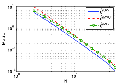
Figure 3: The performance of the ML, MVU, and U-V estimators for estimation after parameter selection with independent uniformly distributed populations and the SMS rule.

V-B Linear Gaussian model

Consider the following observation model:

$$\left\{\begin{array}[]{l}y_{1}[n]=\theta_{1}+w_{1}[n]\\ y_{2}[n]=\theta_{2}+w_{2}[n]\end{array}\right.,~{}~{}~{}n=0,\ldots,N-1,$$ (48)

where the normally distributed noise vectors, ${\bf{w}}[n]=[w_{1}[n],w_{2}[n]]^{\mbox{\tiny$T$}}$, $n=0,\ldots,N-1$, are independent in time and space and have a zero mean and a known covariance matrix,

$${\mbox{\boldmath$\Sigma$}}\stackrel{{\scriptstyle\triangle}}{{=}}\left[\begin{array}[]{cc}\sigma_{1}^{2}&0\\ 0&\sigma_{2}^{2}\end{array}\right].$$

We assume the SMS rule, which selects the population with the largest sample mean, i.e.,

$$\Psi_{{\text{SMS}}}=\arg\max_{m=1,2}\left\{\hat{\theta}_{m}^{({\mbox{\tiny ML}})}\right\},$$ (49)

where

$$\hat{\theta}_{m}^{({\mbox{\tiny ML}})}\stackrel{{\scriptstyle\triangle}}{{=}}\frac{1}{N}\sum_{n=0}^{N-1}y_{m}[n],$$ (50)

is the ML estimator of $\theta_{m}$ for $m=1,2$. According to (50), the ML estimators are jointly Gaussian random variables with means $\theta_{1}$, $\theta_{2}$ and covariance matrix $\frac{1}{N}{\mbox{\boldmath$\Sigma$}}$. Thus, for the SMS rule in (49), the probability of selecting population $m$ is:

$$\Pr(\Psi_{{\text{SMS}}}=m;{\mbox{\boldmath$\theta$}})=\Pr(\hat{\theta}_{m}^{({\mbox{\tiny ML}})}-\hat{\theta}_{k}^{({\mbox{\tiny ML}})}>0;{\mbox{\boldmath$\theta$}})=\Phi(\Delta_{m}),$$ (51)

for $m,k=1,2$, $m\neq k$, where $\Phi(\cdot)$ denotes the standard normal cumulative distribution function (cdf),

$$\Delta_{m}=\frac{\theta_{m}-\theta_{k}}{\sigma},~{}~{}~{}m,k=1,2,~{}m\neq k,$$

and $\sigma^{2}\stackrel{{\scriptstyle\triangle}}{{=}}\frac{\sigma_{1}^{2}+\sigma_{2}^{2}}{N}$.

V-B1 The $\Psi_{{\text{SMS}}}$-CRB

It can be verified that for this case

$$\nabla_{\mbox{\boldmath{\scriptsize$\theta$}}}^{2}\log f({\bf{x}};{\mbox{\boldmath$\theta$}})=-N{\mbox{\boldmath$\Sigma$}}^{-1}.$$ (52)

Therefore, by substituting (52) in (18), one obtains

$${\bf{J}}_{m}({\mbox{\boldmath$\theta$}},\Psi)=N{\mbox{\boldmath$\Sigma$}}^{-1}+\nabla_{\mbox{\boldmath{\scriptsize$\theta$}}}^{2}\log\Pr(\Psi=m;{\mbox{\boldmath$\theta$}}),~{}m=1,2,$$ (53)

for the selection rule $\Psi$. By substituting (53) in (9), the proposed $\Psi$-CRB is obtained. Therefore, by using (51), the chain, and the product rules, it can be verified that

$$\nabla_{\mbox{\boldmath{\scriptsize$\theta$}}}^{2}\log\Pr(\Psi_{{\text{SMS}}}=m;{\mbox{\boldmath$\theta$}})=\frac{c(\Delta_{m})}{\sigma^{2}}\left[\begin{array}[]{rr}1&-1\\ -1&1\end{array}\right],$$ (56)

for all $m=1,2$, where

$$c(\Delta)\stackrel{{\scriptstyle\triangle}}{{=}}-\frac{\phi(\Delta)}{\Phi(\Delta)}\Delta-\frac{\phi^{2}(\Delta)}{\Phi^{2}(\Delta)}$$ (57)

and $\phi(\cdot)$ denotes the standard normal pdf. By substituting (56) in (53), one obtains

$${\bf{J}}_{m}^{-1}({\mbox{\boldmath$\theta$}},\Psi)=\frac{1}{N}\left({\mbox{\boldmath$\Sigma$}}-\frac{c(\Delta_{m})}{N\sigma^{2}(c(\Delta_{m})+1)}{\bf{D}}\right),$$ (58)

where

$${\bf{D}}\stackrel{{\scriptstyle\triangle}}{{=}}\left[\begin{array}[]{cc}\sigma_{1}^{4}&-\sigma_{1}^{2}\sigma_{2}^{2}\\ -\sigma_{1}^{2}\sigma_{2}^{2}&\sigma_{2}^{4}\end{array}\right].$$ (61)

By substituting (58) in (11), we obtain the $\Psi_{\text{SMS}}$-CRB on the component-wise PSMSE:

$${\rm{E}}_{{\mbox{\boldmath{\scriptsize$\theta$}}}}\left[(\hat{\theta}_{m}-\theta_{m})^{2}|\Psi_{\text{SMS}}=m\right]\geq\frac{\sigma_{m}^{2}}{N}\zeta\left(\Delta_{m},\frac{\sigma_{m}^{2}}{\sigma_{1}^{2}+\sigma_{2}^{2}}\right),$$ (62)

$m,k=1,2$ and $m\neq k$, where

$$\zeta\left(\Delta,\kappa\right)\stackrel{{\scriptstyle\triangle}}{{=}}1-\frac{c(\Delta)}{c(\Delta)+1}\kappa.$$ (63)

Finally, by substituting (51) and (62) in (10), the $\Psi_{\text{SMS}}$-CRB on the PSMSE is obtained:

$$B^{(\Psi_{{\text{SMS}}})}({\mbox{\boldmath$\theta$}}) = \frac{\sigma_{1}^{2}}{N}\Phi\left(\Delta_{1}\right)\zeta\left(\Delta_{1},\frac{\sigma_{1}^{2}}{\sigma_{1}^{2}+\sigma_{2}^{2}}\right)$$ (64)

$$+\frac{\sigma_{2}^{2}}{N}\Phi\left(\Delta_{2}\right)\zeta\left(\Delta_{2},\frac{\sigma_{1}^{2}}{\sigma_{1}^{2}+\sigma_{2}^{2}}\right).$$

Similarly, the biased $\Psi$-CRB is obtained by substituting (58) and the gradient of the ML $\Psi$-biased from (65)-(66) in (III-C3).

It is well known that the conventional CRB, on estimating the $m$th parameter $\theta_{m}$ without a selection stage, is given by (e.g. [11] pp. 31-32) $\frac{\sigma_{m}^{2}}{N}$. Therefore, the component-wise $\Psi_{\text{SMS}}$-CRB in (62) is equal to the conventional marginal CRB multiplied by a correction factor, $\zeta\left(\Delta,\sigma_{1},\sigma_{2}\right)$, as defined in (63). The correction factor is presented in Fig. 4 versus $\Delta$ and $\sigma_{1}^{2}$ for $N=10$ and $\sigma_{2}=1$. It can be seen that for $\Delta<0$, the correction factor increases as $\Delta$ decreases, because this situation occurs when the order-relation of the sample means is wrong, which is an indication of high estimation error. Similarly, the correction factor increases as the variance $\sigma_{1}^{2}$ increases. In contrast, for $c(\Delta)=0$, which occurs when $\Delta\gg 0$, the correction factor satisfies $\zeta(\Delta,\sigma_{1},\sigma_{2})\rightarrow 1$ and thus, the component-wise $\Psi_{{\text{SMS}}}$-CRB converges to the CRB, i.e., the selection stage has only minor influence on the estimation stage. It should be noted, however, that the CRB and $\Psi_{{\text{SMS}}}$-CRB are lower bounds on different performance measures, i.e., MSE and PSMSE, and on different groups of estimators, i.e., mean-unbiased and $\Psi_{{\text{SMS}}}$-unbiased estimators, respectively.

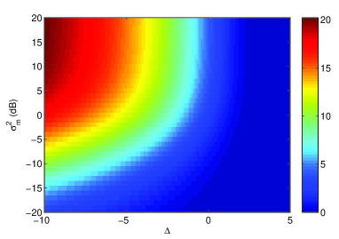
Figure 4: The multiplication factor, $\zeta(\Delta,\sigma_{1},\sigma_{2})$, for the linear Gaussian model with $N=10$ and $\sigma_{2}=1$.

V-B2 Estimation

In [9] it is shown that there is no $\Psi_{{\text{SMS}}}$-unbiased estimator of $\theta_{1}$ and $\theta_{2}$. It is also shown that the ML estimator satisfies [9]

$${\rm{E}}_{\mbox{\boldmath{\scriptsize$\theta$}}}\left[\left.\hat{\theta}_{m}^{({\mbox{\tiny ML}})}-\theta_{m}\right|\Psi_{{\text{SMS}}}=m\right]=\frac{\sigma_{m}^{2}}{N\sigma}\frac{\phi(\Delta_{m})}{\Phi(\Delta_{m})}\geq 0$$ (65)

and

$${\rm{E}}_{\mbox{\boldmath{\scriptsize$\theta$}}}\left[\left.\hat{\theta}_{k}^{({\mbox{\tiny ML}})}-\theta_{k}\right|\Psi_{{\text{SMS}}}=m\right]=-\frac{\sigma_{k}^{2}}{N\sigma}\frac{\phi(\Delta_{m})}{\Phi(\Delta_{m})}\leq 0,$$ (66)

$m,k=1,2$, $m\neq k$. This result indicates that the ML tends to overestimate the parameter of the selected population and to underestimate the unknown parameter of the unselected population.

By using the model in (48) and the selection probability in (51), we obtain the following post-selection likelihood function for the SMS rule:

$$\nabla_{\mbox{\boldmath{\scriptsize$\theta$}}}\log f({\bf{x}}|\Psi_{{\text{SMS}}}=m;{\mbox{\boldmath$\theta$}})=N{\mbox{\boldmath$\Sigma$}}^{-1}\left(\hat{{\mbox{\boldmath$\theta$}}}^{({\mbox{\tiny ML}})}-{\mbox{\boldmath$\theta$}}\right)$$

$$-\frac{\phi(\Delta_{m})}{\sigma\Phi(\Delta_{m})}\left[\begin{array}[]{c}{\mathbf{1}}_{\{{\bf{x}}\in{\mathcal{A}}_{1}\}}-{\mathbf{1}}_{\{{\bf{x}}\in{\mathcal{A}}_{2}\}}\\ {\mathbf{1}}_{\{{\bf{x}}\in{\mathcal{A}}_{2}\}}-{\mathbf{1}}_{\{{\bf{x}}\in{\mathcal{A}}_{1}\}}\end{array}\right],$$ (69)

where $\hat{{\mbox{\boldmath$\theta$}}}^{({\mbox{\tiny ML}})}=[\hat{\theta}_{1}^{({\mbox{\tiny ML}})},\hat{\theta}_{2}^{({\mbox{\tiny ML}})}]^{\mbox{\tiny$T$}}$ is defined in (50). According to (31), by equating the r.h.s. of (V-B2) to zero we obtain the PSML estimator for ${\bf{x}}\in{\mathcal{A}}_{m}$:

$$\hat{{\mbox{\boldmath$\theta$}}}^{({\mbox{\tiny PSML}})}=\hat{{\mbox{\boldmath$\theta$}}}^{({\mbox{\tiny ML}})}\hskip 142.26378pt$$

$$-\frac{1}{N\sigma}\frac{\phi(\hat{\Delta}_{m}^{({\mbox{\tiny PSML}})})}{\Phi(\hat{\Delta}_{m}^{({\mbox{\tiny PSML}})})}\left[\begin{array}[]{c}\sigma_{1}^{2}\left({\mathbf{1}}_{\{{\bf{x}}\in{\mathcal{A}}_{1}\}}-{\mathbf{1}}_{\{{\bf{x}}\in{\mathcal{A}}_{2}\}}\right)\\ \sigma_{2}^{2}\left({\mathbf{1}}_{\{{\bf{x}}\in{\mathcal{A}}_{2}\}}-{\mathbf{1}}_{\{{\bf{x}}\in{\mathcal{A}}_{1}\}}\right)\end{array}\right],$$ (72)

where

$$\hat{\Delta}_{m}^{({\mbox{\tiny PSML}})}=\frac{\hat{\theta}_{m}^{({\mbox{\tiny PSML}})}-\hat{\theta}_{k}^{({\mbox{\tiny PSML}})}}{\sigma},~{}~{}~{}m,k=1,2,~{}m\neq k,$$

for any ${\bf{x}}\in{\mathcal{A}}_{m}$. It can be seen that as $\sigma^{2}$ increases the correction term on the r.h.s. of (V-B2) becomes insignificant and the PSML estimator approaches the ML estimator.

The solution of (V-B2) can be found by an exhaustive search over $\hat{{\mbox{\boldmath$\theta$}}}^{({\mbox{\tiny PSML}})}$ or by using the iterative methods from Section IV-B. It can be verified that the Newton-Raphson and post-selection Fisher scoring coincide in this case, where the $i$th iteration of the Newton-Raphson PSML (NR-PSML) is obtained by substituting (V-B2) and (58) in (IV-B2). Similarly, by substituting (51), (52), and (56) in (38), the MBP estimator is obtained:

$$\hat{{\mbox{\boldmath$\theta$}}}^{(i+1)}=\hat{{\mbox{\boldmath$\theta$}}}^{({\mbox{\tiny ML}})}\hskip 170.71652pt$$

$$-\frac{\phi(\hat{\Delta}^{(i)})}{N\sigma\Phi(\hat{\Delta}^{(i)})}\left[\begin{array}[]{c}\sigma_{1}^{2}\left({\mathbf{1}}_{\{{\bf{x}}\in{\mathcal{A}}_{1}\}}-{\mathbf{1}}_{\{{\bf{x}}\in{\mathcal{A}}_{2}\}}\right)\\ \sigma_{2}^{2}\left({\mathbf{1}}_{\{{\bf{x}}\in{\mathcal{A}}_{2}\}}-{\mathbf{1}}_{\{{\bf{x}}\in{\mathcal{A}}_{1}\}}\right)\end{array}\right],$$ (75)

which coincides with the results in [48] for the Gaussian case.

The bias and PSMSE of the ML, NR-PSML, and MBP estimators with the SMS rule are evaluated using $20,000$ Monte-Carlo simulations, and the results are presented in Figs. 5 and 6, respectively, for $\theta_{1}=0$, $\theta_{2}=0.1$, $\sigma_{1}^{2}=1$, and $\sigma_{2}^{2}=0.1$. The PSMSE performance is compared to the $\Psi$-CRB from (64) and the biased $\Psi$-CRB. It can be seen that the PSML methods have a lower $\Psi$-bias and lower PSMSE than the ML estimator and that the MBP estimator has the best performance in both terms. Since no $\Psi$-unbiased estimator exists, the $\Psi_{{\text{SMS}}}$-CRB is higher than the actual PSMSE values, but the biased $\Psi$-CRB is a valid bound for any $N$. However, it can be seen that the $\Psi_{{\text{SMS}}}$-CRB gives an indication of the performance behavior and that asymptotically it is attained by the PSML estimator and coincides with the biased $\Psi$-CRB.

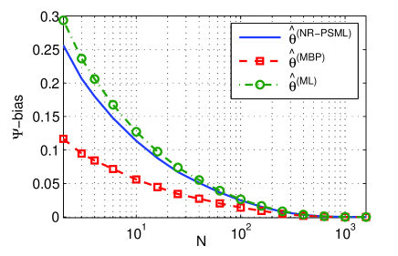
Figure 5: The $\Psi_{{\text{SMS}}}$-bias of the ML, NR-PSML, and MBP estimators for estimation after parameter selection with independent Gaussian distributed populations and the SMS rule.

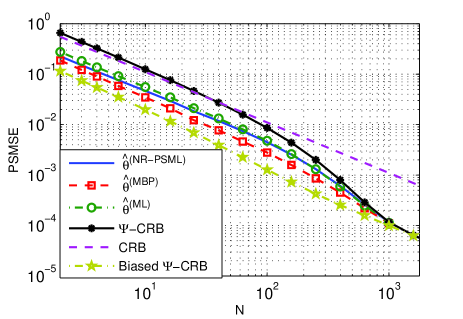
Figure 6: The PSMSE of the ML, NR-PSML, and MBP estimators and the $\Psi$-CRB for estimation after parameter selection with independent Gaussian distributed populations and the SMS rule.

V-C Exponential distribution

Consider the following observation model:

$$f_{m}(y_{m}[n];\theta_{m})=\left\{\begin{array}[]{lr}\frac{1}{\theta_{m}}e^{-\frac{y_{m}[n]}{\theta_{m}}}&0<y_{m}[n]\\ 0&{\text{otherwise}}\end{array}\right.,~{}m=1,2,$$ (78)

for all $n=0,\ldots,N-1$, where the parameters $\theta_{m}>0$ for all $m=1,2$ are unknown. The populations are assumed to be independent. In this problem, the SMS rule selects the population with the largest sample-mean, i.e.,

$$\Psi_{{\text{SMS}}}=\arg\max_{m=1,2}\left\{\hat{\theta}_{m}^{({\mbox{\tiny ML}})}\right\},$$ (79)

where

$$\hat{\theta}_{m}^{({\mbox{\tiny ML}})}\stackrel{{\scriptstyle\triangle}}{{=}}\frac{1}{N}\sum_{n=0}^{N-1}y_{m}[n]$$ (80)

is the ML estimator of $\theta_{m}$ for $m=1,2$. The probability of selecting population $m$ via the SMS rule is given by the negative binomial cdf [16]:

$$\Pr(\Psi_{{\text{SMS}}}=m;{\mbox{\boldmath$\theta$}})=\sum_{j=0}^{N-1}\left(\begin{array}[]{c}N+j-1\\ j\end{array}\right)q_{m}^{N}(1-q_{m})^{j}$$ (83)

for any $\theta_{m},\theta_{k}>0$, where $q_{m}\stackrel{{\scriptstyle\triangle}}{{=}}\frac{\theta_{m}}{\theta_{m}+\theta_{k}}$.

V-C1 Estimation

The ML estimator from (80) is an $\Psi_{{\text{SMS}}}$-biased estimator in this case, since [16]

$${\rm{E}}_{\mbox{\boldmath{\scriptsize$\theta$}}}\left[\left.\hat{\theta}_{m}^{({\mbox{\tiny ML}})}-\theta_{m}\right|\Psi_{{\text{SMS}}}=m\right]=\theta_{m}\alpha_{m}$$ (84)

for any $\theta_{m},\theta_{k}>0$, where $m,k=1,2$, $m\neq k$ and

$$\alpha_{m}\stackrel{{\scriptstyle\triangle}}{{=}}\frac{1}{\Pr(\Psi_{{\text{SMS}}}=m;{\mbox{\boldmath$\theta$}})}\left(\begin{array}[]{c}2N-1\\ N\end{array}\right)q_{m}^{N}(1-q_{m})^{N}.$$

In addition, by using (84) it can be verified that

$${\rm{E}}_{\mbox{\boldmath{\scriptsize$\theta$}}}\left[\left.\hat{\theta}_{k}^{({\mbox{\tiny ML}})}-\theta_{k}\right|\Psi_{{\text{SMS}}}=m\right]=-\theta_{k}\alpha_{m}$$ (85)

for any $\theta_{m},\theta_{k}>0$, where $m,k=1,2$, $m\neq k$. The $\Psi_{\text{SMS}}$-biases in (84) and (85) are positive and negative, respectively, thus they tend to overestimate the parameter of the selected population and underestimate that of the unselected one. As an alternative to the ML estimator, the following U-V estimator is proposed in [16]:

$$\hat{\theta}_{m}^{({\mbox{\tiny U-V}})}=\hat{\theta}_{m}^{({\mbox{\tiny ML}})}-\frac{\left(\hat{\theta}_{k}^{({\mbox{\tiny ML}})}\right)^{N}}{\left(\hat{\theta}_{m}^{({\mbox{\tiny ML}})}\right)^{N-1}},~{}m,k=1,2,~{}~{}m\neq k.$$ (86)

It is also shown that ${\rm{E}}_{\mbox{\boldmath{\scriptsize$\theta$}}}\left[\left(\hat{\theta}_{m}^{({\mbox{\tiny U-V}})}-{\theta}_{m}\right){\mathbf{1}}_{\{\Psi_{{\text{SMS}}}=m\}}\right]=0$ and thus, according to (5), the U-V estimator is an $\Psi_{{\text{SMS}}}$-unbiased estimator.

In the following, we derive the PSML estimator for $\Psi_{{\text{SMS}}}=m$. The results for $\Psi_{{\text{SMS}}}=k$, $k\neq m$ are straightforward. For the sake of simplicity, the elements of $\theta$ are reordered such that the first element is the selected one, i.e., ${\mbox{\boldmath$\theta$}}=[\theta_{m},\theta_{k}]^{\mbox{\tiny$T$}}$. The PSML estimator from (30) maximizes the post-selection likelihood, which is given in this case by

$$\log f({\bf{x}}|\Psi_{{\text{SMS}}}=m;{\mbox{\boldmath$\theta$}})$$ (89)

$$= -N\log\theta_{m}-N\log\theta_{k}-\frac{N\hat{\theta}_{m}^{({\mbox{\tiny ML}})}}{\theta_{m}}-\frac{N\hat{\theta}_{k}^{({\mbox{\tiny ML}})}}{\theta_{k}}$$

$$-\log\left(\sum_{j=0}^{N-1}\left(\begin{array}[]{c}N+j-1\\ j\end{array}\right)q_{m}^{N}(1-q_{m})^{j}\right)$$

for any $\theta_{m},\theta_{k}>0$ and ${\bf{x}}\in{\mathcal{A}}_{m}$. By using (89), it can be verified that the gradient vector of $f({\bf{x}}|\Psi_{{\text{SMS}}}=m;{\mbox{\boldmath$\theta$}})$ w.r.t. $\theta$ is given by

$$\nabla_{\mbox{\boldmath{\scriptsize$\theta$}}}\log f({\bf{x}}|\Psi_{{\text{SMS}}}=m;{\mbox{\boldmath$\theta$}})=N\left[\begin{array}[]{c}\frac{\hat{\theta}_{m}^{({\mbox{\tiny ML}})}-\theta_{m}+\theta_{m}f(q_{m})}{\theta_{m}^{2}}\\ \frac{\hat{\theta}_{k}^{({\mbox{\tiny ML}})}-\theta_{k}-\theta_{k}f(q_{m})}{\theta_{k}^{2}}\end{array}\right],$$ (92)

for any $\theta_{m},\theta_{k}>0$, $m,k=1,2$, and $m\neq k$, where

$$f(q_{m})\stackrel{{\scriptstyle\triangle}}{{=}}(1-q_{m})(q_{m}h(q_{m})-1)$$ (93)

and

$$h(q_{m})\stackrel{{\scriptstyle\triangle}}{{=}}\frac{\sum_{j=0}^{N-2}\left(\begin{array}[]{c}N+j\\ j\end{array}\right)q_{m}^{N}(1-q_{m})^{j}}{\Pr(\Psi_{\text{SMS}}=m;{\mbox{\boldmath$\theta$}})},~{}m=1,2.$$ (94)

According to (31), by equating the r.h.s. of (92) to zero we obtain the PSML estimator for ${\bf{x}}\in{\mathcal{A}}_{m}$:

$$\left[\begin{array}[]{c}\hat{\theta}_{m}^{({\mbox{\tiny PSML}})}\\ \hat{\theta}_{k}^{({\mbox{\tiny PSML}})}\end{array}\right]=\left[\begin{array}[]{c}\frac{\hat{\theta}_{m}^{({\mbox{\tiny ML}})}}{1-f(\hat{q}_{m})}\\ \frac{\hat{\theta}_{k}^{({\mbox{\tiny ML}})}}{1+f(\hat{q}_{m})}\end{array}\right],$$ (99)

where $\hat{q}_{m}\stackrel{{\scriptstyle\triangle}}{{=}}\frac{\hat{\theta}_{m}^{({\mbox{\tiny PSML}})}}{\hat{\theta}_{m}^{({\mbox{\tiny PSML}})}+\hat{\theta}_{k}^{({\mbox{\tiny PSML}})}}$ and ${\bf{x}}\in{\mathcal{A}}_{m}$. Equation (99) implies that the ratios $\frac{\hat{\theta}_{m}^{({\mbox{\tiny PSML}})}}{\hat{\theta}_{m}^{({\mbox{\tiny ML}})}}$ and $\frac{\hat{\theta}_{k}^{({\mbox{\tiny PSML}})}}{\hat{\theta}_{k}^{({\mbox{\tiny ML}})}}$ are only functions of the statistic $\frac{\hat{\theta}_{k}^{({\mbox{\tiny ML}})}}{\hat{\theta}_{m}^{({\mbox{\tiny ML}})}}$. That is, the PSML estimator is a function of the ML estimator multiplied by a correction factor, which is a function of the ML estimators’ ratio.

The solution to (99) can be found for the general case by an exhaustive search over $\hat{{\mbox{\boldmath$\theta$}}}^{({\mbox{\tiny PSML}})}$ or by using the iterative methods from Section IV-B. For example, by substituting (83), (52), and (56) in (38), the $i$th iteration of the MBP method is obtained.

V-C2 $\Psi_{\text{SMS}}$-CRB

The PSFIM can be obtained by using the derivative of (92), applying the expectation operator, and using (84) and (85). Then, the $\Psi_{\text{SMS}}$-CRB is obtained by substituting the PSFIM in (10). The explicit $\Psi_{\text{SMS}}$-CRB is omitted from this paper due to space limitation.

V-C3 $\Psi_{\text{SMS}}$-efficiency

For the special case of $N=1$, it can be shown that the $\Psi_{\text{SMS}}$-CRB is given by

$$B^{(\Psi_{{\text{SMS}}})}({\mbox{\boldmath$\theta$}})=\frac{\theta_{m}^{3}+\theta_{k}^{3}}{\theta_{m}+\theta_{k}}.$$ (100)

The PSML estimator in this case is given by

$$\left[\begin{array}[]{c}\hat{\theta}_{m}^{({\mbox{\tiny PSML}})}\\ \hat{\theta}_{m}^{({\mbox{\tiny PSML}})}\end{array}\right]=\left[\begin{array}[]{c}y_{m}[0]-y_{k}[0]\\ y_{k}[0]\frac{y_{m}[0]-y_{k}[0]}{y_{m}[0]-2y_{k}[0]}\end{array}\right]$$ (105)

for any $y_{m}[0]\geq y_{k}[0]$ and $y_{m}[0]\neq 2y_{k}[0]$. For $y_{k}[0]\geq y_{m}[0]$, we can change the roles of $\theta_{m}$ and $\theta_{k}$ to obtain the PSML estimator. It can be seen that for $N=1$, the PSML and U-V estimators from (105) and (86), respectively, of the selected parameter coincides, i.e., $\hat{\theta}_{m}^{({\mbox{\tiny PSML}})}=\hat{\theta}_{m}^{({\mbox{\tiny U-V}})}$. Thus, the PSML estimator is an $\Psi_{\text{SMS}}$-unbiased estimator for $N=1$. In addition, we can verify analytically that the PSMSE of $\hat{{\mbox{\boldmath$\theta$}}}^{({\mbox{\tiny PSML}})}$ attains the $\Psi_{\text{SMS}}$-CRB from (100). Thus, $\hat{{\mbox{\boldmath$\theta$}}}^{({\mbox{\tiny PSML}})}$ is an $\Psi_{\text{SMS}}$-efficient estimator for $N=1$.

The PSMSE performance of the estimators $\hat{{\mbox{\boldmath$\theta$}}}^{({\mbox{\tiny ML}})}$ and $\hat{{\mbox{\boldmath$\theta$}}}^{({\mbox{\tiny PSML}})}$ with the SMS rule are evaluated using $100,000$ Monte-Carlo simulations and are compared with the $\Psi_{\text{SMS}}$-CRB for $N=1$ and $\theta_{1}=5$. The results are presented in Figs. 7 and 8. It can be seen that the PSML estimator is an $\Psi$-unbiased estimator and has a lower PSMSE than the ML estimator. Moreover, the $\Psi_{{\text{SMS}}}$-CRB is achievable by $\hat{{\mbox{\boldmath$\theta$}}}^{({\mbox{\tiny PSML}})}$, which is an $\Psi_{\text{SMS}}$-efficient estimator in this case.

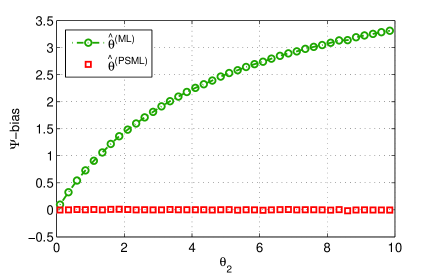
Figure 7: The $\Psi_{{\text{SMS}}}$-bias of the ML and PSML estimators for estimation after parameter selection with independent exponential distributed populations and the SMS rule.

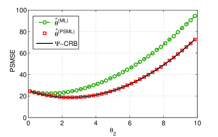
Figure 8: The PSMSE of the ML and PSML estimators and the $\Psi$-CRB for estimation after parameter selection with independent exponential distributed populations and the SMS rule.

VI Conclusion

In this paper, the concept of non-Bayesian estimation after parameter selection is introduced and the $\Psi$-unbiasedness in the Lehmann sense is defined, for arbitrary data-driven parameter selection rules. We derive a Cram$\acute{\text{e}}$r-Rao-type bound for the selected deterministic parameters. Unlike the conventional CRB, the proposed $\Psi$-CRB provides a valid bound in estimation after parameter selection problems. The PSML estimator is proposed and its properties and practical implementations aspects are discussed. In particular, it is proved that if there exists an $\Psi$-efficient estimator, then it is produced by the PSML estimator. The new paradigm opens a wide range of interesting directions, such as multistage procedures that involve active learning and sequential data sampling.

Appendix A: Proof of Proposition 1

In this Appendix, we prove Proposition 1 in a similar way to the proof of mean-unbiasedness under a conventional squared error cost function (Page 11 in [13]). By substituting the PSSE cost function from (2) in (4) the Lehmann-unbiasedness condition is given by

$${\rm{E}}_{{\mbox{\boldmath{\scriptsize$\theta$}}}}\left[\sum_{m=1}^{M}(\hat{\theta}_{m}-\eta_{m})^{2}{\mathbf{1}}_{\{\Psi=m\}}\right]\geq\hskip 78.24507pt$$

$${\rm{E}}_{{\mbox{\boldmath{\scriptsize$\theta$}}}}\left[\sum_{m=1}^{M}(\hat{\theta}_{m}-\theta_{m})^{2}{\mathbf{1}}_{\{\Psi=m\}}\right],~{}~{}~{}\forall{\mbox{\boldmath$\theta$}},{\mbox{\boldmath$\eta$}}\in{\mathbb{R}}^{M},$$ (106)

where ${\mbox{\boldmath$\eta$}}=[\eta_{1},\ldots,\eta_{M}]^{\mbox{\tiny$T$}}$ is an arbitrary vector. The condition in (Appendix A: Proof of Proposition 1) can be rewritten as

$${\rm{E}}_{{\mbox{\boldmath{\scriptsize$\theta$}}}}\left[\sum_{m=1}^{M}(\hat{\theta}_{m}-\theta_{m}+\theta_{m}-\eta_{m})^{2}{\mathbf{1}}_{\{\Psi=m\}}\right]\hskip 42.67912pt$$

$$\geq{\rm{E}}_{{\mbox{\boldmath{\scriptsize$\theta$}}}}\left[\sum_{m=1}^{M}(\hat{\theta}_{m}-\theta_{m})^{2}{\mathbf{1}}_{\{\Psi=m\}}\right],~{}~{}~{}\forall{\mbox{\boldmath$\theta$}},{\mbox{\boldmath$\eta$}}\in{\mathbb{R}}^{M}.$$ (107)

By using the linearity of the expectation operator and the fact that $\theta$ and $\eta$ are deterministic vectors, it can be verified that (Appendix A: Proof of Proposition 1) is equivalent to

$$\sum_{m=1}^{M}(\theta_{m}-\eta_{m}){\rm{E}}_{{\mbox{\boldmath{\scriptsize$\theta$}}}}\left[(\hat{\theta}_{m}-\theta_{m}){\mathbf{1}}_{\{\Psi=m\}}\right]$$

$$\geq-\sum_{m=1}^{M}(\theta_{m}-\eta_{m})^{2}\Pr(\Psi=m;{\mbox{\boldmath$\theta$}}),$$ (108)

$\forall{\mbox{\boldmath$\theta$}},{\mbox{\boldmath$\eta$}}\in{\mathbb{R}}^{M}$, where we used ${\rm{E}}_{{\mbox{\boldmath{\scriptsize$\theta$}}}}\left[{\mathbf{1}}_{\{\Psi=m\}}\right]=\Pr(\Psi=m;{\mbox{\boldmath$\theta$}})$. .
Sufficient condition - It can be verified that if (5) holds, then the inequality in (Appendix A: Proof of Proposition 1) holds since the r.h.s. of (Appendix A: Proof of Proposition 1) is nonpositive.
Necessary condition - The necessity of (5) is proven by using specific choices of $\eta$. By substituting $\eta_{m}=\theta_{m}$, for all $m=1,\ldots,M$, $m\neq l$, and $\eta_{l}=\theta_{l}+\varepsilon$ in (Appendix A: Proof of Proposition 1), we obtain the following necessary condition:

$$\varepsilon{\rm{E}}_{{\mbox{\boldmath{\scriptsize$\theta$}}}}\left[(\hat{\theta}_{l}-\theta_{l}){\mathbf{1}}_{\{\Psi=l\}}\right]\geq-\varepsilon^{2}\Pr(\Psi=l;{\mbox{\boldmath$\theta$}})$$ (109)

for any ${\mbox{\boldmath$\theta$}}\in{\mathbb{R}}^{M}$, $\varepsilon\in{\mathbb{R}}$. Since $\varepsilon$ can be either positive or negative and $\Pr(\Psi=l;{\mbox{\boldmath$\theta$}})\geq 0$, the condition in (109) implies (5) for any $l=1,\ldots,M$. In addition, since

$${\rm{E}}_{{\mbox{\boldmath{\scriptsize$\theta$}}}}[(\hat{\theta}_{m}-\theta_{m}){\mathbf{1}}_{\{\Psi=m\}}]={\rm{E}}_{{\mbox{\boldmath{\scriptsize$\theta$}}}}[\hat{\theta}_{m}-\theta_{m}|\Psi=m]\Pr(\Psi=m;{\mbox{\boldmath$\theta$}}),$$

$m=1,\ldots,M$, then, for any $m=1,\ldots,M$ such that $\Pr(\Psi=m;{\mbox{\boldmath$\theta$}})\neq 0$, the condition in (5) is equivalent to (6).

Appendix B. Proof of Lemma 1

In this Appendix, two alternative formulations of the PSFIM are derived. Similar derivations can be found in [26] in the context of post-detection estimation. By using (1), one obtains

$$\nabla_{\mbox{\boldmath{\scriptsize$\theta$}}}\log f({\bf{x}}|\Psi=m;{\mbox{\boldmath$\theta$}})\hskip 113.81102pt$$

$$=\nabla_{\mbox{\boldmath{\scriptsize$\theta$}}}\log f({\bf{x}};{\mbox{\boldmath$\theta$}})-\nabla_{\mbox{\boldmath{\scriptsize$\theta$}}}\Pr(\Psi=m;{\mbox{\boldmath$\theta$}}),$$ (110)

$\forall{\bf{x}}\in{\mathcal{A}}_{m}$, and by substituting (Appendix B. Proof of Lemma 1) in (7), one obtains

$${\bf{J}}_{m}({\mbox{\boldmath$\theta$}},\Psi)=\hskip 163.60333pt$$

$${\rm{E}}_{{\mbox{\boldmath{\scriptsize$\theta$}}}}\left[\left.\nabla_{\mbox{\boldmath{\scriptsize$\theta$}}}\log f({\bf{x}};{\mbox{\boldmath$\theta$}})\nabla_{\mbox{\boldmath{\scriptsize$\theta$}}}^{T}\log f({\bf{x}};{\mbox{\boldmath$\theta$}})\right|\Psi=m\right]\hskip 25.6073pt$$

$$-\nabla_{\mbox{\boldmath{\scriptsize$\theta$}}}\log\Pr(\Psi=m;{\mbox{\boldmath$\theta$}}){\rm{E}}_{{\mbox{\boldmath{\scriptsize$\theta$}}}}\left[\left.\nabla_{\mbox{\boldmath{\scriptsize$\theta$}}}^{T}\log f({\bf{x}};{\mbox{\boldmath$\theta$}})\right|\Psi=m\right]$$

$$-{\rm{E}}_{{\mbox{\boldmath{\scriptsize$\theta$}}}}\left[\left.\nabla_{\mbox{\boldmath{\scriptsize$\theta$}}}\log f({\bf{x}};{\mbox{\boldmath$\theta$}})\right|\Psi=m\right]\nabla_{\mbox{\boldmath{\scriptsize$\theta$}}}^{T}\log\Pr(\Psi=m;{\mbox{\boldmath$\theta$}})$$

$$+\nabla_{\mbox{\boldmath{\scriptsize$\theta$}}}\log\Pr(\Psi=m;{\mbox{\boldmath$\theta$}})\nabla_{\mbox{\boldmath{\scriptsize$\theta$}}}^{T}\log\Pr(\Psi=m;{\mbox{\boldmath$\theta$}}).\hskip 25.6073pt$$ (111)

Since ${\mathcal{A}}_{m}$ is independent of $\theta$ and by using regularity condition C.2, it can be noticed that

$$\nabla_{\mbox{\boldmath{\scriptsize$\theta$}}}\log\Pr(\Psi=m;{\mbox{\boldmath$\theta$}})=\frac{\nabla_{\mbox{\boldmath{\scriptsize$\theta$}}}\Pr(\Psi=m;{\mbox{\boldmath$\theta$}})}{\Pr(\Psi=m;{\mbox{\boldmath$\theta$}})}$$ (112)

$$= \frac{\nabla_{\mbox{\boldmath{\scriptsize$\theta$}}}\int_{{\mathcal{A}}_{m}}f({\bf{x}};{\mbox{\boldmath$\theta$}})\,\mathrm{d}{\bf{x}}}{\Pr(\Psi=m;{\mbox{\boldmath$\theta$}})}=\frac{\int_{{\mathcal{A}}_{m}}\nabla_{\mbox{\boldmath{\scriptsize$\theta$}}}f({\bf{x}};{\mbox{\boldmath$\theta$}})\,\mathrm{d}{\bf{x}}}{\Pr(\Psi=m;{\mbox{\boldmath$\theta$}})}$$

$$= {\rm{E}}_{{\mbox{\boldmath{\scriptsize$\theta$}}}}\left[\left.\nabla_{\mbox{\boldmath{\scriptsize$\theta$}}}\log f({\bf{x}};{\mbox{\boldmath$\theta$}})\right|\Psi=m\right].$$

Substitution of (112) in (Appendix B. Proof of Lemma 1) results in (1).

In addition, under the assumption that the integral $\int_{{\mathcal{A}}_{m}}f({\bf{x}}|\Psi=m;{\mbox{\boldmath$\theta$}}){\,\mathrm{d}}{\bf{x}}$ can be twice differentiated under the integral sign, it is known that (Lemma 2.5.3 in [36]):

$${\rm{E}}_{{\mbox{\boldmath{\scriptsize$\theta$}}}}\left[\left.\nabla_{\mbox{\boldmath{\scriptsize$\theta$}}}\log f({\bf{x}}|\Psi=m;{\mbox{\boldmath$\theta$}})\right|\Psi=m\right]=0$$

for any ${\mbox{\boldmath$\theta$}}\in{\mathbb{R}}^{M}$. Therefore, by using the product rule twice we obtain

$${\bf{J}}_{m}({\mbox{\boldmath$\theta$}},\Psi) = {\rm{E}}_{{\mbox{\boldmath{\scriptsize$\theta$}}}}\left[\left.\nabla_{\mbox{\boldmath{\scriptsize$\theta$}}}\log f({\bf{x}}|\Psi=m;{\mbox{\boldmath$\theta$}})\right.\right.$$ (113)

$$\times\left.\left.\nabla_{\mbox{\boldmath{\scriptsize$\theta$}}}^{T}\log f({\bf{x}}|\Psi=m;{\mbox{\boldmath$\theta$}})\right|\Psi=m\right]$$

$$= \nabla_{\mbox{\boldmath{\scriptsize$\theta$}}}{\rm{E}}_{{\mbox{\boldmath{\scriptsize$\theta$}}}}\left[\left.\nabla_{\mbox{\boldmath{\scriptsize$\theta$}}}^{T}\log f({\bf{x}}|\Psi=m;{\mbox{\boldmath$\theta$}})\right|\Psi=m\right]$$

$$-{\rm{E}}_{{\mbox{\boldmath{\scriptsize$\theta$}}}}\left[\left.\nabla_{\mbox{\boldmath{\scriptsize$\theta$}}}^{2}\log f({\bf{x}}|\Psi=m;{\mbox{\boldmath$\theta$}})\right|\Psi=m\right]$$

$$= -{\rm{E}}_{{\mbox{\boldmath{\scriptsize$\theta$}}}}\left[\left.\nabla_{\mbox{\boldmath{\scriptsize$\theta$}}}^{2}\log f({\bf{x}}|\Psi=m;{\mbox{\boldmath$\theta$}})\right|\Psi=m\right].$$

By substituting (Appendix B. Proof of Lemma 1) in (113), we obtain (18).

Appendix C: Numerical PSML estimation method

In some instances, the post-selection likelihood function and its gradient are intractable, so that finding the PSML, even by the iterative methods in (IV-B3) and (IV-B3), may be difficult. In these cases, we can use the previous estimator $\hat{{\mbox{\boldmath$\theta$}}}^{(i)}$ to construct a nonparametric estimator of ${\bf{g}}_{m}({\mbox{\boldmath$\theta$}})\stackrel{{\scriptstyle\triangle}}{{=}}\nabla_{\mbox{\boldmath{\scriptsize$\theta$}}}\log\Pr(\Psi=m;{\mbox{\boldmath$\theta$}})$ at ${\mbox{\boldmath$\theta$}}=\hat{{\mbox{\boldmath$\theta$}}}^{(i)}$ from simulated realizations of the observation model and then, to substitute them in (IV-B3) or (IV-B3). The resulting iterative PSML (IPSML) algorithm is described in Table I.

TABLE I: The IPSML algorithm

Initialization: Fix $i=0$ and set the temporary estimator $\hat{{\mbox{\boldmath$\theta$}}}^{(0)}=\hat{{\mbox{\boldmath$\theta$}}}^{({\mbox{\tiny ML}})}$.

Main iteration: Increment $i\rightarrow i+1$ and apply 1. Empirical gradient: For any $l=1,\ldots,M$: (a) Generate data $\tilde{{\bf{x}}}_{k}^{+}$ and $\tilde{{\bf{x}}}_{k}^{-}$ according to the pdf’s $f(\cdot;\hat{{\mbox{\boldmath$\theta$}}}^{(i)}+\frac{\Delta}{2}{\bf{e}}_{l})$ and $f(\cdot;\hat{{\mbox{\boldmath$\theta$}}}^{(i)}-\frac{\Delta}{2}{\bf{e}}_{l})$ for $k=1,\ldots,K$. (b) Evaluate the empirical partial derivative by: $\displaystyle\left[\hat{{\bf{g}}}_{m}\left({\mbox{\boldmath$\theta$}}=\hat{{\mbox{\boldmath$\theta$}}}^{(i)}\right)\right]_{l}\approx\frac{1}{\Delta}\times\hskip 85.35826pt$ $\displaystyle\log\left(\frac{1}{K}\sum\limits_{k=1}^{K}{\mathbf{1}}_{\Psi(\tilde{{\bf{x}}}_{k}^{+})=m}\right)-\log\left(\frac{1}{K}\sum\limits_{k=1}^{K}{\mathbf{1}}_{\Psi(\tilde{{\bf{x}}}_{k}^{-})=m}\right).$ (c) Update gradient: $\displaystyle\left.\nabla_{\mbox{\boldmath{\scriptsize$\theta$}}}\log f({\bf{x}}|\Psi=m;{\mbox{\boldmath$\theta$}})\right|_{{\mbox{\boldmath{\scriptsize$\theta$}}}=\hat{{\mbox{\boldmath{\scriptsize$\theta$}}}}^{(i)}}\hskip 42.67912pt$ $\displaystyle\approx\left.\nabla_{\mbox{\boldmath{\scriptsize$\theta$}}}f({\bf{x}};{\mbox{\boldmath$\theta$}})\right|_{{\mbox{\boldmath{\scriptsize$\theta$}}}=\hat{{\mbox{\boldmath{\scriptsize$\theta$}}}}^{(i)}}-\hat{{\bf{g}}}_{m}({\mbox{\boldmath$\theta$}}=\hat{{\mbox{\boldmath$\theta$}}}^{(i)}).$ (114) (d) Update estimation: Substitute (1c) in (IV-B3) or (IV-B3). 2. Stopping rule: iterate till convergence Output: $\hat{{\mbox{\boldmath$\theta$}}}^{({\mbox{\tiny IPSML}})}=\hat{{\mbox{\boldmath$\theta$}}}^{(i)}$.

References

• [1] S. Haykin, “Cognitive radio: brain-empowered wireless communications,” IEEE Journal on Selected Areas in Communications, vol. 23, no. 2, pp. 201–220, Feb. 2005.
• [2] H. Godrich, A. Petropulu, and H. Poor, “Sensor selection in distributed multiple-radar architectures for localization: A knapsack problem formulation,” IEEE Trans. Signal Processing, vol. 60, no. 1, pp. 247–260, Jan. 2012.
• [3] J. Bowden and E. Glimm, “Unbiased estimation of selected treatment means in two-stage trials,” Biometrical Journal, vol. 50, no. 4, pp. 515–527, 2008.
• [4] S. Z$\ddot{\text{o}}$llner and J. K. Pritchard, “Overcoming the winner’s curse: Estimating penetrance parameters from case-control data,” American Journal of Human Genetics, vol. 80, pp. 605–615, 2007.
• [5] T. Zhao and A. Nehorai, “Distributed sequential Bayesian estimation of a diffusive source in wireless sensor networks,” IEEE Trans. Signal Processing, vol. 55, no. 4, pp. 1511–1524, Apr. 2007.
• [6] N. Mukhopadhyay and T. K. Solanky, Multistage Selection and Ranking Procedures: Second Order Asymptotics, ser. Statistics: A Series of Textbooks and Monographs.   CRC Press, 1994, vol. 142.
• [7] K. Sarkadi, “Estimation after selection,” Studia Scientarium Mathematicarum Hungarica, pp. 341–350, 1967.
• [8] J. Putter and D. Rubinstein, “On estimating the mean of a selected population,” Technical Report, Department of Statistics, Univ. of Wisconsin, no. 165, 1968.
• [9] A. Cohen and H. B. Sackrowitz, “Estimating the mean of the selected population,” In: Gupta, S. S., Berger, J. O., eds. Statistical Decision Theory and Related Topics-III., vol. 1, pp. 247–270, 1982.
• [10] P. Vellaisamy, “A note on unbiased estimation following selection,” Statistical Methodology, vol. 6, no. 4, pp. 389–396, 2009.
• [11] S. M. Kay, Fundamentals of Statistical Signal Processing: Estimation Theory.   Upper Saddle River, NJ, USA: Prentice Hall, 1993.
• [12] A. D’Andrea, U. Mengali, and R. Reggiannini, “The modified Cram$\acute{\text{e}}$r-Rao bound and its application to synchronization problems,” IEEE Trans. Communications, vol. 42, no. 234, pp. 1391–1399, Feb. 1994.
• [13] E. L. Lehmann and J. P. Romano, Testing Statistical Hypotheses, 3rd ed.   New York: Springer Texts in Statistics, 2005.
• [14] J. D. Gibbons, I. Olkin, and M. Sobel, Selecting and Ordering Populations. A New Statistical Methodology.   New York: John Wiley and Sons., 1977.
• [15] X. Lu, A. Sun, and S. S. Wu, “On estimating the mean of the selected normal population in two-stage adaptive designs,” Journal of Statistical Planning and Inference, vol. 143, no. 7, pp. 1215–1220, 2013.
• [16] P. Vellaisamy and D. Sharma, “Estimation of the mean of the selected Gamma population,” Communications in Statistics - Theory and Methods, vol. 17, no. 8, pp. 2797–2817, 1988.
• [17] N. Misra, E. C. van der Meulen, and K. V. Branden, “On estimating the scale parameter of the selected Gamma population under the scale invariant squared error loss function,” Journal of Computational and Applied Mathematics, vol. 186, no. 1, pp. 268–282, 2006, special Issue: Jef Teugels.
• [18] R. Song, “On estimating the mean of the selected uniform population,” Communications in Statistics - Theory and Methods, vol. 21, no. 9, pp. 2707–2719, 1992.
• [19] J. Whitehead, “On the bias of maximum likelihood estimation following a sequential test,” Biometrika, vol. 73, no. 3, pp. 573–581, 1986.
• [20] N. Stallard and S. Todd, “Point estimates and confidence regions for sequential trials involving selection,” Journal of Statistical Planning and Inference, vol. 135, no. 2, pp. 402–419, 2005.
• [21] M. Carreras and W. Brannath, “Shrinkage estimation in two-stage adaptive designs with midtrial treatment selection,” Statistics in Medicine, vol. 32, no. 10, pp. 1677–1690, 2013.
• [22] H. Sackrowitz and E. Samuel-Cahn, “Evaluating the chosen population: A Bayes and minimax approach,” Lecture Notes-Monograph Series, vol. 8, pp. 386–399, 1986.
• [23] H. Robbins, “The UV method of estimation,” In: Gupta, S. S., Berger, J. O., eds. Statistical Decision Theory and Related Topics. IV, vol. 1, pp. 265–270, 1988.
• [24] E. Bashan, R. Raich, and A. Hero, “Optimal two-stage search for sparse targets using convex criteria,” IEEE Trans. Signal Processing, vol. 56, no. 11, pp. 5389–5402, Nov. 2008.
• [25] E. Bashan, G. Newstadt, and A. Hero, “Two-stage multiscale search for sparse targets,” IEEE Trans. Signal Processing, vol. 59, no. 5, pp. 2331–2341, May 2011.
• [26] E. Chaumette, P. Larzabal, and P. Forster, “On the influence of a detection step on lower bounds for deterministic parameter estimation,” IEEE Trans. Signal Processing, vol. 53, no. 11, pp. 4080–4090, Nov. 2005.
• [27] E. Chaumette and P. Larzabal, “Cram$\acute{\text{e}}$r-Rao bound conditioned by the energy detector,” IEEE Signal Processing Letters, vol. 14, no. 7, pp. 477–480, July 2007.
• [28] E. Fishler and H. Messer, “Order statistics approach for determining the number of sources using an array of sensors,” IEEE Signal Processing Letters, vol. 6, no. 7, pp. 179–182, July 1999.
• [29] ——, “Detection and parameter estimation of a transient signal using order statistics,” IEEE Trans. Signal Processing, vol. 48, no. 5, pp. 1455–1458, May 2000.
• [30] B. Efron, “Tweedie’s formula and selection bias,” Journal of the American Statistical Association, vol. 106, no. 496, pp. 1602–1614, 2011.
• [31] ——, “Estimation and accuracy after model selection,” Journal of the American Statistical Association, 2013.
• [32] J. Lee and J. Taylor, “Exact post model selection inference for marginal screening,” Preprint .arXiv paper 1402.5596v2., 2014.
• [33] S. Sando, A. Mitra, and P. Stoica, “On the Cram$\acute{\text{e}}$r-Rao bound for model-based spectral analysis,” IEEE Signal Processing Letters, vol. 9, no. 2, pp. 68–71, Feb. 2002.
• [34] Y. Noam and H. Messer, “Notes on the tightness of the hybrid Cram$\acute{\text{e}}$r-Rao lower bound,” IEEE Trans. Signal Processing, vol. 57, no. 6, pp. 2074–2084, June 2009.
• [35] T. Routtenberg and L. Tong, “The Cram$\acute{\text{e}}$r-Rao bound for estimation-after-selection,” in Proc. ICASSP 2014, May 2014, pp. 414–418.
• [36] E. L. Lehmann and G. Casella, Theory of Point Estimation (Springer Texts in Statistics), 2nd ed.   New York, NY: Springer, 1998.
• [37] T. Routtenberg and J. Tabrikian, “Non-Bayesian periodic Cram$\acute{\text{e}}$r-Rao bound,” IEEE Trans. Signal Processing, vol. 61, no. 4, pp. 1019–1032, Feb. 2013.
• [38] ——, “Cyclic Barankin-type bounds for non-Bayesian periodic parameter estimation,” IEEE Trans. Signal Processing, vol. 62, no. 13, pp. 3321–3336, July 2014.
• [39] J. V. Deshpande and T. M. Fareed, “A note on conditionally unbiased estimation after selection,” Statistics and Probability Letters, vol. 22, no. 1, pp. 17–23, 1995.
• [40] N. Nematollahi and F. Motamed-Shariati, “Estimation of the parameter of the selected uniform population under the entropy loss function,” Journal of Statistical Planning and Inference, vol. 142, no. 7, pp. 2190–2202, 2012.
• [41] E. W. Barankin, “Locally best unbiased estimates,” The Annals of Mathematical Statistics, vol. 20, no. 4, pp. 477–501, 1949.
• [42] E. Chaumette, J. Galy, A. Quinlan, and P. Larzabal, “A new Barankin bound approximation for the prediction of the threshold region performance of maximum likelihood estimators,” IEEE Trans. Signal Processing, vol. 56, no. 11, pp. 5319–5333, Nov. 2008.
• [43] K. Todros and J. Tabrikian, “General classes of performance lower bounds for parameter estimation Part I: Non-Bayesian bounds for unbiased estimators,” IEEE Trans. Information Theory, vol. 56, no. 10, pp. 5045–5063, Oct. 2010.
• [44] S. Jeyaratnam and S. Panchapakesan, “An estimation problem relating to subset selection for normal populations,” In: T.J. Santner and A.C. Tamhane, Marcel Dekker, eds. Design of Experiments; Ranking and Selection, vol. 1, pp. 287–302, 1984.
• [45] S. S. Gupta, “On some multiple decision (selection and ranking) rules,” Technometrics, vol. 7, no. 2, pp. pp. 225–245, 1965.
• [46] P. X.-K. Song, Y. Fan, and J. D. Kalbfleisch, “Maximization by parts in likelihood inference,” Journal of the American Statistical Association, vol. 100, no. 472, pp. 1145–1167, Dec. 2005.
• [47] J. G. Liao and B. F. Qaqish, “Discussion of maximization by parts in likelihood inference,” J. Amer. Statis. Assoc., vol. 100, pp. 1160–1161, 2005.
• [48] I. Bebu, G. Luta, and V. Dragalin, “Likelihood inference for a two-stage design with treatment selection,” Biometrical Journal, vol. 52, pp. 811–822, 2010.