A Virtual Element Method for elastic and inelastic problems on polytope meshes
Abstract
We present a Virtual Element Method (VEM) for possibly nonlinear elastic and inelastic problems, mainly focusing on a small deformation regime. The numerical scheme is based on a low-order approximation of the displacement field, as well as a suitable treatment of the displacement gradient. The proposed method allows for general polygonal and polyhedral meshes, it is efficient in terms of number of applications of the constitutive law, and it can make use of any standard black-box constitutive law algorithm. Some theoretical results have been developed for the elastic case. Several numerical results within the 2D setting are presented, and a brief discussion on the extension to large deformation problems is included.
1 Introduction
The Virtual Element Method (VEM), introduced in [2], is a recent generalization of the Finite Element Method which is characterized by the capability of dealing with very general polygonal/polyhedral meshes and the possibility to easily implement highly regular discrete spaces [11, 6]. Indeed, by avoiding the explicit construction of the local basis functions, the VEM can easily handle general polygons/polyhedrons without complex integrations on the element (see [4] for details on the coding aspects of the method). The interest in numerical methods that can make use of general polytopal meshes has recently undergone a significant growth in the mathematical and engineering literature. Among the large number of papers, we cite as a minimal sample [10, 5, 28, 19, 12, 30, 31, 17, 18, 16]. Indeed, polytopal meshes can be very useful for a wide range of reasons, including meshing of the domain (such as cracks) and data (such as inclusions) features, automatic use of hanging nodes, use of moving meshes, adaptivity.
In the framework of Structural Mechanics, recent applications of Polygonal Finite Element Methods, which is a different technology employing direct integration of complex non-polynomial functions, have shed light on some very interesting advantages of using general polygons to mesh the computational domain. This include, for instance, the greater robustness to mesh distortion [13], a reduced mesh sensitivity of solutions in topology optimization [12, 20], better handling of contact problems [7] and crack propagation [24]. Unfortunately, Polygonal Finite Elements suffer from some serious drawbacks, such as the strong difficulties in the three dimensional case (polyhedrons) and in the use of non convex elements. On the contrary, the VEM is free from the above-mentioned troubles, and thus it represents a very promising approach for Computational Structural Mechanics problems.
Aim of the present paper is to initiate the investigation on the VEM when applied to non-linear elastic and inelastic problems in small deformations. More precisely, we mainly focus on the following cases: 1) non-linear elastic constitutive laws in a small deformation regime which, however, pertain to stable materials; 2) inelastic constitutive laws in a small deformation regime as they arise, for instance, in classical plasticity problems. We remark that we are not going to consider here situations with internal constraints, such as incompressibility, which require additional peculiar numerical treatment. Virtual elements for the linear elasticity problem where introduced in [3, 21]. The scheme in the present paper is one of the very first developements of the VEM technology for nonlinear problems, and it is structured in such a way that a general non linear constitutive law can be automatically included. Indeed, on every element of the mesh the constitutive law needs only to be applied once (similarly to what happens in one-point Gauss quadrature scheme) and the constitutive law algorithm can be independently embedded as a self-standing black-box, as in common engineering FEM schemes. Therefore, in addition to the advantage of handling general polygons/polyhedra, the present method is computationally efficient, in the sense that the constitutive law needs to be applied only once per element at every iteration step. The risk of ensuing hourglass modes is avoided by using an evolution of the standard VEM stabilization procedure used in linear problems. However, we highlight that the proposed method is described for general -dimensional problems (), but the performed numerical experiments are confined to the two dimensional setting.
A brief outline of the paper is as follows. In Section 2 we describe the continuous problems we are interested in. In particular, we distinguish between the elastic, possibly non-linear, case (Section 2.1), and the general inelastic case (Section 2.2). Section 3 deals with the VEM discretization. After having introduced the approximation spaces and the necessary projection operators (Section 3.1), we detail the discrete problems for the elastic case in Section 3.2, and for the inelastic case in Section 3.3. In Section 4, combining ideas and techniques from [14] and [2], we provide some theoretical results concerning the convergence of the proposed scheme in the elastic situation. We remark that our analysis is confined to cases where the non-linear costitutive law fulfills suitable continuity and stability properties, as stated at the beginning of the Section. Section 5 presents several numerical examples which asses the actual behaviour of the proposed scheme. In Sections 5.1 and 5.2 we consider non-linear elastic cases, while in Section 5.3 a von Mises plasticity problem with hardening is detailed. Furthermore, an initial brief discussion about a possible extension to large deformation problem is included (Section 5.4). Finally, we draw some conclusion in Section 6.
Throughout the paper, we will make use of standard notations regarding Sobolev spaces, norms and seminorms, see [8], for instance. In addition, will denote a constant independent of the meshsize, not necessarily the same at each occurrence. Finally, given two real quantities and , we will write to mean that there exists such that .
2 The continuous problems
In the present section we describe the problem considered in this paper. Although the elastic case could be considered as a particular instance of the inelastic case, we prefer to keep the presentation of the two problems separate. This will allow us a clearer presentation of the ideas of the virtual element scheme in the following section.
2.1 The elastic case
We consider an elastic body () clamped on part of the boundary and subjected to a body load . We are interested, assuming a regime of small deformations, in finding the displacement of the deformed body.
We are given a constitutive law for the material at every point , relating strains to stresses , through the function
| (1) |
where represents the gradient of the displacement .
Let now denote the space of admissible displacements and the space of its variations; both spaces will, in particular, satisfy the homogeneous Dirichlet boundary condition on . The variational formulation of the elastic deformation problem reads
| (3) |
Remark 2.1.
The generalization of the results of the present paper to other type of loadings (for instance in the presence of boundary forces) and boundary conditions (for instance in the presence of enforced displacements) is trivial. Our choice in (2) allows to keep the exposition shorter.
2.2 The inelastic case
We assume a small deformation regime and restrict ourselves to rate independent inelasticity. We consider a material body () clamped on part of the boundary and subjected to a body load depending also on a pseudo-time variable . The interested reader can find more details in [23, 27], for instance. We are interested in finding the displacement of the deformed body at a given final time .
We are given an inelastic constitutive law for the material, relating strains to stresses , through the function
| (4) |
where the vector contains all history variables at the point .
The above rule is to be coupled with an evolution law for the history variables in time
| (5) |
where, as usual, a dot above a function stands for a pseudo-time derivative. Since we consider a quasi-static problem, at each time instant the stresses and displacements must satisfy the equilibrium and boundary conditions in (2).
We here avoid to write a rigorous variational formulation for the problem above, and limit ourselves to the minimal setting that will be needed to introduce the associated discrete problem. As in the elastic case, let denote the space of admissible displacements and the space of its variations. Then, assuming an initial value for the history variables, the quasi-static inelastic deformation problem can be written as
| (6) |
where the displacements and history variables are sufficiently regular in time and must satisfy the evolution law (5) almost everywhere.
3 The virtual element approximation
In the present section we introduce the virtual element discretization of problems (3) and (6). In what follows, given any subset of () and , we denote by (respectively ) the scalar (respectively vector with components) polynomials of degree up to on .
3.1 The virtual spaces and operators
We consider a mesh for the domain , made of general polygonal/polyhedral conforming elements. For the time being, we only assume that such mesh is compatible with the boundary conditions, i.e. that is union of faces (edges) of the mesh. We denote by the generic element of the mesh and by the generic face (or edge if ). The symbols and will represent, respectively, diameter and volume (or area) of the element . As usual, will indicate the maximum element size.
We start by introducing the discrete virtual space for displacements, that is essentially the same as in [3]. We first consider the two dimensional case. Given any , let the local virtual space
| (7) |
where denotes the component-wise Laplace operator. The space is a space of harmonic functions that on the boundary of the element are piecewise linear (edge by edge) and continuous. Such space is virtual in the sense that is well defined but not known explicitly inside the element.
Note that ; in the case of a triangular element, we recover exactly the standard space. It is easy to check [3] that a set of degrees of freedom for the space is simply given by the collection of the vertex values:
Once the above degrees of freedom values are given, since is linear on each edge, the value of on the boundary is completely determined. Therefore, an integration by parts allows to compute the integral average of the gradient
| (8) |
with indicating the outward unit normal at each edge .
We now define the virtual local spaces for the three dimensional case. Given a polyhedron , any face is now a polygon. We denote by the virtual bi-dimensional space (7) on the polygon adjusted with three components:
| (9) |
where the symbol represents the generic edge of the polyhedron and denotes the planar laplacian on . We then define
| (10) |
The space is a space of harmonic functions that on the boundary of the element are continuous and, on each face, functions of . Note that, as a consequence, the functions of are linear on each edge of the polyhedron.
Again we note that ; in the case of a tetrahedral element, we recover exactly the standard space. It is easy to check that a set of degrees of freedom for the space is again given by
An integration by parts exactly as in (8) allows to compute, for all the integral average of the gradient, provided one is able to compute the face integrals for all and . Such face integrals can be easily computed by introducing the virtual space modification proposed in [1], that we do not detail here. The result is
where the scalars are the weights of any integration rule on the face that is exact for linear functions.
Once the local virtual spaces are defined, all that follows holds identically in two and three dimensions. We can now present the global virtual space
A set of degrees of freedom for is given by all pointwise values of on all vertices of , excluding the vertices on (where the value vanishes).
In the following, we will denote by the tensor valued projection operator on the space of piecewise constant functions and by its restriction to the generic element . More precisely, for any , we have with the local operators defined as
| (11) |
We have the following important remark, which is a direct consequence of (8).
Remark 3.1.
For all functions and all elements , the operators are explicitly computable.
We moreover introduce a second projection operator , defined on as follows. For any , we have with the local operators defined as
| (12) |
for all in . Note that, by definition, is a (discontinuous) piecewise linear function on . On each element , is the unique linear function such that:
-
1.
its (constant) gradient equals the mean value over of the function ;
-
2.
its vertex value average equals the vertex value average of .
3.2 The elastic case
The main missing step is to introduce the local forms that will be used in the discrete variational formulation. We assume that the constitutive law (1) is piecewise constant with respect to the mesh . Therefore, instead of , we will write to represent the constitutive law on , and . In addition, foe every pair and , we introduce the bilinear forms and as:
| (15) |
We now consider, for all and all , the following preliminary form
| (16) | ||||
where the identity above follows since all the involved functions are constant on the element. The above form is -consistent, in the sense that it recovers exactly the original form whenever the first entry is a linear polynomial. Indeed, it follows from (11) and (12) that
| (17) | ||||
However, unless the elements are triangular/tetrahedral, the form has a non-physical kernel that may lead to spurious modes in the solution. We therefore follow the idea proposed initially in [2] and introduce the discrete bilinear form
| (18) | ||||
As discussed in [3, 2], under suitable mesh regularity assumptions detailed in Section 4, there exist positive constants independent of the element such that
| (19) |
for all with . In other words, on the orthogonal complement of with respect to , the bilinear form behaves as the local energy of a linearly elastic body with unitary material constants and is thus suitable to stabilize form in such case. In order to take into account different material constants and also nonlinear materials, the form needs to be multiplied by a positive constant that may depend on the discrete solution.
We therefore introduce the following local virtual form on . For all and all
| (20) |
where the stabilizing parameter depends on the additional entry . We remark that the bilinear form is still -consistent. This follows from (17) and the observation that for every . The choice that we here propose for the parameter is
| (21) |
with representing any norm on the fourth order tensor space, for instance the maximum of the absolute values of all the entries, see Remark 3.2.
We present also the global form
| (22) |
Given , a possible virtual discretization of Problem (3) is
| (23) |
Above, the load approximation term
is a vertex-based quadrature rule with weights chosen to provide the exact integral on when applied to linear functions. Furthermore, a reasonable choice for could be .
We instead propose a modification of (23), that is more practical from the implementation viewpoint. We assume the usual incremental loading procedure for the solution of the nonlinear discrete problem: given a positive integer , let the partial loadings for all . Then, given the initial displacement (for instance the zero function), one applies for the iterative procedure
| (24) |
The final solution is then . The nonlinear problems above can be solved with the Newton scheme. Note that, since the stability constants (see (20)) are computed by using , the tangent matrix in the Newton iterations turns out to be simpler. Since is typically taken large (at least 10, but often much more) the effect of such modification is not detrimental for the discrete approximation; the constants are only used as scaling parameters and do not enter the accuracy of the algorithm.
We close the section with some observations regarding the local forms used in the scheme. First, we recall that the proposed forms are -consistent, in the sense that for all , we have:
| (25) |
Identity (25) is a fundamental condition for approximation and, in particular, guarantees the satisfaction of the patch test. Moreover, such forms are explicitly computable for any polygonal/polyhedral element (even non-convex). Finally, the constitutive law needs to be computed only once per element and thus the method, from this point of view, is as cheap as finite elements with one point gauss integration rule. This observation has an even bigger impact in the inelastic case, where the constitutive laws are typically more expensive to compute.
Remark 3.2.
The motivation for choice (21) and (24) is to better mimic the stability properties of the material for the current displacement. For materials in which the stress-strain incremental relation does not depend too strongly on the value of the current displacement, the constants can be taken as independent of . For instance, a scaling directly proportional to the local material constants could be used. On the other hand, the choice proposed in (21) and (24) give good results for a wider range of materials. Examples and investigations in this direction can be found in Section 5.
3.3 The inelastic case
We start by introducing a sub-division of the “time” interval into smaller intervals for , where for simplicity we assume that . We will denote the partial loadings by for all .
We assume, as in standard engineering procedures, a constitutive algorithm that is an approximation of the constitutive and evolution laws (4), (5). In Finite Element analysis, this pointwise algorithm can be coded independently from the global FE construction and can be regarded as a “black-box” procedure that is applied at every Gauss point and at every iteration step. In the present Virtual Element method, we want to keep the same approach; in other words, our scheme will be compatible with any black-box constitutive algorithm that follows in the general setting below and that can be imported from other independent sources.
We assume that the constitutive law is piecewise constant with respect to the mesh . Let represent the constitutive algorithm for the element . For any , given a value for the displacement gradient at time , a value for the history variables at time and a tentative value for the displacement gradient at time , the algorithm computes the stresses (and updates the history variables) at time . We thus write the computed stress as
As part of the approximation procedure of our method, we assume that the history variables are piecewise constant with respect to the mesh, and therefore write to represent the value assumed on the element at time . Consistently, will represent the collection of all .
In our scheme, instead of applying the constitutive algorithm at Gauss points, we make use of the projections introduced in the previous sections and of the same stabilization as in the elastic case. The Virtual Element scheme reads, for :
| (26) |
where the form
with, for all ,
Here above, the bilinear form and the scalar are calculated as already shown in (18) and (21), respectively. Note that, as already mentioned in Section 3.2, the constitutive algorithm needs to be applied only once per element.
4 Theoretical results
We here develop an error analysis for the method described in Section 3.2, under some additional hypotheses on the function . More precisely, we assume that the following properties are satisfied.
Hypotheses (RPC)
-
•
The function belongs to for every ;
-
•
for every , the differential satisfies
-
1.
there exists such that
(27) -
2.
there exists such that
(28)
-
1.
We moreover explicit here the shape regularity conditions that are needed for the theoretical results of the present paper. We assume that there exists a positive constant such that all the elements of the mesh sequence are star shaped with respect to a ball of radius and that all the edges of have length .
Lemma 4.1.
Proof.
We first note that (27) and (28), together with (21), imply the existence of positive constants and such that
| (32) |
| (33) |
Therefore, for every we have
| (34) |
by which
| (35) |
For every , we have (see (20))
| (36) | ||||
We now notice that (see (16))
| (37) | ||||
First using (33) with and , then recalling (12) we get
| (38) | ||||
In addition, we have, using (32) and (19):
| (39) | ||||
Combining (36) with (38) and (39), we infer
| (40) |
Summing up over all the elements, we get (29):
| (41) |
Theorem 4.1.
Proof.
Remark 4.1.
Corollary 4.1.
Following the same notation of Theorem 4.1, let moreover . Then the linear convergence bound holds
5 Numerical tests
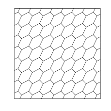
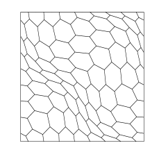
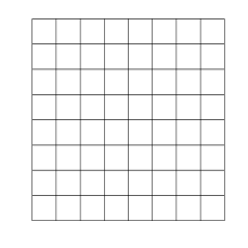
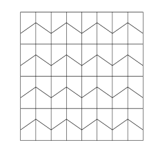
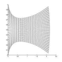
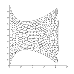
In the present section we test our virtual method. In the first two examples (see Sections 5.1 and 5.2), the body occupies the region , where lengths are expressed in meters. We employ the following types of mesh (see also Figures 1-2):
-
•
: Structured hexagonal meshes.
-
•
: Non-structured hexagonal meshes made of convex hexagons.
-
•
: Regular subdivisions of the domain in subsquares.
-
•
: Trapezoidal meshes which consist of partitions of the domain into congruent trapezoids, all similar to the trapezoid with vertexes , , , and .
In what follows, denotes the number of vertices in the mesh under consideration.
To test the convergence properties of the methods, we introduce the following discrete maximum norm: for any sufficiently regular function ,
| (54) |
where represents the set of vertexes of and denotes the vector norm. We also introduce the following discrete like norm:
| (55) |
where and denote the set of edges in the mesh and the length of the edge , respectively. Moreover, denotes one of the two tangent vectors to the edge , chosen once and for all. Accordingly, we denote by
the corresponding errors and we measure the experimental order of convergence as
where and denote the number of vertices in two consecutive meshes, with corresponding errors and .
5.1 Hencky-von Mises elasticity problem with analytical solution
The first constitutive law we consider, taken from [22], is the non-linear Hencky-von Mises elasticity model, for which
Here above, and are the nonlinear Lamé functions, is the small deformation strain tensor, the symbol represents the trace operator and is the Frobenius norm of the deviatoric part of the tensor .
We take the Lamé functions as follows:
This function corresponds to the Carreau law for viscoplastic materials. It is easy to verify that the hypotheses at the beginning of Section 4 are fulfilled by our choice of and . We have taken the load such that the solution of Problem (2) is given by:
In Table 1 we report the convergence history of the virtual method (24) applied to our test problem with different families of meshes. The table includes the number of mesh vertices, the convergence rates , and the discrete errors and .
| Mesh | |||||
|---|---|---|---|---|---|
| 64 | 3.4192e-2 | – | 4.5675e-1 | – | |
| 192 | 8.2511e-3 | 2.59 | 2.4445e-1 | 1.14 | |
| 640 | 2.4353e-3 | 2.03 | 1.2803e-1 | 1.07 | |
| 2304 | 6.7066e-4 | 2.01 | 6.5274e-2 | 1.05 | |
| 8704 | 1.7495e-4 | 2.02 | 3.2919e-2 | 1.03 | |
| 33792 | 4.4619e-5 | 2.01 | 1.6527e-2 | 1.02 | |
| 64 | 5.6458e-2 | – | 5.0007e-1 | – | |
| 192 | 1.9675e-2 | 1.92 | 2.7166e-1 | 1.11 | |
| 1280 | 6.4750e-3 | 1.85 | 1.4054e-1 | 1.09 | |
| 2304 | 2.01403-3 | 1.82 | 7.1120e-2 | 1.06 | |
| 8704 | 5.4860e-4 | 1.96 | 3.5590e-2 | 1.04 | |
| 33792 | 1.4070e-4 | 2.01 | 1.7817e-2 | 1.02 | |
| 25 | 6.1947e-2 | – | 7.1975e-1 | – | |
| 81 | 9.3599e-3 | 3.21 | 3.5627e-1 | 1.19 | |
| 578 | 1.7576e-3 | 2.62 | 1.7809e-1 | 1.09 | |
| 1089 | 4.2329e-4 | 2.14 | 8.9038e-2 | 1.04 | |
| 4225 | 1.0516e-4 | 2.05 | 4.4518e-2 | 1.02 | |
| 16641 | 2.6254e-5 | 2.02 | 2.2259e-2 | 1.01 | |
| 25 | 1.5401e-1 | – | 1.0516e-0 | – | |
| 81 | 3.3021e-2 | 2.62 | 5.3972e-1 | 1.14 | |
| 578 | 7.1005e-3 | 2.42 | 2.7525e-1 | 1.06 | |
| 1089 | 1.6650e-3 | 2.19 | 1.3832e-1 | 1.04 | |
| 4225 | 4.1133e-4 | 2.06 | 6.9382e-2 | 1.02 | |
| 16641 | 9.0462e-5 | 2.21 | 3.2452e-2 | 1.05 |
We observe from Table 1 that a clear first order convergence rate in the discrete like norm and show a quadratic rate in the discrete norm.
5.2 A benchmark elasticity model problem with analytical solution
In this test case, we select the constitutive load as
where is defined by the following nonlinear function:
with
We have taken the load such that the solution of Problem (2) is given by:
We remark that this choice does not actually correspond to any elastic material. Instead, it has been chosen as a “benchmark model” which does not satisfy the assumption at the begining of Section 4: condition (28) does not hold, in particular.
Table 2 shows the convergence history of the virtual method (24) applied to our test problem with different families of meshes. The table includes the number mesh vertices, the convergence rates , and the discrete errors and .
| Mesh | |||||
|---|---|---|---|---|---|
| 64 | 4.1122e-2 | – | 4.6371e-0 | – | |
| 192 | 1.7816e-2 | 1.52 | 2.6318e-0 | 1.03 | |
| 1280 | 5.0006e-3 | 2.11 | 1.3317e-0 | 1.13 | |
| 2304 | 1.2449e-3 | 2.17 | 6.6288e-1 | 1.08 | |
| 8704 | 2.9750e-4 | 2.15 | 3.3092e-1 | 1.04 | |
| 33792 | 8.2512e-5 | 1.90 | 1.6553e-1 | 1.02 | |
| 64 | 8.1685e-2 | – | 5.1698e-0 | – | |
| 192 | 2.3823e-2 | 2.24 | 2.9790e-0 | 1.00 | |
| 1280 | 1.4234e-2 | 0.86 | 1.5553e-0 | 1.08 | |
| 2304 | 5.9189e-3 | 1.37 | 7.6103e-1 | 1.12 | |
| 8704 | 1.7906e-3 | 1.80 | 3.6614e-1 | 1.10 | |
| 33792 | 4.7067e-4 | 1.97 | 1.7981e-1 | 1.05 | |
| 25 | 1.8457e-1 | – | 9.6706e-0 | – | |
| 81 | 5.2374e-2 | 2.14 | 4.0009e-0 | 1.50 | |
| 578 | 1.5787e-2 | 1.89 | 1.8538e-0 | 1.21 | |
| 1089 | 4.5978e-3 | 1.86 | 9.0144e-1 | 1.09 | |
| 4225 | 1.2340e-3 | 1.94 | 4.4672e-1 | 1.04 | |
| 16641 | 3.1086e-4 | 2.01 | 2.2279e-1 | 1.02 | |
| 25 | 1.4957e-1 | – | 11.0527e-0 | – | |
| 81 | 3.6140e-2 | 2.41 | 5.4418e-0 | 1.20 | |
| 578 | 1.1670e-2 | 1.78 | 2.6376e-0 | 1.13 | |
| 1089 | 3.6360e-3 | 1.76 | 1.3130e-0 | 1.05 | |
| 4225 | 1.1048e-3 | 1.76 | 6.5565e-1 | 1.02 | |
| 16641 | 3.1365e-4 | 1.83 | 3.2786e-1 | 1.01 |
Once more, a quadratic order of convergence in the discrete norm and a linear order convergence rate in the discrete like norm can be clearly appreciated from Table 2.
We now consider the same and the same constitutive law, but we choose a couple of different loads. The purpose is now to show the importance of updating the choice of the stability constant appearing in the elastic form (20), for instance by employing the recipe detailed in (21) (see Remark 3.2). Therefore, we consider two different external forces, compatible with the following two analytical solutions:
We notice that in Case 1 the solution gives rise to deformations of moderate magnitude, while in Case 2 much larger deformations occur. We consider a single family of three regular Voronoi meshes, generated using the algorithm in [29]. Moreover, we choose the following relative error measure, involving both the displacement components at all the vertices of the mesh:
In Table 3 we report the relative errors computed for Case 1, using both the updated scalings introduced in (21) and a fixed scaling. We notice that convergence is attained for both the strategies of the scaling choice.
In Table 4 we report the relative errors computed for Case 2, using both the updated scalings introduced in (21) and a fixed scaling. We notice that for this case, convergence is attained when using the updating strategy, while choosing a fixed scaling provides unsatisfactory results. In particular, on the finest mesh the error is still around . Moreover, the solution is highly oscillating due to the presence of unstable numerical modes (figure not shown).
| Mesh | Updated | Fixed | |
|---|---|---|---|
| Mesh 1 | 199 | ||
| Mesh 2 | 800 | ||
| Mesh 3 | 3179 |
| Mesh | Updated | Fixed | |
|---|---|---|---|
| Mesh 1 | 199 | ||
| Mesh 2 | 800 | ||
| Mesh 3 | 3179 |
5.3 Von Mises plasticity
In the present section we show a numerical example for an inelastic material, von Mises plasticity with linear hardenings. We consider the classical problem of a strip with circular hole in plain strain regime under enforced displacements of amplitude at two ends. Due to the symmetry of the problem, we can consider one quarter of the strip, as depicted in figure 3 (left).

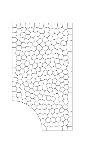
The geometric data are
We consider a plasticity model with linear kinematic and isotropic hardenings (see for instance [27]) with material parameters
For comparison purposes, we take as “exact solution” one obtained with linear finite elements on a fine triangular mesh with elements. Note that, since the considered model includes hardenings, there is no risk of volumetric locking and thus triangular elements are a good choice. We solve the problem on a sequence of four Voronoi meshes (mesh V1 to mesh V4) generated with the code PolyMesher [29]. We depict a sample mesh V2 in figure 3 (right) while the number of vertices in each grid can be found in Table 5. In all cases we use the incremental loading procedure described in Section 3.3 with 100 time-steps. At each time step the constitutive law is solved using a classical radial return map algorithm (see for instance [27], Chapter 3). For each mesh we show the following values in Table 5:
-
•
The vertical displacement at the point A of coordinates , where the axes origin is at the center of the hole;
-
•
the horizontal displacement at the point B of coordinates ;
-
•
the maximum stress ;
-
•
the total stress , i.e. the integral over of the stress amplitude .
| Mesh | Displ. A | Displ. B | |||
|---|---|---|---|---|---|
| V1 | 129 | 0.7839 | -0.3181 | 3.3842 | 244.2324 |
| V2 | 511 | 0.8173 | -0.3928 | 4.1354 | 240.1062 |
| V3 | 2032 | 0.8253 | -0.4212 | 4.4266 | 238.7653 |
| V4 | 8131 | 0.8277 | -0.4300 | 4.7755 | 238.3688 |
| Reference | 22921 | 0.8284 | -0.4334 | 4.9891 | 238.2631 |
Note that, on purpose, in Table 5 we consider quantities for which is easy to obtain convergence (displacement at point A ad total stress) and other ones for which is harder (displacement at point B and maximum stress). In all cases we can appreciate the convergence of the method towards the reference values; finer Voronoi meshes would be needed for a better approximation of the maximum stress.
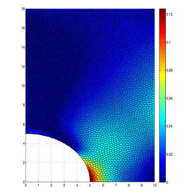
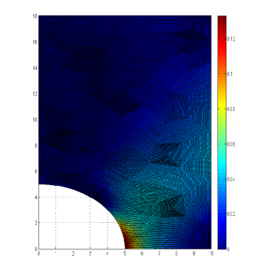
In figure 4 we depict the value of the plastic consistency parameter for the V4 and for the fine reference mesh. The parameter indicates if and how much plastification has occurred locally for the material; we refer again to [27] for a detailed description of the model. Again, the results for the proposed method are in good accordance with the reference one.
5.4 Finite strain elasticity
The method detailed in Sections 3.1-3.2 can also be applied to elastic problems in a large strain regime. However, we remark that the complexity of the finite elasticity problem requires a much deeper design and analysis than the one here presented. Therefore, the following discussion should be intended only as a very preliminary study towards the VEM discretization of large deformation elastic problems.
We here focus on neo-Hookean hyperelastic materials, but different constitutive laws could be considered. Following a material description (see [9, 15, 25], for instance), the variational formulation of the elastic large deformation problem reads as in (3):
| (56) |
where the first Piola-Kirchhoff stress tensor is not necessarily symmetric. As for Problem (3), in (56) the symbol denotes the space of admissible displacements and the space of its variations. A homogeneous neo-Hookean material is described by the constitutive law:
| (57) | ||||
Above, and are given constants, is a suitable smooth function, and is defined as
| (58) |
Here, we choose , so that .
A possible virtual method for Problem (56) can be designed exactly as in Sections 3.1-3.2 , simply by systematically substituting in place of .
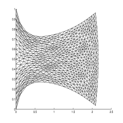
We test the method considering a square block of side length , which initially occupies the region . We impose clamped boundary conditions on the side , while the remaining part of the boundary is free. The material parameters are chosen as and . The load is given by .
Table 6 displays the computed displacements of the material point , when using triangular (T1,…,T4), quadrilateral (Q1,…,Q4), and hexagonal Voronoi (V1,…,V4) meshes. A reference solution at the same point, obtained with a very fine triangular mesh of elements, corresponding to mesh vertices, is also reported. Finally, Figure 5 depicts the deformed body when using the triangular mesh T2, the square mesh Q2 and the hexagonal Voronoi mesh V2 of Table 6. We notice that for every considered scheme, convergence to the reference solution occurs, and the deformed shapes appear to be sensible.
| Mesh | Displ. at | Displ. at | |
|---|---|---|---|
| T1 | 55 | 0.9865 | -0.0438 |
| T2 | 183 | 1.0615 | -0.0398 |
| T3 | 727 | 1.0848 | -0.0358 |
| T4 | 2810 | 1.0967 | -0.0354 |
| Q1 | 49 | 0.9979 | -0.0736 |
| Q2 | 196 | 1.0730 | -0.04791 |
| Q3 | 784 | 1.0950 | -0.0391 |
| Q4 | 3025 | 1.1005 | -0.0364 |
| V1 | 52 | 0.9125 | -0.0673 |
| V2 | 199 | 1.0344 | -0.0520 |
| V3 | 800 | 1.0722 | -0.0408 |
| V4 | 3179 | 1.0918 | -0.0368 |
| Reference | 35459 | 1.1018 | -0.0353 |
6 Conclusions
We have presented a Virtual Element Method to deal with fairly general non-linear elastic and inelastic problems. Our scheme is based on a low-order approximation of the displacement field, together with a suitable treatment of the numerical displacement gradient. The proposed method allows for general polygonal/polyhedral meshes, is efficient in terms of number of applications of the constitutive law, and can make use of any standard black-box constitutive law algorithm. We have presented several numerical tests assessing the computational performance of the proposed methodology. However, we remark that this study is intended as a first step towards the design of efficient Virtual Element Methods for non-linear Computational Mechanics problems. Many possible extensions and improvements could be of interest. For instance, large deformation problems require a much deeper investigations, and other inelastic cases such as perfect plasticity or damage could be considered.
Acknowledgements. D. Mora was partially supported by CONICYT-Chile through FONDECYT project No. 1140791 and by project Anillo ACT 1118 (ANANUM).
References
- [1] B. Ahmed, A. Alsaedi, F. Brezzi, L.D. Marini, and A. Russo. Equivalent Projectors for Virtual Element Methods. Comput. Math. Appl., 66(3):376–391, 2013.
- [2] L. Beirão da Veiga, F. Brezzi, A. Cangiani, G. Manzini, L. D. Marini, and A. Russo. Basic principles of Virtual Element Methods. Math. Models Methods Appl. Sci., 23:119–214, 2013.
- [3] L. Beirão da Veiga, F. Brezzi, and L. D. Marini. Virtual Elements for linear elasticity problems. SIAM J. Numer. Anal., 51:794–812, 2013.
- [4] L. Beirão da Veiga, F. Brezzi, L. D. Marini, and A. Russo. The Hitchhikers Guide to the Virtual Element Method. Math. Models Methods Appl. Sci., 24(8):1541–1573, 2014.
- [5] L. Beirão da Veiga, K. Lipnikov, and G. Manzini. The Mimetic Finite Difference Method for Elliptic Problems. Springer, series MS&A (vol. 11), 2014.
- [6] L. Beirão da Veiga and G. Manzini. A Virtual Element Method with arbitrary regularity. IMA J. Numer. Anal., 34(2):759–781, 2014.
- [7] S. Biabanaki, A. Khoei, and P. Wriggers. Polygonal finite element methods for contact-impact problems on non-conformal meshes. Comp. Meth. Appl. Mech. Engrng., 269:198–221, 2014.
- [8] D. Boffi, F. Brezzi, and M. Fortin. Mixed Finite Element Methods and Applications. Springer-Verlag, Berlin Heidelberg, 2013.
- [9] J. Bonet and R.D. Wood. Nonlinear Continuum Mechanics for Finite Element Analysis. Cambridge University Press; 2 edition, 2008.
- [10] F. Brezzi, K. Lipnikov, and M. Shashkov. Convergence of the mimetic finite difference method for diffusion problems on polyhedral meshes. SIAM J. Numer. Anal., 43(5):1872–1896, 2005.
- [11] F. Brezzi and L.D. Marini. Virtual Element Method for plate bending problems. Comput. Methods Appl. Mech. Engrg., 253:455–462, 2012.
- [12] Talischi C., Paulino G.H., Pereira A., and Menezes I.F.M. Polygonal finite elements for topology optimization: A unifying paradigm. Int. J. for Num. Meth. Engnr., 82:671–698, 2010.
- [13] H. Chi, C. Talischi, O. Lopez-Pamies, and G.H. Paulino. Polygonal finite elements for finite elasticity. Int. J. Numer. Meth. Engrg., 101(4):305–328, 2015.
- [14] P. G. Ciarlet. The Finite Element Method for Elliptic Problems. North-Holland, Amsterdam, 1978.
- [15] P.G. Ciarlet. Mathematical Elasticity: Three-dimensional elasticity, Volume 1. Elsevier, 1993.
- [16] B. Cockburn, J. Gopalakrishnan, and R. Lazarov. Unified hybridization of discontinuous Galerkin, mixed, and continuous Galerkin methods for second order elliptic problems. SIAM J. Numer. Anal., 47(2):1319–1365, 2009.
- [17] D. Di Pietro and A. Alexandre Ern. A hybrid high-order locking-free method for linear elasticity on general meshes. Comput. Methods Appl. Mech. Engrg., 283(0):1–21, 2015.
- [18] D. Di Pietro and A. Ern. Hybrid high-order methods for variable-diffusion problems on general meshes. In press, 2014.
- [19] M. Floater, A. Gillette, and N. Sukumar. Gradient bounds for Wachspress coordinates on polytopes. SIAM J. Numer. Anal., 52(1):515–532, 2014.
- [20] A.L. Gain, G.H. Paulino, L. Duarte, and I.F.M. Menezes. Topology Optimization Using Polytopes. Preprint arXiv:1312.7016. Submitted for publication.
- [21] A.L. Gain, C. Talischi, and G.H. Paulino. On the Virtual Element Method for Three-Dimensional Elasticity Problems on Arbitrary Polyhedral Meshes. Comp. Meth. Appl. Mech. Engrg., 282:132–160, 2014.
- [22] G.N. Gatica, A. Márquez, and W. Rudolph. A priori and a posteriori error analyses of augmented twofold saddle point formulations for nonlinear elasticity problems. Comp. Meth. Appl. Mech. Engrng., 264,:23–48, 2013.
- [23] W. Han and B.D. Reddy. Plasticity. Mathematical Theory and Numerical Analysis. Springer-Verlag New York, 2013.
- [24] S.E. Leon, D. Spring, and G.H. Paulino. Reduction in mesh bias for dynamic fracture using adaptive splitting of polygonal finite elements. Int. J. Numer. Meth. Engrng., 100:555–576, 2014.
- [25] J.E. Marsden and T.J.R. Hughes. Mathematical Foundations of Elasticity. Dover, 1994.
- [26] D. Mora, G. Rivera, and R. Rodríguez. A virtual element method for the Steklov eigenvalue problem. CI2MA Pre-Publicación 2014-27, in press on Math. Mod. Meth. Appl. Math., 2015.
- [27] J. C. Simo and T. J. R. Hughes. Computational Inelasticity. Springer-Verlag New York, 1998.
- [28] N. Sukumar and A. Tabarraei. Conforming polygonal finite elements. Int. J. Numer. Meth. Engrg., 61:2045–2066, 2004.
- [29] C. Talischi, G.H. Paulino, A. Pereira, and I.F.M. Menezes. PolyMesher: a general-purpose mesh generator for polygonal elements written in Matlab. Structural and Multidisciplinary Optimization, 45(3):309–328, 2012.
- [30] J. Wang and X. Ye. A weak Galerkin finite element method for second-order elliptic problems. J. Comput. Appl. Math., 241:103–115, 2013.
- [31] J. Wang and X. Ye. A weak Galerkin mixed finite element method for second order elliptic problems. Math. Comp., 83(289):2101–2126, 2014.