Abstract

The Totally Asymmetric Simple Exclusion Process (TASEP) is a non-equilibrium particle model on a finite one-dimensional lattice with open boundaries. In our earlier paper, we obtained a determinantal formula that computes the steady state probabilities of this process by the enumeration of “Catalan alternative tableaux”, which are certain fillings of Young diagrams. Here, we present a new, more illuminating bijective proof of this determinantal formula using the Lindström-Gessel-Viennot Lemma.

1 The TASEP and Catalan alternative tableaux

The totally asymmetric exclusion process (TASEP) is a version of the well-studied non-equilibrium particle model from statistical mechanics. In a TASEP of size $n$, particles hop to the right along a line with locations labelled 1 through $n$ such that there is at most one particle per location, and particles can enter at location 1 and exit from location $n$ with respective rates $\alpha$ and $\beta$. A state of the TASEP is described by a word $\tau=\tau_{1}\ldots\tau_{n}$ in $\{0,1\}^{n}$ where $\tau_{i}=1$ if there is a particle in location $i$, and $\tau_{i}=0$ otherwise. The discrete Markov process can be defined as follows, for $\tau^{\prime}$ and $\tau^{\prime\prime}$ arbitrary words in $\{0,1\}^{\ast}$: at each time step,

$$0\tau^{\prime}\overset{\alpha}{\rightharpoonup}1\tau^{\prime}\qquad\tau^{\prime}1\overset{\beta}{\rightharpoonup}\tau^{\prime}0\qquad\tau^{\prime}10\tau^{\prime\prime}\overset{1}{\rightharpoonup}\tau^{\prime}01\tau^{\prime\prime}$$

where $X\overset{p}{\rightharpoonup}Y$ means that the transition from $X$ to $Y$ occurs with probability $\frac{p}{n+1}$ where $n$ is the length of $X$ and $Y$. We use the notation $Pr(\tau)$ to denote the stationary probability of state $\tau$.

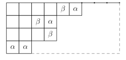
Figure 1: A Catalan tableau of size $(13,4)$, type 0001001100100, and weight $\alpha^{8}\beta^{12}$.

A large number of related combinatorial objects interpret the stationary probabilities of the TASEP, and an explicit determinantal formula was given in [4] for $\Pr(\tau)$. In this work, we present a simple bijective proof for that formula that uses the Lindström-Gessel-Viennot Lemma. We begin by defining the main object, the Catalan alternative tableau.

Definition 1.1.

A Catalan alternative tableau $T$ of size $(n,k)$ is a Young diagram $Y=Y(T)$ contained in a $k\times n-k$ rectangle, justified to the northwest, together with a filling of the boxes of $Y$ with $\alpha$’s and $\beta$’s according to the following rules:

1. Every box in the same column and above an $\alpha$ must be empty.

2. Every box in the same row and left of a $\beta$ must be empty.

3. Every box that does not lie above an $\alpha$ or left of a $\beta$ must contain an $\alpha$ or a $\beta$.

We associate to $T$ a lattice path $L=L(T)$ with steps south and west, which starts at the northeast corner of the rectangle and ends at the southwest corner, and follows the southeast border of $Y$. The type of $T$ is the word $\tau$ in $\{0,1\}^{\ast}$ that we obtain by reading $L$ from northeast to southwest and assigning a 1 to a south-step and a 0 to a west-step.

We also associate to $Y$ the partition $\lambda=\lambda(T)=(\lambda_{1},\ldots,\lambda_{k})$, where $\lambda_{1}\geq\lambda_{2}\geq\cdots\geq\lambda_{k}\geq 0$ and $\lambda_{i}$ is the number of boxes in $Y$ in the $i$th row of the rectangle. We call $\lambda$ the shape of $T$ and of $Y$.

Definition 1.2.

For a Catalan alternative tableau $T$ with associated shape $\lambda(T)$ and of type $\tau$ with exactly $k$ 1’s, we make the equivalent definition $\lambda(\tau)=(\lambda_{1},\ldots,\lambda_{k})$. Here $\lambda_{i}$ is the number of 0’s following the $i$’th 1 in the word $\tau$. It is easy to see that $\lambda(T)=\lambda(\tau)$.

Definition 1.3.

For a Catalan alternative tableau $T$ of size $(n,k)$ and its associated Young diagram $Y$, an $\alpha$-free column is a column of the $k\times n-k$ rectangle containing $Y$ that does not contain an $\alpha$. Similarly, a $\beta$-free row is a row of the rectangle that does not contain a $\beta$.

Definition 1.4.

The weight of a Catalan alternative tableau $T$ of size $(n,k)$ with associated Young diagram $Y$ is

$$\operatorname{wt}(T)=(\alpha\beta)^{n}\left(\frac{1}{\alpha}\right)^{\operatorname{f\,col}(T)}\left(\frac{1}{\beta}\right)^{\operatorname{f\,row}(T)}$$

where $\operatorname{f\,col}(T)$ is the number of $\alpha$-free columns and $\operatorname{f\,row}(T)$ is the number of $\beta$-free rows in $T$.

Example.

Figure 1 shows a Catalan alternative tableau of type 0001001100100, weight $\alpha^{8}\beta^{12}$ with $\lambda(T)=(6,4,4,2)$.

Catalan alternative tableaux are a specialization of “alternative tableaux”, which are more general objects connected to the combinatorics of the PASEP (an exclusion process in which particles are allowed to hop both left and right). The alternative tableaux are related by simple bijections to several similar objects in the literature, such as permutation tableaux, staircase tableaux, and tree-like tableaux. Some references for these objects can be found in [9, 10] (thus we could similarly define Catalan permutation tableaux, Catalan staircase tableaux, and Catalan tree-like tableaux). Furthermore, connections to the combinatorics of the (P)ASEP are explored in an expansive collection of slides from lectures given by Viennot in [7]. The author recommends these slides and references therein as a source for further reading on this topic. For the rest of this paper, we will refer to the Catalan alternative tableaux simply as “Catalan tableaux”.

Theorem 1.1.

Let $\tau$ be a word in $\{0,1\}^{n}$ with $k$ 1’s representing a state of the TASEP of length $n$ with exactly $k$ particles. Let $\lambda(\tau)=(\lambda_{1},\ldots,\lambda_{k})$ be the partition associated to $\tau$. Define $P(\tau)=\sum_{T}wt(T)$ where the sum is over Catalan tableaux $T$ of type $\tau$. Then

$$P(\tau)=\alpha^{k+\lambda_{1}}\beta^{n}\det A^{\alpha,\beta}_{\lambda(\tau)}$$

where $A^{\alpha,\beta}_{\lambda(\tau)}=(A_{ij})_{1\leq i,j\leq k}$ with

$$A_{ij}=\left({\lambda_{j+1}\choose j-i+1}+\frac{1}{\beta}{\lambda_{j+1}\choose j-i}\right)+\sum_{p=1}^{\lambda_{j}-\lambda_{j+1}}\left(\frac{1}{\alpha}\right)^{p}\left({\lambda_{j+1}+p-1\choose j-i}+\frac{1}{\beta}{\lambda_{j+1}+p-1\choose j-i-1}\right).$$

We give the proof in Section 3.1. Instead, here we demonstrate the importance of the above in connection with the TASEP. From the following theorem, we obtain that $P(\tau)$ plays a central role in computing the stationary probability of state $\tau$ of the TASEP.

Theorem 1.2 (Corteel, Williams (2007)).

Let $Z_{n}=\sum_{T^{\prime}}wt(T^{\prime})$ be the sum of the weights of all Catalan tableaux $T^{\prime}$ of size $n$. Then

$$Pr(\tau)=\frac{1}{Z_{n}}\sum_{T}wt(T)$$

where the sum is over Catalan tableaux $T$ of type $\tau$.

Furthermore, from Derrida et. al. [3], we have the following formula.

$$Z_{n}=(\alpha\beta)^{n}\sum_{p=1}^{n}\frac{p}{2n-p}{2n-p\choose n}\frac{\alpha^{-p-1}-\beta^{-p-1}}{\alpha^{-1}-\beta^{-1}}.$$ (1.1)

Thus we obtain the final result.

Corollary 1.3.

The stationary probability of state $\tau$ of a TASEP of size $n$ is

$$Pr(\tau)=\frac{\alpha^{k+\lambda_{1}}\beta^{n}}{Z_{n}}\det A^{\alpha,\beta}_{\lambda}.$$

where $\lambda=\lambda(\tau)$ and $Z_{n}$ is of Equation 1.1.

Proof.

The Corollary follows immediately from Theorem 1.1 and Theorem 1.2. ∎

2 Bijection from Catalan tableaux to weighted Catalan paths

In this section, we present a canonical bijection from a filling of the Catalan tableau with associated Young diagram $Y$ to a lattice path on a Young diagram of the same shape. Viennot describes an analogous bijection from Catalan permutation tableaux (which are in bijection to the Catalan tableaux) to weighted lattice paths in [6]. We reformulate this bijection for the Catalan tableaux and assign the weights to the resulting lattice path in a particular way.

2.1 Weighted Catalan path

Let $Y$ be a Young diagram contained within a $k\times n-k$ rectangle. A lattice path constrained by $Y$ is a path that begins in the northeast corner and ends at the southwest corner of rectangle, and takes the steps south and west in such a way that it never crosses the southeast boundary of $Y$.

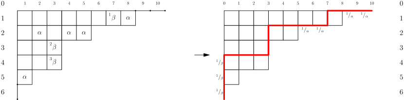
Figure 2: A Catalan tableau $T$ and its corresponding weighted Catalan path $C$ on a tableau of shape $\lambda=(8,5,3,3,1,0)$ and weight $\operatorname{wt}(T)=\alpha^{12}\beta^{13}$. On the left, the $\beta$’s are labeled such as to generate the partition $(7,3,3,0,0,0)$ where the column containing the $i$th beta is the length of the $i$th row of the partition. This partition is precisely the shape of the path in the figure on the right. The path weight of $C$ is $\operatorname{p\,wt}(C)=\left(\frac{1}{\beta}\right)^{3}\left(\frac{1}{\alpha}\right)^{4}$, and so $\operatorname{wt}(C)=(\alpha\beta)^{16}\left(\frac{1}{\beta}\right)^{3}\left(\frac{1}{\alpha}\right)^{4}=\operatorname{wt}(T)$.

Definition 2.1.

A Catalan path $C$ of size $(n,k)$ with associated Young diagram $Y$ is a lattice path constrained by $Y$ with the following weights on its edges:

• A south edge that coincides with the east border of the rectangle receives a $\frac{1}{\beta}$.

• A south edge that does not coincide with the east border of the rectangle receives a 1.

• A west edge that coincides with the south boundary of Y receives a $\frac{1}{\alpha}$.

• A west edge that does not coincide with the south boundary of Y receives a 1.

Definition 2.2.

The path weight $\operatorname{p\,wt}(C)$ of the Catalan path $C$ is the product of the weights on its edges. We call the total weight of the Catalan path $\operatorname{wt}(C)$, with $\operatorname{wt}(C)=(\alpha\beta)^{n}\operatorname{p\,wt}(C)$.

The following lemma describes a natural correspondence between the Catalan tableaux and the Catalan paths.

Lemma 2.1.

There is a weight-preserving bijection between the set of Catalan paths of size $(n,k)$ constrained by the Young diagram $Y$ to the set of Catalan tableaux of size $(n,k)$ of type $\tau$ such that $\lambda(\tau)$ is the same partition that describes $Y$.

Proof.

Let a Catalan path $C$ of size $(n,k)$ constrained by a Young diagram $Y$ of shape $\lambda=(\lambda_{1},\ldots,\lambda_{k})$ be described by the partition $(C_{1},\ldots,C_{k})$ that is weakly smaller than $\lambda$. In other words, $C_{1}\geq C_{2}\cdots\geq C_{k}$ and $0\leq C_{i}\leq\lambda_{i}$, and $C_{i}$ is the position of the south step of the lattice path that occurs in row $i$ of the $k\times n-k$ rectangle.

We map $(C_{1},\ldots,C_{k})$ to a Catalan tableau $T$ as follows. First we label the columns of the $k\times n-k$ rectangle with 1 through $n-k$ from left to right. Then, for $i$ in $\{1,\ldots,k\}$, if $C_{i}>0$, we place a $\beta$ in column $C_{i}$ of $Y$ such that it is the south-most position possible with the condition that there is at most one $\beta$ per row. We now place an $\alpha$ in the lowest possible $\beta$-free row of every column. (Consequently, a column does not receive an $\alpha$ if and only if it has zero $\beta$-free rows.) It is easy to check that this construction results in a valid Catalan tableau.

Conversely, to map a Catalan tableau $T$ to the partition $(C_{1},\ldots,C_{k})$, we label the $\beta$’s in the filling of $Y$ from left to right and top to bottom with $1,\ldots,\ell$ where $\ell$ is the number of $\beta$’s, and we let $C_{i}$ be the label of the column containing the $i$’th beta. We let $C_{\ell+1}=\cdots=C_{k}=0$. In this construction, the labels on the $\beta$’s decrease as the labels on the columns decrease, as in the left image of Figure 2, so $C_{i}\geq C_{i+1}$. The partition $(C_{1},\ldots,C_{k})$ is then directly mapped to the Catalan path $P$.

Now we show the weight $\operatorname{wt}(C)$ of the Catalan path $C$ is the same as the weight $\operatorname{wt}(T)$ of the Catalan tableau $T$. Let $\{C_{i_{1}},\ldots,C_{i_{m}}\}$ be the subset of $\{C_{1},\ldots,C_{k}\}$ that represents the south steps that touch the south boundary of $Y$. Then the contribution of the $\left(\frac{1}{\alpha}\right)$ to the weight of the path is $\prod_{j=1}^{m}\left(\frac{1}{\alpha}\right)^{C_{i_{j}}-\lambda_{i_{j}+1}}$. This is because, for each $j$, if $C_{i_{j}}$ touches the south boundary of $Y$, we know that there are zero $\beta$-free rows in the column $i_{j}$. In particular, no column of the Catalan tableau between $\lambda_{i_{j}+1}$ and $i_{j}$ can contain an $\alpha$, so every west-edge of the path in those columns carries a weight of $\frac{1}{\alpha}$. It follows that both the Catalan tableau and the Catalan path have the same power of $\frac{1}{\alpha}$ contributed to their weight.

As for the factor of $\frac{1}{\beta}$, by the construction of the path, it must be $\left(\frac{1}{\beta}\right)^{t}$, where $t$ is the number of $C_{j}$ that equal 0. But we already know that if $C_{j}=0$, it means that row $j$ of the Catalan tableau is $\beta$-free, and so contributes a $\frac{1}{\beta}$ to the weight of the tableau. Thus $\operatorname{wt}(C)=\operatorname{wt}(T)=(\alpha\beta)^{n}\left(\frac{1}{\beta}\right)^{t}\prod_{j=1}^{m}\left(\frac{1}{\alpha}\right)^{C_{i_{j}}-\lambda_{i_{j}+1}}$ where $t,i_{1},\ldots,i_{m}$ were defined in the above paragraphs. ∎

3 Bijection from a weighted lattice path on a Young diagram of $k$ rows to $k$ disjoint weighted paths

Let $D$ be a digraph where we assume finitely many paths between any two vertices. Let $\textbf{e}=(e_{1},\ldots,e_{k})$ and $\textbf{v}=(v_{1},\ldots,v_{k})$ be $k$-tuples of vertices of $D$. Let every edge of $D$ be assigned a weight.

Definition 3.1.

A $k$-path from e to v is a $k$-tuple of paths $\textbf{P}(\textbf{e},\textbf{v})=(P_{1},\ldots,P_{k})$ where for some fixed $\pi\in S_{k}$, $P_{i}$ is a path from $e_{i}$ to $v_{\pi(i)}$. The $k$-path P is disjoint if the paths $P_{i}$ are all vertex disjoint.

Definition 3.2.

The weight $\operatorname{wt}(P_{i})$ of a path $P_{i}$ is the product of the weights on its edges. The weight $\operatorname{wt}(\textbf{P})$ of the $k$-path $\textbf{P}=(P_{1},\ldots,P_{k})$ is the sum of the weights of its components, in other words $\operatorname{wt}(\textbf{P})=\sum_{i=1}^{k}\operatorname{wt}(P_{i})$.

Theorem 3.1 (Lingström, Gessel-Viennot).

Let $D$ be a digraph, and let $\textbf{u}=(u_{1},\ldots,u_{k})$ and $\textbf{y}=(y_{1},\ldots,y_{k})$ be $k$-tuples of vertices of $D$. Let $\mathcal{P}_{ij}$ be the set of paths from $u_{i}$ to $y_{j}$. Define $w_{ij}=\sum_{p\in\mathcal{P}_{ij}}\operatorname{wt}(p)$. Then

$$\sum_{\pi\in S_{k}}\sum_{\textbf{P}}\operatorname{sgn}(\pi)\operatorname{wt}(\textbf{P})=\det\left(w_{ij}\right)_{1\leq i,j\leq k}.$$

where P ranges over all disjoint $k$-paths $\textbf{P}(\textbf{u},\pi(\textbf{y}))$.

In this section, we provide a bijection from a Catalan path on a Young diagram $Y$ to a disjoint $k$-path on a corresponding digraph with appropriately assigned weights on the edges. Ignoring the weights, we obtain the canonical bijection from lattice paths constrained by a Young diagram to disjoint $k$-paths. This bijection allows us to enumerate the Catalan paths as an application of the Lindström-Gessel-Viennot Lemma.

Let $C$ be a Catalan path of size $(n,k)$ with associated Young diagram $Y$ of shape $\lambda=(\lambda_{1},\ldots,\lambda_{k})$. We label the vertical lines in the $k\times n-k$ rectangle from left to right with $\{0,1,\ldots\,n-k\}$. Let $C$ be described by the partition $(C_{1},\ldots,C_{k})$ where $C_{i}$ is the label of the south-step of $C$ in row $i$. Since $C$ consists of only south- and west- steps, we necessarily have $C_{1}\geq\cdots\geq C_{k}\geq 0$.

Now we define a twisted tableau $\tilde{Y}$ from $Y$ as follows: for $1\leq i\leq k$, draw a row of $\lambda_{i}$ parallelograms consisting of east and southeast edges, and left-justify the rows as in the middle image of Figure 3. In each row, we label the southeast edges of the parallelograms with $0,1,2,\ldots$ from left to right. We put weights on the edges of the parallelograms in the following way:

• the edges with label 0 receive a $\frac{1}{\beta}$,

• otherwise if an edge in row $i$ has label $t$ and $t>\lambda_{i+1}$, the edge receives a $\left(\frac{1}{\alpha}\right)^{t-\lambda_{i+1}}$.

Every other edge receives a weight of 1.

We mark the left-most vertices of each row of parallelograms as the $k$ special points $e_{1},\ldots,e_{k}$ from top to bottom. We also mark the right-most vertices of each row of parallelograms as the $k$ special points $v_{1},\ldots,v_{k}$. Finally, we convert $\tilde{Y}$ into a digraph by directing all its edges from northwest to southeast. We denote by $\mathcal{P}_{ij}$ the set of weighted paths from $e_{i}$ to $v_{j}$.

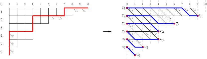
Figure 3: A Catalan path represented by partition $(7,3,3,0,0,0)$ on a Young Diagram with rows $(C_{1},\ldots,C_{6})=(1,\ldots,6)$ and the corresponding set of paths $\{p_{ii}\}_{1\leq i\leq 6}$ where $p_{ii}\in\mathcal{P}_{ii}$ has a single diagonal step at edge labeled $C_{i}$. This Catalan path is the same one as in Figure 2.

We map the partition $(C_{1},\ldots,C_{k})$ on $Y$ to a $k$-path $\textbf{P}(C)=\textbf{P}(\textbf{e},\textbf{v})$ on $\tilde{Y}$ in the following way. We write $\textbf{P}(C)=(p_{11},\ldots,p_{kk})$ where $p_{ii}\in\mathcal{P}_{ii}$. For each $i$ in $\{1,\ldots,k\}$, we define $p_{ii}$ as follows: let the single diagonal step in $p_{ii}$ be the southeast edge in row $i$ with label $C_{i}$. The rest of the edges in $p_{ii}$ must necessarily be the horizontal edges that connect that diagonal step from $e_{i}$ to $v_{i}$. From Figure 3, it is easy to see this is a one to one correspondence.

Remark 3.1.

It is important to note that the segment of $C$ that lies in the columns $\{\lambda_{1}+1,\ldots,n-k\}$ is ignored in the construction of $\textbf{P}(C)$. This is permissible since any Catalan path constrained by $\lambda$ must necessarily have the same such segment. Thus it suffices to simply adjust the weight of $\textbf{P}(C)$ by the weight contribution of that segment, which is $\left(\frac{1}{\alpha}\right)^{n-k-\lambda_{1}}$.

Lemma 3.2.

Based on the construction of the $k$-path $\textbf{P}(C)$ above, we claim that (i.) $\textbf{P}(C)$ is disjoint if and only if $C_{1}\geq\cdots\geq C_{k}$ and (ii.) $\operatorname{p\,wt}(C)=\left(\frac{1}{\alpha}\right)^{n-k-\lambda_{1}}\operatorname{wt}(\textbf{P}(C))$.

Proof.

[i.] It is easy to see from the construction that $C_{i}\geq C_{i+1}$ if and only if the diagonal edge in row $i$ is strictly to the right of the diagonal edge in row $i+1$. That implies $p_{ii}$ is strictly to the northeast of $p_{i+1\ i+1}$. Since the $p_{ii}$’s are nested paths, this implies $\textbf{P}(C)$ is disjoint.

[ii.] We prove the equality by comparing $\operatorname{wt}(p_{ii})$ to the weight contribution of the segment of $C$ that is in row $i$ (including the south border of the row), and showing they are equal for each $1\leq i\leq k$.

• First, if $C_{i}=0$, then $\operatorname{wt}(p_{ii})=\frac{1}{\beta}$, and also the weight contribution of row $i$ in $C$ is $\frac{1}{\beta}$. See rows 3-6 in the example in Figure 3.

• When $C_{i}>0$, there is no contribution of $\frac{1}{\beta}$ to the segment of $C$ in row $i$ or to $p_{ii}$, so we consider only the contribution of $\frac{1}{\alpha}$. If $0<C_{i}\leq\lambda_{i+1}$, the south-step of $C$ in row $i$ does not touch the south boundary of $Y$, so there is no contribution of $\frac{1}{\alpha}$ from that segment of the path, and hence the total weight contribution is 1. Similarly, $p_{ii}$ does not contain any edges with non-unit weight and so $\operatorname{wt}(p_{ii})=1$. See rows 2-3 in the example in Figure 3.

• If $C_{i}>\lambda_{i+1}$, the south-step of $C$ in row $i$ touches the south boundary of $Y$, so that segment of the path has $C_{i}-\lambda_{i+1}$ west-edges that coincide with the south boundary of $Y$ and thus carry the weight $\frac{1}{\alpha}$. Thus the total contribution to the weight of the segment of $C$ in row $i$ is $\left(\frac{1}{\alpha}\right)^{C_{i}-\lambda_{i+1}}$. By the construction, $p_{ii}$ has weight $\left(\frac{1}{\alpha}\right)^{C_{i}-\lambda_{i+1}}$ on its diagonal edge, and that also equals $\operatorname{wt}(p_{ii})$. See row 1 in the example in Figure 3.

From the above, for each $i$, the contribution of the weight of the segment of $C$ in row $i$ equals $\operatorname{wt}(p_{ii})$. By Remark 3.1, we have excluded from $\textbf{P}(C)$ the contribution of the weight of the segment of $C$ that lies to the northeast of $Y$. Consequently, we have $\operatorname{p\,wt}(C)=\left(\frac{1}{\alpha}\right)^{n-k-\lambda_{i}}\operatorname{wt}(\textbf{P}(C))$ as desired. ∎

3.1 Proof of Theorem 1.1

We make the simple observation that a $k$-path $(P_{i},\ldots,P_{k})$ from the e to v is disjoint if and only if each path $P_{i}$ is from $e_{i}$ to $v_{i}$. As before, let $w_{ij}=\sum_{p\in\mathcal{P}_{ij}}\operatorname{wt}(p)$ for $\mathcal{P}_{ij}$ the collection of paths from $e_{i}$ to $v_{j}$. Then from the bijection above and from Theorem 3.1, we obtain

$$\sum_{C}\operatorname{p\,wt}(C)=\left(\frac{1}{\alpha}\right)^{n-k-\lambda_{i}}\sum_{\textbf{P}}\operatorname{wt}(\textbf{P})=\left(\frac{1}{\alpha}\right)^{n-k-\lambda_{i}}\det\left(w_{ij}\right)_{1\leq i,j\leq k},$$

where $C$ ranges over the Catalan tableaux constrained by $Y$, and P ranges over the disjoint $k$-paths from e to v on $\tilde{Y}$.

It is not difficult to check that $w_{ij}$ for $i,j>0$ equals precisely the entry $A_{ij}$ from Theorem 1.1. We describe the calculations below.

Consider the paths from $e_{i}$ to $v_{j}$ that have weight generating function $w_{ij}$. First, if $i>j+1$, there are zero such paths since all paths can only take east and southeast steps. Next, if $i=j+1$, there is exactly one path, namely the one that takes only horizontal steps from $e_{i}$, and so the weight on that path is 1, and thus $w_{i,i-1}=1$. Finally, assume $i\leq j$. Then any path in $\mathcal{P}_{ij}$ takes $j-i+1$ southeast steps, of which at most one step could have a weight of $\frac{1}{\beta}$, and at most one other step could have a weight of $\left(\frac{1}{\alpha}\right)^{\ell}$ for some $\ell>0$. Thus we count four cases for paths in $\mathcal{P}_{ij}$:

1. A path has all its steps of weight 1. The path necessarily takes the first step east and goes to the right-most vertex of parallelogram number $\lambda_{i+1}$ in the $i$th row. This can happen in ${\lambda_{i+1}\choose j-i+1}$ ways, and every such path has weight 1.

2. A path has one step of weight $\frac{1}{\beta}$ and the rest of weight 1. The path necessarily takes the first step southeast and goes to the right-most vertex of parallelogram number $\lambda_{i+1}$ in the $i$th row. This can happen in ${\lambda_{i+1}\choose j-i+1}$ ways, and every such path has weight $\frac{1}{\beta}$.

3. A path has one step of weight $\left(\frac{1}{\alpha}\right)^{\ell}$ and the rest of weight 1. The path necessarily takes the first step east and goes to the right-most vertex of parallelogram number $\lambda_{i+1}+\ell-1$ in row $i-1$. This can happen in ${\lambda_{i+1}+\ell\choose j-i}$ ways, and every such path has weight $\left(\frac{1}{\alpha}\right)^{\ell}$, where $1\leq\ell\leq\lambda_{i}-\lambda_{i+1}$.

4. A path has one step of weight $\frac{1}{\beta}$, one step of weight $\left(\frac{1}{\alpha}\right)^{\ell}$, and the rest of weight 1. The path necessarily takes the first step southeast and goes to the right-most vertex of parallelogram number $\lambda_{i+1}+\ell-1$ in row $i-1$. This can happen in ${\lambda_{i+1}+\ell\choose j-i-1}$ ways, and every such path has weight $\frac{1}{\beta}\left(\frac{1}{\alpha}\right)^{\ell}$, where $1\leq\ell\leq\lambda_{i}-\lambda_{i+1}$.

We combine the above to obtain $A_{\lambda}=\left(w_{ij}\right)_{1\leq i,j\leq k}$ as desired.

Finally, if $C$ is the Catalan path corresponding to the Catalan tableau $T$, since $\operatorname{wt}(T)=\operatorname{wt}(C)=(\alpha\beta)^{n}\operatorname{p\,wt}(C)=\beta^{n}\alpha^{k+\lambda_{1}}\operatorname{wt}(\textbf{P}(C))$, we obtain the desired formula.∎

Acknowledgement. The author gratefully acknowledges Xavier G. Viennot for enlightening conversations that inspired this work.

References

- [1] S. Corteel and L. Williams. Tableaux combinatorics for the asymmetric exclusion process, Advances in Applied Mathematics, Volume 39, Issue 3, 293–310 (2007).
- [2] S. Corteel and L. Williams. Tableaux combinatorics for the asymmetric exclusion process and Askey-Wilson polynomials. Duke Math. J., 159: 385–415, (2011).
- [3] B. Derrida, M. Evans, V. Hakim, V. Pasquier. Exact solution of a 1D asymmetrix exclusion model using a matrix formulation, J. Phys. A: Math. Gen. 26, 1493–1517 (1993).
- [4] O. Mandelshtam. A Determinantal Formula for Catalan Tableaux and TASEP Probabilities, J. Combin. Theory Ser. A (2015).
- [5] E. Duchi and G. Schaeffer. A combinatorial approach to jumping particles, J. Combin. Theory Ser. A 110, 1–29 (2005).
- [6] X. G. Viennot. Canopy of binary trees, Catalan tableaux and the asymmetric exclusion process, FPSAC 2007, Formal Power Series and Algebraic Combinatorics (2007).
- [7] X. G. Viennot. Alternative tableaux, permutations and partially asymmetric exclusion process. Workshop “Statistical Mechanics and Quantum-Field Theory Methods in Combinatorial Enumeration”, Isaac Newton Institute for Mathematical Science, Cambridge, 23 April 2008, video and slides available at: http://sms.cam.ac.uk/media/1004.
- [8] X. G. Viennot. Forme des permutations, chemins et profil des arbres binaires, 52ème SLC, LascouxFest, Domaine Saint Jacques, Otrott, Mars 2004, slides available at: http://www.xavierviennot.org/xavier/exposes_files/LascouxFest.pdf.
- [9] P. Nadeau. The structure of alternative tableaux. J. Combin. Theory Ser. A 118, no. 5, 1638–1660 (2011).
- [10] J. Aval, A. Boussicault, P. Nadeau. Tree-like tableaux. Electron. J. Combin. 20, no. 4, Paper 34, 24 pp. (2013).
- [11] I. Gessel, X. G. Viennot. Determinants, Paths and Plane Partitions, Brandeis University, 36p. (1989).