^affil0^affil0affiliationtext: Department of Applied Mathematics and Computer Science, Technical University of Denmark, DK-2800 Kgs. Lyngby, Denmark.

Tomographic Image Reconstruction using Training Images

Sara Soltani ssol@dtu.dk Martin S. Andersen mskan@dtu.dk Per Christian Hansen pcha@dtu.dk

Abstract

We describe and examine an algorithm for tomographic image reconstruction where prior knowledge about the solution is available in the form of training images. We first construct a nonnegative dictionary based on prototype elements from the training images; this problem is formulated as a regularized non-negative matrix factorization. Incorporating the dictionary as a prior in a convex reconstruction problem, we then find an approximate solution with a sparse representation in the dictionary. The dictionary is applied to non-overlapping patches of the image, which reduces the computational complexity compared to other algorithms. Computational experiments clarify the choice and interplay of the model parameters and the regularization parameters, and we show that in few-projection low-dose settings our algorithm is competitive with total variation regularization and tends to include more texture and more correct edges.

^†^†This work is part of the project HD-Tomo funded by Advanced Grant No. 291405 from the European Research Council^†^†2010 Mathematics Subject Classification: Primary: 65F22; Secondary: 65K10.^†^†Key words and Phrases: Tomography, Dictionary learning, Inverse problem, Regularization, Sparse representation, Image reconstruction.

1 Introduction

Computed tomography (CT) is a technique to compute an image of the interior of an object from measurements obtained by sending X-rays through the object and recording the damping of each ray. CT is used routinely in medical imaging, materials science, nondestructive testing and many other applications.

CT is an inverse problem [MuSi12] and it is challenging to obtain sharp and reliable reconstructions in low-dose measurements where we face underdetermined systems of equations, because we must limit the accumulated amount of X-rays for health reasons or because measurement time is limited. In these circumstances the classic methods of CT, such as filtered back projection [Kuch14] and algebraic reconstruction techniques [HansenHansen], are often incapable of producing satisfactory reconstructions because they fail to incorporate adequate prior information [Bian]. To overcome these difficulties it is necessary to incorporate a prior about the solution that can compensate for the lack of data.

A popular prior is that the image is piecewise constant, leading to total variation (TV) regularization schemes [LaRoque], [Velikina]. These methods can be very powerful when the solution is approximately composed of homogeneous regions separated by sharp boundaries.

An completely different approach is to use prior information in the form of “training images” that characterize the geometrical or visual features of interest, e.g., from high-accuracy reconstructions (the typical case) or from pictures of specimen slices. The goal of this work is to elaborate on this approach. In particular we consider the two-stage framework where the most important features of the training data are first extracted and then integrated in the reconstruction problem.

A natural way to extract and represent prior information from training images is to form a dictionary that sparsely encodes the information [Olshausen]. Learning the dictionary from given training data appears to be very suited for incorporating priors that are otherwise difficult to formulate in a closed form, such as image texture. Dictionary learning — combined with sparse representation [Bruckstein, Eladbook, Tropp] — is now used in many image processing areas including denoising [Chen], [Li], inpainting [Mairal0], and deblurring [Liu]. Elad and Ahron [Elad] address the image denoising problem using a process that combines dictionary learning and reconstruction. They use a dictionary trained from a noise-free image using the K-SVD algorithm [Aharon] combined with an adaptive dictionary trained on patches of the noisy image.

The use of dictionary learning in tomographic imaging has also emerged recently, e.g., in X-ray CT [Etter, Xu, Zhao], magnetic resonance imaging [Huang, Ravishankar], electron tomography [LiuB], positron emission tomography [ChenS], and phase-contrast tomography [Mirone]. Two different approaches have emerged — either one constructs the dictionary from the given data in a joint learning-reconstruction algorithm [ChenS, Huang, LiuB, Ravishankar], or one constructs the dictionary from training images in a separate step before the reconstruction [Etter, Mirone, Xu, Zhao]. Most of these works use K-SVD to learn the dictionary (except [Etter] that uses an “online dictionary learning method” [Mairal1]), and all the methods regularize the reconstruction by means of a penalty that is applied to a patch around every pixel in the image. In other words, all patches in the reconstruction should be close to the subspace spanned by the dictionary images. While all these methods perform better than classical reconstruction methods, they show no significant improvement over the TV-regularized approach.

In simultaneous learning and reconstruction, where the dictionary is learned from the given data, the prior is purely data-driven. Hence, one can argue that it violates a fundamental principle of inverse problems where a data-independent prior is incorporated to eliminate unreasonable models that fit the data. For this reason we prefer to separate the two steps (which requires that reliable training images are available). We describe and examine a two-stage framework where we first construct a dictionary that contains prototype elements from these images, and then we use the dictionary as a prior to regularize the reconstruction problem via computing a solution that has a sparse representation in the dictionary.

Our two-stage algorithm is inspired by the work in [Etter] and, to some extent, [Xu]. The algorithm in [Etter] is tested on a simple tomography setup with no noise in the data and in [Xu] the dictionary is trained from an image reconstructed by a high-dose X-ray exposure and then used to reconstruct the same image with fewer X-ray projections. We utilize the dictionary in a different way using blocks of the image (to be discussed later) which reduces the number of unknowns. We seek to use more realistic simulations with noisy data, we avoid committing “inverse crime,” and we perform a careful study of the sensitivity of the reconstruction to the different parameters in the reconstruction model and in the algorithm. Finally we compare our algorithm with both classical methods and with TV. We are not aware of comprehensive studies of the influence of the learned dictionary structure and dictionary parameters in CT.

Our paper is organized as follows. In section 2 we briefly discuss dictionary learning methods and present a framework for solving the image reconstruction problem using dictionaries, and in Section 3 we describe the implementation details of algorithm. Section 4 presents careful numerical experiments where we study the influence of the algorithm and design parameters. Section LABEL:sec:Final summarizes our work. We use the following notation, where $A$ is an arbitrary matrix:

\textstyle\|A\|_{\mathrm{F}}=\left(\sum_{ij}A_{ij}^{2}\right)^{1/2},\quad\|A\|_{\mathrm{sum}}=\sum_{ij}|A_{ij}|,\quad\|A\|_{\max}=\max_{ij}|A_{ij}|.

2 The Reconstruction Framework

X-ray CT is based on the principle that if we send X-rays through an object and measure the damping of each ray then, with infinitely many rays, we can perfectly reconstruct the object. The attenuation of an X-ray is proportional to the object’s attenuation coefficient, as described by Lambert-Beer’s law [Buzug, §2.3.1]. We divide the domain onto pixels whose unknown nonnegative attenuation coefficients are organized in the vector $x\in\mathbb{R}^{n}$ . Similarly we organize the measured damping of the rays into the vector $b\in\mathbb{R}^{m}$ . Then we obtain a linear system of equations $A\,x=b$ with a large sparse system matrix governed solely by the geometry of the measurements: element $a_{ij}$ is the length of the $i$ th ray passing through pixel $j$ , and the matrix is sparse because each ray only hits a small number of pixels [MuSi12].

The matrix $A$ is ill-conditioned, and often rank deficient, due to the ill-posedness of the underlying inverse problem and therefore the solution is very sensitive to noise in the data $b$ . For this reason, a simple least squares approach with nonnegativity constraints fails to produce a meaningful solution, and we must use regularization to incorporate prior information about the solution [Hansen].

This work is concerned with underdetermined problems where $m<n$ , and the need for regularization is even more pronounced. Classical reconstruction methods such as filtered back projection and algebraic iterative methods are not suited for these problems because they fail to incorporate enough prior information. TV regularization, which is suited for edge-preserving reconstructions, takes the form

\min_{x}\quad{\textstyle\frac{1}{2}}\,\|A\,x-b\|_{2}^{2}+\lambda_{\mathrm{TV}}\sum_{1\leq i\leq n}\left\|D^{\mathrm{fd}}_{i}x\right\|_{2}\qquad\hbox{subject to}\qquad x\geq 0,

(1)

where we have included a nonnegativity constraint; $D^{\mathrm{fd}}_{i}x$ is a finite-difference approximation of the gradient at pixel $i$ , and $\lambda_{\mathrm{TV}}>0$ is a regularization parameter. TV methods produce images whose pixel values are clustered into regions with somewhat constant intensity [Strong], with the result that textural images tend to be over-smoothed (except for the sharp edges). Another drawback is that the TV problem (1) tends to produce reconstructions whose intensities are incorrect [Strong].

Our goal is to incorporate prior information — e.g., about texture — from a set of training images. We focus on formulating and finding a learned dictionary $W$ from the training images and solving the tomography problem such that $x=W\alpha$ is a sparse linear combination of the dictionary elements (the columns of $W$ ). We build on ideas from sparse approximation [Bruckstein, Eladbook, Tropp] which seeks an approximate representation of a signal/image using a linear combination of a few known basis elements.

As mentioned in the Introduction, some works use a joint formulation that combines the dictionary learning problem and the reconstruction problem into one optimization problem, i.e., the dictionary is learned from the given noisy data. This corresponds to a “bootstrap” situation where one creates the prior as part of the solution process. Our work is different: we use a prior that is already available in the form of a set of training images, and we use this prior to regularize the reconstruction problem. To do this, we use a two-stage algorithm where we first compute the dictionary from the given training images, and then we use the dictionary to compute the reconstruction.

The dictionary $W$ should comprise all the important features of the desired solution. A learned dictionary — while computationally more expensive than a fixed dictionary — has the advantage that it is tailored to the characteristics of the desired solution and optimized for the training images. Dictionary learning is a way to summarize and represent a large number of training images into fewer elements and, at the same time, compensate for noise or other errors in these images. The learned dictionary should be robust to irrelevant features, and the number of training images should be large enough to ensure that all image features are represented; hence dictionaries are typically overcomplete.

Using training images of the same size as the image to be reconstructed would require a huge number of training images and lead to an enormous dictionary. All algorithms therefore use a patch dictionary $D$ learned from patches of the training images. But contrary to previous algorithms that apply a dictionary-based regularization based on overlapping patches around every pixel in the image, we divide the reconstruction into nonoverlapping blocks of the same size as the patches and use the dictionary $D$ within each block (ensuring that we limit blocking effects); conceptually this corresponds to building a global dictionary $W$ from $D$ .

Let the patches be of size $P\times Q$ , and let the matrix $Y\in\mathbb{R}^{p\times t}$ consist of $t$ training image patches arranged as vectors of length $p=PQ$ . Then the dictionary learning problem can be viewed as the problem of approximating the training matrix as a product of two matrices, $Y\approx DH$ , where $D\in\mathbb{R}^{p\times s}$ is the dictionary of $s$ dictionary image patches (the columns of $D$ ), and $H\in\mathbb{R}^{s\times t}$ contains information about the approximation of each of the training image patches. Such a decomposition is clearly not unique, so we must incorporate further requirements to “shape” the patch dictionary $D$ and the representation matrix $H$ .

Imposing norm and/or non-negativity constraints on the elements of $D$ and $H$ or imposing sparsity constraint on matrix $H$ are widely used in unsupervised learning. We take the same approach, and thus our generic dictionary learning problem takes the form:

\min_{D,H}\quad\mathscr{L}_{\mathrm{dic}}(Y,DH)+\Phi_{\mathrm{dic}}(D)+\Phi_{\mathrm{rep}}(H).

(2)

Here, the misfit of the factorization approximation is measured by the loss function $\mathscr{L}_{\mathrm{dic}}$ , while the priors on the patch dictionary $D$ and the representation matrix $H$ are taken into account by the regularization functions $\Phi_{\mathrm{dic}}$ and $\Phi_{\mathrm{rep}}$ .

The dictionary learning problem (2) is a non-convex optimization problem. If we choose the functions $\mathscr{L}_{\mathrm{dic}}$ , $\Phi_{\mathrm{dic}}$ and $\Phi_{\mathrm{rep}}$ to be convex, then the optimization problem in (2) is not jointly convex in $(D,H)$ , but it is convex with respect to each variable $D$ or $H$ when the other is fixed. A natural way to find a local minimum is therefore to use an alternating approach, first minimizing over $H$ with $D$ fixed, and then minimizing over $D$ with $H$ fixed.

Various dictionary learning methods proposed in the literature share the same overall structure but they consider different priors when formulating the dictionary learning problem. Examples of such methods include, but are not limited to, non-negative matrix factorization [LeeSeung], the method of optimal directions [Engan], K-means clustering [kmeans] and its generalization K-SVD [Elad], and the online dictionary learning method [Mairal1]. The methods in [Kreutz] and [Lewicki] are designed for training data corrupted by additive noise; but this it is not relevant for our work.

Having computed the patch dictionary $D$ and formed the corresponding global dictionary $W$ , the second step is to solve the reconstruction problem. Using ideas from sparse approximation, we compute a solution $x=W\alpha$ where $\alpha$ solves the problem

\min_{\alpha}\quad\mathscr{L}_{\mathrm{rec}}(AW\alpha,b)+\Phi_{\textsc{sp}}(\alpha)+\Phi_{\textsc{ip}}(W\alpha),

(3)

in which the data fidelity is measured by the loss function $\mathscr{L}_{\mathrm{rec}}$ and regularization is imposed via penalty functions. Specifically, the function $\Phi_{\textsc{sp}}$ enforces the Sparsity Prior on $\alpha$ , often formulated in terms of a sparsity inducing norm, while the function $\Phi_{\textsc{ip}}$ enforces the Image Prior. If we choose the three functions $\mathscr{L}_{\mathrm{rec}}$ , $\Phi_{\textsc{sp}}$ and $\Phi_{\textsc{ip}}$ to be convex, then the problem formulation (3) can be solved by means of convex optimization methods. Given a solution $\alpha^{\star}$ to (3) we compute the solution as $x^{\star}=W{\alpha}^{\star}$ . In Section 4 we illustrate with numerical examples that the sparsity penalties in (2) and (3) tend to have a regularizing effect on the reconstruction.

3 Details of Formulation and Implementation

Recall that the proposed framework for dictionary-based tomographic reconstruction consists of two conceptual steps: (i) computing a dictionary (using techniques from machine learning), and (ii) computing a reconstruction composed of images from the dictionary. In this section we describe one of many ways to efficiently implement such a scheme. We pose the dictionary-learning problem as a so-called non-negative sparse coding problem, and we use least squares optimization with non-negative variables and 1-norm regularization to compute a reconstruction.

3.1 The Dictionary Learning Problem

Dictionary learning problems of the form (2) are generally non-convex optimization problems due to the bilinear term $DH$ where both $D$ and $H$ are unknown. Applying a convergent iterative optimization method therefore does not guarantee that we find a global minimum (only a local stationary point). To obtain a good dictionary, we must be careful when choosing the loss function $\mathscr{L}_{\mathrm{dic}}$ and the penalties $\Phi_{\mathrm{dic}}$ and $\Phi_{\mathrm{rep}}$ on $D$ and $H$ , and we must also pay attention to implementation issues such as the starting point; see the Appendix for details.

A non-negative matrix factorization (NMF) has the ability to extract meaningful factors [LeeSeung], and with non-negative elements in $D$ its columns represent a basis of images. Similarly, having non-negative elements in $H$ corresponds to each training image being represented as a conic combination of dictionary images, and the representation itself is therefore non-negative. NMF often works well in combination with sparsity heuristics [Hoyer2004] which in our application translates to training image patches being represented as a conic combination of a small number of dictionary elements (basis images).

The dictionary learning problem that we will use henceforth takes the form of non-negative sparse coding [Hoyer2004] of a non-negative data matrix $Y$ :

\min_{D,H}\quad{\textstyle\frac{1}{2}}\,\|Y-DH\|_{\mathrm{F}}^{2}+\lambda\,\|H\|_{\mathrm{sum}}\qquad\mathrm{s.t.}\qquad D\in\mathcal{D},\ H\in\mathbb{R}_{+}^{s\times t},

(4)

where the set $\mathcal{D}$ is compact and convex and $\lambda\geq 0$ is a regularization parameter that controls the sparsity-inducing penalty $\|H\|_{\mathrm{sum}}$ . This problem is an instance of the more general formulation (2) if we define

\mathscr{L}_{\mathrm{dic}}(Y,DH)={\textstyle\frac{1}{2}}\|Y-DH\|_{\mathrm{F}}^{2}

and

\Phi_{\mathrm{dic}}(D)=I_{\mathcal{D}}(D),\qquad\Phi_{\mathrm{rep}}(H)=I_{\mathbb{R}_{+}^{s\times t}}(H)+\lambda\|H\|_{\mathrm{sum}}\ ,

where $I_{\mathcal{Z}}$ denotes the indicator function of a set $\mathcal{Z}$ . Note that the loss function $\mathscr{L}_{\mathrm{dic}}$ is invariant under a scaling $D\mapsto\zeta D$ and $H\mapsto\zeta^{-1}H$ for $\zeta>0$ , and letting $\zeta\rightarrow\infty$ implies that $\Phi_{\mathrm{rep}}(\zeta^{-1}H)\rightarrow 0$ and $\|\zeta D\|\rightarrow\infty$ if $D$ is nonzero. This means that $\mathcal{D}$ must be compact to ensure that the problem has well-defined minima. Here we will consider two different definitions of the set $\mathcal{D}$ , namely

\displaystyle\mathcal{D}_{\infty}\equiv\{D\in\mathbb{R}_{+}^{p\times s}\,|\,\|d_{j}\|_{\infty}\leq 1\}\quad\text{and}\quad\mathcal{D}_{2}\equiv\{D\in\mathbb{R}_{+}^{p\times s}\,|\,\|d_{j}\|_{2}\leq\sqrt{p}\}.

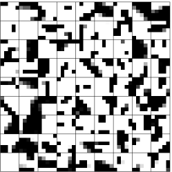
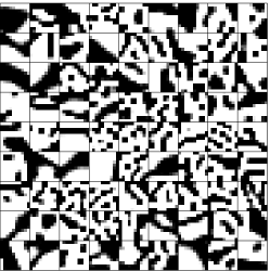
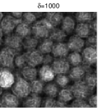
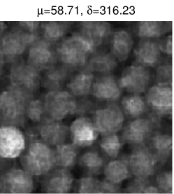
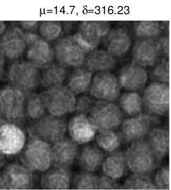
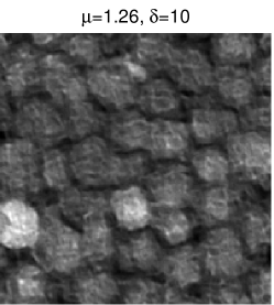
The set $\mathcal{D}_{\infty}$ corresponds to box constraints, and $\mathcal{D}_{2}$ is a spherical sector of the 2-norm ball with radius $\sqrt{p}$ . As we will see in the next section, the use of $\mathcal{D}_{\infty}$ as a prior gives rise to binary-looking images (corresponding to the vertices of $\mathcal{D}_{\infty}$ ) whereas $\mathcal{D}_{2}$ gives rise to more “natural looking” images.

We emphasize an important difference between the classical K-SVD method and our method. While K-SVD requires that we explicitly set the sparsity level, in our approach we affect sparsity implicitly through $1$ -norm regularization and via the regularization parameter $\lambda$ .

We use the Alternating Direction Method of Multipliers (ADMM) [Boyd] to compute an approximate local minimizer of (4). Learning the dictionary with the ADMM method has the advantages that the updates are cheap to compute, making the method suited for large-scale problems. The implementation details are described in the Appendix.

3.2 The Reconstruction Problem

Recall that we formulate the CT problem as $Ax\approx b$ , where $b$ contains the noisy data and $A$ is the system matrix. The vector $x$ represents an $M\times N$ image of absorption coefficients, and these coefficients must be nonnegative to have physical meaning. Hence we must impose a nonnegativity constraint on the solution.

Let us turn to the reconstruction problem based on the patch dictionary $D$ and the formulation (3). For ease of our presentation we assume that the image size $M\times N$ is a multiple of the patch size $P\times Q$ , and we partition the image into an $(M/P)\times(N/Q)$ array of non-overlapping blocks or patches represented by the vectors $x_{j}\in\mathbb{R}^{p}$ for $j=1,\ldots,q=(M/P)(N/Q)$ . The advantage of using non-overlapping blocks, compared to overlapping blocks, is that we avoid over-smoothing the image textures when averaging over the overlapping regions, and it requires less computing time.

Each block of $x$ is expressed as a conic combination of dictionary images, and hence the dictionary prior is expressed as

\Pi\,x=W\alpha,\quad W=(I\otimes D),\qquad\alpha\geq 0,

(5)

where $\Pi$ is a permutation matrix that re-orders the vector $x$ such that we reconstruct the image block by block, $W$ is the global dictionary, and

\alpha=\begin{pmatrix}\alpha_{1}\\ \vdots\\ \alpha_{q}\end{pmatrix}\in\underbrace{\mathbb{R}^{s}\times\cdots\times\mathbb{R}^{s}}_{\hbox{$q$ times}}

is a vector of coefficients for each of a total of $q$ blocks. With this non-overlapping formulation, it is straightforward to determine the numebr of unknowns in the problem (10). The length of $\alpha$ is $sq=n\,s/p$ which is equal to the product of the over-representation factor $s/p$ and the number of pixels $n$ in the image.

Figure 1: Polyhedral cone in

\mathbb{R}_{+}^{p}

spanned by five nonnegative dictionary elements, where

e_{i}

denotes the

i

th canonical unit vector in

\mathbb{R}^{s}

In pursuit of a nonnegative image $x$ , we impose the constraint that the vector $\alpha$ should be nonnegative. This implies that each block $x_{j}$ of $x$ lies inside a polyhedral cone

\displaystyle\mathcal{C}=\{Dz\,|\,z\in\mathbb{R}_{+}^{s}\}\subseteq\mathbb{R}_{+}^{p}

(6)

as illustrated in Figure 1. Clearly, if the dictionary contains the standard basis of $\mathbb{R}^{p}$ then $\mathcal{C}$ is equivalent to the entire nonnegative orthant in $\mathbb{R}^{p}$ . However, if the cone $\mathcal{C}$ is a proper subset of $\mathbb{R}_{+}^{p}$ , then not all nonnegative images have an exact representation in $\mathcal{C}$ , and hence the constraints $x_{j}\in\mathcal{C}$ may have a regularizing effect even without a sparsity prior on $\alpha$ . This can also be motivated by the fact that the faces of the cone $\mathcal{C}$ consist of images $x_{j}$ that can be represented as a conic combination of at most $p-1$ dictionary images.

Adding a sparsity prior on $\alpha$ , in addition to nonnegativity constraints, corresponds to the assumption that $x_{j}$ can be expressed as a conic combination of a small number of dictionary images and hence provides additional regularization. We include a 1-norm regularizer in our reconstruction problem as the standard approximate sparsity prior on $\alpha$ .

Reconstruction based on non-overlapping blocks often gives rise to block artifacts in the reconstruction because the objective in the reconstruction problem does not penalize jumps across the boundaries of neighboring blocks. To mitigate this type of artifact, we add a penalty term that discourages such jumps. We choose a penalty of the form

\psi(z)={\textstyle\frac{1}{2}}\,\|L\,z\|_{2}^{2}/\ell,\quad\ell=M(M/P-1)+N(N/Q-1)

(7)

where $L$ is a matrix such that $L\,z$ is a vector with finite-difference approximations of the directional derivatives across the block boundaries. The factor $\ell$ is the total number of pixels along the boundaries of the blocks in the image.

The constrained least squares reconstruction problem is then given by

\displaystyle\begin{array}[]{ll}\mbox{minimize}_{\alpha}&{\textstyle\frac{1}{2}}\frac{1}{m}\|A\Pi^{T}(I\otimes D)\alpha-b\|_{2}^{2}+\mu\,\frac{1}{q}\|\alpha\|_{1}+\delta^{2}\,\psi(\Pi^{T}(I\otimes D)\alpha)\\ \mbox{subject to}&\alpha\geq 0\end{array}

(10)

with regularization parameters $\mu,\delta>0$ . We normalize the problem formulation by i) division of the squared residual norm by the number of measurement $m$ , ii) division of the 1-norm of $\alpha$ by the number of blocks $q$ , and iii) division by $\ell$ in the function $\psi$ . Problem (10) is convex and it is an instance of a sparse approximation problem similar to formulations studied in [Elad].

4 Numerical Experiments

In this section we use numerical examples to demonstrate and quantify the behavior of our two-stage algorithm and evaluate the computed reconstructions. In particular we explore the influence of the dictionary structure and its parameters (number of elements, patch sizes) on the reconstruction, in order to illustrate the role of the learned dictionary.

The underlying idea is to compute a regularized least squares fit in which the solution is expressed in terms of the dictionary, and hence it lies in the cone $\mathcal{C}$ (6) defined by the dictionary elements. Hence there are two types of errors in the reconstruction process. Typically, the exact image does not lie in the cone ${\mathcal{C}}$ , leading to an approximation error. Moreover, we encounter a regularization error due to the combination of the error present in the data and the regularization scheme.

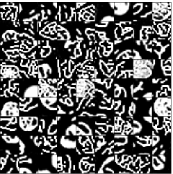
In the learning stage we use a set of images which are similar to the ones we wish to reconstruct. The ground-truth or exact image $x^{\mathrm{exact}}$ is not contained in the training set, so that we avoid committing an inverse crime. All images are gray-level and scaled in the interval $[0,1]$ .

All experiments were run in MATLAB (R2011b) on a 64-bit Linux system. The reconstruction problems are solved using the software package TFOCS (Templates for First-Order Conic Solvers) [Becker]. We compare with TV reconstructions computed by means of the MATLAB software TVReg [Jensen], with filtered back projection solutions computed by means of MATLAB’s “iradon” function, and solutions computed by means of the algebraic reconstruction technique (ART, also known as Kaczmarz’s method) with nonnegativety constraints implemented in the MATLAB package AIR Tools [HansenHansen]. (We did not compare with Krylov subspace methods because they are inferior to ART for images with sharp edges.)

4.1 The Test Image and the Tomographic Test Problem

The test images used in Sections 4.2–4.5 are square patches from a high-resolution photo of peppers with uneven surfaces resembling texture, making them interesting test images for studies of the reconstruction of textures and structures with sharp boundaries. Figure 2 shows the $1600\times 1200$ high-resolution image and the exact image of dimensions $M\times N=200\times 200$ . This size allows us to perform many numerical experiments in a reasonable amount of time; we demonstrate the performance of our algorithm on a larger test problem in Section 4.6.

Refer to caption — Figure 2: Left: the high-resolution image from which we obtain the training image patches. Right: the $200\times 200$ exact image $x^{\mathrm{exact}}$ .

All test problems represent a parallel-beam tomographic measurement, and we use the function paralleltomo from AIR Tools [HansenHansen] to compute the system matrix $A$ . The data associated with a set of parallel rays is called a projection, and number of rays in each projection is given by $N_{\mathrm{r}}=\lfloor\sqrt{2}N\rfloor$ . If the total number of projections is $N_{\mathrm{p}}$ then the number of rows in $A$ is $m=N_{\mathrm{r}}N_{\mathrm{p}}$ while the number of columns is $n=MN$ . Recall that we are interested in scenarios with a small number of projections. The exact data is generated with the forward model after which we add Gaussian white noise, i.e., $b=Ax^{\mathrm{exact}}+e$ .

4.2 Studies of the Dictionary Learning Stage

A good dictionary should preserve the structural information of the training images as much as possible and, at the same time, admit a sparse representation as well as a small representation error. These requirements are related to the number of dictionary elements, i.e., the number of columns $s$ in the matrix $D\in\mathbb{R}^{p\times s}$ . Since we want a compressed representation of the training images we choose $s$ such that $p\leq s\ll t$ , and the precise value will be investigated. The optimal patch size $P\times Q$ is unclear and will also be studied; without loss of generality we assume $P=Q$ .

The regularization parameter $\lambda$ in (4) balances the matrix factorization error and the sparsity constraint on the elements of the matrix $H$ . The larger the $\lambda$ , the more weight is given to minimization of $\|H\|_{\mathrm{sum}}$ , while for small $\lambda$ more weight is given to minimization of the factorization error. If $\lambda=0$ then (4) reduces to the classical nonnegative matrix factorization problem.

From the analysis of the upper bound on the regularization parameter $\lambda$ in the Appendix, we know $\lambda\geq p$ implies $H=0$ ; so $\lambda$ can be varied in the interval $(0,p]$ to find dictionaries with different sparsity priors. Note that the scaling of the training images affects the scaling of the matrix $H$ as well as the regularization parameter $\lambda$ .

To evaluate the impact of the dictionary parameters, we use three different patch sizes ( $5\times 5$ , $10\times 10$ , and $20\times 20$ ) and the number of dictionary elements $s$ is chosen to be 2, 3, and 4 times the of the number of rows $p$ in the dictionary $D$ . We extract more than $50,000$ overlapping patches from the high-resolution image in Figure 2. For different combinations of patch sizes and number of dictionary elements we solve the dictionary learning problem (4).

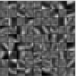
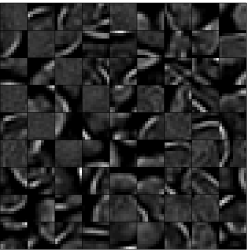
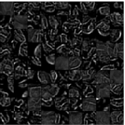
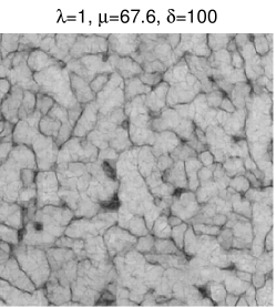
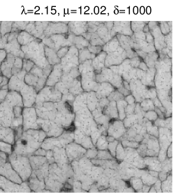
Figure 3 shows examples of such learned dictionaries, where columns of $D$ are represented as images; we see that the penalty constraint $D\in\mathcal{D}_{\infty}$ gives rise to “binary looking” dictionary elements while $D\in\mathcal{D}_{2}$ results in dictionary elements that use the whole gray-scale range.

To evaluate the approximation error, i.e., the distance of the exact image $x^{\mathrm{exact}}$ to its projection on the cone $\mathcal{C}$ (6), we compute the solutions $\alpha_{j}^{\star}$ to the $q$ approximation problems for all blocks $j=1,2,\ldots,q$ in $x^{\mathrm{exact}}$ ,

\min_{\alpha_{j}}{\textstyle\frac{1}{2}}\bigl{\|}D\alpha_{j}-x^{\mathrm{exact}}_{j}\bigr{\|}_{2}^{2}\qquad\mathrm{s.t.}\qquad\alpha_{j}\geq 0.

(11)

Then $P_{\mathcal{C}}(x_{j}^{\mathrm{exact}})=D\alpha_{j}^{\star}$ is the best representation/approximation of the $j$ th block in the cone. The mean approximation error (MAE) is then computed as

\mathrm{MAE}=\frac{1}{q}\sum_{j=1}^{q}\frac{1}{\sqrt{p}}\bigl{\|}P_{\mathcal{C}}(x_{j}^{\mathrm{exact}})-x_{j}^{\mathrm{exact}}\bigr{\|}_{2}.

(12)

[Uncaptioned image] — Figure 4: Mean approximation errors (12) for both $D\in\mathcal{D}_{\infty}$ and $D\in\mathcal{D}_{2}$ with different patch sizes and different $s$ .

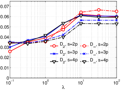
The ability of the dictionary to represent features and textures from the training images, which determines how good reconstructions we are able to compute, depends on the regularization parameter $\lambda$ , the patch size, and the number of dictionary elements. Figure 4 shows how the mean approximation error MAE (12) associated with the dictionary varies with patch size $p$ , number of dictionary elements $s$ , and regularization parameter $\lambda$ . An advantage of larger patch sizes is that the variation of MAE with $s$ and $\lambda$ is less pronounced than for small patch sizes, so overall we tend to prefer larger patch sizes. In particular, for a large patch size we can use a smaller over-representation factor $s/p$ than for a small patch size. As $\lambda$ approaches $p$ we have that $\|H\|_{\mathrm{sum}}$ approaches 0, the dictionary $D$ takes arbitrary values, and the approximation errors level off at a maximum value. Regarding the two different constraints $D\in\mathcal{D}_{\infty}$ and $D\in\mathcal{D}_{2}$ we do not see any big difference in the approximation errors for $10\times 10$ and $20\times 20$ patches; to limit the amount of results we now use $\mathcal{D}_{2}$ .

The computational work depends on the patch size and the number of dictionary elements which, in turn, affects the approximation error: the larger the dictionary, the smaller the approximation error, but at a higher computational cost. We have found that a good trade-off between the computational work and the approximation error can be obtained by increasing the number of dictionary elements until the approximation error levels off.

4.3 Studies of the Reconstruction Stage

Here we evaluate the overall reconstruction framework including the effect of the reconstruction parameters as well as their connection to the dictionary learning parameter $\lambda$ and the patch size.

We solve the reconstruction problem (10) using projection data based on the exact image given in Figure 2. We choose $N_{\mathrm{p}}=25$ uniformly distributed projection angles in $[0^{\circ},180^{\circ}]$ . Hence the matrix $A$ has dimensions $m=7,050$ and $n=40,000$ , so the problem is highly underdetermined. We use the relative noise level $\|e\|_{2}/\|Ax^{\mathrm{exact}}\|_{2}=0.01$ . Moreover, we use $5\times 5$ , $10\times 10$ and $20\times 20$ patches and corresponding dictionary matrices $D^{(5)}$ , $D^{(10)}$ , and $D^{(20)}$ in $\mathcal{D}_{2}$ of size $25\times 100$ , $100\times 300$ , and $400\times 800$ , respectively. Examples of the dictionary elements are shown in the bottom row of Figure 3.

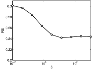
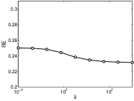
We first investigate the reconstruction’s sensitivity to the choice of $\lambda$ in the dictionary learning problem and the parameters $\mu$ and $\delta$ in the reconstruction problem. It follows from the optimality conditions of (10) that $\alpha^{\star}=0$ is optimal when $\mu\geq\bar{\mu}=\frac{q}{m}\|(I\otimes D^{T})\Pi A^{T}b\|_{\infty}$ and hence we choose $\mu\in[0,\bar{\mu}]$ . Large values of $\mu$ refer to the case where the sparsity prior is strong and the solution is presented with too few dictionary elements. On the other hand if $\mu$ is small and a sufficient number of dictionary elements are included, the reconstruction error worsens only slightly when $\mu$ decreases. In the next subsection we show that we may, indeed, obtain reasonable reconstructions for $\mu=0$ .

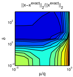
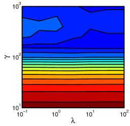
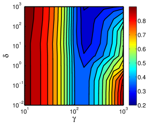
To investigate the effect of regularization parameters $\lambda$ and $\mu$ , we first perform experiments with $\delta=0$ corresponding to no image prior. The quality of a solution $x$ is evaluated by the reconstruction error

\mathrm{RE}=\|x-x^{\mathrm{exact}}\|_{2}/\|x^{\mathrm{exact}}\|_{2}

(13)

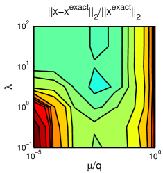
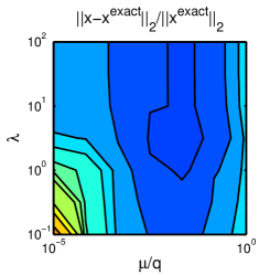
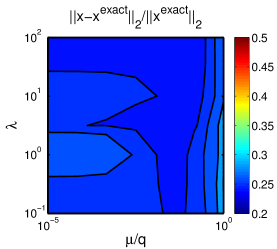
and Figure 5 shows contour plots of RE as a function of $\lambda$ and $\mu/q$ . The reconstruction error is smaller for larger patch sizes, and also less dependent on the regularization parameter $\lambda$ and the normalized regularization parameter $\mu/q$ . The smallest reconstruction errors are obtained in all dictionary sizes for $\lambda\approx 3$ .

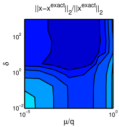
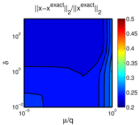
Let us now consider the reconstructions when $\delta>0$ in order to reduce block artifacts. Figure 6 shows contour plots of the reconstruction error versus $\mu/q$ and $\delta$ , using a fixed $\lambda=3.16$ . It is no surprise that introducing $\delta$ acts as a regularizer that can significantly reduce blocking artifacts and thus improve the reconstruction. Sufficiently large values of $\delta$ yield smaller reconstruction errors. Consistent with the results from Figure 5, the reconstruction errors are smaller for $10\times 10$ and $20\times 20$ patch sizes than for $5\times 5$ patches. For larger patch sizes (which allow for capturing more structure in the dictionary elements) the reconstruction error is quite insensitive to the choice of $\delta$ and $\mu$ . The contour plots in Figure 6 suggest that with our problem specification, we should choose $\delta\geq 1$ .

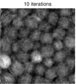
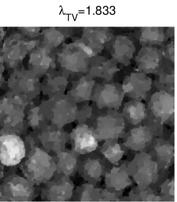
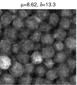
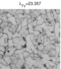
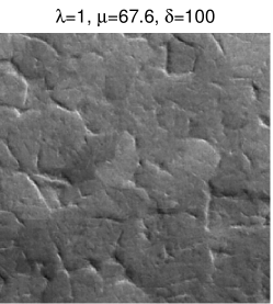
Finally, in Figure 7 we compare our reconstructions with those computed by means of filtered back projection (FBP), the algebraic reconstruction technique (ART), and TV regularization. We used the Shepp-Logan filter in “iradon.” To be fair, the TV regularization parameter and the number of ART iterations were chosen to yield an optimal reconstruction.

•

The FBP reconstruction contains the typical artifacts associated with this method for underdetermined problems, such as line structures.
•

The ART reconstruction – although having about the same RE as our reconstruction – is blurry and contains artifacts such as circle structures and errors in the corners.
•

The TV reconstruction has the typical “cartoonish” appearance of TV solutions and hence it fails to include most of the details associated with the texture; the edges of the pepper grains are distinct but geometrically somewhat un-smooth.
•

Our reconstructions, while having about the same RE as the TV reconstruction, include more texture and some of the details from the exact image (but not all) are recovered, especially with $D^{(20)}$ . Also the pepper grain edges resemble more the smooth edges from the exact image.

We conclude that our dictionary-based reconstruction method appears to have an edge over the other three methods.

Our formulation in (10) enforces that the solution is an exact representation in the dictionary, and searching for solutions in the cone spanned by the dictionary elements is a strong assumption in the reconstruction formulation. In [Soltani] we investigated this requirement experimentally and showed that relaxing the equality $\Pi x=(I\otimes D)$ does not give an advantage, i.e., approximating a solution by $\Pi x\approx(I\otimes D)\alpha$ and minimizing $\|\Pi x-(I\otimes D)\alpha\|_{2}$ does not improve the reconstruction quality, and one can compute a good reconstruction as a conic combination of the dictionary elements.

4.4 Simplifying the Computational Problem

We have been working under the assumption that $\alpha\geq 0$ and that it is sparse. Imposing both non-negativity and a 1-norm constraint on the representation vector $\alpha$ are strong assumptions in the reconstruction formulation. If we drop the non-negativity constraint in the image reconstruction problem, then (10) takes the form of a constrained least squares problem:

\min_{\alpha}\frac{1}{2}\left\|\begin{pmatrix}\frac{1}{\sqrt{m}}A\,\Pi^{\mathrm{T}}(I\otimes D)\\[5.69054pt] \frac{\delta}{\sqrt{\ell}}L\,\Pi^{\mathrm{T}}(I\otimes D)\end{pmatrix}\alpha-\begin{pmatrix}b\\ 0\end{pmatrix}\right\|_{2}^{2}\qquad\text{s.t.}\quad\|\alpha\|_{1}\leq\gamma,

(14)

where $\gamma>0$ . Alternatively we can neglect the parameter $\mu$ . This is motivated by the plots in Figures 5 and 6 which suggest that for sufficiently large $\lambda$ , $\delta$ and patch sizes, the reconstruction error is almost independent of $\mu$ as long as it is small. When $\mu=0$ (10) reduces to a nonnegatively constrained least square problem:

\min_{\alpha}\frac{1}{2}\left\|\begin{pmatrix}\frac{1}{\sqrt{m}}A\,\Pi^{\mathrm{T}}(I\otimes D)\\[5.69054pt] \frac{\delta}{\sqrt{\ell}}L\,\Pi^{\mathrm{T}}(I\otimes D)\end{pmatrix}\alpha-\begin{pmatrix}b\\ 0\end{pmatrix}\right\|_{2}^{2}\qquad\text{s.t.}\qquad\alpha\geq 0.

(15)

We use the same test problem with $25$ projections and relative noise level 0.01 as in Section 4.3. We solve problem (14) for $D^{(10)}\in\mathcal{D}_{2}$ , which resulted in the smallest reconstruction error when solving (10) (cf. Figure 7). Likewise we choose $10\times 10$ and $20\times 20$ patch sizes and $D^{(10)},D^{(20)}\in\mathcal{D}_{2}$ to solve (15). Figures 8 and 9 show the respective reconstructions.

There are two difficulties with the reconstructions computed via (14). The lack of a nonnegativity constraint on $\alpha$ can lead to negative pixel values in the reconstruction, and this is undesired because it is nonphysical and it leads to a larger reconstruction error . Also, as can be seen in Figure 8, the reconstruction is very sensitive to the choose of the regularization parameter $\gamma$ ; it must be sufficiently large to allow the solution to be represented with a sufficient number of dictionary elements, and it should be carefully chosen to provide an acceptable reconstruction.

The solution to problem (15) for a $20\times 20$ patch size, compared to the solution shown in Figure 7, is not significantly worse both visually and in terms of reconstruction error. This suggests that using the dictionary obtained from (4) with a proper choice of $\lambda$ and patch size and a nonnegatively constraint may be sufficient for the reconstruction problem, i.e., we can let $\mu=0$ . While this seems to simplify the problem – going from (10) to (15) – it does not significantly simplify the computational optimization problem, since the 1-norm constraint is handled by simple thresholding in the software; but it help us to get rid of a parameter in the reconstruction process. However, when the 1-norm constraint is omitted, additional care is necessary when choosing $\lambda$ and the patch sizes to avoid introducing artifacts or noise.

4.5 Studies of Robustness

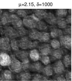
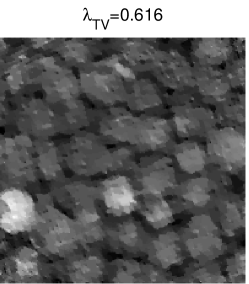
To further study the performance of our algorithm, in this section we consider reconstructions based on (10) with more noise in the data, and with projections within a limited range. The first two tests use $25$ and $50$ projections with uniform angular sampling in $[0^{\circ},180^{\circ}]$ and with relative noise level = 0.05, i.e., a higher noise level than above. For our highly underdetermined problems we know that both filtered back projection and algebraic iterative techniques give unsatisfactory solutions, and therefore we only compare our method with TV. As before the regularization parameters $\lambda$ and $\mu$ are chosen from numerical experiments such that a solution with the smallest error is obtained.

The reconstructions are shown in the top and middle rows of Figure 10. The reconstruction errors are still similar across the methods. Again, the TV reconstructions have the characteristic “cartoonish” appearance while the dictionary-based reconstructions retain more the structure and texture but have other artifacts – especially for $N_{\mathrm{p}}=25$ . We also note that these artifacts are different for the two different dictionaries.

The third set uses $25$ projections uniformly distributed in the limited range $[0^{\circ},120^{\circ}]$ and with relative noise level 0.01. In this case the TV reconstructions display additional artifacts related to the limited-angle situation, while such artifacts are somewhat less pronounced in the reconstructions by our algorithm.

In the numerical studies performed in this paper there is an underlying assumption that the scale and orientation of the training images are consistent with the unknown image. While this assumption is convenient for the studies performed here, it may not be entirely realistic. In a separate work [Soltani] we therefore investigated the sensitivity and robustness of the reconstruction to variations of the scale and orientation in the training images, and we discuss algorithms to estimate the correct relative scale and orientation from the data (scale being the more difficult parameter to estimate).

4.6 A Large Test Case

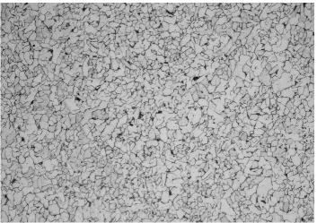
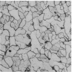
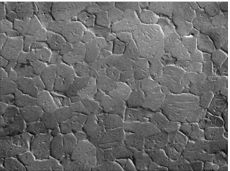
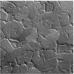
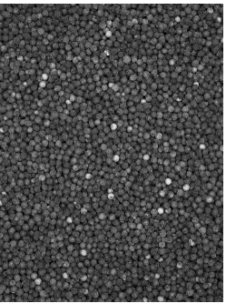
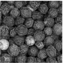
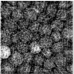
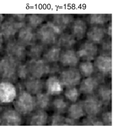
We finish the numerical experiments with a verification of our method on two larger test problems that simulate the analysis of microstructure in materials science. Almost all common metals and many ceramics are polycrystalline, i.e., they are composed of many small crystals or grains of varying size and orientation, and the variations in orientation can be random. It is of particular interest to study how the grain boundaries — the interfaces between grains — respond external stimuli such heat, stress or strain. Here we assume that priors of the grain structure are available in the form of training images.

The simulated data was computed using images of steel and zirconium grains. The steel microstructure image from [steel] is of dimensions $900\times 1280$ and the zirconium grain image (produced by a scanning electron microscope) is $760\times 1020$ . More than $50,000$ patches are extracted from these images to learn dictionaries $D^{(20)}\in\mathcal{D}_{2},\mathcal{D}_{\infty}$ of size $400\times 800$ . To avoid doing inverse crime, we obtain the exact images of dimensions $520\times 520$ by first rotating the high-resolution image and then extracting the exact image. The high-resolution images and the exact images are shown in Figure 11.