Ultrafast spin dynamics in II-VI diluted magnetic semiconductors with spin-orbit interaction

Abstract

We study theoretically the ultrafast spin dynamics of II-VI diluted magnetic semiconductors in the presence of spin-orbit interaction. Our goal is to explore the interplay or competition between the exchange $sd$-coupling and the spin-orbit interaction in both bulk and quantum well systems. For bulk materials we concentrate on Zn_1-xMn_xSe and take into account the Dresselhaus interaction, while for quantum wells we examine Hg_1-x-yMn_xCd_yTe systems with a strong Rashba coupling. Our calculations were performed with a recently developed formalism which incorporates electronic correlations beyond mean-field theory originated from the exchange $sd$-coupling. For both bulk and quasi-two-dimensional systems we find that, by varying the system parameters within realistic ranges, both interactions can be chosen to play a dominant role or to compete on an equal footing with each other. The most notable effect of the spin-orbit interaction in both types of systems is the appearance of strong oscillations where the exchange $sd$-coupling by itself only causes an exponential decay of the mean electronic spin components. The mean-field approximation is also studied and it is interpreted analytically why it shows a strong suppression of the spin-orbit-induced dephasing of the spin component parallel to the Mn magnetic field.

I Introduction

Diluted magnetic semiconductors (DMS) are multifunctional materials that combine the outstanding electronic and optical properties of semiconductors with highly controllable magnetic properties. kos-gaj ; xia-ge-cha With the prospect of spintronic applications of DMS in mind, much effort has focused recently on the study of ultrafast spin dynamics and control. kir-kim-ras ; qi-xu-ste ; has-kob-mun ; cyw-sha ; mor-her-man ; kap-per-wic ; thu-axt-win At the same time, spin-orbit interaction (SOI) effects have been intensely studied in non-magnetic bulk and nanostructured semiconductors. win ; zut-fab-das ; fab-etal ; dya ; wu-jia-wen ; tsy-zut The interplay between the exchange interaction characteristic of DMS and the more generic SOI can lead to new possibilities for applications and basic research. gna-nav ; yan-cha-wu ; val-mir ; jia-zho-kor ; mir-sho-ela ; den-ave In particular, the spin-orbit torque effect in DMS has attracted much interest in recent years. man-zha ; gar-mac ; hal-bra-tse ; che-ove-liu ; end-mat-ohn ; fan-kur-wun ; li-wan-doa ; lin-wan-per

In this article we explore theoretically this interplay by studying the ultrafast spin dynamics of a non-equilibrium electron distribution in the conduction band of II-VI Mn-doped semiconductors. Our work is based on a microscopic density-matrix theory that models on a quantum-kinetic level the spin precession and the spin transfer between electrons in the conduction band of such semiconductors and the manganese electrons, and which accounts for exchange-induced correlations beyond the mean-field level and considers the localized character of the Mn spins.thu-axt This recently developed formalism is quite general and can be computationally costly to apply in some circumstances. For this reason, in the present study we consider a particular situation which is nevertheless experimentally relevant and theoretically interesting: the limit of high Mn density compared to the electron density, which is normally realized in photoexcitation experiments. In this particular regime we can apply a simplified formalism which captures the essential physics that is relevant here and which reduces greatly the numerical effort.cyg-axt-15

The purpose of our study is to determine under which conditions, if any, the spin-orbit interaction mechanisms present in semiconductors can become relevant or even dominant in the picosecond time-scale spin dynamics in DMS. As will be seen here, for both bulk and quasi-two-dimensional systems, depending on the choice of material parameters and excitation conditions, there can be a strong interplay or competition between the two types of interactions. This rather unexplored combined effect between exchange and SOI in DMS could lead in principle to new forms of spin control suitable for spintronic applications.

This article is organized as follows. In Section II.1 we present the model Hamiltonian of the DMS with spin-orbit interaction and in Section II.2 we review the equations of motion that describe the spin dynamics in the formalism adopted here. In Sections III and IV we present and discuss our results for bulk Zn_1-xMn_xSe and for Hg_1-x-yMn_xCd_yTe quantum wells, respectively. Finally, we provide some concluding remarks.

II Quantum kinetic formalism

II.1 DMS Hamiltonian

The theoretical model of DMS for our work includes the exchange $sd$-coupling between electrons in the conduction band and $d$-electrons of the doping Mn atoms and the SOI of conduction-band electrons expressed in the envelope-function approximation. The Hamiltonian has the form

$$H=H_{0}+H_{sd}+H_{\text{SO}}\,,$$ (1)

where $H_{0}=\sum_{i}\mathbf{p}_{i}^{2}/2m^{\ast}$, with conduction-band effective mass $m^{\ast}$, and the Kondo-like Hamiltonian thu-axt

$$H_{sd}=J_{sd}\sum_{iI}\mathbf{s}_{i}\cdot\mathbf{S}_{I}\,\delta(\mathbf{r}_{i}-\mathbf{R}_{I})$$ (2)

describes the coupling due to the exchange interaction between the conduction-band electrons and the Mn electrons. The spin operator and position of the $I$-th Mn atom ($i$-th conduction-band electron) are denoted as $\mathbf{S}_{I}$ and $\mathbf{R}_{I}$ ($\mathbf{s}_{i}$ and $\mathbf{r}_{i}$), respectively. The coupling constant $J_{sd}$ is negative here, corresponding to a ferromagnetic coupling.cib-sca In the present work the negative Landé-factor of Mn will always be combined with the negative sign of the coupling constant $J_{sd}$. In addition, all spin variables will be considered dimensionless and the coupling constant accordingly modified.

For bulk materials, the SOI Hamiltonian $H_{\text{SO}}$ of zincblende semiconductors is the Dresselhaus Hamiltonian dre

$$H_{\text{D}}=\gamma_{\text{D}}\sum_{i}[\sigma_{i,x}k_{i,x}(k_{i,y}^{2}-k_{i,z}^{2})+\text{cyclic perm.}]\,,$$ (3)

where $\boldsymbol{\sigma}$ is the vector of Pauli matrices and $\mathbf{k}$ is the operator $\mathbf{p}/\hbar$. For quasi-two-dimensional systems, we consider asymmetric quantum wells which display the Rashba SOI ras

$$H_{R}=\alpha_{\text{R}}\sum_{i}(k_{i,y}\sigma_{i,x}-k_{i,x}\sigma_{i,y})\,.$$ (4)

These effective spin-orbit couplings can be thought of as interactions of a spin with $\mathbf{k}$-dependent magnetic fields.

II.2 Equations of motion

In Refs. [thu-axt, ], [cyg-axt-15, ], and [cyg-axt, ], the Heisenberg equations of motion of the density matrix for DMS without SOI were posed and analyzed in terms of a correlation hierarchy which includes averaging of the Mn-atom positions, thus rendering the problem spatially homogeneous. In this work we follow that formalism and extend it in a simple fashion in order to study the effects of the SOI on the electronic spin degree of freedom.

When the number of Mn atoms ($N_{\text{Mn}}$) is much larger than the number of conduction-band electrons ($N_{\text{e}}$), i.e. in the limit $N_{\text{Mn}}\gg N_{\text{e}}$, the quantum kinetic equations established in Ref. [thu-axt, ] can be significantly simplified. This assumption can be easily fulfilled for intrinsic semiconductors in which the Mn²⁺ ions are incorporated isoelectronically, like in the case of II-VI semiconductors.fur-kos Unlike the situation in, for example, III-V based DMS, where the Mn doping results in a large number of holes, in isoelectronically doped systems the density of free carriers is controlled solely by the photoexcitation and thus can be kept much smaller than the Mn density simply by using low laser intensities. Here we consider electrons excited with typical narrow-band laser pulses with near-bandgap energies and low intensities. Employing the approximation of low-electron density as compared to the Mn doping density, we have developed a simplified formalism cyg-axt-15 based on the full model of Ref. [thu-axt, ] which allows a numerically efficient handling of electronic correlations. Here we adopt the low electron-density limit and follow the formalism of Ref. [cyg-axt-15, ].

In the regime $N_{\text{Mn}}\gg N_{\text{e}}$ the Mn density matrix can be considered stationary and we take the $z$-axis along the mean Mn magnetization $\langle\mathbf{S}\rangle$. The assumption of a stationary Mn density matrix has been numerically tested under conditions comparable with our present case in Refs. [cyg-axt-15, ], [cyg-axt, ], [thu-cyg-axt-kuh-b, ], and [thu-cyg-axt-kuh-a, ]. We introduce a precession frequency for the conduction-band electrons in the effective magnetic field of the Mn atoms

$$\omega_{\text{\tiny M}}=\frac{J_{sd}}{\hbar}n_{\text{Mn}}S\,,$$ (5)

where $n_{\text{Mn}}$ is the Mn density and $S=|\langle\mathbf{S}\rangle|$, with $0\leq S\leq\frac{5}{2}$.

We study the time evolution of the mean value of the spin operator associated with the state with wave vector $\mathbf{k}$,

$$\langle\mathbf{s}_{\mathbf{k}}\rangle=\sum_{\sigma\sigma^{\prime}}\mathbf{s}_{\sigma\sigma^{\prime}}\langle c_{\sigma\mathbf{k}}^{\dagger}c_{\sigma^{\prime}\mathbf{k}}\rangle=(\langle\mathbf{s}_{\mathbf{k}}^{\perp}\rangle,\langle s_{\mathbf{k}}^{\parallel}\rangle),$$ (6)

where $\langle\mathbf{s}_{\mathbf{k}}^{\perp}\rangle$ and $\langle s_{\mathbf{k}}^{\parallel}\rangle$ are the mean spin components perpendicular and parallel to the mean Mn magnetization, respectively [see Fig. 1(b)]. We will take as system variables $\langle\mathbf{s}_{\mathbf{k}}^{\perp}\rangle$ and the populations $n_{\mathbf{k}}^{\sigma}=\langle c_{\sigma\mathbf{k}}^{\dagger}c_{\sigma\mathbf{k}}\rangle$. The parallel mean spin can be obtained from the latter as

$$\langle s_{\mathbf{k}}^{\parallel}\rangle=\frac{1}{2}\left(n_{\mathbf{k}}^{\uparrow}-n_{\mathbf{k}}^{\downarrow}\right).$$ (7)

Leaving aside for the moment the SOI, the time evolution of these variables induced by $H_{0}$ and the $sd$-interaction is given by cyg-axt-15

$$\left.\frac{\partial}{\partial t}n_{\mathbf{k}}^{\uparrow/\downarrow}\right|_{\text{sd}}=\sum_{\mathbf{k^{\prime}}}\left[\Re(G_{\omega_{\mathbf{k^{\prime}}}}^{\omega_{\mathbf{k}}})\frac{b^{\parallel}}{2}\left(n_{\mathbf{k^{\prime}}}^{\uparrow/\downarrow}-n_{\mathbf{k}}^{\uparrow/\downarrow}\right)+\Re(G_{\omega_{\mathbf{k^{\prime}}}}^{\omega_{\mathbf{k}}\pm\omega_{\text{\tiny M}}})\left(b^{\pm}n_{\mathbf{k^{\prime}}}^{\downarrow/\uparrow}-b^{\mp}n_{\mathbf{k}}^{\uparrow/\downarrow}\mp 2b^{0}n_{\mathbf{k}}^{\uparrow/\downarrow}n_{\mathbf{k^{\prime}}}^{\downarrow/\uparrow}\right)\right]\,,$$ (8)

$$\left.\frac{\partial}{\partial t}\langle\mathbf{s}_{\mathbf{k}}^{\perp}\rangle\right|_{\text{sd}} = -\sum_{\mathbf{k^{\prime}}}\left\{\left[\Re(G_{\omega_{\mathbf{k^{\prime}}}}^{\omega_{\mathbf{k}}-\omega_{\text{\tiny M}}})\left(\frac{b^{+}}{2}\!-\!b^{0}n_{\mathbf{k^{\prime}}}^{\uparrow}\right)+\Re(G_{\omega_{\mathbf{k^{\prime}}}}^{\omega_{\mathbf{k}}+\omega_{\text{\tiny M}}})\left(\frac{b^{-}}{2}\!+\!b^{0}n_{\mathbf{k^{\prime}}}^{\downarrow}\right)\right]\langle\mathbf{s}_{\mathbf{k}}^{\perp}\rangle+\Re(G_{\omega_{\mathbf{k^{\prime}}}}^{\omega_{\mathbf{k}}})\frac{b^{\parallel}}{2}(\langle\mathbf{s}_{\mathbf{k^{\prime}}}^{\perp}\rangle+\langle\mathbf{s}_{\mathbf{k}}^{\perp}\rangle)\right\}$$ (9)

$$+ \left\{\omega_{\text{\tiny M}}-\sum_{\mathbf{k^{\prime}}}\left[\Im(G_{\omega_{\mathbf{k^{\prime}}}}^{\omega_{\mathbf{k}}-\omega_{\text{\tiny M}}})\left(\frac{b^{+}}{2}-b^{0}n_{\mathbf{k^{\prime}}}^{\uparrow}\right)-\Im(G_{\omega_{\mathbf{k^{\prime}}}}^{\omega_{\mathbf{k}}+\omega_{\text{\tiny M}}})\left(\frac{b^{-}}{2}+b^{0}n_{\mathbf{k^{\prime}}}^{\downarrow}\right)\right]\right\}\frac{\langle\mathbf{S}\rangle}{S}\times\langle\mathbf{s}_{\mathbf{k}}^{\perp}\rangle\,.$$

The constants in Eqs. (8) and (9) depend only on the setting of the Mn magnetization and are given by $b^{\pm}=\langle{S^{\perp}}^{2}\rangle\pm b^{0}$, $b^{0}=\langle S^{\parallel}\rangle/2$, $b^{\parallel}=\langle{S^{\parallel}}^{2}\rangle$, where $S^{\parallel}=\mathbf{S}\cdot\langle\mathbf{S}\rangle/S$, and $\langle{S^{\perp}}^{2}\rangle=\langle S^{2}-{S^{\parallel}}^{2}\rangle/2$. We also called $\omega_{\mathbf{k}}=E_{\mathbf{k}}/\hbar=\hbar\mathbf{k}^{2}/2m^{\ast}$.

The function $G_{\omega_{\mathbf{k^{\prime}}}}^{\omega_{\mathbf{k}}}$ can be interpreted as a memory function and has the form

$$G_{\omega_{\mathbf{k^{\prime}}}}^{\omega_{\mathbf{k}}}(t) = \frac{J_{sd}^{2}\,n_{\text{\tiny Mn}}}{V\hbar^{2}}\int_{-t}^{0}dt^{\prime}e^{i(\omega_{\mathbf{k^{\prime}}}-\omega_{\mathbf{k}})t^{\prime}}$$ (10)

$$\approx \frac{J_{sd}^{2}\,n_{\text{\tiny Mn}}}{V\hbar^{2}}\pi\delta(\omega_{\mathbf{k^{\prime}}}-\omega_{\mathbf{k}}),$$

where in the last step we neglected the imaginary part and the finite memory, i.e. we applied a Markov limit which is a good approximation for not too large values of $J_{sd}^{2}$ and excitations not too close to the band edge.thu-cyg-axt-kuh-a

The spin-orbit Hamiltonians of Eqs. (3) or (4) introduce, to a first approximation, an additional $\mathbf{k}$-dependent spin precession. If the contribution of a single electron with wave vector $\mathbf{k}$ to the spin-orbit Hamiltonian is written in the form

$$H_{\text{SO}}=\frac{\hbar}{2}\,\mathbf{\hat{\Omega}}_{\mathbf{k}}\cdot\boldsymbol{\sigma},$$ (11)

then the mentioned spin precession is described by the Heisenberg equation of motion of the mean value of the spin operator introduced in Eq. (6),

$$\left.\frac{\partial}{\partial t}\langle\mathbf{s}_{\mathbf{k}}\rangle\right|_{\text{SO}}=\mathbf{\Omega}_{\mathbf{k}}\times\langle\mathbf{s}_{\mathbf{k}}\rangle.$$ (12)

Note that while $\mathbf{\hat{\Omega}}_{\mathbf{k}}$ is an operator, we introduced $\mathbf{\Omega}_{\mathbf{k}}$ as the corresponding regular vector where $\mathbf{k}$ is interpreted simply as a wave vector and not as an operator as in Eqs. (3) and (4) [see Fig. 1(b)]. In the present study we take into account the influence of the spin-orbit interaction at this level, in order to elucidate how this added $\mathbf{k}$-dependent precession alters the quantum spin dynamics in bulk and quasi-two-dimensional DMS.

III Bulk Zn_1-xMn_xSe

In this Section we present ultrafast spin dynamics results for bulk semiconductors. For concreteness we focus on Zn_1-xMn_xSe which is currently one of the best studied II-VI DMS, and as we will see, it can display an interesting interplay between exchange and SOI. We first examine numerically and analytically the dephasing caused by the Dresselhaus spin-orbit coupling and then we proceed to calculate and analyze the full dynamics under the influence of both exchange coupling and SOI.

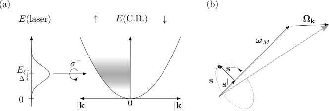
Figure 1: (a) Schematic representation of the conduction band (C.B.) and the spectrum of the circularly-polarized Gaussian laser pulse that excites electrons from the valence band to a Gaussian distribution of spin up electrons in the conduction band (centered at an energy $E_{C}$ above the band edge and with standard deviation $\Delta$). (b) The electron spin and its components $\langle\mathbf{s}_{\mathbf{k}}^{\perp}\rangle$ and $\langle s_{\mathbf{k}}^{\parallel}\rangle$, perpendicular and parallel to the Mn magnetic field (or equivalently angular frequency $\boldsymbol{\omega}_{\text{M}}$), respectively. Also represented is $\boldsymbol{\Omega}_{\mathbf{k}}$, the angular frequency associated with the $\mathbf{k}$-dependent spin-orbit effective magnetic field. The electron spin precesses about $\boldsymbol{\omega}_{\text{M}}+\boldsymbol{\Omega}_{\mathbf{k}}$.

III.1 Dresselhaus-induced dephasing

As mentioned in Sec. II.1, the spin-orbit interaction in the envelope-function approximation plays the role of an effective $\mathbf{k}$-dependent magnetic field around which the electron spin precesses. This spin precession in the case of an electron gas leads to global spin dephasing and decay, which is at the root of the D’yakonov-Perel spin-relaxation mechanism.dya-per As initial condition for the conduction-band electrons we assume a Gaussian distribution caused by a pulsed optical excitation, similar to the one illustrated in Fig. 1(a). For the moment we consider a Gaussian distribution centered at $E_{C}=0$ (the band edge) and later we will consider an excitation centered at $E_{C}=$10 meV, always with standard deviation $\Delta=$3 meV. We assume that the optical excitation populates only the spin-up conduction-band states thanks to its appropriate circular polarization. In Fig. 2 we plot the spin polarization, $\langle s_{z}\rangle(t)=2N_{\text{e}}^{-1}\sum_{\mathbf{k}}\langle s_{\mathbf{k},z}\rangle(t)$ (normalized to 1), of the initially spin-up electron population (the $z$-axis coincides with the main axis of the zincblende lattice) in the conduction band versus time for different values of the Dresselhaus spin-orbit coupling constant $\gamma_{D}$.

The accepted standard value of $\gamma_{\text{D}}/\hbar=13.3\,\text{ps}^{-1}\text{nm}^{3}$ is included,win and two artificially high values (40 and 100 $\text{ps}^{-1}\text{nm}^{3}$) are added to explore the tendencies of the decay behavior. We use for the conduction-band effective mass of ZnSe the value $m^{\ast}=0.134\,m_{0}$,yu-car where $m_{0}$ is the bare electron mass. The expected dephasing and decay mentioned above is clearly observed, with faster decay obtained for increasing SOI coupling constant. Note that the decay, however, is not exponential from the beginning, but rather quadratic at short times. Another interesting feature is that for an excitation 10 meV above the band edge the evolution displays a non-monotonic behavior. Below we shall indicate the origin of this incipiently oscillatory behavior.

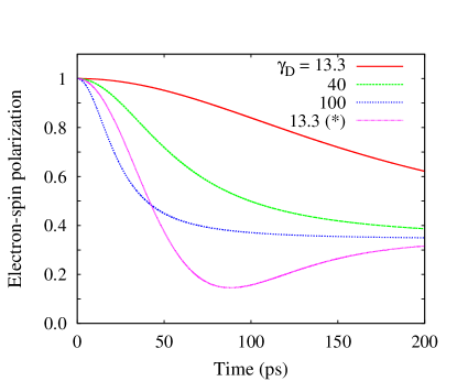
Figure 2: Dephasing after isotropic Gaussian excitation of the spin-up band (standard deviation $\Delta=$3 meV) without exchange $sd$-coupling in an effective Dresselhaus spin-orbit magnetic field with prefactor $\gamma_{D}$, specified in $\mbox{ps}^{-1}\mbox{nm}^{3}$. Three of the curves correspond to a Gaussian excitation centered at the band edge ($E_{C}=0$), while the fourth, marked with (*), corresponds to a displacement of the excitation to $E_{C}=$10 meV above the band edge.

The long-time limit of the spin polarization seen in Fig. 2, which corresponds to the equilibrium distribution caused by the SOI effective field dephasing, is given by the value 1/3:

$$\lim_{t\rightarrow\infty}\langle s_{z}\rangle(t)=:\langle s_{eq}\rangle=\frac{1}{3}\langle s_{z}\rangle(t=0).$$ (13)

This equilibrium value can be understood analytically as follows. The equation of motion for the spin under the SOI effective magnetic field, $\left.\frac{\partial}{\partial t}\langle\mathbf{s}_{\mathbf{k}}\rangle\right|_{\text{SO}}={\mathbf{\Omega}_{\mathbf{k}}}\times\langle\mathbf{s}_{\mathbf{k}}\rangle$, can be cast in the matrix form $\left.\frac{\partial}{\partial t}\langle\mathbf{s}_{\mathbf{k}}\rangle\right|_{\text{SO}}=\mathbb{M}_{\mathbf{k}}\langle\mathbf{s}_{\mathbf{k}}\rangle$, where

$$\mathbb{M}_{\mathbf{k}}=\left(\begin{array}[]{ccc}0&-\Omega_{\mathbf{k},z}&\Omega_{\mathbf{k},y}\\ \Omega_{\mathbf{k},z}&0&-\Omega_{\mathbf{k},x}\\ -\Omega_{\mathbf{k},y}&\Omega_{\mathbf{k},x}&0\\ \end{array}\right),$$ (14)

and has the formal solution

$$\langle\mathbf{s}_{\mathbf{k}}\rangle(t)=\exp(\mathbb{M}_{\mathbf{k}}t)\,\langle\mathbf{s}_{\mathbf{k}}\rangle(0).$$ (15)

The Taylor expansion of the matrix exponential can be simplified using that $\mathbb{M}_{\mathbf{k}}^{3}=-\Omega_{\mathbf{k}}^{2}\,\mathbb{M}_{\mathbf{k}}$ and $\mathbb{M}_{\mathbf{k}}^{4}=-\Omega_{\mathbf{k}}^{2}\,\mathbb{M}_{\mathbf{k}}^{2}$, with $\Omega_{\mathbf{k}}=|\boldsymbol{\Omega}_{\mathbf{k}}|$. One obtains

$$\exp(\mathbb{M}_{\mathbf{k}}t)=1+\sin(\Omega_{\mathbf{k}}t)\,\frac{\mathbb{M}_{\mathbf{k}}}{\Omega_{\mathbf{k}}}+\left[1-\cos(\Omega_{\mathbf{k}}t)\right]\left(\frac{\mathbb{M}_{\mathbf{k}}}{\Omega_{\mathbf{k}}}\right)^{2}.$$ (16)

The diagonal elements of this matrix are given by

$$\exp(\mathbb{M}_{\mathbf{k}}t)|_{ii}=\frac{\Omega_{\mathbf{k},i}^{2}}{\Omega_{\mathbf{k}}^{2}}+\left(1-\frac{\Omega_{\mathbf{k},i}^{2}}{\Omega_{\mathbf{k}}^{2}}\right)\cos(\Omega_{\mathbf{k}}t).$$ (17)

Assuming that initially only the $i$-th spin component is non-zero, from Eqs. (15) and (17) we obtain $\langle s_{\mathbf{k}i}\rangle(t)=\exp(\mathbb{M}_{\mathbf{k}}t)|_{ii}\,\langle s_{\mathbf{k}i}\rangle(0).$ Thus, for large times $t$, this spin component, averaged over the isotropically occupied $\mathbf{k}$-states, tends to $\langle s_{i}\rangle=\overline{\Omega_{i}^{2}/\Omega^{2}}=1/3$ since the effective field is isotropic (the bar denotes average over $\mathbf{k}$-states).

Note again that in Fig. 2 the curve corresponding to the excitation above the band edge displays a non-monotonic behavior which is the precursor of an oscillation that can be seen under stronger SOI. These oscillations will be observed later in the quantum-well situation, and originate from the cos-term in Eq. (17), appropriately averaged over the occupied $\mathbf{k}$-states.

III.2 Interplay between exchange and Dresselhaus interactions

Having verified the dephasing caused by the $\mathbf{k}$-dependent Dresselhaus effective magnetic field, we now wish to study the interplay between the exchange $sd$- (sd) and Dresselhaus (D) couplings. The material parameters of Zn_1-xMn_xSe related to the Mn doping used in our simulations are as follows. The exchange coupling constant of Zn_1-xMn_xSe is $N_{0}\alpha=260\,\text{meV}$,twa-von-dem where $N_{0}$ is the number of unit cells per unit volume, and $\alpha=J_{sd}$ in our notation. The lattice constant of ZnSe is 0.569 nm, the volume of the primitive unit cell is 0.0455 nm³, thus $N_{0}=22~{}\text{nm}^{-3}$, and then $J_{sd}\approx 12\,\text{meV}\,\text{nm}^{3}$. We assume a relatively low percentage of Mn doping of $0.3\%$ which gives a Mn density of $6.6\times 10^{-2}\,\text{nm}^{-3}$. The density of photoexcited electrons is assumed to be $5\times 10^{-5}\,\text{nm}^{-3}$, i.e. three orders of magnitude lower than the Mn density.

We first consider a Gaussian distribution for the conduction-band electrons centered at the band edge, and take an average Mn magnetization of $S=0.5$. The Mn magnetization can be simply tuned by applying an external magnetic field in the desired direction and waiting for the Mn spin to reach its thermal equilibrium. Thus, we envision an experiment where the magnetic field is turned off before the pump laser pulse arrives. Note that the Mn spin-lattice relaxation time is of the order of $0.1\,\mu\text{s}$ koe-mer-yak which suffices to carry out the ensuing optical excitation experiment studied here under almost constant Mn magnetization. Figure 3 shows the time evolution of the parallel, $\langle s_{z}\rangle(t)$, and perpendicular, $|\langle\mathbf{s}^{\perp}\rangle(t)|=2N_{\text{e}}^{-1}|\sum_{\mathbf{k}}\langle\mathbf{s}_{\mathbf{k}}^{\perp}\rangle(t)|$, mean spin components. From now on we use only the realistic value $\gamma_{\text{D}}/\hbar=13.3\,\text{ps}^{-1}\text{nm}^{3}$ for the Dresselhaus constant and for concreteness we take the initial spin-polarization rotated 45 degrees with respect to the z-axis. The specific choice for this angle is not very relevant, but it is important to set it to a value different from zero in order to have spin precession about the Mn field. Since the Dresselhaus Hamiltonian is cubic in the wave vector, we expect it to have a relatively weak effect, as compared to the exchange coupling, on electrons populating low-energy states around the band edge, and Fig. 3 confirms this expectation. Indeed, we see that for the parallel spin component the presence of the Dresselhaus coupling does not modify the dynamics noticeably [the red-solid line (sd+D) and the green dots (only sd) are superimposed]. For the perpendicular components there is a noticeable difference, but the two curves are still qualitatively similar. We have checked that if the Mn concentration and/or the Mn magnetization are increased the effect of the spin-orbit coupling becomes rapidly negligible also for the perpendicular spin component. Roughly speaking, the exchange $sd$-coupling can be thought of as causing two main effects: a spin precession about the mean Mn magnetization and spin transfer between conduction-band and Mn electrons. On the other hand, as seen above, the Dresselhaus spin-orbit Hamiltonian, by providing a $\mathbf{k}$-dependent effective magnetic field, induces a global dephasing in the electron population. The decay seen in both spin components in Fig. 3 is thus a result of both exchange-induced spin transfer and spin-orbit dephasing, but the former dominates the dynamics for the chosen set of parameters.

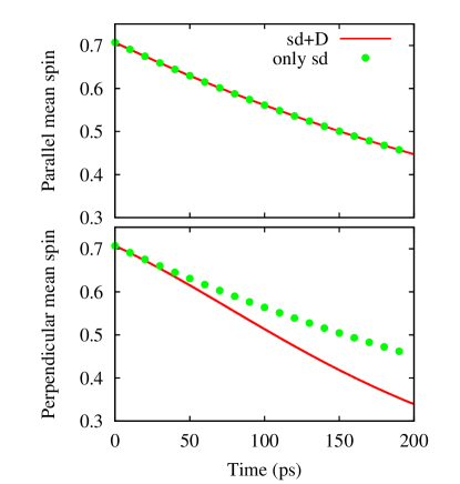
Figure 3: Influence of the Dresselhaus spin-orbit coupling (D) on the spin dynamics in bulk Zn_1-xMn_xSe with exchange $sd$-coupling (sd) for an initially Gaussian electron occupation centered at the band edge with standard deviation $\Delta=$3 meV and initial spin-polarization rotated 45 degrees with respect to the z-axis. The Mn concentration is $x_{\text{Mn}}=0.3\%$ and the net Mn magnetization $S=0.5$. Red solid lines correspond to the full calculation (sd+D) and green dotted lines to the calculation leaving out the Dresselhaus coupling (only sd).

This raises the question of whether a parameter regime can be reached experimentally in which the dephasing caused by the spin-orbit effective field has a considerable influence on or even dominates the spin dynamics. As mentioned above, shifting the optical excitation away from the band edge to higher k-values should enhance the effect of the SOI on the spin dynamics. Furthermore, the influence of the exchange $sd$-coupling can be reduced by lowering both the Mn concentration and/or the average Mn magnetization. Thus, in Fig. 4 we show the time evolution of the parallel and perpendicular spin components like in Fig. 3, but centering the Gaussian occupation 10 meV above the band edge and reducing the Mn magnetization to $S=0.1$. The Mn doping is kept at $x_{\text{Mn}}=0.3\%$ as before, and for the conduction-band electrons we choose again an initial spin orientation rotated 45 degrees away from the z-axis. In the parallel spin component there is now a noticeable difference between the full calculation (sd+D) (red solid line) and the sd-only case (green long-dashed line). A qualitatively new feature is that the combination of $sd$- and Dresselhaus couplings now produces not only a decay but also oscillations, revealing a combined spin precession. In the perpendicular component the spin-orbit coupling has now an enormous effect, greatly accelerating the decay and causing superimposed oscillations. The oscillations seen in Fig. 4 have a frequency close to the precession frequency associated with the mean Mn magnetic field ($\boldsymbol{\omega}_{\text{\tiny M}}=\omega_{\text{\tiny M}}\mathbf{\hat{z}}$), $\omega_{\text{\tiny M}}=0.124\,\text{Thz}$ (period $T_{\text{M}}=50.7\,\text{ps}$). We come back to this issue after discussing the mean-field approximation which we now introduce.

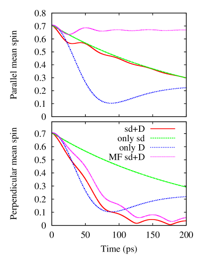
Figure 4: Influence of the Dresselhaus spin-orbit coupling (D) on the spin dynamics in bulk Zn_1-xMn_xSe with exchange $sd$-coupling (sd) for an initially Gaussian electron occupation centered at $E_{C}=$10 meV above the band edge with standard deviation $\Delta=$3 meV and initial spin-polarization rotated 45 degrees with respect to the z-axis. The Mn concentration is $x_{\text{Mn}}=0.3\%$ and the net Mn magnetization $S=0.1$. Red solid lines: full calculation with sd+D; green long-dashed lines: only sd; blue short-dashed: only D; pink dotted lines: mean-field approximation with sd+D.

It is interesting to elucidate whether a similar spin dynamics would also be obtained in a simpler scenario combining the Dresselhaus SOI with a constant magnetic field of appropriate strength. (This type of problem has been studied recently from the point of view of impurity entanglement met-dil-egg and spin relaxation zho-yu-wu .) We can readily answer this question by intentionally leaving the correlation terms out of the equations of motion [keeping in the RHS of Eq. (9) only the first term of the second line] thus reverting to a mean-field approximation, which for a given Mn magnetization is equivalent to adding a constant magnetic field. The result is given by the pink dotted lines in Fig. 4. For the perpendicular component we see that the mean-field calculation resembles the full one, although there is a clearly distinguishable difference between them. On the other hand, both results are far away from the $sd$-only result, and we have to conclude that in this sense the mean-field approximation does capture an important part of the interplay between the exchange and spin-orbit couplings. For the parallel component the mean-field approximation radically modifies the dynamics. We see here that when the $sd$ correlations are removed the spin-orbit dephasing is not capable by itself of inducing a decay in the presence of the spin precession about the Mn magnetization. In other words, the longitudinal component does not decay since its Dresselhaus dephasing is in a sense prevented by the ’naked’ (without exchange-induced correlations) precession about the Mn magnetization. To confirm this point we show in Fig. 4 the spin dynamics with only the Dresselhaus SOI (no $sd$-coupling) with blue dotted lines. These curves show the strong decay induced by spin-orbit dephasing in the absence of both the spin precession and the spin transfer caused by the exchange coupling.

The origin and frequency of the oscillations mentioned above, which appear when both interactions are present, and in both the full and mean-field calculations, can be interpreted with the help of Eq. (17). For a given $\mathbf{k}$-state the precession frequency is now $\mathbf{\Omega}\equiv\mathbf{\Omega}_{\mathbf{k}}+\omega_{\text{\tiny M}}\mathbf{z}$. In the limit $\omega_{\text{\tiny M}}\gg\Omega_{\mathbf{k}}$ we can assume that $\Omega_{z}\approx\Omega\approx\omega_{\text{\tiny M}}$, and using Eqs. (15) and (17) we obtain $\langle s_{z}\rangle(t)=\langle s_{z}\rangle(0)$. This argument applies to every $\mathbf{k}$-state and thus can be extended to the whole electron population. Then, the precession about the spin-orbit effective magnetic field of the longitudinal component is suppressed by the dominant precession about the Mn magnetic field, a feature that can be seen clearly in the mean-field result of Fig. 4. If the spin-orbit angular frequency is not completely neglected we obtain oscillations in the parallel component with frequency $|\mathbf{\Omega}_{\mathbf{k}}+\boldsymbol{\omega}_{\text{\tiny M}}|$ and small amplitude proportional to $1-(\Omega_{\mathbf{k},z}+\omega_{\text{\tiny M}})^{2}/|\mathbf{\Omega}_{\mathbf{k}}+\boldsymbol{\omega}_{\text{\tiny M}}|^{2}$, as seen in Fig. 4. We have verified that increasing the Dresselhaus coupling increases the amplitude of the oscillations (not shown here). Oscillations of the same frequency are also present in the perpendicular spin component.

IV Hg_1-x-yMn_xCd_yTe quantum wells

We now turn to the study of the influence of the spin-orbit coupling in II-VI semiconductor quantum wells. In this case the SOI that we consider is the Rashba coupling (R), which is present when the quantum-well confinement lacks inversion symmetry. As explained in the Introduction, the role of the spin-orbit coupling is conceptually similar in bulk and in quantum wells, since in both cases it can be thought of as a $\mathbf{k}$-dependent Zeeman Hamiltonian which induces global dephasing in an electron gas. However, quantum wells offer greater flexibility to control the SOI and also display high electron mobilities in high quality modulation-doped samples. High mobilities amount to longer momentum-scattering times and therefore to more coherent quantum dynamics.

In line with the bulk studies discussed above, we first tested the spin dynamics in Zn_1-xMn_xSe quantum wells. For realistic parameters for this material, it turned out that the Rashba coupling was too weak to modify the dynamics driven by the exchange $sd$-coupling. The root of this difficulty seems to be the large bandgap (about 2.8 eV) of ZnSe, which results in a small Rashba coupling constant. Thus for the quantum well calculations we looked for a family of materials with stronger and more controllable Rashba interaction. Hg_1-xMn_xTe is a good candidate since the energy gap $E_{g}$ of this ternary compound depends strongly on the Mn concentration,fur going to zero at $x\leq 6.5\%$, while its spin-orbit valence-band splitting $\Delta$ is insensitive to it.kos This interesting combination leads to flexible spin-orbit properties, which are generally controlled by the ratio $\Delta/E_{g}$. By choosing a Mn concentration slightly above $6.5\%$ we can select a very low energy gap, which leads in turn to a strong Rashba coupling.dea-lar-bas However, this lower limit for the Mn concentration is still too high and leads again to a completely dominant exchange interaction even for as low a Mn magnetization of $S=0.01$ (with $sd$-coupling induced spin relaxation times below 5 ps). This drawback can be overcome by considering instead the compound Hg_1-x-yMn_xCd_yTe in which the non-magnetic Cd atoms replace some of the Mn dopants. This change maintains the gap tunability via the doping fraction $x+y$ giving full flexibility regarding the concentration of magnetic ions.kos The Rashba coupling constant can be calculated with the expression dea-lar-bas ; gna-nav

$$\alpha_{R}=\frac{\hbar^{2}}{2m^{\ast}}\frac{\Delta}{E_{g}}\frac{2E_{g}+\Delta}{(E_{g}+\Delta)(3E_{g}+2\Delta)}\frac{V_{\text{qw}}}{d}\,.$$ (18)

We work with the effective mass of HgTe, $m^{\ast}=0.093\,m_{0}$,yu-car and take the spin-orbit valence-band splitting as $\Delta=1.08\,\text{eV}$.zhu-xia Assuming $E_{g}=300\,\text{meV}$, a quantum-well width $d=200\,\text{\AA}$, and a potential energy drop of $V_{\text{qw}}=50\,\text{meV}$ across the quantum well, we obtain $\alpha_{R}=4.87\,\text{meV}\,\text{nm}$ ($\alpha_{R}/\hbar=7.4\,\text{ps}^{-1}\text{nm}$). Note that for ZnSe one obtains $\alpha_{R}=0.015\,\text{meV}\,\text{nm}$ ($\alpha_{R}/\hbar=0.023\,\text{ps}^{-1}\text{nm}$), a very low value which leads to negligible spin-orbit effects, as mentioned before. For the exchange $sd$-coupling constant of HgMnTe we take $N_{0}\alpha=400\,\text{meV}$,liu-buh-nov and the lattice constant of $0.645\,\text{nm}$ leads to $J_{sd}=26.8\,\text{meV}\,\text{nm}^{3}$. We keep the previous Mn concentration of $x=0.3\%$.

In Fig. 5 we show the time evolution of the parallel and perpendicular spin components for quantum wells, where now the parallel component corresponds to the growth direction of the quantum well ($z$-axis). The Gaussian occupation is centered 10 meV above the band edge and we consider a Mn magnetization of $S=0.1$. The initial spin orientation is rotated 45 degrees away from the z-axis.

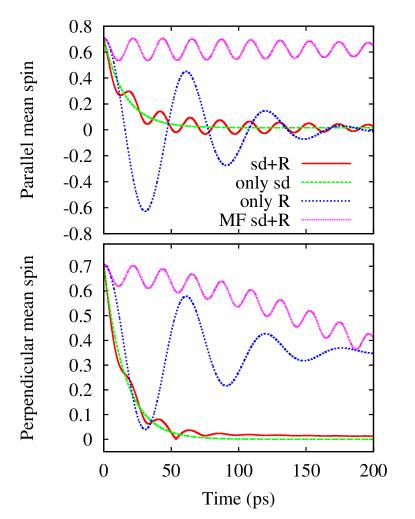
Figure 5: Influence of the Rashba spin-orbit coupling (R) on the spin dynamics in a Hg_1-x-yMn_xCd_yTe quantum well with exchange $sd$-coupling (sd) for an initially Gaussian electron occupation centered 10 meV above the band edge with standard deviation of 3 meV and initial spin-polarization rotated 45 degrees with respect to the z-axis. The Mn concentration is $x_{\text{Mn}}=0.3\%$ and the net Mn magnetization $S=0.1$. Red solid lines: full calculation with sd+R; green long-dashed lines: only sd; blue short-dashed lines: only R; pink dotted lines: mean-field approximation with sd+R.

Figure 5 shows that while the sd-only curve (green long-dashed line) follows the usual exponential decay, the full dynamics with sd+R displays clear oscillations in both components. We have verified that the amplitude of these oscillations increases with increasing Rashba coefficient, which in turn is obtained by lowering the energy gap. The pink-dotted-lines in Fig. 5 show the mean-field approximation results with both sd+R. Here the decay seen in the perpendicular component is due to the Rashba-induced dephasing since exchange correlations are absent. The parallel component maintains an approximately constant mean value in agreement with the analysis done in the previous Section, and shows a slight decrease of the oscillation amplitude due to the dephasing induced by the Rashba SOI. We verified that this amplitude reduction is accelerated by increasing the Rashba coupling constant. The blue-short-dashed lines show the evolution of the spin with only the Rashba interaction present (no sd). Here we see the full-fledged oscillations that had been anticipated in the discussion of Fig. 2. These oscillations are the collective result of the individual spin precessions about the effective $\mathbf{k}$-dependent Rashba magnetic field. To the best of our knowledge, an analytical expression or a simple interpretation for the frequency of these oscillations is not currently available. This frequency depends on many factors such as the Rashba coefficient, the electron density, and the electronic distribution (which in our simulations is determined by the mean value and the standard deviation of the initial Gaussian population). We have checked numerically that there is a roughly linear dependence of this frequency on the Rashba coefficient for an excitation 10 meV above the band edge.

It is unexpected and noteworthy that, in the quantum-well case, the addition of the spin-orbit interaction to the DMS produces strong oscillations while at the same time leaves fairly unchanged the decay rate for our parameters, as can be seen in Fig.  5 (“only sd” versus “sd+R” curves). Finally, we point out that the main qualitative difference between the results shown in Fig. 4 for bulk and Fig. 5 for a quantum well is that, for the perpendicular spin component in the quantum well, the sd-only curve stays near the full result and the MF curve moves strongly away, while the opposite behavior occurs in bulk.

V Conclusion

We studied theoretically the combined effects of the exchange $sd$-coupling and the spin-orbit interaction in II-VI diluted magnetic semiconductors (DMS), both in bulk and in quantum wells. Although our results can be considered generally valid in zincblende semiconductor systems, we focused on particular materials that show clearly the interplay between the two mechanisms: Zn_1-xMn_xSe for bulk and Hg_1-x-yMn_xCd_yTe for quantum wells. In our calculations we employed a recently developed formalism which incorporates electronic correlations originated from the exchange $sd$-coupling. The main conclusion of our study is that for both bulk and quasi-two-dimensional systems there can be a strong interplay or competition between the two types of interactions, leading to experimentally detectable signatures (for example in time-resolved Faraday and Kerr rotation experiments) of the spin-orbit interaction in DMS. In bulk we find that the spin components parallel and perpendicular to the net Mn magnetization have rather different responses to the presence of the spin-orbit (Dresselhaus) interaction, the latter being much more affected by it. Indeed, coherent oscillations—with a frequency reflecting the precession around a combination of the Mn magnetization and the Dresselhaus field—develop as a consequence of the interplay between the two interactions, which are completely absent when the exchange interaction dominates. In addition, the decay rate is greatly enhanced for the perpendicular component by the presence of the Dresselhaus interaction in the studied regime. Regarding quantum wells, we find that the exchange interaction tends to be more dominant over the spin-orbit interaction (Rashba coupling in this case), which led us to consider a family of materials with large valence-band-splitting spin-orbit constant and tunable energy gap. For these DMS materials we obtained again a strong effect of the spin-orbit interaction, manifesting itself in the occurence of oscillations which are not seen when the exchange interaction acts alone. Remarkably, even though the combination of exchange and spin-orbit interaction leads to clearly visible oscillations, the decay of the spin polarization is practically unaffected by the presence of the Rashba interaction. These signatures should be detectable experimentally in pump-and-probe experiments. Finally, for both bulk and quantum wells we find that in the mean-field approximation treatment of the exchange interaction there is a strong suppression of the spin-orbit-induced dephasing of the spin component parallel to the Mn magnetic field. The studied interplay between the spin-orbit interaction and the exchange coupling could improve spin control and thereby facilitate potential spintronic applications of DMS.

- (1) Introduction to the Physics of Diluted Magnetic Semiconductors, edited by Jacek Kossut and Jan A. Gaj (Springer, Heidelberg, 2010).
- (2) Semiconductor Spintronics, Jianbai Xia, Weikun Ge, and Kai Chang (World Scientific, Singapore, 2012).
- (3) A. Kirilyuk, A. V. Kimel, and T. Rasing, Rev. Mod. Phys. 82, 2731 (2010).
- (4) J. Qi, Y. Xu, A. Steigerwald, X. Liu, J. K. Furdyna, I. E. Perakis, and N. H. Tolk, Phys. Rev. B 79, 085304 (2009).
- (5) Y. Hashimoto, S. Kobayashi, and H. Munekata, Phys. Rev. Lett. 100, 067202 (2008).
- (6) L. Cywiński and L. J. Sham, Phys. Rev. B 76, 045205 (2007).
- (7) O. Morandi, P.-A. Hervieux, and G. Manfredi. Phys. Rev. B 81, 155309 (2010).
- (8) M. D. Kapetanakis, I. E. Perakis, K. J. Wickey, C. Piermarocchi, and J. Wang, Phys. Rev. Lett. 103, 047404 (2009).
- (9) C. Thurn, V. M. Axt, A. Winter, H. Pascher, H. Krenn, X. Liu, J. K. Furdyna, and T. Wojtowicz, Phys. Rev. B 80, 195210 (2009).
- (10) Spin-orbit coupling effects in two-dimensional electron and hole systems, R. Winkler (Springer-Verlag, Berlin, 2003).
- (11) I. Zutić, J. Fabian, and S. Das Sarma, Rev. Mod. Phys. 76, 323 (2004).
- (12) J. Fabian, A. Matos–Abiague, C. Ertler, P, Stano, and I. Žutić, Acta Physica Slovaca 57, 565 (2007).
- (13) Spin Physics in Semiconductors, edited by M. I. D’yakonov (Springer, Berlin, 2008).
- (14) M. W. Wu, J. H. Jiang, and M. Q. Weng, Physics Reports 493, 61 (2010).
- (15) Handbook of Spin Transport and Magnetism, edited by E. Y. Tsymbal and I. Žutić (Chapman & Hall/CRC, Boca Raton, FL, 2011).
- (16) K. Gnanasekar and K. Navaneethakrishnan, Physica E 35, 103–109 (2006).
- (17) W. Yang, Kai Chang, X. G. Wu, H. Z. Zheng, and F. M. Peeters, Appl. Phys. Lett. 89, 132112 (2006).
- (18) R. Vali and S. M. Mirzanian, Solid State Comm. 49, 2032–2035(2009).
- (19) J. H. Jiang, Y. Zhou, T. Korn, C. Schüller, and M. W. Wu, Phys. Rev. B 79, 155201 (2009).
- (20) S. M. Mirzanian, A. A. Shokri, and S. M. Elahi, J. Mater. Sci. 49, 88–93 (2014).
- (21) K. S. Denisov and N. S. Averkiev, JETP Letters 99, 400–404 (2014).
- (22) A. Manchon and S. Zhang, Phys. Rev. B 79, 094422 (2009).
- (23) I. Garate and A. H. MacDonald, Phys. Rev. B 80, 134403 (2009).
- (24) K. M. D. Hals, A. Brataas, and Y. Tserkovnyak, Eur. Phys. Lett. 90, 47002 (2010).
- (25) A. Chernyshov, M. Overby, X. Liu, J. K. Furdyna, Y. Lyanda-Geller, and L. P. Rokhinson, Nat. Phys. 5, 656 (2009).
- (26) M. Endo, F. Matsukura, and H. Ohno, Appl. Phys. Lett. 97, 222501 (2010).
- (27) D. Fang, H. Kurebayashi, J. Wunderlich, K. Výborný, L. P. Zârbo, R. P. Campion, A. Casiraghi, B. L. Gallagher, T. Jungwirth, and A. J. Ferguson, Nat. Nanotechnol. 6, 413 (2011).
- (28) H. Li, X. Wang, F. Doan, and A. Manchon, Appl. Phys. Lett. 102, 192411 (2013).
- (29) P. C. Lingos, J. Wang, and I. E. Perakis, arXiv:1411.6662v1 [cond-mat.str-el] 24 Nov 2014.
- (30) C. Thurn and V. M. Axt, Phys. Rev. B 85, 165203 (2012).
- (31) M. Cygorek and V. M. Axt, arXiv:1412.5898v1 [cond-mat.mes-hall] 18 Dec 2014.
- (32) Spin Physics in Semiconductors, J. D. Cibert and D. Scalbert (Springer, Heidelberg, 2008), chapter 13.
- (33) G. Dresselhaus, Phys. Rev. B 100, 580 (1955).
- (34) E. I. Rashba, Sov. Phys. Solid State 2, 1109 (1960). Y. A. Bychkov and E. I. Rashba, JETP Lett. 39, 78 (1984); J. Phys. C 17, 6039 (1984).
- (35) M. Cygorek and V. M. Axt, Phys. Rev. B 90, 035206 (2014).
- (36) Semiconductors and Semimetals, volume 25, J. K. Furdyna and J. Kossut, Editors (Academic Press, San Diego, CA, 1988).
- (37) C. Thurn, M. Cygorek, V. M. Axt, and T. Kuhn, Phys. Rev. B 88, 161302(R) (2013)
- (38) C. Thurn, M. Cygorek, V. M. Axt, and T. Kuhn, Phys. Rev. B 87, 205301 (2013).
- (39) M. I. D’yakonov and V. I. Perel, Sov. Phys. JETP 33, 1053 (1971).
- (40) Fundamentals of Semiconductors, Fourth Edition, P. Y. Yu and M. Cardona (Springer, Heidelberg, 2010).
- (41) A. Twardowski, M. von Ortenberg, M. Demianiuk, and R. Pauthenet, Solid State Commun. 51, 849 (1984).
- (42) B. König, I. A. Merkulov, D. R. Yakovlev, W. Ossau, S. M. Ryabchenko, M. Kutrowski, T. Wojtowicz, G. Karczewski, and J. Kossut, Phys. Rev. B 61, 16870 (2000).
- (43) A. Metavitsiadis, R. Dillenschneider, and S. Eggert, Phys. Rev. B 89, 155406 (2014).
- (44) Y. Zhou, T. Yu, and M. W. Wu, Phys. Rev. B 87, 245304 (2013).
- (45) J. Furdyna, J. Appl. Phys. 64, R29 (1988).
- (46) J. Kossut, Band structure and Quantum Transport Phenomena in Narrow-Gap Diluted Magnetic Semiconductors, chapter 5 in Semiconductors and Semimetals, volume 25, J. K. Furdyna and J. Kossut, Editors (Academic Press, San Diego, CA, 1988).
- (47) E. A. de Andrada e Silva, G. C. La Rocca and F. Bassani, Phys. Rev. B 55, 16293 (1997).
- (48) Y.-H. Zhu and J.-B. Xia, EPL 82, 37004 (2008). O. Madelung, M. Schulz, and H. Weiss (Editors), Physics of II-VI and I-VII Compounds, Semimagnetic Semiconductors, Landolt-Börnstein, New Ser., Group III, Vol. 17, Part b (Springer-Verlag, Berlin, 1982).
- (49) Jian Liu, H. Buhmann, E. G. Novik, Yongsheng Gui, V. Hock, C. R. Becker, and L. W. Molenkamp, Phys. Stat. Sol. (b) 243, 835-838 (2006).