Linear Global Translation Estimation
with Feature Tracks

Abstract

This paper derives a novel linear position constraint for cameras seeing a common scene point, which leads to a direct linear method for global camera translation estimation. Unlike previous solutions, this method deals with collinear camera motion and weak image association at the same time. The final linear formulation does not involve the coordinates of scene points, which makes it efficient even for large scale data. We solve the linear equation based on $L_{1}$ norm, which makes our system more robust to outliers in essential matrices and feature correspondences. We experiment this method on both sequentially captured images and unordered Internet images. The experiments demonstrate its strength in robustness, accuracy, and efficiency.

1 Introduction

Structure-from-motion (SfM) algorithms aim to estimate scene structure and camera motion from multiple images, and they can be broadly divided into incremental and global methods according to their ways to register cameras. Incremental methods register cameras one by one [Snavely et al.(2006)Snavely, Seitz, and Szeliski, Wu(2013)] or iteratively merge partial reconstructions [Fitzgibbon and Zisserman(1998), Lhuillier and Quan(2005)]. These methods require frequent intermediate bundle adjustment (BA) to ensure correct reconstruction, which is computationally expensive. Yet, their results often suffer from large drifting errors. In comparison, global methods (e.g[Govindu(2001), Martinec and Pajdla(2007), Crandall et al.(2011)Crandall, Owens, Snavely, and Huttenlocher, Jiang et al.(2013)Jiang, Cui, and Tan, Wilson and Snavely(2014), Özyesil and Singer(2015)]) register all cameras simultaneously, which has better potential in both efficiency and accuracy.

\begin{overpic}[width=390.25534pt,tics=10]{./BMVC_Introduction3.pdf} \par\put(5.0,125.0){\rotatebox{90.0}{\small\emph{Street}}} \put(5.0,40.0){\rotatebox{90.0}{\small\emph{Seville}}} \par\put(100.0,90.0){\small Result from \cite[cite]{[\@@bibref{}{Wilson2014}{}{}]}} \put(250.0,90.0){\small Our result} \par\put(100.0,-6.0){\small Result from \cite[cite]{[\@@bibref{}{jiang2013g}{}{}]}} \put(250.0,-6.0){\small Our result} \par\end{overpic}

Figure 1: 1DSFM [Wilson and Snavely(2014)] and triplet-based methods (e.g[Jiang et al.(2013)Jiang, Cui, and Tan]) require strong association among images. As shown in the left, they fail for images with weak association. In comparison, as shown in the right, the results from our method do not suffer from such problems.

Global SfM methods often solve the camera orientations and positions separately. The global position estimation is more challenging than the orientation estimation due to the noisy pairwise translation encoded in essential matrices [Enqvist et al.(2011)Enqvist, Kahl, and Olsson]. This paper focuses on the problem of global position (i.etranslation) estimation.

Essential matrix based translation estimation methods [Govindu(2001), Brand et al.(2004)Brand, Antone, and Teller, Arie-Nachimson et al.(2012)Arie-Nachimson, Kovalsky, Kemelmacher-Shlizerman, Singer, and Basri] can only determine camera positions in a parallel rigid graph [Özyesil and Singer(2015)], and they usually degenerate at collinear camera motion because the translation scale is not determined by an essential matrix. Trifocal tensor based methods [Sim and Hartley(2006), Courchay et al.(2010)Courchay, Dalalyan, Keriven, and Sturm, Moulon et al.(2013)Moulon, Monasse, and Marlet, Jiang et al.(2013)Jiang, Cui, and Tan] could deal with collinear motion as the relative scales are encoded in a trifocal tensor. However, these methods usually rely on a strongly connected camera-triplet graph, where two triplets are connected by their common edge. The 3D reconstruction will distort or break into disconnected components when such strong association among images does not exist. By solving cameras and scene points together, some global methods [Rother(2003), Kahl and Hartley(2007), Martinec and Pajdla(2007), Crandall et al.(2011)Crandall, Owens, Snavely, and Huttenlocher, Sinha et al.(2010)Sinha, Steedly, and Szeliski] can deal with collinear motion. These methods usually need to filter epipolar geometries (EGs) carefully to avoid outliers. Including scene points in the formulation also hurts the scalability of the algorithm, since there are many more scene points than cameras. The recent 1DSfM method [Wilson and Snavely(2014)] designs a smart filter to discard outlier essential matrices and solves scene points and cameras together by enforcing orientation consistency. However, this method requires abundant association between input images, e.g$\sim O(n^{2})$ essential matrices for $n$ cameras, which is more suitable for Internet images and often fails on sequentially captured data.

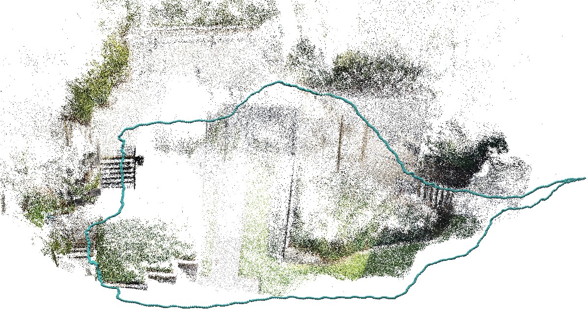
The data association problem of 1DSfM [Wilson and Snavely(2014)] and triplet-based methods (here, we take [Jiang et al.(2013)Jiang, Cui, and Tan] as an example) is exemplified in Figure 1. The Street example on the top is a sequential data. 1DSfM fails on this example due to insufficient image association, since each image is only matched to its 4 neighbors at the most. In the Seville example on the bottom, those Internet images are mostly captured from two viewpoints (see the two representative sample images) with weak affinity between images at different viewpoints. This weak data association causes seriously distorted reconstruction for the triplet-based method in [Jiang et al.(2013)Jiang, Cui, and Tan].

This paper introduces a direct linear algorithm to address the presented challenges. It avoids degeneracy at collinear motion and deals with weakly associated data. Our method capitalizes on constraints from essential matrices and feature tracks. For a scene point visible in multiple (at least three) cameras, we consider triangles formed by this scene point and two camera centers. We first generalize the camera-triplet based position constraint in [Jiang et al.(2013)Jiang, Cui, and Tan] to our triangles with scene points. We then eliminate the scene point from these constraints. In this way, we obtain a novel linear equation for the positions of cameras linked by a feature track. Solving these linear equations from many feature tracks simultaneously register all cameras in a global coordinate system.

This direct linear method minimizes a geometric error, which is the Euclidean distance between the scene point to its corresponding view rays. It is more robust than the linear constraint developed in [Rother(2003)], which minimizes an algebraic error. A key finding in this paper is that, a direct linear solution (without involving scene points) exists by minimizing the point-to-ray error instead of the reprojection error. Since the point-to-ray error approximates the reprojection error well when cameras are calibrated, our method is a good linear initialization for the final nonlinear BA.

At the same time, this direct linear formulation lends us sophisticated optimization tools, such as $L_{1}$ norm optimization [Candes and Tao(2005), Goldstein and Osher(2009), Boyd et al.(2011)Boyd, Parikh, Chu, Peleato, and Eckstein, Parikh and Boyd(2013)]. We minimize the $L_{1}$ norm when solving the linear equation of camera positions. In this way, our method can tolerate a larger amount of outliers in both essential matrices and feature correspondences. The involved $L_{1}$ optimization is nontrivial. We derive a linearization of the alternating direction method of multipliers algorithm [Boyd et al.(2011)Boyd, Parikh, Chu, Peleato, and Eckstein] to address it.

2 Related Work

Incremental approaches. Most of well-known SfM systems register cameras sequentially [Pollefeys et al.(2004)Pollefeys, Van Gool, Vergauwen, Verbiest, Cornelis, Tops, and Koch, Snavely et al.(2006)Snavely, Seitz, and Szeliski, Snavely et al.(2008)Snavely, Seitz, and Szeliski, Pollefeys et al.(2008)Pollefeys, Nistér, Frahm, Akbarzadeh, Mordohai, Clipp, Engels, Gallup, Kim, Merrell, et al., Agarwal et al.(2009)Agarwal, Snavely, Simon, Seitz, and Szeliski] or hierarchically [Fitzgibbon and Zisserman(1998), Lhuillier and Quan(2005), Havlena et al.(2009)Havlena, Torii, Knopp, and Pajdla] from pairwise relative motions. In order to minimize error accumulation, frequent intermediate bundle adjustment is required for both types of methods, which significantly reduces computation efficiency. The performance of sequential methods relies heavily on the choice of the initial image pair and the order of subsequent image additions [Haner and Heyden(2012)].

Global rotation estimation. Global SfM methods solve all camera poses simultaneously. Most of these methods take two steps. Typically, they solve camera orientations first and then positions. The orientation estimation is well studied with an elegant rotation averaging algorithm presented in [Hartley et al.(2013)Hartley, Trumpf, Dai, and Li]. The basic idea was first introduced by Govindu [Govindu(2001)], and then developed in several following works [Govindu(2004), Martinec and Pajdla(2007), Hartley et al.(2013)Hartley, Trumpf, Dai, and Li]. In particular, [Chatterjee and Govindu(2013)] introduced a robust $L_{1}$ method which was adopted in several recent works [Wilson and Snavely(2014), Özyesil and Singer(2015)].

Global translation estimation. The translation estimation is more challenging. Some pioneer works [Govindu(2001), Brand et al.(2004)Brand, Antone, and Teller, Govindu(2006), Arie-Nachimson et al.(2012)Arie-Nachimson, Kovalsky, Kemelmacher-Shlizerman, Singer, and Basri] solved camera positions solely from constraints in essential matrices. Typically, they enforce consistency between pairwise camera translation directions and those encoded in essential matrices. Recently, Özyesil and Singer [Özyesil and Singer(2015)] prove that essential matrices only determine camera positions in a parallel rigid graph, and present a convex optimization algorithm to solve this problem. In general, all these essential matrix based methods degenerate at collinear motion, where cameras are not in a parallel rigid graph.

This degeneracy can be avoided by exploiting relative motion constraints from camera triplets [Sim and Hartley(2006), Courchay et al.(2010)Courchay, Dalalyan, Keriven, and Sturm, Sinha et al.(2010)Sinha, Steedly, and Szeliski, Moulon et al.(2013)Moulon, Monasse, and Marlet], as the trifocal tensor encodes the relative scale information. Recently, Jiang et al. [Jiang et al.(2013)Jiang, Cui, and Tan] derived a novel linear constraint in a camera triplet and solved all cameras positions in a least square sense. While triplet-based methods avoid degenerated camera motion, they often require strong association among images – a connected triplet graph, where camera triplets are connected by common edges.

Some global methods estimate cameras and scene points together. Rother [Rother(2003)] solved camera positions and points by minimizing an algebraic error. Some works [Kahl and Hartley(2007), Martinec and Pajdla(2007), Olsson et al.(2007)Olsson, Eriksson, and Kahl, Agarwal et al.(2008)Agarwal, Snavely, and Seitz, Li(2009)] solved the problem by minimizing the $L_{\infty}$ norm of reprojection error. However, the $L_{\infty}$ norm is known to be sensitive to outliers and careful outlier removal is necessary [Olsson et al.(2010)Olsson, Eriksson, and Hartley, Dalalyan and Keriven(2009)]. Recently, Wilson and Snavely [Wilson and Snavely(2014)] directly solved cameras and points by Ceres Solver [Agarwal et al.()Agarwal, Mierle, and Others] after applying a smart filter to essential matrices. Generally speaking, involving scene points improves the robustness/accuracy of camera registration, but also significantly increases the problem scale. Feature correspondence outliers also pose a significant challenge for these methods.

Our method capitalizes on constraints in essential matrices and feature tracks. It avoids degeneracy at collinear motion, handles weak data association, and is robust to feature correspondence outliers.

3 Global Translation Estimation

Given an essential matrix between two images $i,j$ (e.gcomputed by the five-point algorithm [Nistér(2004), Li and Hartley(2006)]), we obtain the relative rotation $\mbox{{\bf R}}_{ij}$ and translation direction $\mbox{{\bf t}}_{ij}$ between the two cameras. Here, $\mbox{{\bf R}}_{ij}$ is a $3\times 3$ orthonormal matrix and $\mbox{{\bf t}}_{ij}$ is a $3\times 1$ unit vector. We further denote the global orientation and position of the $i$-th ($1\leq i\leq N$) camera as $\mbox{{\bf R}}_{i}$ and $\mbox{{\bf c}}_{i}$ respectively. These camera poses are constrained by the following equations

$$\mbox{{\bf R}}_{j}=\mbox{{\bf R}}_{ij}\mbox{{\bf R}}_{i},\ \ \ \ \mbox{{\bf R}}_{j}(\mbox{{\bf c}}_{i}-\mbox{{\bf c}}_{j})\simeq\mbox{{\bf t}}_{ij}.$$ (1)

Here, $\simeq$ means equal up to a scale.

Like most global methods, we compute camera orientations first and solve camera positions after that. We adopt the global rotation estimation method in [Chatterjee and Govindu(2013)]. In order to enhance robustness, we adopt additional loop verifications [Zach et al.(2010)Zach, Klopschitz, and Pollefeys] on the input pairwise relative camera rotations beforehand. Specifically, we chain the relative rotations along a three-camera loop as $\hat{\mbox{{\bf R}}}=\mbox{{\bf R}}_{ij}\mbox{{\bf R}}_{jk}\mbox{{\bf R}}_{ki}$, and compute the angular difference [Hartley et al.(2013)Hartley, Trumpf, Dai, and Li] between $\hat{\mbox{{\bf R}}}$ and the identity matrix. If the difference is larger than a threshold $\varphi_{1}$ ($3$ or $5$ degrees for sequential data or unordered Internet data), we consider the verification fails. We discard an EG if every verification it participates in fails.

The key challenge in translation estimation is that an essential matrix does not tell the scale of translation. We seek to obtain linear equations for those unknown scales without resorting to camera-triplets. Our translation estimation is based on a linear position constraint arising from a triangle formed by two camera positions and a scene point. With this constraint, the positions of cameras linked by a feature point should satisfy a linear equation.

(a)	(b)

Figure 2: (a) The positions of a scene point p and two camera centers $\mbox{{\bf c}}_{i}$ and $\mbox{{\bf c}}_{j}$ satisfy a linear constraint detailed in Section 3.1. (b) The positions of four cameras seeing the same scene point satisfy a linear constraint detailed in Section 3.2.

3.1 Constraints from a triangle

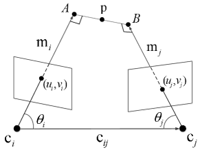
A linear constraint on positions of cameras in a triplet is derived in [Jiang et al.(2013)Jiang, Cui, and Tan]. We generalize it to the case of triangles formed by a scene point and two cameras. As shown in Figure 2, we compute the location of a scene point p as the middle point of the mutual perpendicular line segment $AB$ of the two rays passing through p’s image projections. Specifically, it is computed as

$$\vspace{-0.02in}\mbox{{\bf p}}=\frac{1}{2}(A+B)=\frac{1}{2}(\mbox{{\bf c}}_{i}+s_{i}\mbox{{\bf m}}_{i}+\mbox{{\bf c}}_{j}+s_{j}\mbox{{\bf m}}_{j}).$$ (2)

Here, $\mbox{{\bf c}}_{i}$ and $\mbox{{\bf c}}_{j}$ are the two camera centers. The two unit vectors $\mbox{{\bf m}}_{i}$ and $\mbox{{\bf m}}_{j}$ origin from the camera centers and point toward the image projections of p. $s_{i}$ and $s_{j}$ are the distances from the points $A,B$ to $\mbox{{\bf c}}_{i},\mbox{{\bf c}}_{j}$ respectively, i.e$A=\mbox{{\bf c}}_{i}+s_{i}\mbox{{\bf m}}_{i}$ and $B=\mbox{{\bf c}}_{j}+s_{j}\mbox{{\bf m}}_{j}$.

The rotation trick. The rotation trick used in [Jiang et al.(2013)Jiang, Cui, and Tan] shows that we can compute $\mbox{{\bf m}}_{i}$ and $\mbox{{\bf m}}_{j}$ by rotating the relative translation direction $\mbox{{\bf c}}_{ij}$ between $\mbox{{\bf c}}_{i}$ and $\mbox{{\bf c}}_{j}$, i.e$\mbox{{\bf m}}_{i}=\mbox{{\bf R}}(\theta_{i})\mbox{{\bf c}}_{ij}$ and $\mbox{{\bf m}}_{j}=-\mbox{{\bf R}}(\theta_{j})\mbox{{\bf c}}_{ij}$. Then Equation 2 becomes

$$\small\vspace{-0.02in}\mbox{{\bf p}}=\frac{1}{2}\left(\mbox{{\bf c}}_{i}+s_{i}\mbox{{\bf R}}(\theta_{i})\frac{\mbox{{\bf c}}_{j}-\mbox{{\bf c}}_{i}}{\left\|\mbox{{\bf c}}_{j}-\mbox{{\bf c}}_{i}\right\|}+\mbox{{\bf c}}_{j}+s_{j}\mbox{{\bf R}}(\theta_{j})\frac{\mbox{{\bf c}}_{i}-\mbox{{\bf c}}_{j}}{\left\|\mbox{{\bf c}}_{i}-\mbox{{\bf c}}_{j}\right\|}\right).$$ (3)

The two 3D rotation matrices $\mbox{{\bf R}}(\theta_{i})$ and $\mbox{{\bf R}}(\theta_{j})$ rotate the relative translation direction $\mbox{{\bf c}}_{ij}$ to the directions $\mbox{{\bf m}}_{i}$ and $\mbox{{\bf m}}_{j}$. Both rotations can be computed easily in the local pairwise reconstruction. In addition, the two ratios $s_{i}/\left\|\mbox{{\bf c}}_{j}-\mbox{{\bf c}}_{i}\right\|$ and $s_{j}/\left\|\mbox{{\bf c}}_{j}-\mbox{{\bf c}}_{i}\right\|$ can be computed by the middle-point algorithm [Hartley and Zisserman(2003)]. Specifically, assuming unit baseline length, in the local coordinate system attached to one of the cameras, $\mbox{{\bf c}}_{i},\mbox{{\bf c}}_{j}$, $\mbox{{\bf m}}_{i}$, and $\mbox{{\bf m}}_{j}$ are all known. Thus, we can solve $s_{i}$ and $s_{j}$ (they are actually the two ratios in Equation 3 for general baseline length) from

$$\vspace{-0.02in}(\mbox{{\bf c}}_{i}+s_{i}\mbox{{\bf m}}_{i}-\mbox{{\bf c}}_{j}-s_{j}\mbox{{\bf m}}_{j})\times(\mbox{{\bf m}}_{i}\times\mbox{{\bf m}}_{j})=0.$$ (4)

Here, $\times$ is the cross product of vectors. Thus, Equation 3 becomes,

$$\vspace{-0.02in}\mbox{{\bf p}}=\frac{1}{2}\left((\mbox{{\bf A}}_{j}^{ij}-\mbox{{\bf A}}_{i}^{ij})(\mbox{{\bf c}}_{i}-\mbox{{\bf c}}_{j})+\mbox{{\bf c}}_{i}+\mbox{{\bf c}}_{j}\right)$$ (5)

where $\mbox{{\bf A}}_{i}^{ij}=s_{i}/||\mbox{{\bf c}}_{j}-\mbox{{\bf c}}_{i}||\mbox{{\bf R}}(\theta_{i})$ and $\mbox{{\bf A}}_{j}^{ij}=s_{j}/||\mbox{{\bf c}}_{i}-\mbox{{\bf c}}_{j}||\mbox{{\bf R}}(\theta_{j})$ are known matrices. This equation provides a linear constraint among positions of two camera centers and a scene point. Note this linear constraint minimizes a geometric error, the point-to-ray distance.

3.2 Constraints from a feature track

If the same scene point p is visible in two image pairs $\mbox{{\bf c}}_{i},\mbox{{\bf c}}_{j}$ and $\mbox{{\bf c}}_{k},\mbox{{\bf c}}_{l}$ as shown in Figure 2 (b), we obtain two linear equations about p’s position according to Equation 5. We can eliminate p from these equations to obtain a linear constraint among four camera centers as the following,

$$\vspace{-0.02in}(\mbox{{\bf A}}_{j}^{ij}-\mbox{{\bf A}}_{i}^{ij})(\mbox{{\bf c}}_{i}-\mbox{{\bf c}}_{j})+\mbox{{\bf c}}_{i}+\mbox{{\bf c}}_{j}=(\mbox{{\bf A}}_{l}^{kl}-\mbox{{\bf A}}_{k}^{kl})(\mbox{{\bf c}}_{k}-\mbox{{\bf c}}_{l})+\mbox{{\bf c}}_{k}+\mbox{{\bf c}}_{l}.$$ (6)

Given a set of images, we build feature tracks and collect such linear equations from camera pairs on the same feature track. Solving these equations will provide a linear global solution of camera positions. To resolve the gauge ambiguity, we set the orthocenter of all cameras at origin when solving these equations.

Equation 6 elegantly correlates the scales of translation (i.ebaseline length$\left\|\mbox{{\bf c}}_{i}-\mbox{{\bf c}}_{j}\right\|$ and $\left\|\mbox{{\bf c}}_{k}-\mbox{{\bf c}}_{l}\right\|$) for camera pairs sharing a common scene point. For example, in the Seville data in Figure 1 (bottom row), $\mbox{{\bf c}}_{i},\mbox{{\bf c}}_{j}$ could come from one popular viewpoint of the building, and $\mbox{{\bf c}}_{k},\mbox{{\bf c}}_{l}$ could come from a different viewpoint. As long as there is a feature track linking them together, Equation 6 provides constraints among the baseline lengths of these far apart cameras. In comparison, triplet-based methods (e.g[Sim and Hartley(2006), Jiang et al.(2013)Jiang, Cui, and Tan, Moulon et al.(2013)Moulon, Monasse, and Marlet]) can only propagate the scale information over camera triplets sharing an edge. Clearly, the scale information can propagate further along feature tracks. Therefore, this new formulation can reconstruct images with weak association better than triplet-based methods.

3.3 Feature tracks selection

Since there are usually abundant feature tracks to solve camera positions, we carefully choose the most reliable ones to enhance system robustness. For better feature matching quality, we only consider feature correspondences that are inliers of essential matrix fitting. We sort all feature tracks by their lengths in descending order, and then try to find a small set of tracks that could cover all connected cameras at least $K$ times. (We set $K=30$ in our experiments.) Please see our supplementary material for the pseudo-code of the feature tracks selection.

For a feature track with $N_{t}$ cameras, there are usually more than $N_{t}-1$ EGs on it. So we select the most reliable ones to construct equations. We consider the match graph formed by these cameras, where two cameras are connected when their essential matrix is known. Since we only consider feature correspondences passing essential matrix verification, this graph has only one connected component. We weight each graph edge by $\frac{1}{M}+\alpha\frac{1}{\theta}$, where $M$ is the number of feature matches between two images, and $\theta$ is the triangulation angle. The combination weight $\alpha$ is fixed at $0.1$ in our experiments. We take the minimum spanning tree of this graph, and randomly choose two edges from the tree to build a linear equation until each edge is used twice.

4 Robust Estimation by $L_{1}$ Norm

Our linear global method requires solving a linear system like $\mbox{{\bf A}}\mbox{{\bf x}}=0$ to estimate camera centers. x represents an unknown vector formed by concatenating all camera positions, and A is the coefficient matrix formed by collecting Equation 6 from feature tracks.

The 3D reconstruction process is noisy and involves many outliers, both in essential matrices and feature correspondences. We enhance system robustness by minimizing the $L_{1}$ norm, instead of the conventional $L_{2}$ norm. In other words, we solve the following optimization problem,

$$\vspace{-0.02in}\arg\min_{\mbox{{\bf x}}}\left\|\mbox{{\bf A}}\mbox{{\bf x}}\right\|_{1},\qquad s.t.\quad\mbox{{\bf x}}^{\top}\mbox{{\bf x}}=1.$$ (7)

This problem might be solved by iterative reweighted total least squares, which is often slow and requires good initialization. Recently, Ferraz et al[Ferraz et al.(2014)Ferraz, Binefa, and Moreno-Noguer] proposed a robust method to discard outliers, while it is not applicable to our large sparse homogeneous system. We capitalize on the recent alternating direction method of multipliers (ADMM) [Boyd et al.(2011)Boyd, Parikh, Chu, Peleato, and Eckstein] for better efficiency and large convergence region. Due to the quadratic constraint, i.e$\mbox{{\bf x}}^{\top}\mbox{{\bf x}}=1$, the original ADMM algorithm cannot be directly applied to our problem. We linearize the optimization problem in the inner loop of ADMM to solve Equation 7.

Let $\mbox{{\bf e}}=\mbox{{\bf A}}\mbox{{\bf x}}$, the augmented Lagrangian function of Equation 7 is

$$L(\mbox{{\bf e}},\mbox{{\bf x}},\lambda)=\left\|\mbox{{\bf e}}\right\|_{1}+\left\langle\lambda,\mbox{{\bf A}}\mbox{{\bf x}}-\mbox{{\bf e}}\right\rangle+\frac{\beta}{2}\left\|\mbox{{\bf A}}\mbox{{\bf x}}-\mbox{{\bf e}}\right\|^{2},~{}~{}~{}~{}~{}~{}~{}s.t.\qquad\mbox{{\bf x}}^{\top}\mbox{{\bf x}}=1,$$ (8)

where $\lambda$ is the Lagrange multiplier, $\left\langle\cdot,\cdot\right\rangle$ is the inner product, and $\beta>0$ is a parameter controlling the relaxation.

We then iteratively optimize e, x, and $\lambda$ in Equation 8. In each iteration, we update $\mbox{{\bf e}}_{k+1}$, $\mbox{{\bf x}}_{k+1}$, $\lambda_{k+1}$ according to the following scheme,

$$\small\mbox{{\bf e}}_{k+1} = \arg\min_{\mbox{{\bf e}}}L(\mbox{{\bf e}},\mbox{{\bf x}}_{k},\lambda_{k})=\arg\min_{\mbox{{\bf e}}}\left\|\mbox{{\bf e}}\right\|_{1}+\left\langle\lambda_{k},\mbox{{\bf A}}\mbox{{\bf x}}_{k}-\mbox{{\bf e}}\right\rangle+\frac{\beta}{2}\left\|\mbox{{\bf A}}\mbox{{\bf x}}_{k}-\mbox{{\bf e}}\right\|^{2},$$ (9)

$$\mbox{{\bf x}}_{k+1} = \arg\min_{\mbox{{\bf x}}\in\Omega}L(\mbox{{\bf e}}_{k+1},\mbox{{\bf x}},\lambda_{k})=\arg\min_{\mbox{{\bf x}}\in\Omega}\left\langle\lambda_{k},\mbox{{\bf A}}\mbox{{\bf x}}-\mbox{{\bf e}}_{k+1}\right\rangle+\frac{\beta}{2}\left\|\mbox{{\bf A}}\mbox{{\bf x}}-\mbox{{\bf e}}_{k+1}\right\|^{2},$$ (10)

$$\lambda_{k+1} = \lambda_{k}+\beta(\mbox{{\bf A}}\mbox{{\bf x}}_{k+1}-\mbox{{\bf e}}_{k+1}),$$ (11)

where $\Omega:=\left\{\mbox{{\bf x}}^{\top}\mbox{{\bf x}}=1|\mbox{{\bf x}}\in\mathbb{R}^{n}\right\}$. A closed-form solution [Lin et al.(2010)Lin, Chen, and Ma] exists for the minimization of Equation 9. (Please see Appendix A for the formula.) Solving Equation 10 is hard because of the quadratic constraint on x. Therefore, we linearize Equation 10 and derive a closed-form solution as,

$$\vspace{-0.025in}\mbox{{\bf x}}_{k+1}=C/\left\|C\right\|^{2},$$ (12)

where $C=\mbox{{\bf x}}_{k}-\frac{1}{\eta}\mbox{{\bf A}}^{\top}(\mbox{{\bf A}}\mbox{{\bf x}}_{k}-\mbox{{\bf e}}_{k+1})-\frac{1}{\beta\eta}\mbox{{\bf A}}^{\top}\lambda^{k}$, and $\eta>\sigma_{max}(\mbox{{\bf A}}^{\top}\mbox{{\bf A}})$. (Please see Appendix B for more details.) In order to speed up convergence [Lin et al.(2011)Lin, Liu, and Su], we adopt a dynamic parameter $\beta$ as,

$$\vspace{-0.025in}\beta_{k+1}=min{\left\{\beta_{max},\rho\beta_{k}\right\}},$$ (13)

where $\rho>1$. We set $\rho$ as $1.01$ or $1.1$ for sequential data and Internet data respectively in our experiments. Algorithm 1 summarizes our linearized ADMM algorithm.

Algorithm 1 Our linearized ADMM for Equation 7.

1:Initialize: Set $\mbox{{\bf x}}_{0}$ as to the $L_{2}$ solution (i.ethe eigenvector with smallest eigenvalue of A), $\mbox{{\bf e}}_{0}=\mathbf{0}$, $\lambda_{0}=\mathbf{0}$, $\beta_{0}=10^{-6}$;

2:while not converged, do

3:     Step 1: Update e by solving Equation 9;

4:     Step 2: Update x by solving Equation 12;

5:     Step 3: Update $\lambda$ by solving Equation 11;

6:     Step 4: Update $\beta$ by solving Equation 13;

7:end while

5 Experiments

Dataset	$c_{err}$ (GT,mm)
	Rother[Rother(2003)]	Jiang[Jiang et al.(2013)Jiang, Cui, and Tan]	Moulon[Moulon et al.(2013)Moulon, Monasse, and Marlet]	Arie[Arie-Nachimson et al.(2012)Arie-Nachimson, Kovalsky, Kemelmacher-Shlizerman, Singer, and Basri]	VisualSFM[Wu(2013)]	1DSfM[Wilson and Snavely(2014)]	$L_{2}$	$L_{1}$
fountain-P11	2.5	3.1	2.5	2.9	3.6	33.5	2.5	2.5
Herz-Jesu-P25	5.0	7.5	5.3	5.3	5.7	36.3	5.0	5.0
castle-P30	347.0	72.4	21.9	-	70.7	-	21.6	21.2

Table 1: Reconstruction accuracy comparison on benchmark data with ground truth (GT) camera intrinsics.

Dataset	$c_{err}$ (EXIF,mm)
	Rother[Rother(2003)]	Jiang[Jiang et al.(2013)Jiang, Cui, and Tan]	Arie[Arie-Nachimson et al.(2012)Arie-Nachimson, Kovalsky, Kemelmacher-Shlizerman, Singer, and Basri]	VisualSFM[Wu(2013)]	1DSfM[Wilson and Snavely(2014)]	$L_{2}$	$L_{1}$
fountain-P11	23.3	14.0	22.6	20.7	32.2	6.9	7.0
Herz-Jesu-P25	49.5	64.0	47.9	45.3	64.9	25.5	26.2
castle-P30	2651.8	235.0	-	190.1	-	317.3	166.7

Table 2: Reconstruction accuracy comparison on benchmark data with approximate intrinsics from EXIF. The results by Moulon[Moulon et al.(2013)Moulon, Monasse, and Marlet] are not available.

5.1 Evaluation on benchmark data

We compare our method with VisualSFM [Wu(2013)], and several global SfM methods on the benchmark data provided in [Strecha et al.(2008)Strecha, von Hansen, Van Gool, Fua, and Thoennessen]. We use both ground truth camera intrinsics and approximate intrinsics from EXIF in the experiment. We implement the method in [Rother(2003)] by ourselves. The results on VisualSFM [Wu(2013)] and 1DSfM [Wilson and Snavely(2014)] are obtained by running the codes provided by the authors. To evaluate the $L_{1}$ norm optimization, we also experiment the conventional $L_{2}$ norm optimization instead of the $L_{1}$ norm in Equation 7. The results are indicated as $L_{1}$ and $L_{2}$ respectively.

We summarize all the results in Table 1 and Table 2. All results are evaluated after the final bundle adjustment. Our method generally produces the smallest errors with either ground truth intrinsics or approximate ones from EXIF. The $L_{2}$ and $L_{1}$ methods produce similar results on the fountain-P11 and Herz-Jesu-P25 data, since these data have few outliers. But the $L_{1}$ method outperforms $L_{2}$ significantly on the castle-P30 data, whose essential matrix estimation suffers from repetitive scene structures. The noisy epipolar geometries also cause bad performance of the method in [Rother(2003)] on the castle-P30 data, which solves cameras and scene points together by minimizing an algebraic error. In comparison, our method minimizes a geometric error, which is the point-to-ray distance, and achieves better robustness.

5.2 Experiment on sequential data

(a) Building	(b) Street	(c) Park	(d) Stair

Figure 3: Evaluation on sequential data. From top to bottom, each row shows sample input images, 3D reconstructions generated by our method, VisualSFM [Wu(2013)], and the least unsquared deviations (LUD) method [Özyesil and Singer(2015)] respectively.

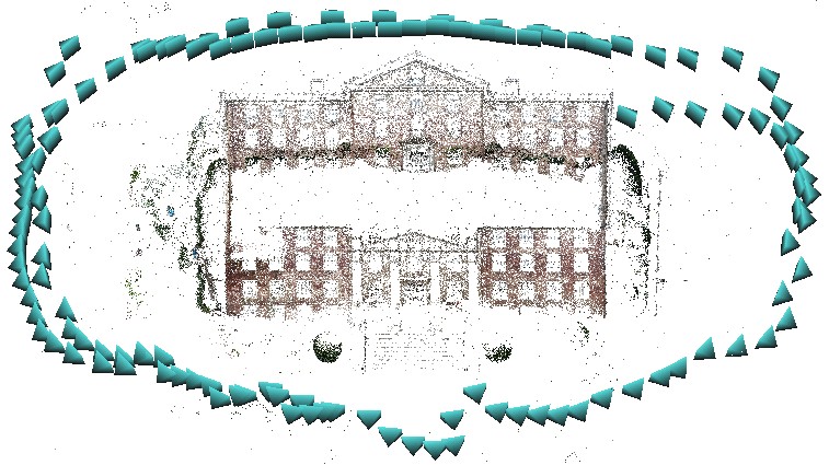
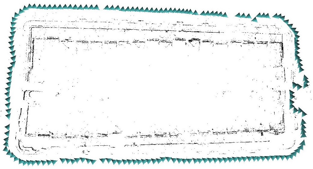
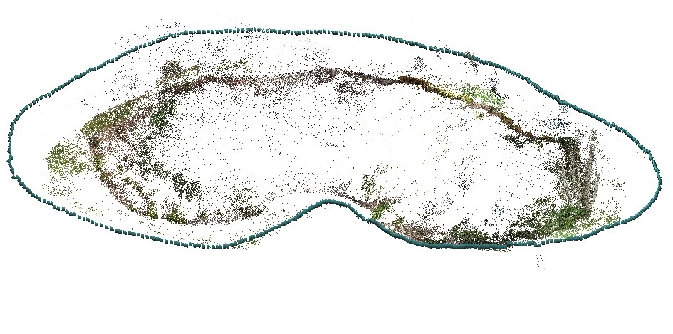
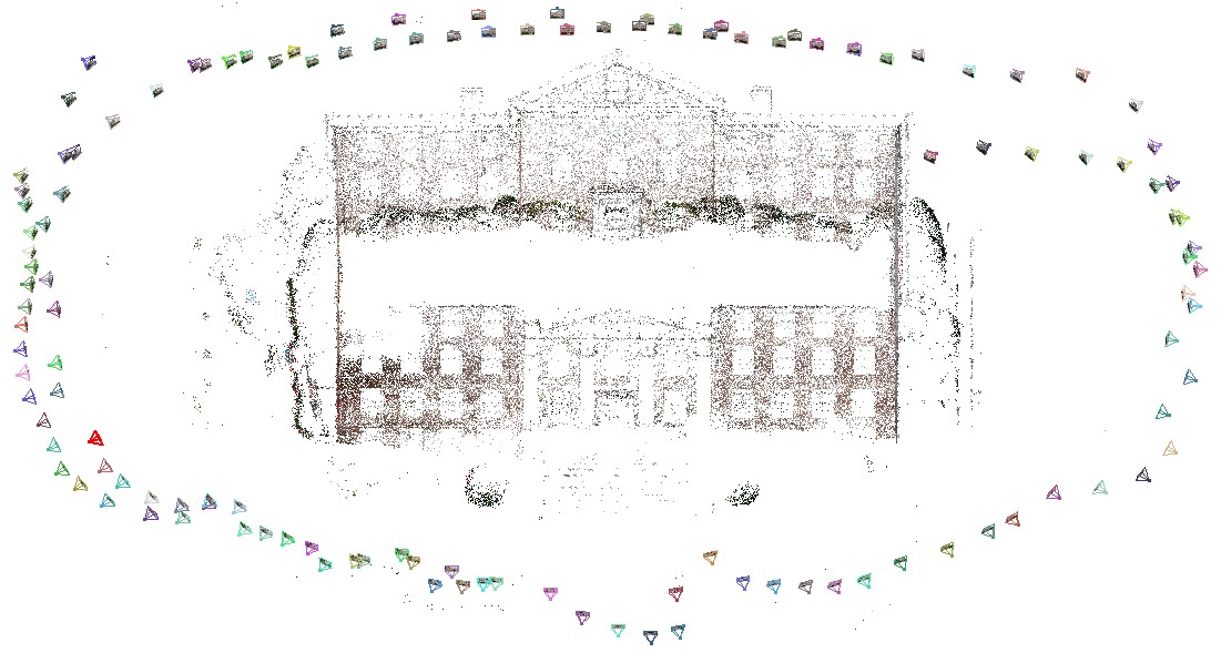
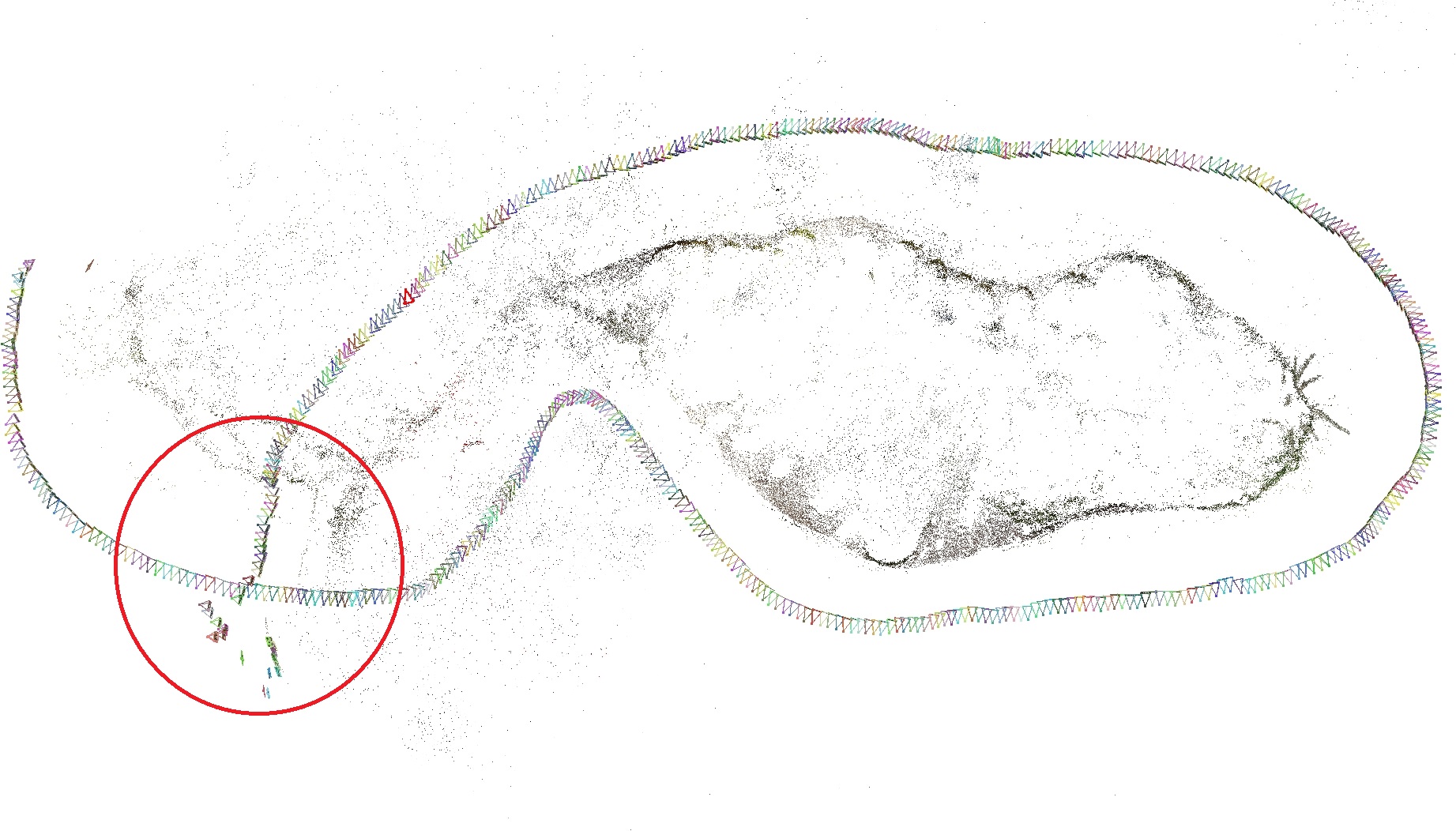
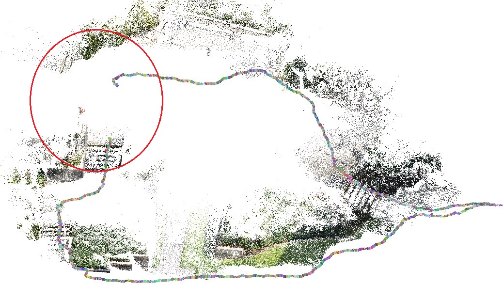
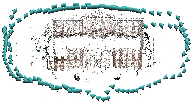
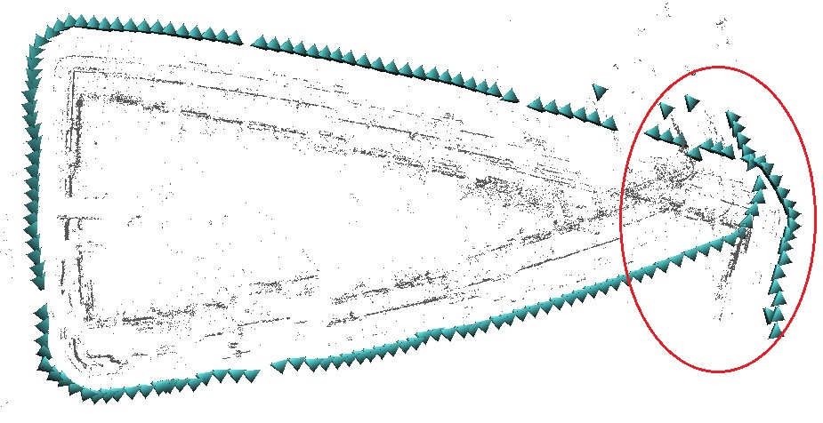
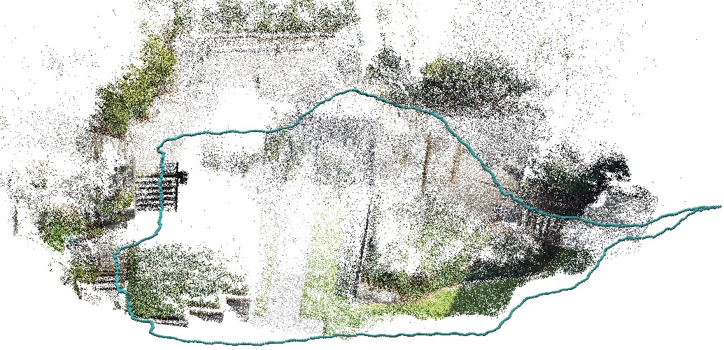
Figure 3 summarizes our experiment on sequentially captured data and compares our method with an incremental method, VisualSFM [Wu(2013)], and some recent global methods [Wilson and Snavely(2014), Özyesil and Singer(2015)]. The test data Building, Street, Park and Stair have 128, 168, 507 and 1221 input images respectively. Generally speaking, VisualSFM [Wu(2013)] suffers from large drifting errors when the input essential matrices are noisy or when the image sequence is long, as shown in the third row of Figure 3. The drifting errors in the Park and Stair examples are severe because of the poor essential matrix estimation due to poor feature localization in their tree images. We do not include results from 1DSfM [Wilson and Snavely(2014)] in Figure 3, since it fails on all these sequential data. Its result on the Street data is shown in Figure 1 (left of top row). 1DSfM cannot handle these examples because it is designed for Internet images which tend to have $O(n^{2})$ essential matrices for $n$ images . The least unsquared deviations (LUD) method [Özyesil and Singer(2015)] generates distortion on the Street example, because it degenerates at collinear motion. In comparison, our method does not have visible drifting and is robust to collinear motion and weak image association.

Dataset		1DSfM[Wilson and Snavely(2014)]				LUD[Özyesil and Singer(2015)]				$L_{2}$		$L_{1}$
Name	$N_{i}$	$N_{c}$	$\tilde{x}$	$\tilde{x}_{BA}$	$\bar{x}_{BA}$	$N_{c}$	$\tilde{x}$	$\tilde{x}_{BA}$	$\bar{x}_{BA}$	$N_{c}$	$\tilde{x}$	$N_{c}$	$\tilde{x}$	$\tilde{x}_{BA}$	$\bar{x}_{BA}$
Alamo	613	529	1.1	0.3	2e7	547	0.4	0.3	2.0	496	0.5	500	0.6	0.5	3.7
Ellis Island	242	214	3.7	0.3	3.0	-	-	-	-	183	9.4	211	3.1	0.6	1.8
Montreal N.D.	467	427	2.5	0.4	1.0	435	0.5	0.4	1.0	424	0.8	426	0.8	0.4	1.1
Notre Dame	552	507	10	1.9	7.0	536	0.3	0.2	0.7	537	0.3	539	0.3	0.2	0.8
NYC Library	369	295	2.5	0.4	1.0	320	2.0	1.4	7.0	-	-	288	1.4	0.9	6.9
Piazza del Popolo	350	308	3.1	2.2	2e2	305	1.5	1.0	4.0	302	3.6	294	2.6	2.4	3.2
Tower of London	499	414	11	1.0	40	425	4.7	3.3	10	311	17	393	4.4	1.1	6.2
Vienna Cathedral	897	770	6.6	0.4	2e4	750	5.4	4.4	10	574	3.6	578	3.5	2.6	4.0
Yorkminster	450	401	3.4	0.1	5e2	404	2.7	1.3	4.0	333	3.9	341	3.7	3.8	14

Table 3: Comparison with [Wilson and Snavely(2014)] on challenging data. $N_{i}$ denotes the number of cameras in the largest connected component of our EG graph, and $N_{c}$ denotes the number of reconstructed cameras. $\tilde{x}$ denotes the median error before BA. $\tilde{x}_{BA}$ and $\bar{x}_{BA}$ denote the median error and the average error after BA respectively. The errors are the distances in meters to corresponding cameras computed by an incremental SfM method [Snavely et al.(2006)Snavely, Seitz, and Szeliski].

Dataset	1DSfM[Wilson and Snavely(2014)]		LUD[Özyesil and Singer(2015)]		Bundler[Snavely et al.(2006)Snavely, Seitz, and Szeliski]	$L_{1}$
	$T_{BA}$	$T_{\Sigma}$	$T_{BA}$	$T_{\Sigma}$	$T_{\Sigma}$	$T_{BA}$	$T_{\Sigma}$
Alamo	752	910	133	750	1654	362	621
Ellis Island	139	171	-	-	1191	64	95
Montreal N.D.	1135	1249	167	553	2710	226	351
Notre Dame	1445	1599	126	1047	6154	793	1159
NYC Library	392	468	54	200	3807	48	90
Piazza del Popolo	191	249	31	162	1287	93	144
Tower of London	606	648	86	228	1900	121	221
Vienna Cathedral	2837	3139	208	1467	10276	717	959
Yorkminster	777	899	148	297	3225	63	108

Table 4: Running times in seconds for the Internet data. $T_{BA}$ and $T_{\Sigma}$ denote the final bundle adjustment time and total running time respectively.

5.3 Experiment on unordered Internet data

The input epipolar geometries for Internet data are quite noisy because of the poor feature matching. Besides using $L_{1}$ optimization, we adopt two additional steps to improve the robustness of our method. After solving camera orientations by the method in [Chatterjee and Govindu(2013)], we further filter input essential matrices with the computed camera orientations. Specifically, for each camera pair, we compare their relative rotation from their global orientation with the relative rotation encoded in their essential matrix. If the difference is larger than a threshold $\varphi_{2}$ (set to $5$ or $10$ degrees), we discard that essential matrix. What’s more, we refine the relative translations with the camera orientations fixed using the method in [Kneip et al.(2011)Kneip, Chli, and Siegwart].

We test our method on the challenging Internet data released by [Wilson and Snavely(2014)] and compare our method with several global methods. We use the results of an optimized incremental SfM system based on Bundler [Snavely et al.(2006)Snavely, Seitz, and Szeliski] as the reference ‘ground-truth’ and compute the camera position errors for evaluation. As shown in Table 3, our method with $L_{1}$ optimization has smaller initial median errors than [Wilson and Snavely(2014)] and comparable errors with [Özyesil and Singer(2015)]. Our method with $L_{1}$ optimization performs better than $L_{2}$ solutions, which shows the effectiveness of the proposed $L_{1}$ method. All the methods have similar results after the final bundle adjustment.

Table 4 lists the running time of different methods. All our experiments were run on a machine with two 2.4GHz Intel Xeon E5645 processors with 16 threads enabled. We cite the running time for [Wilson and Snavely(2014)], [Özyesil and Singer(2015)] and [Snavely et al.(2006)Snavely, Seitz, and Szeliski] for comparison. Our method is around 10 times faster than the optimized incremental method [Snavely et al.(2006)Snavely, Seitz, and Szeliski] and also faster than the global methods [Wilson and Snavely(2014), Özyesil and Singer(2015)].

6 Conclusion

We derive a novel linear method for global camera translation estimation. This method is based on a novel position constraint on cameras linked by a feature track, which minimizes a geometric error and propagates the scale information across far apart camera pairs. In this way, our method works well even on weakly associated images. The final linear formulation does not involve coordinates of scene points, so it is easily scalable and computationally efficient. We further develop an $L_{1}$ optimization method to make the solution robust to outlier essential matrices and feature correspondences. Experiments on various data and comparison with recent works demonstrate the effectiveness of this new algorithm.

Acknowledgements. This work is supported by the NSERC Discovery grant 611664, Discovery Acceleration Supplements 611663, and the HCCS research grant at the ADSC from Singapore’s Agency for Science, Technology and Research (A*STAR).

Appendix

A. Solution for Equation 9.

From Equation 9, we have

$$\vspace{-0.05in}\small\mbox{{\bf e}}_{k+1} = \arg\min_{\mbox{{\bf e}}}\frac{1}{\beta}\left\|\mbox{{\bf e}}\right\|_{1}+\frac{1}{2}\left\|\mbox{{\bf A}}\mbox{{\bf x}}_{k}-\mbox{{\bf e}}+\frac{\lambda_{k}}{\beta}\right\|^{2}$$ (14)

$$= \arg\min_{\mbox{{\bf e}}}\epsilon\left\|\mbox{{\bf e}}\right\|_{1}+\frac{1}{2}\left\|\mbox{{\bf e}}-\mbox{{\bf u}}\right\|^{2},$$

where $\epsilon=\frac{1}{\beta}$, and $\mbox{{\bf u}}=\mbox{{\bf A}}\mbox{{\bf x}}_{k}+\frac{\lambda_{k}}{\beta}$. According to [Lin et al.(2010)Lin, Chen, and Ma], the solution for Equation 14 is

$$\vspace{-0.05in}\small\mbox{{\bf e}}_{k+1}^{i}=\begin{cases}\mbox{{\bf u}}^{i}-\epsilon,&if~{}~{}\mbox{{\bf u}}^{i}>\epsilon,\\ \mbox{{\bf u}}^{i}+\epsilon&if~{}~{}\mbox{{\bf u}}^{i}<-\epsilon,\\ 0,&otherwise,\end{cases}$$ (15)

where $\mbox{{\bf e}}_{k+1}^{i}$ and $\mbox{{\bf u}}^{i}$ are the $i$-th element of e and u.

B. Derivation of Equation 12.

We linearize the quadratic term $\frac{\beta}{2}\left\|\mbox{{\bf A}}\mbox{{\bf x}}-\mbox{{\bf e}}_{k+1}\right\|^{2}$ in Equation 10 at $\mbox{{\bf x}}_{k}$, which gives

$$\vspace{-0.05in}\small\begin{split}\mbox{{\bf x}}_{k+1}&=\arg\min_{\mbox{{\bf x}}\in\Omega}\left\langle\mbox{{\bf A}}^{\top}\lambda_{k},\mbox{{\bf x}}\right\rangle+\left\langle\beta\mbox{{\bf A}}^{\top}(\mbox{{\bf A}}\mbox{{\bf x}}_{k}-\mbox{{\bf e}}_{k+1}),\mbox{{\bf x}}-\mbox{{\bf x}}_{k}\right\rangle+\frac{\beta\eta}{2}\left\|\mbox{{\bf x}}-\mbox{{\bf x}}_{k}\right\|^{2}\\ &=\arg\min_{\mbox{{\bf x}}\in\Omega}\frac{\beta\eta}{2}\left\|\mbox{{\bf x}}-C\right\|^{2},\end{split}$$ (16)

where $\Omega:=\left\{\mbox{{\bf x}}^{\top}\mbox{{\bf x}}=1|\mbox{{\bf x}}\in\mathbb{R}^{n}\right\}$, $C=\mbox{{\bf x}}_{k}-\frac{1}{\eta}\mbox{{\bf A}}^{\top}(\mbox{{\bf A}}\mbox{{\bf x}}_{k}-\mbox{{\bf e}}_{k+1})-\frac{1}{\beta\eta}\mbox{{\bf A}}^{\top}\lambda^{k}$, and $\eta>\sigma_{max}(\mbox{{\bf A}}^{\top}\mbox{{\bf A}})$ is a proximal parameter. Therefore, we can get Equation 12 directly.

References

- [Agarwal et al.()Agarwal, Mierle, and Others] S. Agarwal, K. Mierle, and Others. Ceres solver. http://ceres-solver.org.
- [Agarwal et al.(2008)Agarwal, Snavely, and Seitz] S. Agarwal, N. Snavely, and S. M. Seitz. Fast algorithms for problems in multiview geometry. In Proc. CVPR, pages 1–8, 2008.
- [Agarwal et al.(2009)Agarwal, Snavely, Simon, Seitz, and Szeliski] S. Agarwal, N. Snavely, I. Simon, S. M. Seitz, and R. Szeliski. Building rome in a day. In Proc. ICCV, 2009.
- [Arie-Nachimson et al.(2012)Arie-Nachimson, Kovalsky, Kemelmacher-Shlizerman, Singer, and Basri] M. Arie-Nachimson, S. Z. Kovalsky, I. Kemelmacher-Shlizerman, A. Singer, and R. Basri. Global motion estimation from point matches. In Proc. 3DPVT, 2012.
- [Boyd et al.(2011)Boyd, Parikh, Chu, Peleato, and Eckstein] S. Boyd, N. Parikh, E. Chu, B. Peleato, and J. Eckstein. Distributed optimization and statistical learning via the alternating direction method of multipliers. Found. Trends Mach. Learn., 3(1):1–122, 2011. ISSN 1935-8237.
- [Brand et al.(2004)Brand, Antone, and Teller] M. Brand, M. Antone, and S. Teller. Spectral solution of large-scale extrinsic camera calibration as a graph embedding problem. In Proc. ECCV, 2004.
- [Candes and Tao(2005)] E. J. Candes and T. Tao. Decoding by linear programming. Information Theory, IEEE Transactions on, 51(12):4203–4215, 2005.
- [Chatterjee and Govindu(2013)] A. Chatterjee and V. M. Govindu. Efficient and robust large-scale rotation averaging. In Proc. ICCV, pages 521–528, 2013.
- [Courchay et al.(2010)Courchay, Dalalyan, Keriven, and Sturm] J. Courchay, A. S. Dalalyan, R. Keriven, and P. Sturm. Exploiting loops in the graph of trifocal tensors for calibrating a network of cameras. In Proc. ECCV, pages 85–99, 2010.
- [Crandall et al.(2011)Crandall, Owens, Snavely, and Huttenlocher] D. Crandall, A. Owens, N. Snavely, and D. P. Huttenlocher. Discrete-continuous optimization for large-scale structure from motion. In Proc. CVPR, pages 3001–3008, 2011.
- [Dalalyan and Keriven(2009)] A. Dalalyan and R. Keriven. L1-penalized robust estimation for a class of inverse problems arising in multiview geometry. In NIPS, 2009.
- [Enqvist et al.(2011)Enqvist, Kahl, and Olsson] O. Enqvist, F. Kahl, and C. Olsson. Non-sequential structure from motion. In Workshop on Omnidirectional Vision, Camera Networks and Non-Classical Cameras, 2011.
- [Ferraz et al.(2014)Ferraz, Binefa, and Moreno-Noguer] L. Ferraz, X. Binefa, and F. Moreno-Noguer. Very fast solution to the pnp problem with algebraic outlier rejection. In Proc. CVPR, pages 501–508, 2014.
- [Fitzgibbon and Zisserman(1998)] A. Fitzgibbon and A. Zisserman. Automatic camera recovery for closed or open image sequences. Proc. ECCV, pages 311–326, 1998.
- [Goldstein and Osher(2009)] T. Goldstein and S. Osher. The split bregman method for l1-regularized problems. SIAM Journal on Imaging Sciences, 2(2):323–343, 2009.
- [Govindu(2001)] V. M. Govindu. Combining two-view constraints for motion estimation. In Proc. CVPR, pages 218–225, 2001.
- [Govindu(2004)] V. M. Govindu. Lie-algebraic averaging for globally consistent motion estimation. In Proc. CVPR, 2004.
- [Govindu(2006)] V. M. Govindu. Robustness in motion averaging. In Proc. ACCV, 2006.
- [Haner and Heyden(2012)] S. Haner and A. Heyden. Covariance propagation and next best view planning for 3d reconstruction. In Proc. ECCV, pages 545–556, 2012.
- [Hartley and Zisserman(2003)] R. Hartley and A. Zisserman. Multiple View Geometry in Computer Vision. Cambridge University Press, 2003.
- [Hartley et al.(2013)Hartley, Trumpf, Dai, and Li] R. Hartley, J. Trumpf, Y. Dai, and H. Li. Rotation averaging. IJCV, pages 1–39, 2013.
- [Havlena et al.(2009)Havlena, Torii, Knopp, and Pajdla] M. Havlena, A. Torii, J. Knopp, and T. Pajdla. Randomized structure from motion based on atomic 3d models from camera triplets. In Proc. CVPR, pages 2874–2881, 2009.
- [Jiang et al.(2013)Jiang, Cui, and Tan] N. Jiang, Z. Cui, and P. Tan. A global linear method for camera pose registration. In Proc. ICCV, 2013.
- [Kahl and Hartley(2007)] F. Kahl and R. Hartley. Multiple view geometry under the -norm. IEEE Trans. PAMI, 30:1603–1617, 2007.
- [Kneip et al.(2011)Kneip, Chli, and Siegwart] L. Kneip, M. Chli, and R. Siegwart. Robust real-time visual odometry with a single camera and an imu. In Proc. BMVC, pages 1–11, 2011.
- [Lhuillier and Quan(2005)] M. Lhuillier and L. Quan. A quasi-dense approach to surface reconstruction from uncalibrated images. IEEE Trans. PAMI, 27(3):418–433, 2005.
- [Li(2009)] H. Li. Efficient reduction of l-infinity geometry problems. In Proc. CVPR, pages 2695–2702, 2009.
- [Li and Hartley(2006)] H. Li and R. Hartley. Five-point motion estimation made easy. In Proc. ICPR, pages 630–633, 2006.
- [Lin et al.(2010)Lin, Chen, and Ma] Z. Lin, M. Chen, and Y. Ma. The augmented lagrange multiplier method for exact recovery of corrupted low-rank matrices. arXiv preprint arXiv:1009.5055, 2010.
- [Lin et al.(2011)Lin, Liu, and Su] Z. Lin, R. Liu, and Z. Su. Linearized alternating direction method with adaptive penalty for low-rank representation. In Advances in neural information processing systems, pages 612–620, 2011.
- [Martinec and Pajdla(2007)] D. Martinec and T. Pajdla. Robust rotation and translation estimation in multiview reconstruction. In Proc. CVPR, pages 1–8, 2007.
- [Moulon et al.(2013)Moulon, Monasse, and Marlet] P. Moulon, P. Monasse, and R. Marlet. Global fusion of relative motions for robust, accurate and scalable structure from motion. In Proc. ICCV, 2013.
- [Nistér(2004)] D. Nistér. An efficient solution to the five-point relative pose problem. IEEE Trans. PAMI, 26:756–777, 2004.
- [Olsson et al.(2007)Olsson, Eriksson, and Kahl] C. Olsson, A. Eriksson, and F. Kahl. Efficient optimization for problems using pseudoconvexity. In Proc. ICCV, 2007.
- [Olsson et al.(2010)Olsson, Eriksson, and Hartley] C. Olsson, A. Eriksson, and R. Hartley. Outlier removal using duality. In Proc. CVPR, pages 1450–1457, 2010.
- [Özyesil and Singer(2015)] O. Özyesil and A. Singer. Robust camera location estimation by convex programming. In Proc. CVPR, 2015.
- [Parikh and Boyd(2013)] N. Parikh and S. Boyd. Proximal algorithms. Foundations and Trends in Optimization, 1(3):123–231, 2013.
- [Pollefeys et al.(2004)Pollefeys, Van Gool, Vergauwen, Verbiest, Cornelis, Tops, and Koch] M. Pollefeys, L. Van Gool, M. Vergauwen, F. Verbiest, K. Cornelis, J. Tops, and R. Koch. Visual modeling with a hand-held camera. IJCV, 59:207–232, 2004.
- [Pollefeys et al.(2008)Pollefeys, Nistér, Frahm, Akbarzadeh, Mordohai, Clipp, Engels, Gallup, Kim, Merrell, et al.] M. Pollefeys, D. Nistér, J-M Frahm, A. Akbarzadeh, P. Mordohai, B. Clipp, C. Engels, D. Gallup, S-J Kim, P. Merrell, et al. Detailed real-time urban 3d reconstruction from video. IJCV, 78(2-3):143–167, 2008.
- [Rother(2003)] C. Rother. Multi-View Reconstruction and Camera Recovery using a Real or Virtual Reference Plane. PhD thesis, January 2003.
- [Sim and Hartley(2006)] K. Sim and R. Hartley. Recovering camera motion using minimization. In Proc. CVPR, 2006.
- [Sinha et al.(2010)Sinha, Steedly, and Szeliski] S. Sinha, D. Steedly, and R. Szeliski. A multi-stage linear approach to structure from motion. In ECCV Workshop on Reconstruction and Modeling of Large-Scale 3D Virtual Environments, 2010.
- [Snavely et al.(2006)Snavely, Seitz, and Szeliski] N. Snavely, S. M. Seitz, and R. Szeliski. Photo tourism: exploring photo collections in 3d. ACM Trans. on Graph., 25:835–846, 2006.
- [Snavely et al.(2008)Snavely, Seitz, and Szeliski] N. Snavely, S. M. Seitz, and R. Szeliski. Modeling the world from internet photo collections. IJCV, 80(2):189–210, 2008.
- [Strecha et al.(2008)Strecha, von Hansen, Van Gool, Fua, and Thoennessen] C. Strecha, W. von Hansen, L. Van Gool, P. Fua, and U. Thoennessen. On benchmarking camera calibration and multi-view stereo for high resolution imagery. In Proc. CVPR, 2008.
- [Wilson and Snavely(2014)] K. Wilson and N. Snavely. Robust global translations with 1dsfm. In Proc. ECCV (3), pages 61–75, 2014.
- [Wu(2013)] C. Wu. Towards linear-time incremental structure from motion. In Proc. 3DV, 2013.
- [Zach et al.(2010)Zach, Klopschitz, and Pollefeys] C. Zach, M. Klopschitz, and M. Pollefeys. Disambiguating visual relations using loop constraints. In Proc. CVPR, 2010.